Structure of Random 312-Avoiding Permutations

Abstract

We evaluate the probabilities of various events under the uniform distribution on the set of $312$-avoiding permutations of $1,\ldots,N$. We derive exact formulas for the probability that the $i^{th}$ element of a random permutation is a specific value less than $i$, and for joint probabilities of two such events. In addition, we obtain asymptotic approximations to these probabilities for large $N$ when the elements are not close to the boundaries or to each other. We also evaluate the probability that the graph of a random $312$-avoiding permutation has $k$ specified decreasing points, and we show that for large $N$ the points below the diagonal look like trajectories of a random walk.

1 Introduction

Let $S_{N}$ denote the set of permutations of numbers $1,\ldots,N$ for each positive integer $N$. Given $\tau\in S_{k}$ (with $k\leq N$), we say that a permutation $\sigma=\sigma_{1}\ldots\sigma_{N}$ avoids the pattern $\tau$ (or “$\sigma$ is $\tau$-avoiding”) if there is no subsequence of $\sigma$ with length $k$ having the same relative order as $\tau$. The set of $\tau$-avoiding permutations in $S_{N}$ is denoted by $S_{N}(\tau)$. For example the permutation $435621$ avoids the $312$ pattern and hence $435621\in S_{6}(312)$ but it is not an element of $S_{6}(321)$ since 432, 431, 421, 321, 521, and 621 are subsequences in $435621$ having the $321$ pattern. A permutation $\sigma=\sigma_{1}\ldots\sigma_{N}$ can be represented as a function $\sigma$ that maps $i$ to $\sigma(i)=\sigma_{i}$. The graph of this function is the set of $N$ points $\left\{(i,\sigma_{i}):i=1\ldots N\right\}$ (see Figure 1). Points of the form $(i,\sigma_{i})=(i,i)$ are said to be on the diagonal of the graph of $\sigma$ (these correspond to fixed points of the permutation).

Figure 1: $\sigma=435621\in S_{6}$ viewed as a function $i\mapsto\sigma_{i}$. This is a $312$-avoiding permutation.

The study of pattern-avoiding permutations often reveals connections to other combinatorial objects. For example in [3] it is shown that there is a bijection between $1342$-avoiding permutations and plane forests of $\beta(0,1)$-trees, as well as with ordered collections of rooted bicubic planar maps.

Among other well studied connections of permutations excluding or including certain patterns in the literature are Kazhdan-Lusztig polynomials, singularities of Schubert varieties, Chebyshev polynomials, rook polynomials for Ferrers boards. In a recent book [7] Kitaev goes through a vast amount of literature to point out the connections of permutations with other mathematical objects. Also, Bouvel and Rossin [5] show how permutation patterns are related to problems in computational biology.

One of the initial motivations to study pattern avoiding permutations came from computer science. A basic problem in computer science is sorting $n$ distinct elements in increasing order. Stack sorting is an algorithm that does the sorting operation efficiently, although it only works on some permutations. It was observed that a permutation is stack sortable if and only if it avoids the pattern $231$. A detailed explanation of the connection can be found in Bóna’s book [4]. An important reference on stack sorting is Knuth’s book [8].

Two recent papers of Madras and Liu [11] and Atapour and Madras [1] present numerical and probabilistic approaches to investigate the shapes of random pattern avoiding permutations, mainly of length three, four and five. Both papers include Monte Carlo simulations suggesting the limiting distributions of the positions of points of the permutations. For example Atapour and Madras [1] present the result of Monte Carlo simulation (similar to Figure 2 here) which suggests that typical $312$-avoiding permutations are accumulated near the diagonal as well as below the diagonal. To generate random $312$-avoiding permutations, they run a Markov chain on $S_{N}(312)$ which is irreducible, symmetric and aperiodic [11], and hence has the uniform distribution on $S_{N}(312)$ as its limiting distribution. They further prove the following results that support the findings of the simulations.

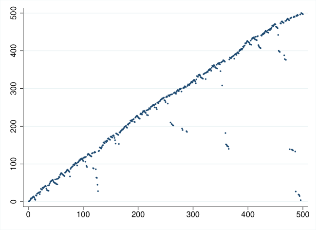
Figure 2: Graph of a randomly generated 312-avoiding permutation with N=500

Definition 1.1.

Consider a pattern $\tau$. For each $N\geq 1$, let $P_{N}^{\tau}$ be the uniform distribution on the set $S_{N}(\tau)$; that is $P_{N}^{\tau}(A)\,=\,\left|A\right|/\left|S_{N}(\tau)\right|$. For simplicity we shall write $P_{N}$ to denote $P_{N}^{312}$ throughout this paper.

Theorem 1.2.

[1] Define the function $K^{*}$ on the unit square $[0,1]^{2}$ by

$$K^{*}(s,t)=\left\{\begin{array}[]{cll}1&\mbox{ if }0\leq t\leq s\leq 1,\\ \frac{1}{4}\frac{(2-s-t)^{2-s-t}(s+t)^{s+t}}{(1-s)^{1-s}(1-t)^{1-t}t^{t}s^{s}}&\mbox{ if }0\leq s\leq t\leq 1.\end{array}\right.$$

Then for any relatively open subset $D$ of $[0,1]^{2}$, we have

$$\lim_{N\rightarrow\infty}\left[P_{N}\left\{\left(\frac{i}{N},\frac{\sigma_{i}}{N}\right)\in D\mbox{ for some }i\in\left\{1,\ldots,N\right\}\right\}\right]^{1/N}=\;\sup\left\{K^{*}(s,t):(s,t)\in D\right\}.$$

Theorem 1.2 concludes that it is rare to have points of the graph well above the diagonal (since $K^{*}(s,t)<1$ for $0<s<t<1$), but it is not rare to have points well below the diagonal. A related result is the following, which says that the number of points well below diagonal is $o(N)$ with high probability.

Proposition 1.3.

[1] Let $\delta>0$, $0<t<1$ and $K_{N}(\sigma,\delta N)=\left|\left\{i:\sigma_{i}<i-\delta N\right\}\right|$. Then

$$\lim_{N\rightarrow\infty}[P_{N}(K_{N}(\sigma,\delta N)>tN)]^{1/N}<1.$$

The present paper is mainly motivated by these results in [1]. In this paper we investigate the probabilities of having a $312$-avoiding permutation that has one or two specified points below the diagonal (i.e., satisfying $\sigma_{i}=j$ for specified $i$ and $j$ with $j<i$). We also extend our results to $k$ decreasing points below the diagonal. Exact evaluations of the probabilities and the approximation results for these probabilities for large $N$ are stated in the next section. Our main theorems imply that the probability of obtaining $312$-avoiding permutations with one specified point below the diagonal is of order $N^{-3/2}$, and the probability of obtaining $312$-avoiding permutations with two (well separated) specified points below the diagonal is of order $N^{-3}$. However, the two-point probability is not approximated by the product of the corresponding one-point probabilities. In particular, Corollary 2.13 describes situations in which two one-point events are positively or negatively correlated. Exact combinatorial results for 312-avoiding permutations with specified points above the diagonal could also be calculated in similar manner; however in this paper we concentrate our attention below the diagonal, as motivated by [1].

While this paper was being written, S. Miner and I. Pak completed a preprint (now [12]) that investigates probabilities of random $123$- and $132$-avoiding permutations with one specified point and their asymptotics. In particular, [12] independently proves Theorems 2.3 and 2.7, and extends these results considerably in directions that we have not pursued.

This paper is organized as follows. Section 2 collects the main results of this paper. Section 3 states the definitions, the basic terminology and results needed for the remaining parts of the paper. Section 4 consists of the proofs of Theorems 2.3, 2.8 and 2.10 which give exact formulas for probabilities of obtaining a $312$-avoiding permutation that has one or two specified points below the diagonal. Theorem 2.3 treats the one point case. Theorem 2.8 considers the case that $\sigma_{i_{1}}=j_{1}>\ldots>\sigma_{i_{k}}=j_{k}$ with $j_{k}<\ldots<j_{1}<i_{1}<\ldots<i_{k}$. Finally, Theorem 2.10 is the case that $\sigma_{i_{1}}=j_{1}<\sigma_{i_{2}}=j_{2}$ with $j_{1}<i_{1}<i_{2}$ and $j_{2}<i_{2}$. Section 5 gives the proofs of Theorems 2.7, 2.9 and 2.11, which are asymptotic approximations of the probabilities calculated in Theorems 2.3, 2.8 and 2.10 respectively. Section 6 proves results related to the limiting distribution of $\sigma$ near the lower right corner of the square $\left[1,N\right]^{2}$, as well as the limiting conditional distribution of $\sigma$ northwest of a given point $(i,j)$ below the diagonal given that $\sigma_{i}=j$.

2 Main Results

Let $C_{N}$ denote the Catalan number, $C_{N}=\frac{1}{N+1}\binom{2N}{N}$ for $N\geq 0$. The proof of the well known result that $\left|S_{N}(\tau)\right|=C_{N}$ for $\tau\in S_{3}$ and $N\geq 1$ can be found in  [4] or  [13].

Definition 2.1.

For $N\in\mathbb{N}$ and $i,j\in[1,N]$, let

$$S^{\bullet}(N,i,j)\;=\;\left\{\sigma\in S_{N}(312):\sigma_{i}=j\right\}\hskip 42.67912pt\hbox{and}$$

$$S^{\Box}(N,i,j)\,=\,\{\sigma\in S_{N}(312):\sigma_{i}=j\hbox{ and }\sigma_{k}<j\hbox{ for all $k\in[1,i)$}\}.$$

Remark 2.2.

Observe that $|S^{\Box}(N,i,j)|=0$ if $j<i$. We also have

$$\left|S^{\Box}(N,i,j)\right|\;=\;\frac{(j-i+1)^{2}}{j(N-i+1)}\binom{2N-i-j}{N-i}\binom{i+j-2}{j-1}\hskip 14.22636pt\mbox{whenever }1\leq i\leq j\leq N.$$

For $i<j$, this was proven in [1]. For the case $i=j$, we note that for every $\sigma\in S^{\Box}(N,j,j)$, we have $\sigma_{k}>j$ for every $k>j$. Therefore $\left|S^{\Box}(N,j,j)\right|=|S_{j-1}(312)|\times|S_{N-j}(312)|\,\,=C_{j-1}C_{N-j}\,=\,\frac{1}{j(N-j+1)}\binom{2N-2j}{N-j}\binom{2j-2}{j-1}$.

Our first result gives the cardinality of $S^{\bullet}(N,N-t,j)$.

Theorem 2.3.

Let $j<N-t$. Then

$$\left|S^{\bullet}(N,N-t,j)\right|=\sum_{i_{0}=\max\left\{1,j-t\right\}}^{j}C_{N-t-i_{0}}\frac{(j-i_{0}+1)^{2}}{j(t+1)}\binom{i_{0}+2t-j}{t}\binom{i_{0}+j-2}{j-1}.$$

We shall prove Theorem 2.3 by constructing a natural bijection between $S^{\bullet}(N,N-t,j)$ and

$\bigcup_{i_{0}=\max\left\{1,j-t\right\}}^{j}S_{N-t-i_{0}}(312)\times S^{\Box}(t+i_{0},i_{0},j)$ for fixed $N,t$ and $j$ (see Definition 4.5). We shall use this bijection repeatedly for the proof of Theorem 2.8, and a closely related bijection for the proof of Theorem 2.10.

Remark 2.4.

It is not hard to check that $\left|S^{\bullet}(N,N-t,j)\right|=\left|S^{\bullet}(N,N-j,t)\right|.$

Remark 2.5.

Theorem 2.3 also gives the probability $P_{N}(S^{\bullet}(N,i,j))$, since by definition it is equal to $\frac{\left|S^{\bullet}(N,N-t,j)\right|}{|S_{N}(312)|}$. This applies to Theorems 2.8 and 2.10 as well.

Notation 2.6.

In preparation for upcoming results, we state our conventions on asymptotics. We write $f(N)\sim g(N)$ to mean that $\lim_{N\rightarrow\infty}f(N)/g(N)=1$. We write $f(N)\asymp g(N)$ to mean that there exists a constant $C>0$ such that $C>g(N)/f(N)>C^{-1}$ for all sufficiently large $N$. We write $f(N)\prec\!\prec g(N)$ to mean that there is an $\epsilon>0$ such that $g(N)-f(N)>\epsilon N$ for all sufficiently large $N$.

For example, the statement “$f(i,j,N)\,=\,O(N)$ for $i\prec\!\prec j$” would mean that for any $\epsilon>0$, there exists a $C$ and $N_{1}$ such that $\left|f(i,j,N)\right|\leq CN$ for all $i$, $j$, and $N$ such that $j-i>\epsilon N$ and $N\geq N_{1}$ (where $C$ and $N_{1}$ can depend on $\epsilon$).

Theorem 2.7.

Fix $0<\theta<\frac{1}{6}$. Then

$$P_{N}(S^{\bullet}(N,N-t,j))=\frac{N^{-3/2}}{2\sqrt{\pi}\left(1-\frac{N-t-j}{N}\right)^{3/2}\left(\frac{N-t-j}{N}\right)^{3/2}}(1+O(N^{3\theta-\frac{1}{2}}))$$

for $0\prec\!\prec j\prec\!\prec i\prec\!\prec N$.

Figure 3: These diagrams represents the requirement that a permutation has specified points $\sigma_{N-t_{1}}=j_{1}$ and $\sigma_{N-t_{2}}=j_{2}$ where $j_{1}<N-t_{1}$, $j_{2}<N-t_{2}$, and $N-t_{1}<N-t_{2}$. The left diagram corresponds to Theorem 2.8 for $k=2$ and the right one corresponds to Theorem 2.10.

Theorem 2.8.

Let $j_{k}<j_{k-1}<\ldots<j_{1}<N-t_{1}<\ldots<N-t_{k}$ and define

$$S^{{\searrow}_{k}}(N)\;\equiv\;S^{{\searrow}_{k}}(N,N-t_{1},\ldots,N-t_{k},j_{1},\ldots,j_{k})=\left\{\sigma\in S_{N}(312):\sigma_{N-t_{1}}=j_{1},\,\ldots\,\sigma_{N-t_{k}}=j_{k}\right\}.$$

Then,

$$\left|S^{\searrow_{k}}(N)\right|\;=\sum_{i=\max\left\{1,j_{k}-t_{k}\right\}}^{j_{k}}\frac{(j_{k}-i+1)^{2}}{j_{k}(t_{k}+1)}\binom{i+2t_{k}-j_{k}}{t_{k}}\binom{i+j_{k}-2}{j_{k}-1}\times$$

$$\left|S^{\searrow_{k-1}}(N-t_{k}-i,N-t_{1}-i+1\ldots,N-t_{k-1}-i+1,j_{1}-j_{k},j_{2}-j_{k},\ldots,j_{k-1}-j_{k})\right|.$$

In particular for $k=2$ we have

$$\left|S^{\searrow_{2}}(N)\right|\equiv\left|S^{\searrow}(N)\right|\;= \sum_{i_{1}=\max\left\{1,j_{2}-t_{2}\right\}}^{j_{2}}\frac{(j_{2}-i_{1}+1)^{2}}{j_{2}(t_{2}+1)}\binom{i_{1}+2t_{2}-j_{2}}{t_{2}}\binom{i_{1}+j_{2}-2}{j_{2}-1}\times$$

$$\sum_{i_{0}=\max\left\{1,(j_{1}-j_{2})-(t_{1}-t_{2}-1)\right\}}^{j_{1}-j_{2}}C_{N-t_{1}-i_{1}-i_{0}+1}\frac{(j_{1}-j_{2}-i_{0}+1)^{2}}{(j_{1}-j_{2})(t_{1}-t_{2})}\times$$

$$\binom{i_{0}+2(t_{1}-t_{2}-1)-(j_{1}-j_{2})}{t_{1}-t_{2}-1}\binom{i_{0}+j_{1}-j_{2}-2}{j_{1}-j_{2}-1}.$$

Theorem 2.9.

Fix $0<\theta<\frac{1}{6}$. Then

$$P_{N}\left(S^{\searrow}(N)\right)=\frac{1}{4\pi}\frac{N^{-3}}{\left(\frac{(N-t_{2}-j_{2})-(N-t_{1}-j_{1})}{N}\right)^{3/2}\left(\frac{N-t_{1}-j_{1}}{N}\right)^{3/2}\left(1-\frac{N-t_{2}-j_{2}}{N}\right)^{3/2}}(1+O(N^{3\theta-1/2}))$$

for $0\prec\!\prec j_{2}\prec\!\prec j_{1}\prec\!\prec N-t_{1}\prec\!\prec N-t_{2}\prec\!\prec N$.

Theorem 2.10.

For $N,j_{1},j_{2},t_{1},t_{2}\in\mathbb{N}$ such that $j_{1}<N-t_{1}<N-t_{2}$, $j_{1}<j_{2}<N-t_{2}$, define $S^{\nearrow}(N)\equiv S^{\nearrow}(N,N-t_{1},N-t_{2},j_{1},j_{2})=\left\{\sigma\in S_{N}(312):\sigma_{N-t_{1}}=j_{1},\sigma_{N-t_{2}}=j_{2}\right\}$.

(a) If $j_{2}<N-t_{1}+1$, then $\left|S^{\nearrow}(N)\right|=0$.

(b) If $j_{2}\geq N-t_{1}+1$, then

$$\left|S^{\nearrow}(N)\right|\; =\sum_{i_{1}=\max\left\{1,j_{1}-j_{2}+N-t_{1}+1\right\}}^{j_{1}}\sum_{i_{2}=\max\left\{N-t_{1}+1,j_{2}-t_{2}\right\}}^{j_{2}}C_{N-t_{1}-i_{1}}C_{N-t_{2}-i_{2}}\times$$

$$\frac{(j_{1}-i_{1}+1)(j_{2}-i_{2}+1)}{j_{1}(t_{2}+1)}\binom{j_{1}+i_{1}-2}{j_{1}-1}\binom{i_{2}+2t_{2}-j_{2}}{t_{2}}\times$$

$$\left(\binom{i_{1}+i_{2}+j_{2}-j_{1}-2(N-t_{1}+1)}{j_{2}+(i_{1}-j_{1}-1)-(N-t_{1})}-\binom{i_{1}+i_{2}+j_{2}-j_{1}-2(N-t_{1}+1)}{j_{2}-(N-t_{1})}\right).$$

Theorem 2.11.

Fix $0<\theta<\frac{1}{6}$. Then,

$$P_{N}(S^{\nearrow}(N))=$$

$$\frac{N^{-3}}{4\pi\left(1-\frac{(N-t_{1}-j_{1})+(N-t_{2}-j_{2})}{N}\right)^{3/2}\left(\frac{N-t_{1}-j_{1}}{N}\right)^{3/2}\left(\frac{N-t_{2}-j_{2}}{N}\right)^{3/2}}(1+O(N^{3\theta-\frac{1}{2}}))$$

for $0\prec\!\prec j_{1}\prec\!\prec N-t_{1}\prec\!\prec j_{2}\prec\!\prec N-t_{2}\prec\!\prec N$.

The next corollary restates Theorem 2.7 for the special case that $j=\left\lfloor\alpha N\right\rfloor$, $i=N-t=\left\lfloor\beta N\right\rfloor$. Corollary 2.13 contains the analogous statements for Theorems 2.9 and 2.11. Corollary 2.13 also frames these results in terms of a random field corresponding to points in the graph of a random $\sigma$.

Corollary 2.12.

Assume that $0<\alpha<\beta<1$. Then

$$P_{N}(S^{\bullet}(N,\left\lfloor\beta N\right\rfloor,\left\lfloor\alpha N\right\rfloor))\;\sim\;\frac{N^{-3/2}}{2\sqrt{\pi}(1-(\beta-\alpha))^{3/2}(\beta-\alpha)^{3/2}}.$$

Corollary 2.13.

Let $i_{1}=\left\lfloor\beta_{1}N\right\rfloor,i_{2}=\left\lfloor\beta_{2}N\right\rfloor,j_{1}=\left\lfloor\alpha_{1}N\right\rfloor,j_{2}=\left\lfloor\alpha_{2}N\right\rfloor$. Also let $\Delta_{1}=\beta_{1}-\alpha_{1}$ and $\Delta_{2}=\beta_{2}-\alpha_{2}$. For a random $\sigma$ having distribution $P_{N}$, let $Z(i,j)$ be the indicator of the event that $\sigma_{i}=j$, and let Cov_N denote covariance with respect to $P_{N}$.
(a) Assume that $0<\alpha_{2}<\alpha_{1}<\beta_{1}<\beta_{2}<1$. Then

$$P_{N}\left(S^{\searrow}(N)\right)\;\sim\;\frac{1}{4\pi}\frac{N^{-3}}{[(\Delta_{2}-\Delta_{1})\Delta_{1}(1-\Delta_{2})]^{3/2}}\hskip 22.76219pt\hbox{and}$$

$$\lim_{N\rightarrow\infty} N^{3}\,\textrm{\em Cov}_{N}(Z(i_{1},j_{1}),Z(i_{2},j_{2}))\;=\;\frac{\left(\left[\frac{\Delta_{2}(1-\Delta_{1})}{\Delta_{2}-\Delta_{1}}\right]^{3/2}-1\right)}{4\pi\,[\Delta_{1}\Delta_{2}(1-\Delta_{1})(1-\Delta_{2})]^{3/2}}\;>\;0\,.$$

(b) Assume that $0<\alpha_{1}<\beta_{1}<\alpha_{2}<\beta_{2}<1$. Then

$$P_{N}\left(S^{\nearrow}(N)\right)\;\sim\;\frac{1}{4\pi}\frac{N^{-3}}{[(1-\Delta_{1}-\Delta_{2})\Delta_{1}\Delta_{2}]^{3/2}}\hskip 22.76219pt\hbox{and}$$

$$\lim_{N\rightarrow\infty} N^{3}\,\textrm{\em Cov}_{N}(Z(i_{1},j_{1}),Z(i_{2},j_{2}))\;=\;\frac{\left(\left[\frac{(1-\Delta_{1})(1-\Delta_{2})}{1-\Delta_{1}-\Delta_{2}}\right]^{3/2}-1\right)}{4\pi\,[\Delta_{1}\Delta_{2}(1-\Delta_{1})(1-\Delta_{2})]^{3/2}}\;>\;0\,.$$

(c) Assume that $0<\alpha_{1}<\alpha_{2}<\beta_{1}<\beta_{2}<1$. Then $P_{N}\left(S^{\nearrow}(N)\right)\,=\,0$ and

$$\lim_{N\rightarrow\infty}N^{3}\,\textrm{\em Cov}_{N}(Z(i_{1},j_{1}),Z(i_{2},j_{2}))\;=\;\frac{-1}{4\pi\,[\Delta_{1}\Delta_{2}(1-\Delta_{1})(1-\Delta_{2})]^{3/2}}\;<\;0\,.$$ (1)

The above asymptotic results hold for points well below the diagonal and well away from the sides of the square $[1,N]^{2}$.

The next results concern the lower right corner of the square. Our starting point is Proposition 2.15, of which part (a) has also been observed by Miner and Pak [12].

Definition 2.14.

For all $a,b\in\mathbb{N}$ define

$$\rho(a,b)\;=\;\sum_{i_{0}=\max\left\{1,b-a+1\right\}}^{b}\frac{(b-i_{0}+1)^{2}}{ba4^{i_{0}+a-1}}\binom{i_{0}+2(a-1)-b}{a-1}\binom{i_{0}+b-2}{b-1}.$$

We note that we can also write $\rho(a,b)\,=\,\sum_{i=\max\left\{1,b-a+1\right\}}^{b}|S^{\Box}(i+a-1,i,b)|/4^{i+a-1}$ (recall Definition 2.1 and Remark 2.2).

Proposition 2.15.

(a) Fix $a,b\in\mathbb{N}$. Then

$$\lim_{N\rightarrow\infty}P_{N}(S^{\bullet}(N,N{-}a{+}1,b))\;=\;\rho(a,b).$$

(b) More generally, let $k\in\mathbb{N}$ and let $a_{1},\ldots,a_{k},b_{1},\ldots b_{k}\in\mathbb{N}$. Define $A_{m}=\sum_{l=1}^{m}a_{l}$, $B_{m}=\sum_{l=1}^{m}b_{l}$ for $m=1,\ldots,k$. Then

$$P_{N}(S^{\searrow k}(N,N{-}A_{k}{+}1,\ldots,N{-}A_{1}{+}1,B_{k},\ldots,B_{1}))\;=\;\left[\prod_{v=1}^{k}\rho(a_{v},b_{v})\right](1+O(N^{-1})).$$

By Remark 2.4, we also observe that $\rho$ is symmetric in $a$ and $b$.

Our next task is to expand part (b) above into a more complete limiting description of $\sigma$ near the lower right corner of the square $[1,N]^{2}$. Since we consider $N\rightarrow\infty$, we shall translate the lower right corner so that the square expands to fill the second quadrant.

Definition 2.16.

Let $Q:=\{(-i,j):i,j\in\mathbb{N}\}$ be the integer points inside the second quadrant. For $N\in\mathbb{N}$, let $W_{N}:=[-N,-1]\times[1,N]$ be the $N\times N$ square in the lower right corner of $Q$. For each $N$, define the collection of (dependent) binary random variables $\{X^{N}_{(-i,j)}:(-i,j)\in Q\}$ by

$$X^{N}_{(-i,j)}\;=\;\begin{cases}1&\mbox{if $(-i,j)\in W_{N}$ and $\sigma_{N-i+1}=j$ }\\ 0&\mbox{otherwise}\end{cases}$$

where $\sigma$ has the distribution $P_{N}$. We will often write “$q$” (or sometimes “$r$” or “$s$”) to represent a generic element $(-i,j)$ of $Q$; e.g. we can refer to the above collection as $\{X^{N}_{q}:q\in Q\}$.

Figure 4: The solid circles show three points of the graph of a permutation in $S^{{\searrow}3}(N,N{-}4,N{-}6,2,4,7)$. Such a permutation gives the values $X^{N}_{(-1,2)}=1=X^{N}_{(-5,4)}=X^{N}_{(-7,7)}$ (and hence $X^{N}_{(-7,j)}=0$ for all $j\neq 7$, etc.).

See Figure 4. Note that the random set $\{q\in Q:X^{N}_{q}=1\}$ is essentially the graph of the random permutation $\sigma$.

With the above definition, Proposition 2.15(b) concludes that the probability that $X^{N}_{(-A_{m},B_{m})}=1$ for every $m=1,\ldots,k$ converges to $\rho(a_{1},\ldots,b_{k})$ as $N\rightarrow\infty$. Our next result builds on this to show that there is a limiting collection of random variables indexed by points of $Q$.

Theorem 2.17.

There exists a collection of $\{0,1\}$-valued random variables $\{X_{q}:q\in Q\}$ (with joint distribution $P_{\infty}$) such that for every finite subset $C$ of $Q$, the collection $\{X^{N}_{q}:q\in C\}$ converges in distribution to $\{X_{q}:q\in C\}$ as $N\rightarrow\infty$.

The product form of the limit in Proposition 2.15(b) implies that the limiting collection of random variables $\{X_{q}:q\in Q\}$ has a kind of two-dimensional regenerative property, analogous to the more standard regenerative property on $\mathbb{N}$ possessed by discrete renewal processes (see [6]). Our two-dimensional renewal structure is fully described in Theorem 2.19, using the following notation.

Definition 2.18.

For $a,b\in\mathbb{N}$, let

$$\pi(-a,b)\;=\;\frac{C_{a-1}C_{b-1}}{4^{a+b-1}}.$$

It is not hard to see that $\pi$ is a probability distribution on $Q$. (Indeed, using the well-known Catalan generating function $G(z)\,=\,\sum_{i=0}^{\infty}C_{i}z^{i}\,=\,(1-\sqrt{1-4z})/2z$ (e.g. [4]), we have $\sum_{a,b=1}^{\infty}\pi(-a,b)\,=\,\frac{1}{4}\,G\left(\frac{1}{4}\right)^{2}\,=\,1$.) This distribution plays a key role in the following theorem.

Theorem 2.19.

The set $W^{*}=\{q\in Q:X_{q}=1\}$ is an infinite random set of the form $\{\vec{V}_{m}:m\in\mathbb{N}\}$ where $\{(\vec{V}_{m}-\vec{V}_{m-1}):m\in\mathbb{N}\}$ are i.i.d. $Q$-valued random vectors with distribution $\pi(-a,b)$ [writing $\vec{V}_{0}=(0,0)$]. Moreover, the components of $\vec{V}_{1}$ have infinite means.

In particular, Theorem 2.19 tells us that, with probability one, the random set $W^{*}=\{q\in Q:X_{q}=1\}$ is an infinite sequence of points $\left\{(-A_{m},B_{m})\right\}$ such that the sequences $\{A_{m}\}$ and $\{B_{m}\}$ are both strictly increasing. Moreover, the distribution of $W^{*}$ is exactly that of the set of points visited by a random walk with jump distribution $\pi$. Observe that such a random walk only jumps to the north and west. (Here, “random walk” denotes a process which is the sequence of partial sums of an i.i.d. sequence of vectors.)

To illustrate our results, note that Proposition 2.15(b) tells us that the probability of observing the three points shown in Figure 4 is approximately $\rho(1,2)\rho(4,2)\rho(2,3)$ for large $N$. In contrast, Theorem 2.19 says that the probability of observing these three points and having no other points in $[N{-}6,N]\times[1,7]$ is approximately $\pi(-1,2)\pi(-4,2)\pi(-2,3)$.

Our final theorem says that if we condition on the event $\{\sigma_{N-t+1}=j\}$ (i.e. $\{X^{N}_{(-t,j)}=1\}$) and let $N$ get large while $(N-t,j)$ remains well below the diagonal, then the conditional distribution of points above and to the left of $(N-t,j)$ (and near $(N-t,j)$) approaches the (unconditional) distribution of points in the lower right corner of the square $[1,N]^{2}$.

Theorem 2.20.

Let $D$ and $F$ be disjoint finite subsets of $Q$. Then

$$\lim_{N-t-j\rightarrow\infty} P_{N}(X^{N}_{q+(-t,j)}=1\;\;\forall q\in D\mbox{ and }X^{N}_{r+(-t,j)}=0\;\;\forall r\in F\,|\,X^{N}_{(-t,j)}=1)$$

$$= \;P_{\infty}(X_{q}=1\;\;\forall q\in D\mbox{ and }X_{r}=0\;\;\forall r\in F)\,.$$

3 Terminology and Useful Results

3.1 Pattern Avoiding Permutations and Dyck Paths

Although we focus on the pattern 312, we first give a general definition of pattern avoidance.

Definition 3.1.

Let $k$ be a positive integer $k\geq 2$ and $\tau=\tau_{1}\ldots\tau_{k}\in S_{k}.$

• We say that a string of $k$ distinct integers $\alpha_{1}\ldots\alpha_{k}$ forms the pattern $\tau$ if for each $i=1,\ldots,k$, $\alpha_{i}$ is the $\tau_{i}$th smallest element of $\{\alpha_{1},\ldots,\alpha_{k}\}$. In this case we also write $\tau\,=\,\mathbf{Patt}(\alpha_{1},\ldots,\alpha_{k})$.

• We say that $\sigma\in S_{N}$ contains pattern $\tau$ if some $k$-element subsequence $\sigma_{i_{1}}\sigma_{i_{2}}\ldots\sigma_{i_{k}}$ of $\sigma$ occurs with the same relative order as $\tau=\tau_{1}\ldots\tau_{k}$, i.e. $\tau=\mathbf{Patt}(\sigma_{i_{1}},\ldots,\sigma_{i_{k}})$. If $\sigma$ does not contain the pattern $\tau$, then we say $\sigma$ avoids $\tau$. Let $S_{N}(\tau)$ be the set of permutations of $\left\{1,\ldots N\right\}$ that avoid $\tau$.

Explicitly, a permutation $\sigma$ avoids the pattern $312$ if $\sigma$ has no subsequence of three elements that has same relative order as $312$, i.e., if there does not exist $i_{1}<i_{2}<i_{3}$ such that $\sigma_{i_{1}}>\sigma_{i_{3}}>\sigma_{i_{2}}$. See Figure 1 for an example.

Definition 3.2.

A Dyck segment from $(X_{0},Y_{0})$ to $(X_{K},Y_{K})$ is a sequence $(X_{0},Y_{0}),(X_{1},Y_{1}),\ldots,$ $(X_{K},Y_{K})$ in $\mathbb{Z}^{2}$ such that and $X_{0}$ and $Y_{0}$ are nonnegative integers and

$$X_{i}-X_{i-1}=1\text{, }\;Y_{i}-Y_{i-1}\in\left\{-1,+1\right\}\text{, and }\;Y_{i}\geq 0\text{\hskip 8.53581ptfor every $i=1,\ldots,K$.}$$ (2)

A Dyck path of length $2L$ is a Dyck segment from $(0,0)$ to $(2L,0)$. See Figure 6 below for an example.

Lemma 3.3.

[14] The set $D$ of all Dyck segments from $(X_{0},Y_{0})$ to $(X_{K},Y_{K})$ has $\left|D\right|=0$ iff at least one of the following conditions holds:

(a) $X_{0}\,>\,X_{K}$,

(b) $|Y_{K}-Y_{0}|\,>\,X_{K}-X_{0}$,

(c) $Y_{K}-Y_{0}\neq X_{K}-X_{0}\,(mod\,2)$ (i.e., one of $Y_{K}-Y_{0}$ or $X_{K}-X_{0}$ is even and the other is odd).

Otherwise,

$$\left|D\right|\;=\;\binom{X_{K}-X_{0}}{\frac{X_{K}-X_{0}+\left|Y_{K}-Y_{0}\right|}{2}}-\binom{X_{K}-X_{0}}{\frac{X_{K}-X_{0}+Y_{K}+Y_{0}+2}{2}}\;=\;\binom{X_{K}-X_{0}}{\frac{X_{K}-X_{0}+Y_{K}-Y_{0}}{2}}-\binom{X_{K}-X_{0}}{\frac{X_{K}-X_{0}+Y_{K}+Y_{0}+2}{2}}.$$

Remark 3.4.

For Dyck segments from $(0,0)$ to $(X_{K},Y_{K})$, the result of Lemma 3.3 can be rewritten as

$$\left|D\right|\;=\;\frac{2Y_{k}+2}{X_{k}+Y_{k}+2}\binom{X_{k}}{\frac{X_{k}+Y_{k}}{2}}.$$

Definition 3.5.

$(X_{i},Y_{i})$ is a peak of a given Dyck path if $Y_{i-1}=Y_{i+1}=Y_{i}-1$.

Krattenthaler [9] proves that there is a bijection between $S_{N}(132)$ and the set $D_{N}$ of all Dyck paths of length $2N$. We restate his result by replacing $132$-avoiding permutations by its complement $312$-avoiding permutations. A different bijective proof between Dyck paths and $S_{N}(312)$ can also be found in [2].

Let $\pi\in S_{N}(312)$ and $\pi=\pi_{1}\pi_{2}\ldots\pi_{N}$. Following the steps of Krattenthaler’s proof we first determine the left-to-right maxima in $\pi$. A left-to-right maximum is an element $\pi_{i}$ which is greater than all the elements to its left, i.e., larger than all $\pi_{j}$ with $j<i$. For example left-to-right maxima in the permutation $25647318$ are $2,5,6,7$ and $8$. Let the left-to-right maxima in $\pi$ be $M_{1},M_{2},\dots,M_{s}$ so that $\pi=M_{1}W_{1}M_{2}W_{2}\ldots M_{s}W_{s}$ where $W_{i}$ is the (possibly empty) subword of $\pi$ in between $M_{i}$ and $M_{i+1}$. Then any left-to-right maximum is translated into $M_{i}-M_{i-1}$ up-steps (with the convention that $M_{0}=0$). Any subword $W_{i}$ is translated into $\left|W_{i}\right|+1$ down-steps (where $\left|W_{i}\right|$ denotes the number of elements of $W_{i}$). Hence, if $\pi_{i}=M_{t}$ for some $t\leq i$, then the corresponding point on the Dyck path has its horizontal component equal to $\sum_{k=1}^{t}(M_{k}-M_{k-1})+\sum_{k=1}^{t-1}\left|W_{k}\right|+(t-1)$. Observe that $\sum_{k=1}^{t-1}\left|W_{k}\right|$ counts the number of elements that are not a maximum up until the $t$-th maximum $M_{t}$, and $t-1$ counts the previous maxima $M_{1},\ldots,M_{t-1}$. Together they count the number of all positions to the left of $i$, which is $i-1$, i.e., $\sum_{k=1}^{t-1}\left|W_{k}\right|+(t-1)=i-1$. Hence, the horizontal component of the point on the Dyck path corresponding to $\pi_{i}=M_{t}$ is $M_{t}+(i-1)$. Similarly, the vertical component of the point on the Dyck path corresponding to $\pi_{i}=M_{t}$ is $M_{t}-(i-1)$. Therefore, the left-to-right maximum $M_{t}$ at position $i$ corresponds to a peak $(M_{t}+(i-1),M_{t}-(i-1))$ in the corresponding Dyck path. For example, Figures 6 and 6 show the correspondence between the permutation $\pi=25647318$ and its Dyck path. The fourth left-to-right maximum in Figure 6, namely 7 (circled), corresponds to the peak $(11,3)$ in Figure 6 (dashed lines). Observe that a clockwise $45^{\circ}$ rotation of the dashed lines in Figure 6 produces the diagonal lines and horizontal axis of Figure 6. Explicitly, this rotation maps a point $(x,y)$ in Figure 6 to the point $(x+y-1,y-x+1)$ in Figure 6.

Figure 5: $\pi=25647318$ with diagonal segment corresponding to x-axis in Figure 6. Here, $M_{1}=2$, $M_{4}=7$, $W_{1}$ is empty, and $W_{4}=31$.

Figure 6: Dyck path of length 16 corresponding to $\pi=25647318$.

3.2 Approximations of Integrals

We first record two results that will be useful in Section 5 for obtaining the asymptotic behaviors of sums. For a function $g$, let $\|g\|_{\infty}$ be the supremum of $|g|$ over its domain.

Proposition 3.6.

Let $f:[0,\infty)\rightarrow\mathbb{R}$ be continuous and differentiable. Let $\Delta>0$, $R\in\mathbb{N}$, and define $X_{i}=i\Delta$ for $i=1,2,\ldots,R$. Also let $J=\sum_{i=1}^{R}f(X_{i})\Delta$ and $I=\int_{0}^{R\Delta}f(x)\,dx$. Then

$$\left|J-I\right|\;\leq\;\|f^{{}^{\prime}}\|_{\infty}\frac{\Delta^{2}R}{2}.$$

Proposition 3.7.

Let $\tilde{f}:[0,\infty)^{2}\rightarrow\mathbb{R}$ be continuous and differentiable. Let $\Delta>0$, $R\in\mathbb{N}$, and $Y_{i}=X_{i}=i\Delta$ for $i=1,2,\ldots,R$. Let $\tilde{J}=\sum_{i=1}^{R}\sum_{j=1}^{R}\tilde{f}(X_{i},Y_{j})\Delta^{2}$, $\tilde{I}=\int_{0}^{R\Delta}\int_{0}^{R\Delta}\tilde{f}(x,y)\,dx\,dy$, and $C_{\tilde{f}}:=\max\left\{\left\|\frac{\partial\tilde{f}}{\partial x}\right\|_{\infty},\left\|\frac{\partial\tilde{f}}{\partial y}\right\|_{\infty}\right\}$. Then

$$\left|\tilde{J}-\tilde{I}\right|\;\leq\;C_{\tilde{f}}\Delta^{3}R^{2}.$$

In particular, suppose $\theta>0$, $R=R_{N}=\left\lceil N^{1/2+\theta}\right\rceil$, and $\Delta=\Delta_{N}=N^{-1/2}$. Then in Proposition 3.6, the sums $I=I(N)$ and $J=J(N)$ satisfy

$$\left|J(N)-I(N)\right|\;=\;O(N^{\theta-1/2}),$$

and in Proposition 3.7 the sums $\tilde{I}=\tilde{I}(N)$ and $\tilde{J}=\tilde{J}(N)$ satisfy

$$\left|\tilde{J}(N)-\tilde{I}(N)\right|\;=\;O(N^{2\theta-1/2}).$$

Such results are well known. For example, Proposition 3.7 holds because

$$\left|\int^{b}_{b-\Delta}\int^{a}_{a-\Delta}(\tilde{f}(x,y)-\tilde{f}(a,b))\,dx\,dy\right|\;\leq\;\int^{b}_{b-\Delta}\int^{a}_{a-\Delta}(|a-x|+|b-y|)\,C_{\tilde{f}}\,dx\,dy\;=\;\Delta^{3}\,C_{\tilde{f}}\,.$$

The following lemma is useful in the proof of Theorem 2.7.

Lemma 3.8.

Let $T>0$ and $K>0$. Then $\int_{0}^{T}z^{2}e^{-Kz^{2}}dz=\frac{\sqrt{\pi}}{4K^{3/2}}(1+O(e^{-T\sqrt{K}})),$ where the term $O(e^{-T\sqrt{K}})$ is uniform over $T$ and $K$ such that $T\sqrt{K}$ is sufficiently large.

Proof.

We know that $\int_{0}^{\infty}z^{2}e^{-Kz^{2}}dz\,=\,\sqrt{\pi}/4K^{3/2}$. Also, $\int_{T}^{\infty}z^{2}e^{-Kz^{2}}dz\,=\,K^{-3/2}\int_{T\sqrt{K}}^{\infty}u^{2}e^{-u^{2}}du\,$ $\leq\,K^{-3/2}\int_{T\sqrt{K}}^{\infty}e^{2u-u^{2}}du$. Since $2u-u^{2}\leq-u$ for $u\geq 3$, we have

$$\int_{T\sqrt{K}}^{\infty}e^{2u-u^{2}}du\;\leq\;\int_{T\sqrt{K}}^{\infty}e^{-u}du\;=\;e^{-T\sqrt{K}}\hskip 11.38109pt\mbox{ for }T\sqrt{K}\geq 3.$$

Therefore, $\int_{T}^{\infty}z^{2}e^{-Kz^{2}}dz=K^{-3/2}O(e^{-T\sqrt{K}})$. We conclude that

$$\int_{0}^{T}z^{2}e^{-Kz^{2}}dz=\int_{0}^{\infty}z^{2}e^{-Kz^{2}}dz-\int_{T}^{\infty}z^{2}e^{-Kz^{2}}dz=\frac{\sqrt{\pi}}{4K^{3/2}}(1+O(e^{-T\sqrt{K}})).$$

∎

The next result is used in the proof of Theorem 2.11.

Lemma 3.9.

For positive $K_{1}$, $K_{2}$, $K_{3}$, $w_{1}$, and $w_{2}$, we have

$$\int_{0}^{w_{2}}\int_{0}^{w_{1}}xy\, e^{-K_{1}x^{2}}e^{-K_{2}y^{2}}\left(e^{-K_{3}(y-x)^{2}}-e^{-K_{3}(x+y)^{2}}\right)\,dx\,dy$$

$$=\;\frac{\pi K_{3}}{4(K_{1}K_{2}+K_{1}K_{3}+K_{2}K_{3})^{3/2}}\,+\,O\left(\frac{e^{-K_{1}w_{1}^{2}}+e^{-K_{2}w_{2}^{2}}}{K_{1}K_{2}}\right)\,.$$

Proof.

Using standard properties of bivariate Gaussian integrals, we know that for positive $A$ and $B$ and real $C$ such that $4AB-C^{2}>0$,

$$\int_{-\infty}^{\infty}\int_{-\infty}^{\infty}xye^{-(Ax^{2}+By^{2}+Cxy)}\,dx\,dy\;=\;\frac{-2\pi C}{(4AB-C^{2})^{3/2}}.$$

Letting $A=K_{1}+K_{3}$, $B=K_{2}+K_{3}$ and $C=\pm\,2K_{3}$, we obtain

$$\int_{-\infty}^{\infty}\int_{-\infty}^{\infty}xye^{-K_{1}x^{2}}e^{-K_{2}y^{2}}e^{-K_{3}(x\pm y)^{2}}\,dx\,dy\;=\;\frac{\mp\,\pi K_{3}}{2(K_{1}K_{2}+K_{1}K_{3}+K_{2}K_{3})^{3/2}}.$$

Let $h(x,y)\,=\,xy\,e^{-K_{1}x^{2}}e^{-K_{2}y^{2}}(e^{-K_{3}(y-x)^{2}}-e^{-K_{3}(x+y)^{2}})$. Since $h(x,y)$ is an even function of $x$ and of $y$, we have

$$\int_{0}^{\infty}\int_{0}^{\infty}h(x,y)\,dx\,dy\;=\;\frac{1}{4}\int_{-\infty}^{\infty}\int_{-\infty}^{\infty}h(x,y)\,dx\,dy\;=\;\frac{\pi K_{3}}{4(K_{1}K_{2}+K_{1}K_{3}+K_{2}K_{3})^{3/2}}.$$ (3)

For $a,b\geq 0$, we also have the simple bounds

$$0\;<\;\int_{b}^{\infty}\int_{a}^{\infty}h(x,y)\,dx\,dy\;<\;\int_{b}^{\infty}\int_{a}^{\infty}xy\,e^{-K_{1}x^{2}}e^{-K_{2}y^{2}}\,dx\,dy\;=\;\frac{e^{-(K_{1}a^{2}+K_{2}b^{2})}}{4K_{1}K_{2}}.$$ (4)

Using Equation (4), we see that

$$\left|\int_{0}^{w_{2}}\int_{0}^{w_{1}}h\,-\,\int_{0}^{\infty}\int_{0}^{\infty}h\right|\;\leq\;\int_{0}^{\infty}\int_{w_{1}}^{\infty}h\,+\,\int_{w_{2}}^{\infty}\int_{0}^{\infty}h\;=\;O\left(\frac{e^{-K_{1}w_{1}^{2}}+e^{-K_{2}w_{2}^{2}}}{K_{1}K_{2}}\right).$$

The lemma follows from this and Equation (3). ∎

4 Proofs of the Exact Results

Definition 4.1.

Let $\sigma$ and $\tau$ be permutations of lengths $N$ and $M$ respectively. For $i\in[1,N]$, we define $\mathbf{Insert}(\tau,\sigma,i)$ (see Figure 7) to be the permutation $\theta$ in $S_{N+M}$ given by

$$\theta_{k}=\left\{\begin{array}[]{cll}\sigma_{k}&\mbox{ if }k<i\mbox{ and }\sigma_{k}<\sigma_{i},\\ \sigma_{k}+M&\mbox{ if }k<i\mbox{ and }\sigma_{k}>\sigma_{i},\\ \tau_{k-i+1}+\sigma_{i}&\mbox{ if }i\leq k<i+M,\\ \sigma_{k-M}&\mbox{ if }k\geq i+M\mbox{ and }\sigma_{k-M}\leq\sigma_{i},\\ \sigma_{k-M}+M&\mbox{ if }k\geq i+M\mbox{ and }\sigma_{k-M}>\sigma_{i}.\end{array}\right.$$

Figure 7: Diagram of how the graphs of $\tau$ and $\sigma$ combine to make the graph of $\mathbf{Insert}(\tau,\sigma,i)$. The graph of $\sigma$ is broken into four rectangles, which are then moved apart to make room for $\tau$.

The next result shows that the Insert operation preserves $312$-avoidance in a certain situation.

Proposition 4.2.

Let $\sigma\in S^{\Box}(N,i,j)$ and $\tau\in S_{M}(312)$. Then $\mathbf{Insert}(\tau,\sigma,i)\in S^{\bullet}(N+M,i+M,j)$.

Proof.

Let $\theta=\mathbf{Insert}(\tau,\sigma,i)$. Since $\sigma_{i}=j$, Definition 4.1 implies that $\theta_{i+M}=j$. We must now show that $\mathbf{Patt}(\theta_{k_{1}}\theta_{k_{2}}\theta_{k_{3}})\neq 312$ whenever $1\leq k_{1}<k_{2}<k_{3}\leq N+M$. It is not hard to do this by checking the cases that $k_{1}$ is in $[1,i)$, $[i,i+M)$, or $[i+M,N+M]$. We leave this to the reader, with the aid of Figure 7. ∎

The next lemma may be viewed as a converse of Proposition 4.2. Roughly speaking, part (f) shows that every element of $S^{\bullet}(\cdot,\cdot,\cdot)$ may be expressed as the result of an Insert operation. Lemma 4.4 then shows that such an expression is unique. This will permit us to evaluate the cardinality of $S^{\bullet}(\cdot,\cdot,\cdot)$ by using the Insert operation to construct an explicit bijection.

Lemma 4.3.

Let $\sigma\in S^{\bullet}(M,M-t,j)$ with $j<M-t$. Let $i_{0}=\min\left\{i\in[1,M]:\sigma_{i}>j\right\}$. Then
(a) $i_{0}\in[1,M-t)$;
(b) $\sigma_{i}>j$ for every $i\in[i_{0},M-t)$;
(c) $\sigma_{i}\in[1,j)$ for every $i\in[1,i_{0})$;
(d) $j\geq i_{0}\geq\max\left\{1,j-t\right\}$;
(e) The image of the domain $[i_{0},M-t)$ under $\sigma$ equals $(j,j+M-t-i_{0}]$;
(f) Let $\hat{\sigma}=\mathbf{Patt}(\sigma_{1},\ldots,\sigma_{i_{0}-1},\sigma_{M-t},\ldots,\sigma_{M})$ and $\tilde{\sigma}=\mathbf{Patt}(\sigma_{i_{0}},\ldots,\sigma_{M-t-1})$. Then $\hat{\sigma}\in S^{\Box}(t+i_{0},i_{0},j)$, $\tilde{\sigma}\in S_{M-t-i_{0}}(312)$ and $\sigma=\mathbf{Insert}(\tilde{\sigma},\hat{\sigma},i_{0})$.

Figure 8 depicts the properties of $\sigma\in S^{\bullet}(M,M-t,j)$ that are stated in Lemma 4.3.

Proof.

Let $\sigma\in S_{M}(312)$ such that $\sigma_{M-t}=j$.

Figure 8: Illustration of properties described in Lemma 4.3 for a permutation $\sigma\in S_{M}{(312)}$ with $\sigma_{M-t}=j$. Except for the point $(M-t,j)$, all points of the graph of $\sigma$ are inside one of the four rectangles bounded by solid lines.

(a) $j<M-t$ implies that there is at least one element $i\in\left[1,M-t\right)$ such that $\sigma_{i}>j$. Hence, $i_{0}\in\left[1,M-t\right)$.

(b) If this were false, then there would exist $i\in(i_{0},M-t)$ such that $\sigma_{i}=j_{i}<j<\sigma_{i_{0}}$. But then we would have $\mathbf{Patt}(\sigma_{i_{0}},\sigma_{i},\sigma_{M-t})\,=\,312$.

(c) The definition of $i_{0}$ and the fact that $M-t\notin[1,i_{0})$ imply that $\forall i\in[1,i_{0})$, $\sigma_{i}\in[1,j)$.

(d) Part (c) and the Pigeonhole Principle imply that $i_{0}\leq j$. Once $i_{0}-1$ elements are mapped to the range $[1,j)$, the remaining $j-i_{0}$ elements in $[1,j)$ should be the images of elements in the domain $(M-t,M]$ (using part (b) and $\sigma_{M-t}=j$). Hence, $j-i_{0}\leq|(M-t,M]|=t$ and therefore $i_{0}\geq\max\left\{1,j-t\right\}$.

(e) Assume $\exists$ $I\in\left[i_{0},M-t\right)$ such that $\sigma_{I}=J>j+M-t-i_{0}$. This implies that there is an element $N$ in $(j,j+M-t-i_{0}]$ that is not the image of any element in $[i_{0},M-t)$. Hence, there is an element $K$ in $(M-t,M]$ such that $\sigma_{K}=N$. Therefore, $\sigma_{I}\sigma_{M-t}\sigma_{K}=JjN$ is a 312-pattern. This contradiction, together with part (b), proves part (e).

(f) Since $\sigma$ avoids 312, clearly $\hat{\sigma}\in S_{t+i_{0}}(312)$ and $\tilde{\sigma}\in S_{M-t-i_{0}}(312)$. By part (b), $\hat{\sigma}_{i_{0}}=\sigma_{M-t}=j$. Also, for all $i<i_{0}$, $\hat{\sigma}_{i}=\sigma_{i}<j$ by part (c). Hence, $\hat{\sigma}\in S^{\Box}(t+i_{0},i_{0},j)$. Finally, from part (e), we deduce that $\sigma_{i}=\tilde{\sigma}_{i-i_{0}+1}+j$ for all $i\in[i_{0},M-t)$. Using this and part (c) we conclude that $\sigma=\mathbf{Insert}(\tilde{\sigma},\hat{\sigma},i_{0})$. ∎

Lemma 4.4.

Fix $N$, $t$, and $j$. Assume that $\mathbf{Insert}(\tau^{0},\rho^{0},i^{0})=\mathbf{Insert}(\tau^{1},\rho^{1},i^{1})$, where $\tau^{k}\in S_{N-t-i^{k}}(312)$ and $\rho^{k}\in S^{\Box}(t+i^{k},i^{k},j)$ for $k=0,1$. Then $i^{0}=i^{1}$, $\tau^{0}=\tau^{1}$ and $\rho^{0}=\rho^{1}$.

Proof.

If $i^{0}=i^{1}$ it is easy to see that $(\tau^{0},\rho^{0})=(\tau^{1},\rho^{1})$. Assume that $i^{0}<i^{1}$ (or similarly, we could consider $i^{0}>i^{1}$). By its definition, $(\mathbf{Insert}(\tau^{0},\rho^{0},i^{0}))_{i^{0}}=\tau^{0}_{1}+\rho^{0}_{i^{0}}=\tau^{0}_{1}+j>j$. On the other hand, $(\mathbf{Insert}(\tau^{1},\rho^{1},i^{1}))_{i^{0}}=\rho^{1}_{i^{0}}<j$ since $\rho^{1}\in S^{\Box}(t+i^{1},i^{1},j)$. This gives a contradiction and hence we conclude the result. ∎

Proposition 4.2 allows us to make the following definition.

Definition 4.5.

Fix $N$, $t$, and $j$. Let

$$\mathbf{Dom}_{\bullet}(N,t,j)\;=\bigcup_{i_{0}=\max\left\{1,j-t\right\}}^{j}S_{N-t-i_{0}}(312)\times S^{\Box}(t+i_{0},i_{0},j).$$

We define the map $\phi_{\bullet;N,t,j}:\mathbf{Dom}_{\bullet}(N,t,j)\rightarrow S^{\bullet}(N,N{-}t,j)$ by

$$\phi_{\bullet}((\tilde{\sigma},\hat{\sigma}))=\mathbf{Insert}(\tilde{\sigma},\hat{\sigma},i_{0})\hskip 14.22636pt\mbox{ for }(\tilde{\sigma},\hat{\sigma})\in S_{N-t-i_{0}}(312)\times S^{\Box}(t+i_{0},i_{0},j).$$

Lemma 4.6.

Fix $N$, $t$, and $j$ with $j<N{-}t$. Let $\phi_{\bullet;N,t,j}:\mathbf{Dom}_{\bullet}(N,t,j)\rightarrow S^{\bullet}(N,N{-}t,j)$ be the map in Definition 4.5. Then $\phi_{\bullet;N,t,j}$ is a bijective map.

Proof.

Assume that $(\tilde{\sigma}^{0},\hat{\sigma}^{0})\in S_{N-t-i_{0}}(312)\times S^{\Box}(t+i_{0},i_{0},j)$ and $(\tilde{\sigma}^{1},\hat{\sigma}^{1})\in S_{N-t-i_{1}}(312)\times S^{\Box}(t+i_{1},i_{1},j)$ and that $\phi_{\bullet}((\tilde{\sigma}^{0},\hat{\sigma}^{0}))=\phi_{\bullet}((\tilde{\sigma}^{1},\hat{\sigma}^{1}))$. We first apply Lemma 4.4 with $i^{k}=i_{k}$,$\tau^{k}=\tilde{\sigma}^{k}$, $\rho^{k}=\hat{\sigma}^{k}$ for $k=0,1$ and conclude that $\phi_{\bullet}$ is one-to-one. Next we apply Lemma 4.3(f), substituting $M=N$, and conclude that for each $\sigma\in S^{\bullet}(N,N-t,j)$ there exists an $i_{0}$ such that $\max\left\{1,j-t\right\}\leq i_{0}\leq j$ and that $\sigma=\mathbf{Insert}(\tilde{\sigma},\hat{\sigma},i_{0})$ where $\hat{\sigma}=\mathbf{Patt}(\sigma_{1},\ldots,\sigma_{i_{0}-1},\sigma_{N-t},\ldots,\sigma_{N})\in S^{\Box}(t+i_{0},i_{0},j)$ and $\tilde{\sigma}=\mathbf{Patt}(\sigma_{i_{0}},\ldots,\sigma_{N-t-1})\in S_{N-t-i_{0}}(312)$. Therefore, $\phi_{\bullet;N,t,j}$ is a surjective map and hence a bijection. ∎

It is now straightforward to prove Theorem 2.3.

Proof of Theorem 2.3.

By Lemma 4.6, we have

$$\left|S^{\bullet}(N,N-t,j)\right|\;=\;|\mathbf{Dom}_{\bullet}(N,t,j)|\;=\;\sum_{i_{0}=\max\left\{1,j-t\right\}}^{j}C_{N-t-i_{0}}\left|S^{\Box}(t+i_{0},i_{0},j)\right|.$$

Hence, Remark 2.2 completes the proof of Theorem 2.3. ∎

Next we look at cardinality of the set of $312$-avoiding permutations that has $k$ decreasing points below the diagonal. That is, for $j_{k}<j_{k-1}<\ldots<j_{1}<N-t_{1}<\ldots<N-t_{k}$, we shall prove the recursive formula in Theorem 2.8 for the cardinality of

$$S^{{\searrow}_{k}}(N)\;\equiv\;S^{{\searrow}_{k}}(N,N-t_{1},\ldots,N-t_{k},j_{1},\ldots,j_{k})=\left\{\sigma\in S_{N}(312):\sigma_{N-t_{1}}=j_{1},\,\ldots\,\sigma_{N-t_{k}}=j_{k}\right\}.$$

Proof of Theorem 2.8.

Let $\sigma\in S^{{\searrow}_{k}}(N)$. Since $S^{{\searrow}_{k}}(N)\subseteq S^{\bullet}(N,N-t_{k},j_{k})$, we apply Lemma 4.3 with $M=N$, $t=t_{k}$, $j=j_{k}$ and writing $i$ instead of $i_{0}$. See Figure 9. By part (f) of this Lemma we conclude that $\sigma=\mathbf{Insert}(\tilde{\sigma},\hat{\sigma},i)$, where $\hat{\sigma}=\mathbf{Patt}(\sigma_{1},\ldots,\sigma_{i-1},\sigma_{N-t_{k}},\ldots,\sigma_{N})\in S^{\Box}(t_{k}+i,i,j_{k})$ and $\tilde{\sigma}=\mathbf{Patt}(\sigma_{i},\ldots,\sigma_{N-t_{k}-1})\in S_{N-t_{k}-i}(312)$. By Lemma 4.3(d) we also know that $\displaystyle\max\left\{1,j_{k}-t_{k}\right\}\leq i\leq j_{k}$. Since $i\leq j_{k}<\ldots<j_{1}<N{-}t_{1}<\ldots<N{-}t_{k}$ and using Lemma 4.3(e), we see that $\tilde{\sigma}_{N-t_{r}-i+1}=\sigma_{N-t_{r}}-\sigma_{N-t_{k}}=j_{r}-j_{k}$ for $r=1,\ldots,k{-}1$. Hence, $\tilde{\sigma}\in S^{{\searrow}_{k-1}}(N-t_{k}-i,N-t_{1}-(i-1),N-t_{2}-(i-1),\ldots,N-t_{k-1}-(i-1),j_{1}-j_{k},\ldots,j_{k-1}-j_{k})$.

Figure 9: Proof of Theorem 2.8. The shaded regions correspond to the permutation $\hat{\sigma}$.

Let

$$\mathbf{Dom}_{\searrow_{k}}\, \equiv\,\mathbf{Dom}_{\searrow_{k}}(N,j_{1},j_{2},\ldots,j_{k},t_{1},t_{2},\ldots t_{k})\,=\bigcup_{i=\max\left\{{1,j_{k}-t_{k}}\right\}}^{j_{k}}$$

$$\!\!S^{{\searrow}_{k-1}}(N{-}t_{k}{-}i,N{-}t_{1}{-}i{+}1,\ldots,N{-}t_{k-1}{-}i{+}1,j_{1}{-}j_{k},\ldots,j_{k-1}{-}j_{k})\times S^{\Box}(t_{k}{+}i,i,j_{k}).$$

Observe that $\mathbf{Dom}_{\searrow_{k}}\subset\mathbf{Dom}_{\bullet}(N,t_{k},j_{k})$. We define the map $\phi_{\searrow_{k}}$ such that $\phi_{\searrow_{k}}:\mathbf{Dom}_{\searrow_{k}}\rightarrow S^{{\searrow}_{k}}(N)$ is the restriction of $\phi_{\bullet;N,t_{k},j_{k}}$ to $\mathbf{Dom}_{\searrow_{k}}$.

In the discussion of the first paragraph, we see that $(\tilde{\sigma},\hat{\sigma})\in\mathbf{Dom}_{\searrow_{k}}$, and that $\sigma=\mathbf{Insert}(\tilde{\sigma},\hat{\sigma},i)=\phi_{\searrow_{k}}(\tilde{\sigma},\hat{\sigma})$. Hence $\phi_{\searrow_{k}}$ is surjective, and $\phi_{\searrow_{k}}$ is injective (since by Lemma 4.6 $\phi_{\bullet;N,t_{k},j_{k}}$ is), so $\phi_{\searrow_{k}}$ is a bijection. This implies that

$$\left|S^{{\searrow}_{k}}(N)\right|\;= \sum_{i=\max\left\{1,j_{k}-t_{k}\right\}}^{j_{k}}\left|S^{\Box}(t_{k}+i,i,j_{k})\right|\times$$

$$\hskip 42.67912pt\left|S^{{\searrow}_{k-1}}(N{-}t_{k}{-}i,N{-}t_{1}{-}i{+}1,\ldots,N{-}t_{k-1}{-}i{+}1,j_{1}{-}j_{k},\ldots,j_{k-1}{-}j_{k})\right|.$$

This proves the recursion. The formula for the case $k=2$ follows, using Theorem 2.3. ∎

Now we turn to the proof of Theorem 2.10, which establishes the cardinality of

$$S^{\nearrow}(N)\equiv S^{\nearrow}(N,N-t_{1},N-t_{2},j_{1},j_{2})=\left\{\sigma\in S_{N}(312):\sigma_{N-t_{1}}=j_{1},\sigma_{N-t_{2}}=j_{2}\right\}$$

for the situation $j_{1}<N-t_{1}<N-t_{2}$, $j_{1}<j_{2}<N-t_{2}$.

Proof of Theorem 2.10.

Let $\sigma\in S^{\nearrow}(N)$. For every $i\in\left[1,N-t_{1}\right)$, $\sigma_{i}$ cannot belong to the interval $\left(j_{2},N\right]$ (otherwise $\sigma_{i}\sigma_{N-t_{1}}\sigma_{N-t_{2}}$ will form a $312$ pattern). This implies that only domain elements in $\left(N-t_{1},N\right]\setminus\left\{N-t_{2}\right\}$ will be mapped into $\left(j_{2},N\right]$. Hence $\left|\left(j_{2},N\right]\right|\leq\left|\left(N-t_{1},N\right]\setminus\left\{N-t_{2}\right\}\right|$, which says $j_{2}\geq N-t_{1}+1$. This proves part (a).

For the rest of the proof we assume that $j_{2}\geq N-t_{1}+1$. Let $\sigma\in S^{\nearrow}(N)$. Observing that $S^{\nearrow}(N)\subseteq S^{\bullet}(N,N-t_{2},j_{2})$, we apply Lemma 4.3 with $M=N$, $t=t_{2}$, $j=j_{2}$, and writing $i_{2}$ for $i_{0}$. In Lemma 4.3(d,f), we get that $j_{2}\geq i_{2}\geq j_{2}-t_{2}$, and that $\sigma=\mathbf{Insert}(\tilde{\sigma},\hat{\sigma},i_{2})$ where $\hat{\sigma}\,=\,\mathbf{Patt}(\sigma_{1},\ldots,\sigma_{i_{2}-1},\sigma_{N-t_{2}},\dots,\sigma_{N})\in S^{\Box}(t_{2}+i_{2},i_{2},j_{2})$ and $\tilde{\sigma}\,=\,\mathbf{Patt}(\sigma_{i_{2}},\ldots,\sigma_{N-t_{2}-1})\in S_{N-t_{2}-i_{2}}(312)$.

Figure 10: Proof of Theorem 2.10(b). The shaded regions correspond to the permutation $\hat{\sigma}$. The diagonal is drawn for reference.

By Lemma 4.3(b), $\sigma_{i}>j_{2}$ for all $i\in[i_{2},N-t_{2})$, and since $\sigma_{N-t_{1}}=j_{1}<j_{2}$ it follows that $N-t_{1}<i_{2}$ and hence $\hat{\sigma}_{N-t_{1}}=\sigma_{N-t_{1}}=j_{1}$. We conclude that $\hat{\sigma}\in S^{\bullet}(t_{2}+i_{2},N-t_{1},j_{1})$. Also, we have shown $i_{2}\in\left[\max\left\{N-t_{1}+1,j_{2}-t_{2}\right\},j_{2}\right]$. Now we will apply Lemma 4.3 one more time to $\hat{\sigma}$ instead of $\sigma$. Here we take $M=t_{2}+i_{2}$, $t=(t_{2}+i_{2})-(N-t_{1})$, $j=j_{1}$ and $i_{0}=i_{1}$. By Lemma 4.3 we get that $i_{1}\in[\max\left\{1,j_{1}-t_{1}-t_{2}-i_{2}+N\right\},j_{1}]$ and that $\hat{\sigma}=\mathbf{Insert}(\tilde{\tau},\hat{\tau},i_{1})$ with $\tilde{\tau}\in S_{N-t_{1}-i_{1}}(312)$ and $\hat{\tau}\in S^{\Box}(t_{1}+t_{2}+i_{1}+i_{2}-N,i_{1},j_{1})$. Furthermore, since $\hat{\sigma}\in S^{\Box}(t_{2}+i_{2},i_{2},j_{2})$, we know that $\hat{\sigma}_{i}<j_{2}$ $\forall i\in[i_{1},N-t_{1})\subset[1,i_{2})$. Hence, by Lemma 4.3(e) we conclude that $j_{1}+(t_{2}+i_{2})-(t_{2}+i_{2}-N+t_{1})-i_{1}<j_{2}$, i.e.$,j_{1}-j_{2}+N-t_{1}<i_{1}$.

Let $M^{*}\,=\,N-t_{1}-i_{1}$ (the size of $\tilde{\tau}$). We shall now show that $\hat{\tau}\in S^{\Box}(i_{1}+i_{2}+t_{1}+t_{2}-N,i_{2}-M^{*},j_{2}-M^{*})$. We know $\hat{\sigma}_{i_{2}}=j_{2}$ and $\hat{\sigma}_{i}<j_{2}$ for all $i<j_{2}$. We also know $i_{2}>N-t_{1}=i_{1}+M^{*}$, so by the definition of $\mathbf{Insert}$ we see that either

($\alpha$) $\hat{\sigma}_{i_{2}}\,=\,\hat{\tau}_{i_{2}-M^{*}}$ and $\hat{\tau}_{i_{2}-M^{*}}\,\leq\,\hat{\tau}_{i_{1}}$,    or
($\beta$) $\hat{\sigma}_{i_{2}}\,=\,\hat{\tau}_{i_{2}-M^{*}}+M^{*}$ and $\hat{\tau}_{i_{2}-M^{*}}\,>\,\hat{\tau}_{i_{1}}$.

Now, $\hat{\tau}_{i_{1}}\,=\,j_{1}\,<\,j_{2}\,=\,\hat{\sigma}_{i_{2}}$, so ($\alpha$) does not hold. Therefore ($\beta$) holds, so $\hat{\tau}_{i_{2}-M^{*}}\,=\,\hat{\sigma}_{i_{2}}-M^{*}\,=\,j_{2}-M^{*}$. It remains to show that $\hat{\tau}_{u}<j_{2}-M^{*}$ for all $u<i_{2}-M^{*}$. On the one hand, if $u<i_{1}$, then $\hat{\tau}_{u}\leq\hat{\sigma}_{u}<j_{1}<j_{2}-M^{*}$ (by the last inequality of the preceding paragraph). On the other hand, if $i_{1}\leq u<i_{2}-M^{*}$, then $\hat{\tau}_{u}\leq\max\left\{j_{1},\hat{\sigma}_{u+M^{*}}-M^{*}\right\}<j_{2}-M^{*}$. This completes the proof that $\hat{\tau}\in S^{\Box}(i_{1}+i_{2}+t_{1}+t_{2}-N,i_{2}-M^{*},j_{2}-M^{*})$.

Let

$$\mathbf{Dom}_{\nearrow}\;\equiv\;\mathbf{Dom}_{\nearrow}(N,j_{1},j_{2},t_{1},t_{2})\;=$$

$$\bigcup_{i_{1}=\max\left\{1,j_{1}-j_{2}+N-t_{1}+1\right\}}^{j_{1}}\bigcup_{i_{2}=\max\left\{N-t_{1}+1,j_{2}-t_{2}\right\}}^{j_{2}}S_{N-t_{2}-i_{2}}(312)\times S_{N-t_{1}-i_{1}}(312)\times S_{\cap}(N,i_{1},i_{2})$$

where

$$S_{\cap}(N,i_{1},i_{2})=S^{\Box}(i_{1}+i_{2}+t_{1}+t_{2}-N,i_{1},j_{1})\cap S^{\Box}(i_{1}+i_{2}+t_{1}+t_{2}-N,i_{2}-M^{*},j_{2}-M^{*})\,.$$

We define the map $\phi_{\nearrow}\equiv\phi_{\nearrow;N,t_{1},t_{2},j_{1},j_{2}}:\mathbf{Dom}_{\nearrow}\rightarrow S^{\nearrow}(N)$ by

$$\phi_{\nearrow}(\alpha,\beta,\gamma)\;=\; \mathbf{Insert}(\alpha,\mathbf{Insert}(\beta,\gamma,i_{1}),i_{2})$$

$$\hskip 11.38109pt\mbox{ for }\;\;(\alpha,\beta,\gamma)\;\in\;S_{N-t_{2}-i_{2}}(312)\times S_{N-t_{1}-i_{1}}(312)\times S_{\cap}(N,i_{1},i_{2}).$$

From the above, we know that for all $\sigma\in S^{\nearrow}(N)$ there exists $(\tilde{\sigma},\tilde{\tau},\hat{\tau})\in\mathbf{Dom}_{\nearrow}$ such that $\sigma=\mathbf{Insert}(\tilde{\sigma},\mathbf{Insert}(\tilde{\tau},\hat{\tau},i_{1}),i_{2})$. Hence, $\phi_{\nearrow}$ is a surjective map. We claim that $\phi_{\nearrow}$ is one-to-one. Assume that $(\alpha^{1},\beta^{1},\gamma^{1})\in S_{N-t_{2}-i^{1}_{2}}(312)\times S_{N-t_{1}-i^{1}_{1}}(312)\times S_{\cap}(N,i^{1}_{1},i^{1}_{2})$ and $(\alpha^{2},\beta^{2},\gamma^{2})\in S_{N-t_{2}-i^{2}_{2}}(312)\times S_{N-t_{1}-i^{2}_{1}}(312)\times S_{\cap}(N,i^{2}_{1},i^{2}_{2})$ and that $\phi_{\nearrow}((\alpha^{1},\beta^{1},\gamma^{1}))=\phi_{\nearrow}((\alpha^{2},\beta^{2},\gamma^{2}))$. We have $\alpha^{k}\in S_{N-t_{2}-i^{k}_{2}}$ and $\mathbf{Insert}(\beta^{k},\gamma^{k},i^{k}_{1})\in S^{\Box}(t_{2}+i^{k}_{2},i^{k}_{2},j_{2})$ for $k=1,2$. We apply Lemma 4.4 with $i^{k}=i^{k}_{2}$, $\tau^{k}=\alpha^{k}$ and $\rho^{k}=\mathbf{Insert}(\beta^{k},\gamma^{k},i^{k}_{1})$ and conclude that $i^{1}_{2}=i^{2}_{2}$, $\alpha^{1}=\alpha^{2}$ and $\mathbf{Insert}(\beta^{1},\gamma^{1},i^{1}_{1})=\mathbf{Insert}(\beta^{2},\gamma^{2},i^{2}_{1})$. Noting that $\beta^{k}\in S_{N-t_{1}-i^{k}_{1}}(312)$ and $\gamma^{k}\in S^{\Box}(t_{1}+t_{2}+i^{k}_{1}+i^{k}_{2}-N,i^{k}_{1},j_{1})$, we apply Lemma 4.4 one more time. This second time we replace $t$ by $(t_{2}+i^{k}_{2})-(N-t_{1})$ and hence conclude that $i^{1}_{1}=i^{2}_{1}$, $\beta^{1}=\beta^{2}$ and $\gamma^{1}=\gamma^{2}$. This proves that $\phi_{\nearrow}$ is a one-to-one map. Therefore $\phi_{\nearrow}$ is a bijection and

$$\left|S^{\nearrow}(N)\right|\;=\sum_{i_{1}=\max\left\{1,j_{1}-j_{2}+N-t_{1}+1\right\}}^{j_{1}}\sum_{i_{2}=\max\left\{N-t_{1}+1,j_{2}-t_{2}\right\}}^{j_{2}}C_{N-t_{1}-i_{1}}C_{N-t_{2}-i_{2}}\left|S_{\cap}(N,i_{1},i_{2})\right|.$$ (5)

For given $i_{1},i_{2},j_{1},j_{2},t_{1},t_{2},N$, the set $S_{\cap}(N,i_{1},i_{2})$ consists of all $\sigma$ in $S_{i_{1}+i_{2}+t_{1}+t_{2}-N}(312)$ such that $\sigma_{i_{1}}=j_{1}$ is a left-to-right maximum and $\sigma_{i_{2}-(N-t_{1}-i_{1})}=j_{2}-(N-t_{1}-i_{1})$ is a left-to-right maximum. Hence, using Krattenthaler’s bijection from Section 3.1, these two points correspond to peaks at $(j_{1}+(i_{1}-1),j_{1}-(i_{1}-1))$ and $(j_{2}+i_{2}-2(N-t_{1}-i_{1})-1,j_{2}-(i_{2}-1))$ on the Dyck path associated with $\sigma$. We deduce that $|S_{\cap}(N,i_{1},i_{2})|$ equals the product of the cardinalities of the three sets of Dyck segments $D_{(1)}$, $D_{(2)}$, $D_{(3)}$, where

$\bullet$ $D_{(1)}$ is the set of Dyck segments from $(0,0)$ to $(j_{1}+i_{1}-2,j_{1}-i_{1})$,

$\bullet$ $D_{(2)}$ is the set of Dyck segments from $(j_{1}+i_{1},j_{1}-i_{1})$ to $(j_{2}+i_{2}-2(N-t_{1}-i_{1})-2,j_{2}-i_{2})$, and

$\bullet$ $D_{(3)}$ is the set of Dyck segments from $(j_{2}+i_{2}-2(N-t_{1}-i_{1}),j_{2}-i_{2})$ to $(2(i_{1}+i_{2}+t_{1}+t_{2}-N),0)$, which has the same cardinality as the set of Dyck segments from $(0,0)$ to $(2(i_{1}+i_{2}+t_{1}+t_{2}-N)-(j_{2}+i_{2}-2(N-t_{1}-i_{1})),j_{2}-i_{2})=(i_{2}+2t_{2}-j_{2},j_{2}-i_{2})$.

Recalling Lemma 3.3 and Remark 3.4, we obtain

$$\left|D_{(1)}\right|\; =\;\frac{j_{1}-i_{1}+1}{j_{1}}\binom{j_{1}+i_{1}-2}{j_{1}-1},$$

$$\left|D_{(2)}\right|\; =\;\binom{i_{1}+i_{2}+j_{2}-j_{1}-2(N-t_{1}+1)}{j_{2}+(i_{1}-j_{1}-1)-(N-t_{1})}-\binom{i_{1}+i_{2}+j_{2}-j_{1}-2(N-t_{1}+1)}{j_{2}-(N-t_{1})},$$

$$\left|D_{(3)}\right|\> =\;\frac{j_{2}-i_{2}+1}{t_{2}+1}\binom{i_{2}+2t_{2}-j_{2}}{t_{2}}.$$

Using the above and $\left|S_{\cap}(N,i_{1},i_{2})\right|=\left|D_{(1)}\right|\left|D_{(2)}\right|\left|D_{(3)}\right|$ in Equation (5), the proof of part (b) is now complete. ∎

Notice that when $j_{2}=N-t_{1}+1$, each sum in the formula for $|S^{\nearrow}(N)|$ has only one term, namely $i_{1}=j_{1}$ in the outer sum and $i_{2}=j_{2}$ in the inner sum. Hence in this case we obtain $|D_{(1)}|\,=\,C_{j_{1}-1}$, $|D_{(3)}|=C_{t_{2}}$, and $\left|D_{(2)}\right|=\binom{0}{0}-\binom{0}{1}=1$, which yields the expression

$$\left|S^{\nearrow}(N)\right|\;=\;C_{N-t_{1}-j_{1}}\,C_{t_{1}-t_{2}-1}\,C_{j_{1}-1}\,C_{t_{2}}\hskip 14.22636pt\hbox{when $j_{2}=N-t_{1}+1$}.$$

5 Asymptotics of Probabilities

The main goal of this section is to prove asymptotic formulas for the probabilities of $S^{\bullet}(N,i,j)$, $S^{\searrow}(N)$, and $S^{\nearrow}(N)$, as described in Section 2. The asymptotics are based on well known asymptotics of binomial probabilities, of which the following is a particularly useful form.

Proposition 5.1.

([10], pp. 61–63) We have the relation

$$\binom{A}{B}2^{-A}=\sqrt{\frac{2}{\pi A}}\,e^{-\frac{(2B-A)^{2}}{2A}}e^{O\left(\frac{1}{A}+\frac{(2B-A)^{4}}{A^{3}}\right)}$$

and hence, if $\left|2B-A\right|\leq A^{3/4}$,

$$\binom{A}{B}2^{-A}=\sqrt{\frac{2}{\pi A}}\,e^{-\frac{(2B-A)^{2}}{2A}}\left(1+O\left(\frac{1}{A}+\frac{(2B-A)^{4}}{A^{3}}\right)\right).$$

The following notation will be used throughout this section. Let

$$h(u)\;=\;\frac{\binom{2u}{u}}{2^{2u}(u+1)}\;=\;\frac{C_{u}}{2^{2u}}\hskip 28.45274pt\hbox{and}\hskip 28.45274pt\gamma(t,r)\;=\;\frac{\binom{2t-r+1}{t}}{2^{2t-r+1}}.$$ (6)

Remark 5.2.

The functions $h(u)$ and $\gamma(t,r)$ have the following properties.

(a) $\gamma(t,r)$ is decreasing in $r$ for $r\geq 1$. This is because

$$\frac{\gamma(t,r+1)}{\gamma(t,r)}\;=\;\frac{2(t+1-r)}{2t+1-r}\;=\;\frac{2t+1-r-(r-1)}{2t+1-r}\;\leq\;1.$$

(b) Applying Proposition 5.1 to $h(u)$, we get $h(u)=\frac{1}{\sqrt{\pi u}(u+1)}(1+O(\frac{1}{u}))=\frac{1}{\sqrt{\pi}u^{3/2}}(1+O(\frac{1}{u}))$.

(c) $\frac{h(u)}{h(N)}=(\frac{N}{u})^{3/2}(1+O(\frac{1}{N}))$ if $u\asymp N$. (This says that the $O$ term is uniform over all $u$ and $N$ such that $cN>u>N/c$ for some fixed $c>1$.)

Before proceeding, we shall need the following particular form of the asymptotics of $\gamma(t,r)$.

Lemma 5.3.

Fix $\theta\in(0,1/6)$, $\epsilon\in(0,1)$, $C>0$, and $a\in\mathbb{Z}$. Let $R_{N}\,=\,\lceil N^{1/2+\theta}\rceil$. Then

$$\gamma(t+s,r+a)\;=\;\frac{1}{\sqrt{\pi t}}\,e^{-r^{2}/4t}\left(1+O\left(N^{3\theta-1/2}\right)\right)\,,$$ (7)

where the error term is uniform over $N$, $t$, $r$, and $s$ satisfying $|s|\leq CR_{N}$, $|r|\leq CR_{N}$, $\epsilon N\leq t\leq N$, and $N>N_{1}$ for some $N_{1}$. (Note that the error term and $N_{1}$ are not uniform over $\epsilon$, $a$, $C$, or $\theta$.)

Proof.

Using Proposition 5.1 with $A=2t+2s-r-a+1$ and $B=t+s$, we have

$$\gamma(t+s,r+a)\;=\;\sqrt{\frac{2}{\pi(2t+2s-r-a+1)}}\,e^{-\frac{(r+a-1)^{2}}{2(2t+2s-r-a+1)}}\,\left(1+O\left(\frac{1}{N}+\frac{R_{N}^{4}}{N^{3}}\right)\right).$$ (8)

Since $R_{N}^{4}/N^{3}\asymp N^{4\theta-1}$ and $\theta>0$, the final term in the above expression is $(1+O(N^{4\theta-1}))$. We also have

$$\left|\frac{r^{2}}{4t}-\frac{(r+a-1)^{2}}{2(2t+2s-r-a+1)}\right|\;=\;O\left(\frac{R_{N}^{3}}{N^{2}}\right)\;=\;O(N^{3\theta-1/2}),\hskip 14.22636pt\mbox{ and }$$ (9)

$$\sqrt{2t+2s-r-a+1}\;=\;\sqrt{2t\left(1+O\left(\frac{R_{N}}{N}\right)\right)}\;=\;\sqrt{2t}\,(1+O(N^{\theta-1/2})).$$ (10)

By Equations (8), (9) and (10),

$$\gamma(t+s,r+a)\; =\;\frac{1}{\sqrt{\pi t}}\,e^{-\frac{r^{2}}{4t}}\,(1+O(N^{\theta-1/2}))(1+O(N^{3\theta-1/2}))(1+O(N^{4\theta-1}))\,.$$

Since $0\,>\,3\theta-\frac{1}{2}\,>\,\max\{4\theta-1,\theta-\frac{1}{2}\}$ for $0<\theta<\frac{1}{6}$, the lemma follows. ∎

We shall now prove Theorem 2.7, which asserts that, for fixed $\epsilon>0$ and $0<\theta<\frac{1}{6}$, we have

$$P_{N}(S^{\bullet}(N,N-t,j))\;=\;\frac{N^{-3/2}}{2\sqrt{\pi}\left(1-\frac{N-t-j}{N}\right)^{3/2}\left(\frac{N-t-j}{N}\right)^{3/2}}\,\left(1+O(N^{3\theta-1/2})\right)$$

for $\min\{j,t,N-t-j\}>\epsilon N$.

Proof of Theorem 2.7.

For $j<N-t$, we know from Theorem 2.3 that

$$P_{N}(S^{\bullet}(N,N-t,j))=\sum_{i_{0}=\max\left\{1,j-t\right\}}^{j}\frac{C_{N-t-i_{0}}}{C_{N}}\frac{(j-i_{0}+1)^{2}}{j(t+1)}\binom{i_{0}+2t-j}{t}\binom{i_{0}+j-2}{j-1}.$$

Let $r=j-i_{0}+1$, that is, $i_{0}=j-r+1$. Then

$$P_{N}(S^{\bullet}(N,N-t,j)) =\sum_{r=1}^{\min\left\{j,t+1\right\}}\frac{r^{2}}{j(t+1)}\frac{C_{N-t-j+r-1}}{C_{N}}\binom{2t-r+1}{t}\binom{2j-r-1}{j-1}$$

$$=\frac{1}{4}\sum_{r=1}^{\min\left\{j,t+1\right\}}\frac{r^{2}}{j(t+1)}\frac{C_{N-t-j+r-1}}{2^{2(N-t-j+r-1)}}\frac{2^{2N}}{C_{N}}\frac{\binom{2t-r+1}{t}}{2^{2t-r+1}}\frac{\binom{2j-r-1}{j-1}}{2^{2j-r-1}}$$

$$=\frac{1}{4}\sum_{r=1}^{\min\left\{j,t+1\right\}}\frac{r^{2}}{j(t+1)}\,\gamma(t,r)\,\gamma(j-1,r)\,\frac{h(N-t-j+r-1)}{h(N)}.$$

To analyze the sum we choose the truncation point $R_{N}\,=\,\lceil N^{1/2+\theta}\rceil$ and consider the sums $S^{\prime}_{N}=\sum_{r=1}^{R_{N}}$ and $T_{N}=\sum_{r=R_{N}+1}^{\min\left\{j,t+1\right\}}$ separately. Observe that $R_{N}\,=\,o(\min\{j,t\})$.

We shall first prove that $T_{N}$ is very small. For all $r>R_{N}$ we have

$$\gamma(t,r)\; \leq\;\gamma(t,R_{N}+1)\hskip 22.76219pt\hbox{(by Remark \ref{remgammaandh}(a))}$$

$$=\;\frac{\binom{2t-R_{N}}{t}}{2^{2t-R_{N}}}$$

$$=\;O\left(e^{-\frac{R_{N}^{2}}{2(2t-R_{N})}}\right)\hskip 14.22636pt\hbox{(by Proposition \ref{proplawler} with $A=2t-R_{N}$ and $B=t$)}.$$

Since $2t-R_{N}\leq 2N$ and since $R_{N}\,=\,\lceil N^{1/2+\theta}\rceil$, we have

$$\gamma(t,r)\;=\;O\left(e^{-(N^{1+2\theta})/4N}\right)\;=\;O\left(e^{-N^{\theta}}\right).$$ (11)

By Remark 5.2(c) and the fact that $\frac{j}{N}<\frac{N-t}{N}-\epsilon$, we obtain for $r>R_{N}$ that

$$\frac{h(N-t-j+r-1)}{h(N)}\; =\;\frac{N^{3/2}}{(N-t-j+r-1)^{3/2}}\left(1+O\left(\frac{1}{N}\right)\right)$$

$$\leq\;\left(\frac{N}{N-t-j}\right)^{3/2}\left(1+O\left(\frac{1}{N}\right)\right)$$

$$<\;\epsilon^{-3/2}\left(1+O\left(\frac{1}{N}\right)\right)\;\;\;=\;\;\;O(1).$$ (12)

Moreover, $\gamma(j-1,r)\leq 1$ and $\frac{r^{2}}{j(t+1)}\leq 1$ (since $r\leq\min\left\{t+1,j\right\}$ in the sum). Therefore

$$T_{N}\;=\;\frac{1}{4}\sum_{r=R_{N}+1}^{\min\left\{t+1,j\right\}}\frac{r^{2}}{j(t+1)}\,\gamma(t,r)\gamma(j-1,r)\,\frac{h(N-t-j-1+r)}{h(N)}\;=\;O\left(Ne^{-N^{\theta}}\right).$$ (13)

Next we approximate $S^{\prime}_{N}.$ Using Lemma 5.3 and Remark 5.2(c), we rewrite the truncated sum as

$$S_{N}^{{}^{\prime}}\; =\;\frac{1}{4}\sum_{r=1}^{R_{N}}\frac{r^{2}}{j(t+1)}\,\gamma(t,r)\gamma(j-1,r)\,\frac{h(N-t-j+r-1)}{h(N)}$$

$$=\;\frac{1}{4\pi}\sum_{r=1}^{R_{N}}\frac{r^{2}}{j(t+1)}\frac{e^{-\frac{r^{2}}{4t}}}{\sqrt{t}}\frac{e^{-\frac{r^{2}}{4j}}}{\sqrt{j}}\left(\frac{N}{N-t-j+r-1}\right)^{3/2}(1+O(N^{3\theta-1/2}))^{2}\left(1+O\left(\frac{1}{N}\right)\right)$$

$$=\;\frac{1}{4\pi}\sum_{r=1}^{R_{N}}\frac{r^{2}}{j^{3/2}t^{3/2}(\frac{N-t-j}{N})^{3/2}}e^{-\frac{r^{2}}{4t}}e^{-\frac{r^{2}}{4j}}(1+O(N^{3\theta-1/2})),$$

where the last step used $t+1=t\,(1+O(N^{-1}))$ and

$$(N-t-j+r-1)^{3/2}\,=\;(N-t-j)^{3/2}\left(1+\frac{r-1}{N-t-j}\right)^{3/2}\,=\;(N-t-j)^{3/2}\left(1+O\left(\frac{R_{N}}{N}\right)\right).$$

Define $X_{r}:=\frac{r}{\sqrt{N}}$ for $r=1,2\ldots$ Then

$$N^{3/2}S_{N}^{{}^{\prime}}\;=\;\frac{1}{4\pi}\sum_{r=1}^{R_{N}}\;\frac{X_{r}^{2}\exp\left(\frac{-X_{r}^{2}}{4t/N}\right)\exp\left(\frac{-X_{r}^{2}}{4j/N}\right)}{\left(\frac{j}{N}\right)^{3/2}\left(\frac{t}{N}\right)^{3/2}\left(\frac{N-t-j}{N}\right)^{3/2}}\;\frac{1}{\sqrt{N}}(1+O(N^{3\theta-1/2})).$$ (14)

Let $K=\frac{1}{4}(\frac{N}{t}+\frac{N}{j})$. By our assumptions, $K\asymp 1$. By Proposition 3.6 with $\Delta=\frac{1}{\sqrt{N}}$, we get

$$\sum_{r=1}^{R_{N}}X_{r}^{2}e^{-KX_{r}^{2}}N^{-1/2}\;=\;\int_{0}^{R_{N}/\sqrt{N}}z^{2}e^{-Kz^{2}}dz\;+\;O(N^{\theta-1/2}).$$

Hence, by Lemma 3.8,

$$\sum_{r=1}^{R_{N}}X_{r}^{2}e^{-KX_{r}^{2}}N^{-1/2}\; =\;\frac{\sqrt{\pi}}{4K^{3/2}}\left(1+O\left(e^{-R_{N}\sqrt{K/N}}\right)\right)\;+\;O\left(N^{\theta-1/2}\right)$$

$$=\;\frac{\sqrt{\pi}}{4K^{3/2}}\;+\;O(N^{\theta-1/2}).$$

As we plug this into Equation (14) we obtain

$$S_{N}^{{}^{\prime}}\;=\;N^{-3/2}\left(\frac{1}{2\sqrt{\pi}\left(1-\frac{N-t-j}{N}\right)^{3/2}\left(\frac{N-t-j}{N}\right)^{3/2}}+O(N^{\theta-1/2})\right)\left(1+O\left(N^{3\theta-1/2}\right)\right)\,.$$

Recalling Equation (13), the theorem follows. ∎

Remark 5.4.

For future reference, we note that Theorem 2.7 and Remark 5.2(b) show that for $0\prec\!\prec j\prec\!\prec N-t\prec\!\prec N$ we have

$$\sum_{r=1}^{\min\left\{j,t+1\right\}} \frac{r^{2}}{j(t+1)}\,\gamma(t,r)\,\gamma(j-1,r)\,h(N-t-j+r-1)$$ (15)

$$=\;4\left(\frac{h(N)N^{3/2}}{2\sqrt{\pi}(t+j)^{3/2}(N-t-j)^{3/2}}\right)\left(1+O(N^{3\theta-1/2})\right)$$

$$=\;\frac{2}{\pi(t+j)^{3/2}(N-t-j)^{3/2}}\left(1+O(N^{3\theta-1/2})\right)\left(1+O\left(\frac{1}{N}\right)\right)$$ (16)

$$=\,\sum_{r=1}^{\min\left\{j,t+1\right\}}\frac{r^{2}}{j(t+1)}\,\gamma(t,r)\,\gamma(j-1,r)\,\frac{(1+O(\frac{1}{N}))}{\sqrt{\pi}(N-t-j+r-1)^{3/2}}.$$ (17)

Next we shall prove Theorem 2.9, which says that, for fixed $\epsilon>0$ and $0<\theta<\frac{1}{6}$, we have

$$P_{N}\left(S^{\searrow}(N)\right)\;=\;\frac{1}{4\pi}\frac{N^{-3}(1+O(N^{3\theta-1/2}))}{\left(\frac{(N-t_{2}-j_{2})-(N-t_{1}-j_{1})}{N}\right)^{3/2}\left(\frac{N-t_{1}-j_{1}}{N}\right)^{3/2}\left(1-\frac{N-t_{2}-j_{2}}{N}\right)^{3/2}}$$

for $\min\{j_{2},j_{1}-j_{2},N-t_{1}-j_{1},t_{1}-t_{2},t_{2}\}>\epsilon N$.

Proof of Theorem 2.9.

Let $u=j_{2}-i_{1}+1$ and $r=j_{1}-j_{2}-i_{0}+1$ in Theorem 2.8. Then we obtain

$$P_{N}\left(S^{\searrow}(N)\right)\;=\; \sum_{u=1}^{\min\left\{j_{2},t_{2}+1\right\}}\frac{u^{2}}{j_{2}(t_{2}+1)}\binom{2t_{2}-u+1}{t_{2}}\binom{2j_{2}-u-1}{j_{2}-1}$$

$$\hskip 8.53581pt\sum_{r=1}^{\min\left\{j_{1}-j_{2},t_{1}-t_{2}\right\}}\frac{r^{2}}{(j_{1}-j_{2})(t_{1}-t_{2})}\binom{2(t_{1}-t_{2}-1)-r+1}{t_{1}-t_{2}-1}\times$$

$$\hskip 8.53581pt\binom{2(j_{1}-j_{2}-1)-r+1}{j_{1}-j_{2}-1}\frac{C_{N-t_{1}-j_{1}+u+r-1}}{C_{N}}$$

$$=\; \frac{1}{2^{4}}\sum_{u=1}^{\min\left\{j_{2},t_{2}+1\right\}}\frac{u^{2}}{j_{2}(t_{2}+1)}\frac{\binom{2t_{2}-u+1}{t_{2}}}{2^{2t_{2}-u+1}}\frac{\binom{2j_{2}-u-1}{j_{2}-1}}{2^{2j_{2}-u-1}}$$

$$\sum_{r=1}^{\min\left\{j_{1}-j_{2},t_{1}-t_{2}\right\}}\frac{r^{2}}{(j_{1}-j_{2})(t_{1}-t_{2})}\frac{\binom{2(t_{1}-t_{2}-1)-r+1}{t_{1}-t_{2}-1}}{2^{2(t_{1}-t_{2}-1)-r+1}}\frac{\binom{2(j_{1}-j_{2}-1)-r+1}{j_{1}-j_{2}-1}}{2^{2(j_{1}-j_{2}-1)-r+1}}\frac{2^{2N}}{C_{N}}\times$$

$$\hskip 8.53581pt\frac{C_{N-t_{1}-j_{1}+u+r-1}}{2^{2(N-t_{1}-j_{1}+u+r-1)}}$$

$$=\; \frac{1}{2^{4}}\sum_{u=1}^{\min\left\{j_{2},t_{2}+1\right\}}\frac{u^{2}}{j_{2}(t_{2}+1)}\,\gamma(t_{2},u)\gamma(j_{2}-1,u)\,\times$$

$$\sum_{r=1}^{\min\left\{j_{1}-j_{2},t_{1}-t_{2}\right\}}\frac{r^{2}\gamma(t_{1}-t_{2}-1,r)\gamma(j_{1}-j_{2}-1,r)}{(j_{1}-j_{2})(t_{1}-t_{2})}\,\frac{h(N-t_{1}-j_{1}+u+r-1)}{h(N)}.$$

First we consider the inner sum. We substitute $t$ for $t_{1}-t_{2}-1$, $j$ for $j_{1}-j_{2}$, and $N_{u}$ for $N-t_{2}-j_{2}+u-1$, and use Remark 5.4 [Equations (15) and (16)] and Remark 5.2(b) to conclude that

$$\sum_{r=1}^{\min\left\{j_{1}-j_{2},t_{1}-t_{2}\right\}} \frac{r^{2}\,\gamma(t_{1}-t_{2}-1,r)\gamma(j_{1}-j_{2}-1,r)}{(j_{1}-j_{2})(t_{1}-t_{2})}\,\frac{h(N-t_{1}-j_{1}+u+r-1)}{h(N)}$$

$$=\;\sum_{r=1}^{\min\left\{j,t+1\right\}}\frac{r^{2}}{j(t+1)}\,\gamma(t,r)\gamma(j-1,r)\,\frac{h(N_{u}-t-j+r-1)}{h(N)}$$

$$=\frac{2(1+O(N^{3\theta-1/2}))}{\pi(t+j)^{3/2}(N_{u}-t-j)^{3/2}}\sqrt{\pi}N^{3/2}\left(1+O\left(\frac{1}{N}\right)\right)\hskip 17.07164pt\hbox{(since $N_{u}\geq\epsilon N$).}$$

Hence, we obtain

$$P_{N}\left(S^{\searrow}(N)\right)\; =\;\frac{N^{3/2}}{8}\frac{(1+O(N^{3\theta-1/2}))}{(t+j)^{3/2}}\times$$

$$\sum_{u=1}^{\min\left\{j_{2},t_{2}+1\right\}}\frac{u^{2}}{j_{2}(t_{2}+1)}\,\gamma(t_{2},u)\,\gamma(j_{2}-1,u)\,\frac{(1+O(\frac{1}{N}))}{\sqrt{\pi}(N_{u}-t-j)^{3/2}}.$$

We notice that $N_{u}-t-j=(N-t-j)-t_{2}-j_{2}+u-1$. Finally, we apply Remark 5.4 [Equations (16–17)] one more time, replacing $N$ by $N-t-j$, $t$ by $t_{2}$, and $j$ by $j_{2}$, obtaining

$$P_{N}\left(S^{\searrow}(N)\right)\; =\;\frac{N^{3/2}(1+O(N^{3\theta-1/2}))}{8(t+j)^{3/2}}\frac{2(1+O(N^{3\theta-1/2}))}{\pi(t_{2}+j_{2})^{3/2}((N-t-j)-t_{2}-j_{2})^{3/2}}$$

$$=\;\frac{N^{3/2}(1+O(N^{3\theta-1/2}))}{4\pi(t_{1}-t_{2}+j_{1}-j_{2}-1)^{3/2}(t_{2}+j_{2})^{3/2}(N-t_{1}-j_{1}+1)^{3/2}}\,.$$

Theorem 2.9 follows. ∎

Next we prove Theorem 2.11, which says that, for fixed $\epsilon>0$ and $0<\theta<\frac{1}{6}$, we have

$$P_{N}(S^{\nearrow}(N))\;=\frac{N^{-3}(1+O(N^{3\theta-1/2}))}{4\pi\left(1-\frac{(N-t_{1}-j_{1})+(N-t_{2}-j_{2})}{N}\right)^{3/2}\left(\frac{N-t_{1}-j_{1}}{N}\right)^{3/2}\left(\frac{N-t_{2}-j_{2}}{N}\right)^{3/2}}$$

for $\min\{j_{1},N-t_{1}-j_{1},j_{2}-(N-t_{1}),N-t_{2}-j_{2},t_{2}\}>\epsilon N$.

Proof of Theorem 2.11.

By Theorem 2.10,

$$P_{N}(S^{\nearrow}(N))\;= \sum_{i_{1}=\max\left\{1,j_{1}-j_{2}+N-t_{1}+1\right\}}^{j_{1}}\sum_{i_{2}=\max\left\{N-t_{1}+1,j_{2}-t_{2}\right\}}^{j_{2}}\frac{C_{N-t_{1}-i_{1}}C_{N-t_{2}-i_{2}}}{C_{N}}\times$$

$$\frac{(j_{1}-i_{1}+1)(j_{2}-i_{2}+1)}{j_{1}(t_{2}+1)}\binom{j_{1}+i_{1}-2}{j_{1}-1}\binom{i_{2}+2t_{2}-j_{2}}{t_{2}}\times$$

$$\left(\binom{i_{1}+i_{2}+j_{2}-j_{1}-2(N-t_{1}+1)}{j_{2}+(i_{1}-j_{1}-1)-(N-t_{1})}-\binom{i_{1}+i_{2}+j_{2}-j_{1}-2(N-t_{1}+1)}{j_{2}-(N-t_{1})}\right).$$

Let $r_{1}=j_{1}-i_{1}+1$ and $r_{2}=j_{2}-i_{2}+1$. As in the proof of Theorem 2.9, we use $h(u)$ and $\gamma(t,r)$ to rewrite the probability as

$$P_{N} (S^{\nearrow}(N))\;=\;\frac{1}{2^{4}}\,\times$$

$$\sum_{r_{1}=1}^{\min\left\{j_{1},j_{2}-N+t_{1}\right\}}\sum_{r_{2}=1}^{\min\left\{t_{2}+1,j_{2}-N+t_{1}\right\}}\,\frac{r_{1}}{j_{1}}\frac{r_{2}}{t_{2}+1}h(N-t_{1}-j_{1}+r_{1}-1)\gamma(j_{1}-1,r_{1})\gamma(t_{2},r_{2})\,\times$$

$$\frac{h(N-t_{2}-j_{2}+r_{2}-1)}{h(N)}\left(\gamma(j_{2}+t_{1}-N-r_{1},r_{2}-r_{1}+1)-\gamma(j_{2}+t_{1}-N,r_{1}+r_{2}+1)\right).$$

To analyze the sum we choose the truncation point $R_{N}=\lceil N^{1/2+\theta}\rceil$ and consider the sums $S^{\prime}_{N}=\sum_{r_{1}=1}^{R_{N}}\sum_{r_{2}=1}^{R_{N}}$ and $T_{N}=P_{N}(S^{\nearrow}(N))-S^{{}^{\prime}}_{N}$.

We first show that $T_{N}$ is very small. We view $T_{N}$ as a sum over pairs $(r_{1},r_{2})$ in which at least one of $r_{1}$ or $r_{2}$ is greater than $R_{N}$. If $r_{1}>R_{N}$, then $\gamma(j_{1}-1,r_{1})\,=\,O(e^{-N^{\theta}})$ (recalling the argument for Equation (11)). Similarly, if $r_{2}>R_{N}$, then $\gamma(t_{2},r_{2})\,=\,O(e^{-N^{\theta}})$. As in Equation (5), we know that $\displaystyle\frac{h(N-t_{2}-j_{2}+r_{2}-1)}{h(N)}\,=\,O(1)$. Also, $h(N-t_{1}-j_{1}+r_{1}-1)\leq 1$, $\gamma(t_{2},r_{2})\leq 1$, and $\gamma(j_{1}-1,r_{1})\leq 1$. Moreover, for $r_{1}\leq\min\left\{j_{1},j_{2}-N+t_{1}\right\}$ and $r_{2}\leq\min\left\{t_{2}+1,j_{2}-N+t_{1}\right\}$ we get $\displaystyle\frac{r_{1}}{j_{1}}\frac{r_{2}}{t_{2}+1}\leq 1$. Thus the largest term in $T_{N}$ is $O(e^{-N^{\theta}})$, and hence $T_{N}\,=\,O(N^{2})\,O(e^{-N^{\theta}})\,=\,O(e^{-N^{\theta}/2})$.

Next, we approximate $S_{N}^{{}^{\prime}}$. For the rest of the proof, we will write $-\xi=3\theta-1/2$. By Lemma 5.3 we have that $\displaystyle\gamma(t_{2},r_{2})=\frac{1}{\sqrt{\pi t_{2}}}e^{-\frac{r_{2}^{2}}{4t_{2}}}(1+O(N^{-\xi}))$, $\displaystyle\gamma(j_{1}-1,r_{1})=\frac{1}{\sqrt{\pi j_{1}}}e^{-\frac{r_{1}^{2}}{4j_{1}}}(1+O(N^{-\xi}))$ and

$$\gamma( j_{2}+t_{1}-N-r_{1},r_{2}-r_{1}+1)-\gamma(j_{2}+t_{1}-N,r_{1}+r_{2}+1)$$

$$=\;\frac{1}{\sqrt{\pi}\sqrt{(j_{2}+t_{1}-N)}}\left(e^{-\frac{(r_{2}-r_{1})^{2}}{4(j_{2}+t_{1}-N)}}-e^{-\frac{(r_{1}+r_{2})^{2}}{4(j_{2}+t_{1}-N)}}+O(N^{-\xi})\right)\,.$$

(For the difference, we need to be careful about relative errors: we use $A_{N}(1+O(N^{-\xi}))-B_{N}(1+O(N^{-\xi}))\,=\,A_{N}-B_{N}+\max\{A_{N},B_{N}\}O(N^{-\xi})$.) We also use Remark 5.2(b,c), and rewrite $S_{N}^{{}^{\prime}}$ as

$$S_{N}^{{}^{\prime}}\;= \;\frac{1}{2^{4}}\sum_{r_{1}=1}^{R_{N}}\sum_{r_{2}=1}^{R_{N}}\frac{r_{1}}{j_{1}}\frac{r_{2}}{t_{2}+1}\frac{e^{-r_{1}^{2}/4j_{1}}\,e^{-r_{2}^{2}/4t_{2}}}{\sqrt{\pi j_{1}}\sqrt{\pi t_{2}}\sqrt{\pi}(N-t_{1}-j_{1}+r_{1}-1)^{3/2}}\times$$

$$\hskip 14.22636pt\frac{1}{\sqrt{\pi(j_{2}+t_{1}-N)}}\left(e^{-\frac{(r_{2}-r_{1})^{2}}{4(j_{2}+t_{1}-N)}}-e^{-\frac{(r_{1}+r_{2})^{2}}{4(j_{2}+t_{1}-N)}}+O(N^{-\xi})\right)\times$$

$$\hskip 14.22636pt\left(\frac{N}{N-t_{2}-j_{2}+r_{2}-1}\right)^{3/2}\left(1+O\left(N^{-1}\right)\right)(1+O(N^{-\xi}))$$

$$= \;\frac{1}{2^{4}\pi^{2}}\sum_{r_{1}=1}^{R_{N}}\sum_{r_{2}=1}^{R_{N}}\frac{r_{1}}{j_{1}}\frac{r_{2}}{t_{2}+1}\frac{e^{-r_{1}^{2}/4j_{1}}\,e^{-r_{2}^{2}/4t_{2}}\,(1+O(N^{-\xi}))}{\sqrt{j_{1}}\sqrt{t_{2}}(N-t_{1}-j_{1})^{3/2}(\frac{N-t_{2}-j_{2}}{N})^{3/2}}\times$$

$$\hskip 14.22636pt\frac{1}{\sqrt{(j_{2}+t_{1}-N)}}\left(e^{-\frac{(r_{2}-r_{1})^{2}}{4(j_{2}+t_{1}-N)}}-e^{-\frac{(r_{1}+r_{2})^{2}}{4(j_{2}+t_{1}-N)}}+O(N^{-\xi})\right).$$

Define $X_{r_{1}}=\frac{r_{1}}{\sqrt{N}}$ and $X_{r_{2}}=\frac{r_{2}}{\sqrt{N}}$. Then

$$N^{3}S_{N}^{{}^{\prime}}=\frac{1}{2^{4}\pi^{2}}\sum_{r_{1}=1}^{R_{N}}\sum_{r_{2}=1}^{R_{N}}\frac{X_{r_{1}}X_{r_{2}}\exp(\frac{-X_{r_{1}}^{2}}{4j_{1}/N})\exp(\frac{-X_{r_{2}}^{2}}{4t_{2}/N})(1+O(N^{-\xi}))}{\left(\frac{j_{1}}{N}\right)^{3/2}\left(\frac{t_{2}}{N}\right)^{3/2}\left(\frac{N-t_{1}-j_{1}}{N}\right)^{3/2}\left(\frac{N-t_{2}-j_{2}}{N}\right)^{3/2}\left(\frac{j_{2}+t_{1}-N}{N}\right)^{1/2}}\times$$

$$\left(\exp\left(\frac{-(X_{r_{2}}-X_{r_{1}})^{2}}{\frac{4(j_{2}+t_{1}-N)}{N}}\right)-\exp\left(\frac{-(X_{r_{1}}+X_{r_{2}})^{2}}{\frac{4(j_{2}+t_{1}-N)}{N}}\right)+O(N^{-\xi})\right)\frac{1}{\sqrt{N}}\frac{1}{\sqrt{N}}.$$

Let $K_{1}=\frac{N}{4t_{2}}$, $K_{2}=\frac{N}{4j_{1}}$ and $K_{3}=\frac{N}{4(j_{2}+t_{1}-N)}$. Hence, by Proposition 3.7,

$$N^{3}S_{N}^{{}^{\prime}}\;=$$

$$\frac{\int_{0}^{R_{N}/\sqrt{N}}\int_{0}^{R_{N}/\sqrt{N}}xye^{-K_{1}x^{2}}e^{-K_{2}y^{2}}(e^{-K_{3}(y-x)^{2}}-e^{-K_{3}(x+y)^{2}}+O(N^{-\xi}))dx\,dy+O(N^{-\xi-\theta})}{2^{4}\,\pi^{2}\,\left(\frac{j_{1}}{N}\right)^{3/2}\left(\frac{t_{2}}{N}\right)^{3/2}\left(\frac{N-t_{1}-j_{1}}{N}\right)^{3/2}\left(\frac{N-t_{2}-j_{2}}{N}\right)^{3/2}\left(\frac{j_{2}+t_{1}-N}{N}\right)^{1/2}}$$

$$\hskip 31.29802pt\times\left(1+O(N^{-\xi})\right)\,.$$

Hence, we apply Lemma 3.9 with $w_{1}=w_{2}=\frac{R_{N}}{\sqrt{N}}$ and obtain that

$$P_{N}(S^{\nearrow}(N))\;=\;\frac{N^{-3}(1+O(N^{-\xi}))}{4\pi\left(1-\frac{(N-t_{1}-j_{1})+(N-t_{2}-j_{2})}{N}\right)^{3/2}\left(\frac{N-t_{1}-j_{1}}{N}\right)^{3/2}\left(\frac{N-t_{2}-j_{2}}{N}\right)^{3/2}}.$$

∎

6 The Lower Right Corner

We begin with the proof of Proposition 2.15. Recall the function $\rho$ from Definition 2.14.

Proof of Proposition 2.15.

(a) Fix $a,b\in\mathbb{N}$. We shall prove that $P_{N}(S^{\bullet}(N,N{-}a{+}1,b))=\rho(a,b)(1+O(N^{-1})).$ For $N>a+b$, we have from Theorem 2.3 that

$$\frac{\left|S^{\bullet}(N,N{-}a{+}1,b)\right|}{C_{N}}\;=\sum_{i_{0}=\max\left\{1,b-a+1\right\}}^{b}\frac{C_{N-a-i_{0}+1}}{C_{N}}\frac{(b-i_{0}+1)^{2}}{ba}\binom{i_{0}+2(a{-}1)-b}{a-1}\binom{i_{0}{+}b{-}2}{b-1}\,.$$

By the fact that $\frac{C_{k}}{C_{k+1}}=\frac{1}{4}(1+\frac{3}{2k+1})$ and since $i_{0}$ is bounded, we get that

$$P_{N}(S^{\bullet}(N, N{-}a{+}1,b))$$

$$=\sum_{i_{0}=\max\left\{1,b-a+1\right\}}^{b}\frac{(1+O(N^{-1}))}{4^{i_{0}+a-1}}\frac{(b-i_{0}+1)^{2}}{ba}\binom{i_{0}+2(a{-}1)-b}{a-1}\binom{i_{0}+b-2}{b-1}$$

$$=\;\rho(a,b)\,(1+O(N^{-1}))\,.$$

(b) The proof is by induction on $k$. The $k=1$ case is part (a). Assume that the result holds for $k-1$. Assume $N$ is large enough that $B_{m}<N-A_{m}+1$ for all $m=1,\ldots,k$. By Theorem 2.8, for all $k\geq 2$ we have that

$$\frac{\left|S^{\searrow k}(N,N{-}A_{k}{+}1,\ldots,N{-}A_{1}{+}1,B_{k},\ldots,B_{1})\right|}{C_{N}}$$

$$=\sum_{i=\max\left\{1,B_{1}{-}A_{1}{+}1\right\}}^{B_{1}}\frac{\left|S^{\Box}(i+A_{1}-1,i,B_{1})\right|}{C_{N}}\left|S^{\searrow k-1}(\tilde{N},\tilde{N}{-}\tilde{A}_{k}{+}1,\ldots,\tilde{N}{-}\tilde{A}_{2}{+}1,\tilde{B}_{k},\ldots,\tilde{B}_{2})\right|$$

where $\tilde{N}\equiv\tilde{N}(i)=N{-}A_{1}{-}i{+}1$, $\tilde{A}_{m}=A_{m}-A_{1}$, $\tilde{B}_{m}=B_{m}-B_{1}$ for all $2\leq m\leq k$. Then

$$P_{N} (S^{\searrow k}(N,N-A_{k}+1,\ldots,N-A_{1}+1,B_{k},\ldots,B_{1}))$$

$$=\sum_{i=\max\left\{1,B_{1}-A_{1}+1\right\}}^{B_{1}}\left|S^{\Box}(i+A_{1}-1,i,B_{1})\right|\frac{C_{\tilde{N}}}{C_{N}}\times$$

$$\hskip 42.67912pt\frac{\left|S^{\searrow k-1}(\tilde{N},\tilde{N}{-}\tilde{A}_{k}{+}1,\ldots,\tilde{N}{-}\tilde{A}_{2}{+}1,\tilde{B}_{k},\ldots,\tilde{B}_{2})\right|}{C_{\tilde{N}}}$$

$$=\sum_{i=\max\left\{1,B_{1}-A_{1}+1\right\}}^{B_{1}}\frac{\left|S^{\Box}(i+A_{1}-1,i,B_{1})\right|}{4^{i+A_{1}-1}}(1+O(N^{-1}))P_{\tilde{N}}(\sigma_{\tilde{N}-\tilde{A}_{2}+1}=\tilde{B}_{2},\ldots,\sigma_{\tilde{N}-\tilde{A}_{k}+1}=\tilde{B}_{k})$$

$$=\sum_{i=\max\left\{1,B_{1}-A_{1}+1\right\}}^{B_{1}}\frac{\left|S^{\Box}(i+A_{1}-1,i,B_{1})\right|}{4^{i+A_{1}-1}}(1+O(N^{-1}))\times\prod_{v=2}^{k}\rho(a_{v},b_{v})$$

$$=\left[\prod_{v=1}^{k}\rho(a_{v},b_{v})\right](1+O(N^{-1}))\,.$$

The last two equations follow by the inductive step assumption. ∎

Our next task is to prove Theorem 2.17, which says that the random variables $\{X_{q}^{N}\}$ have a limit $\{X_{q}\}$ as $N\rightarrow\infty$. This is facilitated with some notation.

Let $u=(u_{1},u_{2}),v=(v_{1},v_{2})\in\mathbb{Z}^{2}$. We write $u\nwarrow v$ if $u$ is “northwest” of $v$, i.e. if $u_{1}<v_{1}$ and $u_{2}>v_{2}$. Thus $Q=\left\{v\in\mathbb{Z}^{2}:v\nwarrow 0\right\}$. Let Seq$\nwarrow$ be the set of all finite and infinite subsets $T=\left\{t^{(1)},t^{(2)},t^{(3)},\ldots\right\}$ of $Q$ with $t^{(i+1)}\nwarrow t^{(i)}$ for each $i$.

For finite subsets $D$ and $F$ of $Q$, let

$$\theta_{N}(D,F)\,=\,P_{N}(X^{N}_{q}=1\;\forall q\in D,\textrm{ and }X^{N}_{r}=0\;\forall r\in F)\hskip 14.22636pt\hbox{for $N\in\mathbb{N}$},$$

and let $\theta(D,F)\,=\lim_{N\rightarrow\infty}\theta_{N}(D,F)$ if this limit exists.

Proof of Theorem 2.17.

By Kolmogorov’s Extension Theorem, it suffices to prove that the limit $\theta(D,F)$ exists for all disjoint finite subsets $D$ and $F$ of $Q$. Proposition 2.15 shows that $\theta(D,\emptyset)$ exists whenever $D$ is a finite subset of Seq$\nwarrow$. If $-i_{1}<-i_{2}$ and $j_{1}<j_{2}$, then Proposition 2.10(a) shows that $\theta_{N}(\{(-i_{1},j_{1}),(-i_{2},j_{2})\},\emptyset)\,=\,0$ for sufficiently large $N$. It follows that $\theta(D,\emptyset)$ exists and equals 0 whenever $D$ is a finite subset of $Q$ that is not in Seq$\nwarrow$.

Let $D$ and $F$ be disjoint finite subsets of $Q$. The following argument is a generalization of the proof in Kingman [6] for one-dimensional regenerative sequences. We have

$$\theta_{N}(D,F)\; =\;E_{N}\left(\left(\prod_{q\in D}X^{N}_{q}\right)\,\prod_{r\in F}(1-X^{N}_{r})\right)$$

$$=\;E_{N}\left(\left(\prod_{q\in D}X^{N}_{q}\right)\,\sum_{G\subset F}\prod_{s\in G}(-X^{N}_{s})\right)$$

$$=\;\sum_{G\subset F}(-1)^{|G|}E_{N}\left(\prod_{s\in D\cup G}X^{N}_{s}\right)$$

$$=\;\sum_{G\subset F}(-1)^{|G|}\theta_{N}(D\cup G,\emptyset).$$ (18)

From the previous paragraph, we know that the final expression converges as $N\rightarrow\infty$. Hence $\theta_{N}(D,F)$ converges. ∎

Having proven the above theorem, we know that

$$\theta(D,F)\,=\,P_{\infty}(X_{q}=1\;\forall q\in D,\textrm{ and }X_{r}=0\;\forall r\in F)\hskip 14.22636pt\hbox{for finite $D,F\subset Q$}.$$

Some properties of the limiting collection $\{X_{q}\}$ follow immediately from Proposition 2.15. In particular, $P_{\infty}(X_{(-i,j)}=1)=\rho(i,j)=1-P_{\infty}(X_{(-i,j)}=0)$. More generally, we see from Proposition 2.15(b) that if $T$ is a finite subset of $Q$ of the form

$$T\,=\, \{(-A_{m},B_{m})\,:\,m=1,\ldots,k\}\hskip 8.53581pt\hbox{where}$$

$$A_{m}\,=\,\sum_{l=1}^{m}a_{l},\;\,B_{m}\,=\,\sum_{l=1}^{m}b_{l}\hbox{ for }m=1,\ldots,k\hbox{ and }a_{1},\ldots,a_{k},b_{1},\ldots,b_{k}\in\mathbb{N}$$ (19)

(in particular $T\in$ Seq$\nwarrow$), then $\theta(T,\emptyset)\,=\,\prod_{m=1}^{k}\rho(a_{m},b_{m})$. As we mentioned in section 2, this is a kind of two-dimensional regenerative property that corresponds to the fact (Theorem 2.19, proven below) that the random set of points $q$ where $X_{q}$ is $1$ follows the law of a trajectory of a random walk that can only move up and left—i.e., a two-dimensional analogue of a renewal process. Another special case we consider is $\theta(T,B(T))$ where $B(T)=\left[-A_{k},-1\right]\times\left[1,B_{k}\right]\setminus T$; this is the probability that $T$ is exactly the set of locations of all the 1’s in the smallest rectangle containing $T$ and the bottom right corner of $Q$. Proposition 6.3 below shows that $\theta(T,B(T))$ also has a product form.

Notation 6.1.

For $T$ of the form (19) let

$$\Lambda_{N}(T)= \left\{\sigma\in S_{N}(312):\sigma_{N-A_{m}+1}=B_{m}\hskip 8.53581pt\hbox{for}\hskip 8.53581ptm=1,\ldots,k\hskip 8.53581pt\mbox{and}\hskip 8.53581pt\sigma_{N-t+1}>B_{k}\hskip 8.53581pt\mbox{for}\right.$$

$$\left.t\in\left[1,A_{k}\right]\setminus\left\{A_{1},\ldots,A_{k}\right\}\right\}.$$

Theorem 6.2.

Let $T$ be of the form (19). Then for $N\geq A_{k}+B_{k}$,

$$P_{N}(\Lambda_{N}(T))\;=\;\frac{C_{N-A_{k}-B_{k}+k}}{C_{N}}\prod_{m=1}^{k}C_{a_{m}-1}C_{b_{m}-1}.$$

Proof.

We will give a proof by induction on $k$. First we shall prove the $k=1$ case, i.e.

$$\left|\Lambda_{N}(\left\{\left(-A_{1},B_{1}\right)\right\})\right|\;=\;\displaystyle C_{N-A_{1}-B_{1}+1}\,C_{a_{1}-1}\,C_{b_{1}-1}\,.$$

Consider the map $\phi_{\bullet;N,t,j}$ in Definition 4.5. We take $t=A_{1}{-}1$ and $j=B_{1}$. Let $\mathbb{I}$ be the image of $S_{N-(A_{1}-1)-B_{1}}(312)\times S^{\Box}(A_{1}+B_{1}-1,B_{1},B_{1})$ under $\phi_{\bullet;N,t,j}$. We will show that $\mathbb{I}=\Lambda_{N}(\left\{\left(-A_{1},B_{1}\right)\right\})$.

Let $\tau\in S_{N-A_{1}-B_{1}+1}(312)$ and $\rho\in S^{\Box}(A_{1}+B_{1}-1,B_{1},B_{1})$, and let $\psi=\phi_{\bullet;N,(A_{1}-1),B_{1}}((\tau,\rho))=\mathbf{Insert}(\tau,\rho,B_{1})$. Then $\psi_{N-A_{1}+1}=B_{1}$ by Proposition 4.2. By the Pigeonhole Principle, $\rho_{m}>B_{1}$ for all $m>B_{1}$. Therefore, by Definition 4.1, for $u\in[1,A_{1})$ we have

$$\psi_{N-u+1}\;\geq\;\rho_{N-u+1-(N-A_{1}-B_{1}+1)}\;=\;\rho_{B_{1}+A_{1}-u}\;>\,B_{1}$$

(using the above observation, since $B_{1}{+}A_{1}{-}u>B_{1}$). Hence $\psi\in\Lambda_{N}(\left\{\left(-A_{1},B_{1}\right)\right\}$, which proves that $\mathbb{I}\subseteq\Lambda_{N}(\left\{\left(-A_{1},B_{1}\right)\right\})$.

Now let $\sigma\in\Lambda_{N}(\left\{\left(-A_{1},B_{1}\right)\right\})$ and let $i_{0}=\min\left\{i\in\left[1,N\right]:\sigma_{i}>B_{1}\right\}$. By Lemma 4.3(a,b), $i_{0}\in\left[1,N-A_{1}\right]$ and $\sigma_{i}>B_{1}$ for all $i\in\left[i_{0},N-A_{1}\right].$ Since also $\sigma_{i}>B_{1}$ for all $i\in\left(N-A_{1}+1,N\right]$, we see that $\sigma_{i}<B_{1}$ if and only if $i<i_{0}$; hence $i_{0}=B_{1}$. By Lemma 4.3(f), we can write $\sigma=\mathbf{Insert}(\tilde{\sigma},\hat{\sigma},B_{1})$ where $\hat{\sigma}\in S^{\Box}(A_{1}+B_{1}-1,B_{1},B_{1})$ and $\tilde{\sigma}\in S_{N-A_{1}-B_{1}+1}(312)$. Hence $\sigma\in\mathbb{I}$ and we conclude that $\mathbb{I}=\Lambda_{N}(\left\{\left(-A_{1},B_{1}\right)\right\})$. By Lemma 4.4 the restricted map is one-to-one and hence a bijection with $\Lambda_{N}(\left\{\left(-A_{1},B_{1}\right)\right\})$. We conclude that

$$\left|\Lambda_{N}(\left\{\left(-A_{1},B_{1}\right)\right\}\right| \;=\;\left|S_{N-(A_{1}-1)-B_{1}}(312)\right|\cdot\left|S^{\Box}(A_{1}+B_{1}-1,B_{1},B_{1})\right|$$

$$\;=\;C_{N-A_{1}-B_{1}+1}\,C_{B_{1}-1}\,C_{A_{1}-1}=C_{N-A_{1}-B_{1}+1}\,C_{b_{1}-1}\,C_{a_{1}-1},$$

where we have used Remark 2.2. This proves the result for $k=1$.

For the induction step, we assume that the statement is true for $k-1$. Given $T=\left\{(-A_{m},B_{m}):m=1,\ldots,k\right\}\in\textrm{Seq}{\nwarrow}$, let $T^{*}=\left\{(-A_{m},B_{m})-(-A_{1},B_{1}):m=2,\ldots,k\right\}=\left\{(-A_{m}^{*},B_{m}^{*}):m=2,\ldots,k\right\}\in\textrm{Seq}{\nwarrow}$ where $A_{m}^{*}=\sum_{l=2}^{m}a_{l}=A_{m}{-}A_{1}$ and $B_{m}^{*}=\sum_{l=2}^{m}b_{l}=B_{m}{-}B_{1}$. Let $\hat{\phi}$ be the restriction of the map $\phi_{A;N,A_{1}-1,B_{1}}$ to the domain $\Lambda_{N-A_{1}-B_{1}+1}(T^{*})\times S^{\Box}(A_{1}+B_{1}-1,B_{1},B_{1})$, and let $\hat{\mathbb{I}}$ be the image of $\hat{\phi}$. We claim that $\hat{\mathbb{I}}\,=\,\Lambda_{N}(T)$ and that $\hat{\phi}$ is a bijection. Let $\tau\in\Lambda_{N-A_{1}-B_{1}+1}(T^{*})$ and $\rho\in S^{\Box}(A_{1}+B_{1}-1,B_{1},B_{1})$, and let $\psi\,=\,\hat{\phi}(\tau,\rho)\,=\,\mathbf{Insert}(\tau,\rho,B_{1})$. As in the $k{=}1$ case, we have $\psi_{N-A_{1}+1}=B_{1}$. For $m\in[2,k]$, we have $B_{1}\leq N{-}A_{m}{+}1<N{-}A_{1}{+}1$, so

$$\psi_{N-A_{m}+1}\;=\;\tau_{(N-A_{m}+1)-B_{1}+1}+\rho_{B_{1}}\;=\;\tau_{(N-A_{1}-B_{1}+1)-A_{m}^{*}+1}+B_{1}\;=\;B_{m}^{*}+B_{1}\;=\;B_{m}\,.$$

Now it is not hard to see that $\psi\in\Lambda_{N}(T)$. This shows that $\hat{\mathbb{I}}\subset\Lambda_{N}(T)$.

Next we show that $\Lambda_{N}(T)\subset\hat{\mathbb{I}}$. Let $\sigma\in\Lambda_{N}(T)$. Let $i_{0}=\min\left\{i\in\left[1,N\right]:\sigma_{i}>B_{1}\right\}$. Then $i_{0}=B_{1}$ (as shown in $k=1$ case), and, by Lemma 4.3(f), $\sigma=\mathbf{Insert}(\tilde{\sigma},\hat{\sigma},B_{1})$ where $\hat{\sigma}=\mathbf{Patt}(\sigma_{1},\ldots,\sigma_{B_{1}-1},\sigma_{N-A_{1}+1},\ldots,\sigma_{N})\in S^{\Box}(A_{1}+B_{1}-1,B_{1},B_{1})$ and $\tilde{\sigma}=\mathbf{Patt}(\sigma_{B_{1}},\ldots,\sigma_{N-A_{1}})\in S_{N-A_{1}-B_{1}+1}(312)$. Moreover, for $2\leq m\leq k$,

$$\tilde{\sigma}_{(N-A_{1}-B_{1}+1)-A_{m}^{*}+1}=\tilde{\sigma}_{(N-A_{m}+1)-B_{1}+1}=\sigma_{N-A_{m}+1}-B_{1}=B_{m}-B_{1}=B_{m}^{*}.$$

From here it is not hard to show that $\tilde{\sigma}\in\Lambda_{N-A_{1}-B_{1}+1}(T^{*})$ and hence $\psi\in\hat{\mathbb{I}}$. This proves $\Lambda_{N}(T)\subset\hat{\mathbb{I}}$. Again, by Lemma 4.4 the map $\hat{\phi}$ is one-to-one. This verifies the claimed bijection, and we conclude that

$$\left|\Lambda_{N}(T)\right|=\left|\Lambda_{N-A_{1}-B_{1}+1}(T^{*})\right|\left|S^{\Box}(A_{1}+B_{1}-1,B_{1},B_{1})\right|.$$

By the inductive step and Remark 2.2, the result follows. ∎

The following result is a direct corollary. Recall that for $T$ of the form (19), we define $B(T)=[-A_{k},-1]\times[1,B_{k}]\setminus T$. Also recall the function $\pi(-a,b)$ from Definition 2.18.

Proposition 6.3.

Let $T$ be of the form (19). Then

$$\theta(T,B(T))\;=\;\lim_{N\rightarrow\infty}P_{N}(\Lambda_{N}(T))\;=\;\prod_{m=1}^{k}\frac{C_{b_{m}-1}C_{a_{m}-1}}{4^{b_{m}+a_{m}-1}}\;=\;\prod_{m=1}^{k}\pi(-a_{m},b_{m})\,.$$

Proof.

This follows from Theorem 6.2 and Remark 5.2(c) together with the observation that $\theta_{N}(T,B(T))\,=\,P_{N}(\Lambda_{N}(T))$. ∎

Next we give the proof of Theorem 2.19 which states that the set $W^{*}=\left\{q\in Q:X_{q}=1\right\}$ is an infinite random member of Seq${\nwarrow}$ of the form $\left\{\vec{V}_{m}:m\in\mathbb{N}\right\}$ where $\left\{(\vec{V}_{m}-\vec{V}_{m-1}):m\in\mathbb{N}\right\}$ are i.i.d. $Q$-valued random vectors with distribution $\pi(-a,b)$. Recall that for finite $D,F\subset Q$, we have $\theta(D,F)\,=\,P_{\infty}(D\subset W^{*},F\cap W^{*}=\emptyset)$.

Proof of Theorem 2.19.

As shown in the proof of Theorem 2.17, $\theta(D,\emptyset)=0$ whenever $D$ is a finite subset of $Q$ that is not in Seq${\nwarrow}$. Therefore, with probability one, $W^{*}$ is a (finite or infinite) member of Seq${\nwarrow}$. Write the elements of $W^{*}$ as $\vec{V}_{1},\vec{V}_{2},\ldots$, where $\vec{V}_{m}\nwarrow\vec{V}_{m-1}$ for every $m=1,\ldots,|W^{*}|$ (where $\vec{V}_{0}=(0,0)$).

For $k\in\mathbb{N}$, consider $T$ of the form (19). Then

$$\theta(T,B(T))\;=\;P_{\infty}(|W^{*}|\geq k\hbox{ and }\vec{V}_{m}=(-A_{m},B_{m})\hbox{ for }m=1,\ldots,k)\,.$$

Hence, by Proposition 6.3 and the fact that $\pi$ is a probability distribution on $Q$, we see that

$$P_{\infty}\left(\left|W^{*}\right|\geq k\right)\;={\displaystyle\scriptsize\sum_{\begin{array}[]{c}T\in Seq\nwarrow\\ \left|T\right|=k\end{array}}}\theta(T,B(T))\;=\;\left(\sum_{(-a,b)\in Q}\pi(-a,b)\right)^{k}\;=\;1.$$

Since $k$ is arbitrary, $W^{*}$ must be infinite with probability 1. The above product form of $\theta(T,B(T))$ shows that the jumps $\{\vec{V}_{m}-\vec{V}_{m-1}\}$ are i.i.d. with common distribution $\pi$.

Finally, each component of $\vec{V}_{1}$ has infinite mean since $\frac{C_{a-1}}{4^{a}}=\frac{1}{a\,4^{a}}\binom{2a-2}{a-1}\;\asymp\;a^{-3/2}.$ ∎

We now shift our focus from the points northwest of the origin to the points northwest of a given point $(N-t,j)$ below the diagonal, and show that, conditional on $X^{N}_{(-t,j)}=1$, we get the same limiting probabilities of nearby configurations as we do in the bottom right corner.

Proposition 6.4.

For $m=1,\ldots,u$, let $a_{m},b_{m}\in\mathbb{N}$ and let $A_{m}=\sum_{l=1}^{m}a_{l}$, $B_{m}=\sum_{l=1}^{m}b_{l}$. Then

$$\lim_{N-t-j\rightarrow\infty}P_{N}(\sigma_{N-t-A_{1}+1}=j{+}B_{1},\ldots,\sigma_{N-t-A_{u}+1}=j{+}B_{u}\,|\,\sigma_{N-t+1}=j)=\prod_{v=1}^{u}\rho(a_{v},b_{v}).$$

Proof.

Let $k=u+1$. By Theorem 2.8,

$$\frac{\left|S^{\searrow k}(N,N{-}t{-}A_{k-1}{+}1,\ldots,N{-}t{+}1,j{+}B_{k-1},\ldots,j)\right|}{\left|S^{\bullet}(N,N{-}t{+}1,j)\right|}$$

$$\hskip 42.67912pt=\;\frac{1}{\left|S^{\bullet}(N,N{-}t{+}1,j)\right|}\sum_{i=\max\{1,j-t+1\}}^{j}\left|S^{\Box}(i+t-1,i,j)\right|C_{\tilde{N}}\times$$

$$\hskip 71.13188pt\frac{\left|S^{\searrow{k-1}}(\tilde{N},\tilde{N}{-}A_{k-1}{+}1,\ldots,\tilde{N}{-}A_{1}{+}1,B_{k-1},\ldots,B_{1})\right|}{C_{\tilde{N}}}$$

where $\tilde{N}\equiv\tilde{N}(i)=N{-}t{-}i{+}1$. By Proposition 2.15(b) and since $\tilde{N}\geq N{-}t{-}j{+}1$, we know that

$$\frac{\left|S^{\searrow k-1}(\tilde{N},\tilde{N}{-}A_{k-1}{+}1,\ldots,\tilde{N}{-}A_{1}{+}1,B_{k-1},\ldots,B_{1})\right|}{C_{\tilde{N}}}\;=\;\left[\prod_{v=1}^{k-1}\rho(a_{v},b_{v})\right]\left(1+O\left(\frac{1}{N{-}t{-}j}\right)\right).$$

Using this and Theorem 2.3 gives

$$\frac{\left|S^{\searrow k}(N,N{-}t{-}A_{k-1}{+}1,\ldots,N{-}t{+}1,j{+}B_{k-1},\ldots,j)\right|}{\left|S^{\bullet}(N,N-t+1,j)\right|}$$

$$\hskip 42.67912pt=\;\sum_{i=\max\left\{1,j-t+1\right\}}^{j}\left|S^{\Box}(i+t-1,i,j)\right|C_{\tilde{N}}\,\frac{\left[\prod_{v=1}^{k-1}\rho(a_{v},b_{v})\right](1+O(\frac{1}{N-t-j}))}{\left|S^{\bullet}(N,N-t+1,j)\right|}$$

$$\hskip 42.67912pt=\;\left[\prod_{v=1}^{k-1}\rho(a_{v},b_{v})\right]\left(1+O\left(\frac{1}{N{-}t{-}j}\right)\right)\,.$$

The result follows from the last equality. ∎

Our final result, Theorem 2.20, follows from Proposition 6.4 and an argument very similar to the proof of Theorem 2.17.

7 Acknowledgements

We thank Alexey Kuznetsov and Sam Miner for helpful discussions. The research of NM was supported in part by a Discovery Grant from NSERC of Canada.

References

- [1] M. Atapour and N. Madras. Large deviations and ratio limit theorems for pattern-avoiding permutations. Combinatorics, Probability and Computing, 23:160–200, 2014.
- [2] J. Bandlow and K. Killpatrick. An area-to-inv bijection between Dyck paths and 312-avoiding permutations. Electronic Journal of Combinatorics, 8 (2):Research Paper 40, 2001.
- [3] M. Bóna. Exact enumeration of 1342-avoiding permutations a close link with labeled trees and planar maps. J. Combin. Theory Ser. A, 80(2):257–272, 1997.
- [4] M. Bóna. Combinatorics of Permutations. Chapman and Hall/CRC, Boca Raton, Florida, 2004.
- [5] M. Bouvel and D. Rossin. A variant of the tandem duplication-random loss model of genome rearrangement. Theoretical Computer Science, 410(8-10):847–858, 2009.
- [6] J. F. C. Kingman. Regenerative Phenomena. John Wiley and Sons, London, 1972.
- [7] S. Kitaev. Patterns in Permutations and Words. Springer, Berlin, 2011.
- [8] D. E. Knuth. The Art of Computer Programming, Volume 3. Addison-Wesley, Reading MA, 1973.
- [9] C. Krattenthaler. Permutations with restricted patterns and Dyck paths. Adv. Appl. Math., 27:510–530, 2001.
- [10] G. Lawler and V. Limic. Random Walk: A Modern Introduction. Cambridge University Press, Cambridge, 2010.
- [11] H. Liu and N. Madras. Random pattern-avoiding permutations. In M.E. Lladser et al., editor, Algorithmic Probability and Combinatorics, Contemporary Mathematics, Vol. 520, pages 173–194. Amer. Math. Soc., 2010.
- [12] S. Miner and I. Pak. The shape of random pattern avoiding permutations. Adv. Appl. Math., 55:86–130, 2014.
- [13] R. Simion and F.W. Schmidt. Restricted permutations. Europ. J. Combin., 6:383–406, 1985.
- [14] N. Solomon and S. Solomon. A natural extension of Catalan numbers. Journal of Integer Sequences, 11:Article 08.3.5, 2008.