Exact analytical solutions of second-order conformal hydrodynamics

Abstract

We present some exact solutions of relativistic second-order hydrodynamic equations in theories with conformal symmetry. Starting from a spherically expanding solution in ideal hydrodynamics, we take into account general conformal second-order corrections, and construct, for the first time, fully analytical axisymmetric exact solutions including the case with nonzero vorticity. These solutions are time-reversible despite having a nonvanishing shear stress tensor and provide a useful quantitative measure of the second-order effects in relativistic hydrodynamics.

Given the apparent success of the hydrodynamic description of the quark-gluon plasma formed in ultrarelativistic heavy-ion collisions at RHIC and the LHC Heinz:2013th , significant progress has been achieved in the foundation and applications of relativistic hydrodynamics. In particular, there have been many attempts DeGroot:1980dk ; Baier:2007ix ; Bhattacharyya:2008jc ; Koide:2006ef ; PeraltaRamos:2009kg ; Denicol:2011fa ; Denicol:2012cn ; Tsumura:2012kp to derive a consistent theory of second-order relativistic hydrodynamics which generalizes the original Israel-Stewart theory Israel:1979wp . Some of them have already been implemented in numerical codes for practical applications in heavy-ion collisions Luzum:2008cw .

Second-order hydrodynamic equations typically contain many new variables compared with ideal hydrodynamics, and it seems an impossible task to solve them analytically. Indeed, although there are a number of exact solutions of relativistic ideal hydrodynamics known in the literature (see, e.g., Bjorken:1982qr ; Biro:2000nj ; Csorgo:2003rt ; Csorgo:2006ax ; Bialas:2007iu ; Beuf:2008vd ; Fouxon:2008ik ; Nagy:2009eq ; Liao:2009zg ), with few exceptions Gubser:2010ze ; Gubser:2010ui ; Marrochio:2013wla there has been little hope of generalizing them to include even the first-order (Navier-Stokes) corrections in the relativistic domain, let alone second-order ones.

In this Letter, we expand the current knowledge of analytic solutions in relativistic hydrodynamics by presenting the first nontrivial exact solutions to the general second-order conformal hydrodynamic equations including the case with nonzero vorticity. Our solutions are explicit, have a surprisingly simple mathematical structure, and are valid for rather generic values of the transport coefficients involved. They thus serve as a useful reference point of the future study of various second-order effects in relativistic hydrodynamics.

Our strategy to construct solutions of conformal hydrodynamics is similar to that of Gubser et al. Gubser:2010ze ; Gubser:2010ui ; Marrochio:2013wla . We start with the following rewriting of the Minkowski metric ($x_{\perp}\equiv\sqrt{x^{2}+y^{2}}$)

$$ds^{2} = -dt^{2}+dz^{2}+dx_{\perp}^{2}+x_{\perp}^{2}d\phi^{2}$$ (1)

$$= x_{\perp}^{2}\left(\frac{-dt^{2}+dz^{2}+dx_{\perp}^{2}}{x_{\perp}^{2}}+d\phi^{2}\right)\,.$$

This shows that the Minkowski space is conformal to $AdS_{3}\times S^{1}$ up to a Weyl rescaling factor $x_{\perp}^{2}$. We shall solve the hydrodynamic equations in the latter space, and then conformally map the solution to the Minkowski space. The solution that we are after is simply described in the so-called global coordinates of $AdS_{3}$ footnote1 where the metric $d\hat{s}^{2}\equiv ds^{2}/x_{\perp}^{2}$ takes the form

$$d\hat{s}^{2}\!=-\cosh^{2}\rho\,d\tau^{2}+d\rho^{2}+\sinh^{2}\rho d\Theta^{2}+d\phi^{2}.$$ (2)

$\rho$ is defined in terms of Minkowski coordinates $(t,r,x_{\perp})$ via

$$\cosh\rho=\frac{1}{2Lx_{\perp}}\sqrt{(L^{2}+(r+t)^{2})(L^{2}+(r-t)^{2})}\,,$$

where $r=\sqrt{z^{2}+x_{\perp}^{2}}$ and $L$ is the radius parameter of $AdS_{3}$. We shall denote variables with a “hat” for quantities in global coordinates $\hat{x}^{\mu}=(\tau,\rho,\Theta,\phi)$. In this coordinate system, we consider hydrostatic fluid static in ‘time’ $\tau$. This is characterized by the flow velocity ($\hat{u}^{\mu}\hat{u}_{\mu}=-1$)

$$\hat{u}_{\tau}=-\cosh\rho\,,\qquad\hat{u}^{\rho}=\hat{u}^{\Theta}=\hat{u}^{\phi}=0\,.$$ (3)

The corresponding flow velocity in Minkowski coordinates is obtained by $u_{\mu}=-x_{\perp}\frac{d\hat{x}^{\nu}}{dx^{\mu}}\hat{u}_{\nu}$ ($x_{\perp}$ is the Weyl rescaling factor Gubser:2010ze ) and reads

$$u_{t} = -\frac{L^{2}+r^{2}+t^{2}}{\sqrt{(L^{2}+(r+t)^{2})(L^{2}+(r-t)^{2})}}\,,$$

$$\vec{u} = \frac{2t\vec{r}}{\sqrt{(L^{2}+(r+t)^{2})(L^{2}+(r-t)^{2})}}\,.$$ (4)

This is a radially expanding spherically symmetric flow with vanishing shear tensor $\sigma^{\mu\nu}\equiv\Delta^{\mu\nu\alpha\beta}\nabla_{\alpha}u_{\beta}=0$ where $\Delta^{\mu\nu\alpha\beta}\!\equiv\!\frac{1}{2}(\Delta^{\mu\alpha}\Delta^{\nu\beta}+\Delta^{\mu\beta}\Delta^{\nu\alpha})-\frac{1}{3}\Delta^{\mu\nu}\Delta^{\alpha\beta}$, $\Delta^{\mu\nu}\equiv g^{\mu\nu}+u^{\mu}u^{\nu}$, and nonvanishing expansion rate

$$\theta\equiv\nabla_{\mu}u^{\mu}=3\frac{u^{r}}{r}\,.$$ (5)

(Note that $\hat{\theta}=0$ since the flow is static in global coordinates. This quantity does not transform homogeneously under the Weyl rescaling.)

With this flow velocity $\hat{u}^{\mu}$, the energy momentum tensor of viscous conformal fluids (i.e., relativistic fluids in which the energy density $\hat{\epsilon}$ is given by $\hat{\epsilon}=3\hat{p}$ with $\hat{p}$ being the pressure) is written as $\hat{T}^{\mu\nu}=\hat{\epsilon}\,\hat{u}^{\mu}\hat{u}^{\nu}+\hat{\epsilon}\hat{\Delta}^{\mu\nu}/3+\hat{\pi}^{\mu\nu}$. $\hat{\pi}^{\mu\nu}$ is the shear stress tensor that is symmetric and traceless, and is typically chosen to be orthogonal to the flow $\hat{u}_{\mu}\hat{\pi}^{\mu\nu}=0$ (the so-called Landau frame landau ). It enters the energy-momentum conservation equations $\hat{\nabla}_{\mu}\hat{T}^{\mu\nu}=0$ (in $\hat{x}$-coordinates) as follows

$$\hat{D}\hat{\epsilon} = 0\,,$$ (6)

$$4\hat{\epsilon}\,\hat{D}\hat{u}^{\mu}+\hat{\Delta}^{\mu\nu}\hat{\nabla}_{\nu}\epsilon+3\hat{\Delta}^{\mu}_{\nu}\hat{\nabla}_{\alpha}\hat{\pi}^{\nu\alpha} = 0\,,$$ (7)

where the co-moving derivative is $\hat{D}\equiv\hat{u}_{\mu}\hat{\nabla}^{\mu}$ and we have already set $\hat{\theta}=\hat{\sigma}^{\mu\nu}=0$. (6) and (7) should be supplemented with the constitutive equation for $\hat{\pi}_{\mu\nu}$. Its most general form is rather complicated Denicol:2012cn , but when $\hat{\sigma}^{\mu\nu}=0$ it can be written as Baier:2007ix ; Bhattacharyya:2008jc

$$\hat{\pi}^{\mu\nu} = -\frac{\tau_{\pi}}{\hat{\epsilon}^{1/4}}\hat{\Delta}^{\mu}_{\alpha}\hat{\Delta}^{\nu}_{\beta}\hat{D}\hat{\pi}^{\alpha\beta}+\frac{\lambda_{1}}{\hat{\epsilon}}\hat{\pi}^{\langle\mu}_{\ \ \lambda}\hat{\pi}^{\nu\rangle\lambda}$$ (8)

$$\quad\ +\frac{\lambda_{2}}{\hat{\epsilon}^{1/4}}\hat{\pi}^{\langle\mu}_{\ \ \lambda}\hat{\Omega}^{\nu\rangle\lambda}+\lambda_{3}\hat{\epsilon}^{1/2}\hat{\Omega}^{\langle\mu}_{\ \ \lambda}\hat{\Omega}^{\nu\rangle\lambda}$$

$$+\kappa\hat{\epsilon}^{1/2}\left(\hat{\mathcal{R}}^{\langle\mu\nu\rangle}-2\hat{u}_{\alpha}\hat{\mathcal{R}}^{\alpha\langle\mu\nu\rangle\beta}\hat{u}_{\beta}\right)\,,$$

where $\hat{\mathcal{R}}^{\mu\nu\alpha\beta}$ is the Riemann curvature tensor, $A^{\langle\mu\nu\rangle}\equiv\Delta^{\mu\nu\alpha\beta}A_{\alpha\beta}$, and $\hat{\Omega}^{\mu\nu}\equiv\frac{1}{2}\hat{\Delta}^{\mu\alpha}\hat{\Delta}^{\nu\beta}(\hat{\nabla}_{\alpha}\hat{u}_{\beta}-\hat{\nabla}_{\beta}\hat{u}_{\alpha})$ is the vorticity tensor. The transport coefficients $\tau_{\pi}$, $\kappa$, $\lambda_{i}$ ($i=1,2,3$) are dimensionless, and are rescaled by the appropriate power of $\hat{\epsilon}$. This is because these coefficients are dimensionful in the original Minkowski space and are proportional to $\epsilon$ to some power in a conformal fluid. After the Weyl rescaling, this is converted to a power of $\hat{\epsilon}=x_{\perp}^{4}\epsilon$.

For our purposes, it is important to emphasize that $\hat{\pi}^{\mu\nu}$ are treated as independent variables which should be determined self-consistently by the constitutive equation (8). This follows the spirit of the original Israel-Stewart approach, and has been recently put on a firm ground in Denicol:2012cn where (8) was derived via the consistent truncation of the Boltzmann equation doubly expanded in powers of $\sigma^{\mu\nu}$ and $\pi^{\mu\nu}$. This is indeed crucial for our problem since the commonly employed lowest-order substitution $\hat{\pi}^{\mu\nu}\leftrightarrow-2\eta\hat{\sigma}^{\mu\nu}$ ($\eta$ is the shear viscosity) fails in this case since $\hat{\sigma}^{\mu\nu}=0$.

Since the background space-time is conformally equivalent to flat space, the term proportional to $\kappa$ vanishes identically. The vorticity tensor also vanishes $\hat{\Omega}^{\mu\nu}=0$ for the flow velocity (3). Moreover, (6) shows that $\hat{\epsilon}$ (hence also $\hat{\pi}^{\mu\nu}$) does not depend on $\tau$. The equation for $\hat{\pi}^{\mu\nu}$ then simplifies to

$$\hat{\pi}^{\mu\nu}=\frac{\lambda_{1}}{\hat{\epsilon}}\hat{\pi}^{\langle\mu}_{\ \ \lambda}\hat{\pi}^{\nu\rangle\lambda}\,.$$ (9)

Assuming $\hat{\pi}^{\mu\nu}$ is diagonal, we find the solution

$$(\hat{\pi}^{\rho\rho},\sinh^{2}\rho\,\hat{\pi}^{\Theta\Theta},\hat{\pi}^{\phi\phi})\!=\!\frac{\hat{\epsilon}}{\lambda_{1}}\!\times\!\begin{cases}(-1,-1,2)\,,\\ (-1,2,-1)\,,\\ (2,-1,-1)\,.\end{cases}$$ (10)

Plugging (10) into (7), we see that the $\hat{x}^{\mu}=\tau$ component is trivially satisfied and the $\hat{x}^{\mu}=\Theta,\phi$ components reduce to $\partial_{\Theta}\hat{\epsilon}=\partial_{\phi}\hat{\epsilon}=0$. The $\hat{x}^{\mu}=\rho$ component is nontrivial and reads

$$\partial_{\rho}\hat{\epsilon}+4\hat{\epsilon}\tanh\rho+3\Bigl{(}\partial_{\rho}\hat{\pi}^{\rho\rho}+\left(\tanh\rho+\coth\rho\right)\hat{\pi}^{\rho\rho}$$

$$\qquad\qquad\qquad-\sinh\rho\cosh\rho\hat{\pi}^{\Theta\Theta}\Bigr{)}=0\,.$$ (11)

This can be easily solved as

$$\hat{\epsilon}\propto\begin{cases}\left(\frac{1}{\cosh^{2}\rho}\right)^{2+\frac{9}{2(\lambda_{1}-3)}}\,,\\ \left(\frac{1}{\cosh^{2}\rho}\right)^{2}(\tanh^{2}\rho)^{\frac{9}{2(\lambda_{1}-3)}}\,,\\ \left(\frac{1}{\cosh^{2}\rho}\right)^{2}\left(\frac{\tanh^{2}\rho}{\cosh^{2}\rho}\right)^{-\frac{9}{2(\lambda_{1}+6)}}\,.\end{cases}$$ (12)

The corresponding energy density in Minkowski space reads

$$\epsilon\propto\begin{cases}\frac{1}{(L^{2}+(t+r)^{2})^{2}(L^{2}+(t-r)^{2})^{2}}\left(\frac{4L^{2}x_{\perp}^{2}}{(L^{2}+(t+r)^{2})(L^{2}+(t-r)^{2})}\right)^{\frac{9}{2(\lambda_{1}-3)}}\,,\\ \frac{1}{(L^{2}+(t+r)^{2})^{2}(L^{2}+(t-r)^{2})^{2}}\left(1-\frac{4L^{2}x_{\perp}^{2}}{(L^{2}+(t+r)^{2})(L^{2}+(t-r)^{2})}\right)^{\frac{9}{2(\lambda_{1}-3)}}\,,\\ \frac{1}{(L^{2}+(t+r)^{2})^{2}(L^{2}+(t-r)^{2})^{2}}\left(\frac{4L^{2}x_{\perp}^{2}\bigl{(}(L^{2}+(t+r)^{2})(L^{2}+(t-r)^{2})-4L^{2}x_{\perp}^{2}\bigr{)}}{(L^{2}+(t+r)^{2})^{2}(L^{2}+(t-r)^{2})^{2}}\right)^{-\frac{9}{2(\lambda_{1}+6)}}\,.\end{cases}$$ (13)

The corresponding temperature is given by $T(t,r)\propto\epsilon^{1/4}(t,r)$.

As a consistency check, we have numerically confirmed that $\int T^{00}d^{3}\vec{r}$ is constant in $t$ for all these three solutions. For the first two solutions we need to require $\lambda_{1}>3$ in order for the total energy to be finite.

Eq. (10) shows that $\lambda_{1}$ essentially plays the role of the Reynolds number $Re^{-1}=\sqrt{\hat{\pi}^{\mu\nu}\hat{\pi}_{\mu\nu}}/\hat{\epsilon}\sim 1/\lambda_{1}$. Since the constitutive equation (3) involves the expansion in inverse powers of the Reynolds number Denicol:2012cn , consistency requires that $\lambda_{1}$ has to be large. In particular, the ideal hydro limit corresponds to $\lambda_{1}\to\infty$, contrary to the naive expectation $\lambda_{1}\to 0$. Indeed, in the limit $\lambda_{1}\to\infty$ the above solutions reduce to the spherically expanding solution in ideal hydrodynamics previously obtained by Nagy using a different method Nagy:2009eq . [The particular solution with $L=0$ was found earlier Csorgo:2006ax .] We see that the finite-$\lambda_{1}$ corrections break rotational symmetry down to axial symmetry ($\phi$-rotation). In Fig. 1, we plot the time-evolution of the energy density profile $\epsilon(t,x_{\perp},z=0)$ for the three solutions.

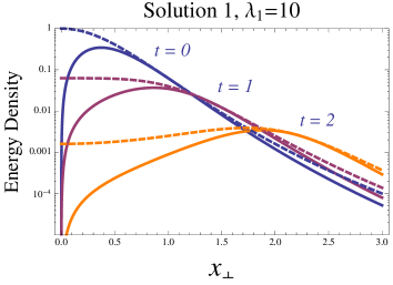
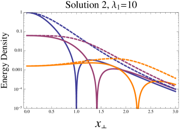
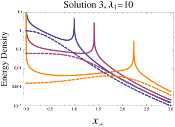
Figure 1: The time-evolution of the energy density profile $\epsilon(x_{\perp})$ at $z=0$ and $t=0,1,2$ for the three solutions in (13). We set $L=1$ and $\lambda_{1}=10$. The dashed lines represent the ideal solution in the limit $\lambda_{1}\to\infty$.

Note that the solutions (13) are invariant under $t\to-t$, that is, they are time-reversible despite $\pi^{\mu\nu}\neq 0$. A simple look at the energy-momentum conservation equations tells us that time reversal invariance is broken if $\pi_{\mu\nu}$ is not even under this operation. In fact, when $t\to-t$ we have that the spatial flow velocity changes as $\vec{u}\to-\vec{u}$, while $\theta\to-\theta$, $\sigma_{\mu\nu}\to-\sigma_{\mu\nu}$. Thus, in the Navier-Stokes approximation $\pi_{\mu\nu}\sim-2\eta\sigma_{\mu\nu}$, one can clearly see that time reversal invariance is broken, which is of course associated with the production of entropy landau . However, our solutions are static in $\tau$ and dissipationless $\hat{\sigma}^{\mu\nu}=\hat{\theta}=0$. Clearly, then, a nontrivial solution of (9) implies that $\hat{\pi}^{\mu\nu}$ is even under time-reversal. Thus, it is indeed possible to find time-reversible fluid configurations in second-order hydrodynamics. Presumably, in the context of kinetic theory, our solutions may correspond to some kind of a nontrivial fixed point of the Boltzmann equation that never reaches local thermal equilibrium. This certainly deserves further study.

In Nagy:2009eq , Nagy also derived an exact ideal-fluid solution with rotation. It is easy to accommodate this solution in our framework. For fluid rotating around the $z$-axis, we just turn on the $\phi$-component of the velocity.

$$\hat{u}_{\tau}=\!\frac{-\cosh^{2}\rho}{\sqrt{\cosh^{2}\rho-\omega^{2}}}\,,\ \hat{u}_{\phi}=\!\frac{\omega}{\sqrt{\cosh^{2}\rho-\omega^{2}}}\,.$$ (14)

with the obvious constraint $1\geq\omega\geq 0$. The corresponding flow velocity in Minkowski space is

$$u_{t} = -\frac{L^{2}+r^{2}+t^{2}}{\sqrt{(L^{2}+t^{2}+r^{2})^{2}-4r^{2}t^{2}-4\omega^{2}L^{2}x_{\perp}^{2}}}\,,$$

$$\vec{u} = \frac{2t\vec{r}+2\omega L(\vec{r}\times\vec{e}_{z})}{\sqrt{(L^{2}+t^{2}+r^{2})^{2}-4r^{2}t^{2}-4\omega^{2}L^{2}x_{\perp}^{2}}}\,,$$ (15)

in agreement with Nagy:2009eq . The modified flow velocity (14) still satisfies $\hat{\theta}=\hat{\sigma}^{\mu\nu}=0$. The energy density is given by

$$\hat{\epsilon}\propto\frac{1}{(\cosh^{2}\rho-\omega^{2})^{2}}\,,$$ (16)

or in Minkowski space,

$$\epsilon\propto\!\frac{1}{((L^{2}+t^{2}+r^{2})^{2}-4r^{2}t^{2}-4\omega^{2}L^{2}x_{\perp}^{2})^{2}}\,.$$ (17)

Naturally, this solution has nonzero vorticity

$$\hat{\Omega}_{\tau\rho}=\!\frac{-\omega^{2}\cosh\rho\sinh\rho}{(\cosh^{2}\rho-\omega^{2})^{3/2}}\,,\ \ \hat{\Omega}_{\phi\rho}\!=\!\frac{\omega\cosh\rho\sinh\rho}{(\cosh^{2}\rho-\omega^{2})^{3/2}}\,.$$

We now include second-order corrections to this solution keeping the flow velocity (14) unchanged. Temporarily assuming $\tau_{\pi}=\lambda_{2}=0$, we find that the solution to (8)

$$\hat{\pi}^{\mu\nu} = \frac{\lambda_{1}}{\hat{\epsilon}}\hat{\pi}^{\langle\mu}_{\ \ \lambda}\hat{\pi}^{\nu\rangle\lambda}+\lambda_{3}\sqrt{\hat{\epsilon}}\,\hat{\Omega}^{\langle\mu}_{\ \ \lambda}\hat{\Omega}^{\nu\rangle\lambda}\,,$$ (18)

is given by

$$(\hat{\pi}^{\rho\rho},\sinh^{2}\rho\hat{\pi}^{\Theta\Theta},\hat{\pi}^{\phi\phi})\!=\!\frac{\hat{\epsilon}}{\lambda_{1}}\left(\alpha,\beta,\frac{\gamma\cosh^{2}\rho}{\cosh^{2}\rho-\omega^{2}}\right)\,,$$

$$\qquad\hat{\pi}^{\tau\tau}=\frac{\omega}{\cosh^{2}\rho}\hat{\pi}^{\tau\phi}=\frac{\omega^{2}}{\cosh^{4}\rho}\hat{\pi}^{\phi\phi}\,.$$ (19)

The parameters $(\alpha,\beta,\gamma)$ in (19) can be any of the following four possibilities

$$(\alpha,\beta,\gamma)\!=\!\begin{cases}\left(\frac{1-\sqrt{9-4f}}{2},-1,\frac{1+\sqrt{9-4f}}{2}\right)\,,\\ \left(\frac{1+\sqrt{9-4f}}{2},-1,\frac{1-\sqrt{9-4f}}{2}\right)\,,\end{cases}$$ (20)

$$\alpha=\gamma=-\frac{\beta}{2}=\begin{cases}\frac{1}{2}\left(-1-\sqrt{1+4f/3}\right)\,,\\ \frac{1}{2}\left(-1+\sqrt{1+4f/3}\right)\,,\end{cases}$$ (21)

where we defined

$$f\equiv\frac{\lambda_{1}\lambda_{3}\omega^{2}\sinh^{2}\rho}{\sqrt{\hat{\epsilon}}(\cosh^{2}\rho-\omega^{2})^{2}}\,.$$ (22)

In the $f\to 0$ limit, the first three solutions in (20)-(21) reduce to (10), while the last solution reduces to the one with $\lambda_{1}=0$. Below we consider only the last two solutions (21) because they satisfy $\hat{\Delta}^{\mu}_{\alpha}\hat{\Delta}^{\nu}_{\beta}\hat{D}\hat{\pi}^{\alpha\beta}=\hat{\pi}^{\langle\mu}_{\ \ \lambda}\hat{\Omega}^{\nu\rangle\lambda}=0$, namely, they are solutions even when $\tau_{\pi},\,\lambda_{2}\neq 0$.

Substituting (19) and (21) into (7), we are left with the following nonlinear differential equation

$$\partial_{\rho}\hat{\epsilon}+\!\frac{4\cosh\rho\sinh\rho}{\cosh^{2}\rho-\omega^{2}}\hat{\epsilon}\!+\!3\!\left[\partial_{\rho}\hat{\pi}^{\rho\rho}\!+\!\frac{4\cosh\rho\sinh\rho}{\cosh^{2}\rho-\omega^{2}}\hat{\pi}^{\rho\rho}\right]$$

$$\qquad\qquad+\frac{9(1-\omega^{2})\coth\rho}{\cosh^{2}\rho-\omega^{2}}\hat{\pi}^{\rho\rho}=0\,.$$ (23)

To solve this, we employ an ansatz

$$\hat{\epsilon}=\frac{A^{2}(\rho)\sinh^{4}\rho}{(\cosh^{2}\rho-\omega^{2})^{4}}\,,$$ (24)

with which we can write $\hat{\pi}^{\rho\rho}=b(\rho)\hat{\epsilon}$ where $b(\rho)$ is the root of

$$A(\rho)=\frac{\lambda_{3}\omega^{2}}{3b(\rho)(\lambda_{1}b(\rho)+1)}\,.$$ (25)

First we find the special solution where $A$ is a constant. In this case, (23) requires either $\omega=1$ or $b=-\frac{4}{21}$. When $\omega=1$, the solution turns out to be the same as the ideal one

$$\hat{\epsilon}=\frac{A^{2}}{\sinh^{4}\rho}\,,$$ (26)

where $A$ is arbitrary. On the other hand, when $b=-\frac{4}{21}$,

$$A=\frac{7\lambda_{3}\omega^{2}}{4\left(\frac{4}{21}\lambda_{1}-1\right)}\,,$$ (27)

is the solution. Note that if we take the limits $\omega\to 0$ and $\lambda_{1}\to\frac{21}{4}$ in (27) such that $A$ remains finite, (24) reduces to the second solution in (12).

To find general solutions, we now take into account the $\rho$-dependence of $A(\rho)$. (23) can be cast into a differential equation for $b(\rho)$

$$\frac{9\lambda_{1}b^{2}+4\lambda_{1}b+3b+2}{b(\lambda_{1}b+1)(4+21b)}\partial_{\rho}b=\frac{(1-\omega^{2})\coth\rho}{\cosh^{2}\rho-\omega^{2}}\,.$$ (28)

The above equation can be integrated as

$$b\left(21b+4\right)^{e_{1}}\left(\lambda_{1}b+1\right)^{e_{2}}=\textrm{C}\frac{\sinh^{2}\rho}{\cosh^{2}\rho-\omega^{2}}\,,$$ (29)

where $e_{1}=\frac{105-32\lambda_{1}}{7(4\lambda_{1}-21)}$, $e_{2}=1+\frac{9}{4\lambda_{1}-21}$ and C is the integration constant. Given $b^{\ast}(\rho)$ as the solution to (29), we can obtain the energy density accordingly. In the limit $\lambda_{1}\to\infty$, (29) indicates that $b\to 0$, and we recover the ideal solution (16).

In conclusion, we have found several novel exact solutions to the second-order conformal hydrodynamic equations in which $\pi^{\mu\nu}$ is treated as independent variable. The ideal-fluid limit of these solutions reduces to previously known results. Our solutions encode very interesting nonlinear effect as well as the vorticity contribution, which has never been studied before. We showed that the second-order equations allow for nontrivial time-reversible solutions in which $\pi^{\mu\nu}$ cannot be approximated by its Navier-Stokes limit. Although these solutions are rather special, they cannot be ruled out as nonphysical simply using the second law of thermodynamics. We hope that the new solutions described here may not only shed new light on the analytical structure of the nonlinear second-order hydrodynamic equations but also serve as a test of numerical codes for the hydrodynamic simulation of heavy-ion collisions.

Acknowledgements—The authors thank the Yukawa Institute for Theoretical Physics, Kyoto University, where this collaboration started during the YITP-T-13-05 workshop “New Frontiers in QCD”. We thank helpful conversations with the participants of this workshop. J. N. thanks G. S. Denicol for enlightening discussions and Conselho Nacional de Desenvolvimento Científico e Tecnológico (CNPq) and Fundação de Amparo à Pesquisa do Estado de São Paulo (FAPESP) for financial support.

References

• (1) U. Heinz and R. Snellings, Ann. Rev. Nucl. Part. Sci.  63, 123 (2013) [arXiv:1301.2826 [nucl-th]].
• (2) S. R. De Groot, W. A. Van Leeuwen and C. G. Van Weert, “Relativistic Kinetic Theory. Principles and Applications,” Amsterdam, Netherlands: North-holland ( 1980) 417p
• (3) R. Baier, P. Romatschke, D. T. Son, A. O. Starinets and M. A. Stephanov, JHEP 0804, 100 (2008) [arXiv:0712.2451 [hep-th]].
• (4) S. Bhattacharyya, V. E. Hubeny, S. Minwalla and M. Rangamani, JHEP 0802, 045 (2008) [arXiv:0712.2456 [hep-th]].
• (5) T. Koide, G. S. Denicol, P. .Mota and T. Kodama, Phys. Rev. C 75, 034909 (2007) [hep-ph/0609117].
• (6) J. Peralta-Ramos and E. Calzetta, Phys. Rev. D 80, 126002 (2009) [arXiv:0908.2646 [hep-ph]].
• (7) G. S. Denicol, J. Noronha, H. Niemi and D. H. Rischke, Phys. Rev. D 83, 074019 (2011) [arXiv:1102.4780 [hep-th]].
• (8) G. S. Denicol, H. Niemi, E. Molnar and D. H. Rischke, Phys. Rev. D 85, 114047 (2012) [arXiv:1202.4551 [nucl-th]].
• (9) K. Tsumura and T. Kunihiro, Eur. Phys. J. A 48, 162 (2012) [arXiv:1206.1929 [nucl-th]].
• (10) W. Israel and J. M. Stewart, Annals Phys.  118, 341 (1979).
• (11) M. Luzum and P. Romatschke, Phys. Rev. C 78, 034915 (2008) [Erratum-ibid. C 79, 039903 (2009)] [arXiv:0804.4015 [nucl-th]].
• (12) J. D. Bjorken, Phys. Rev. D 27, 140 (1983).
• (13) T. S. Biro, Phys. Lett. B 487, 133 (2000) [nucl-th/0003027].
• (14) T. Csorgo, F. Grassi, Y. Hama and T. Kodama, Phys. Lett. B 565, 107 (2003) [nucl-th/0305059].
• (15) T. Csorgo, M. I. Nagy and M. Csanad, Phys. Lett. B 663, 306 (2008) [nucl-th/0605070].
• (16) A. Bialas, R. A. Janik and R. B. Peschanski, Phys. Rev. C 76, 054901 (2007) [arXiv:0706.2108 [nucl-th]].
• (17) G. Beuf, R. Peschanski and E. N. Saridakis, Phys. Rev. C 78, 064909 (2008) [arXiv:0808.1073 [nucl-th]].
• (18) I. Fouxon and Y. Oz, JHEP 0903, 120 (2009) [arXiv:0812.1266 [hep-th]].
• (19) M. I. Nagy, Phys. Rev. C 83, 054901 (2011) [arXiv:0909.4285 [nucl-th]].
• (20) J. Liao and V. Koch, Phys. Rev. C 80, 034904 (2009) [arXiv:0905.3406 [nucl-th]].
• (21) S. S. Gubser, Phys. Rev. D 82, 085027 (2010) [arXiv:1006.0006 [hep-th]].
• (22) S. S. Gubser and A. Yarom, Nucl. Phys. B 846, 469 (2011) [arXiv:1012.1314 [hep-th]].
• (23) H. Marrochio, J. Noronha, G. S. Denicol, M. Luzum, S. Jeon and C. Gale, arXiv:1307.6130 [nucl-th].
• (24) $AdS_{3}$ is the space satisfying $X_{0}^{2}-X_{1}^{2}-X_{2}^{2}+X_{3}^{2}=L^{2}$. The Poincaré coordinates shown in (1) are obtained by the parametrization $X_{0}=\frac{t}{x_{\perp}}L$, $X_{1}=\frac{z}{x_{\perp}}L$, $X_{2}=\frac{L^{2}-r^{2}+t^{2}}{2x_{\perp}}\,$, $X_{3}=\frac{L^{2}+r^{2}-t^{2}}{2x_{\perp}}$. The global coordinates are obtained by $X_{0}=L\cosh\rho\cos\tau\,$, $X_{1}=L\sinh\rho\sin\Theta\,$, $X_{2}=L\sinh\rho\cos\Theta\,$, $X_{3}=L\cosh\rho\sin\tau$.
• (25) L. D. Landau and E. M. Lifshitz, Fluid Mechanics, Second Edition: Volume 6 (Course of Theoretical Physics), Butterworth-Heinemann, 1987.