Phenomenological discriminations of the Yukawa interactions in two-Higgs doublet models with $Z_{2}$ symmetry

Abstract

There are four types of two-Higgs doublet models under a discrete $Z_{2}$ symmetry imposed to avoid tree-level flavour-changing neutral current, i.e. type-I, type-II, type-X and type-Y models. We investigate the possibility to discriminate the four models in the light of the flavour physics data, including $B_{s}-\bar{B}_{s}$ mixing, $B_{s,d}\to\mu^{+}\mu^{-}$, $B\to\tau\nu$ and $\bar{B}\to X_{s}\gamma$ decays, the recent LHC Higgs data, the direct search for charged Higgs at LEP, and the constraints from perturbative unitarity and vacuum stability. After deriving the combined constraints on the Yukawa interaction parameters, we have shown that the correlation between the mass eigenstate rate asymmetry $A_{\Delta\Gamma}$ of $B_{s}\to\mu^{+}\mu^{-}$ and the ratio $R={\cal B}(B_{s}\to\mu^{+}\mu^{-})_{\rm exp}/{\cal B}(B_{s}\to\mu^{+}\mu^{-})_{\rm SM}$ could be a sensitive probe to discriminate the four models with future precise measurements of the observables in the $B_{s}\to\mu^{+}\mu^{-}$ decay at LHCb.

1 Introduction

Although the Standard Model (SM) for particle physics has been successful for over three decades, it still shows some problems which solutions could imply physics beyond its scope [1, 2, 3, 4, 5, 6, 7, 8, 9, 10]. Recently, the ATLAS [11, 12] and CMS [13, 14] experiments at LHC have discovered a new neutral boson with properties consistent with those of the SM Higgs boson [15, 16, 17, 18, 19, 20]. With the experimental progress at LHC, it is of great interest to confirm whether this boson is the only one fundamental scalar just as the SM, or belongs to an extended scalar sector responsible to the electroweak symmetry breaking (EWSB). The simplest scenario entertaining the latter possibility is provided by the two-Higgs doublet models (2HDM).

Besides the SM Higgs sector, an additional Higgs doublet is introduced in the 2HDMs. This class of models can provide new source of CP violation beyond the SM [21], which are needed to explain the observed cosmic matter-antimatter asymmetry. The 2HDMs could also be understood as an effective theory for many natural EWSB scenarios, such as the Minimal Supersymmetric Standard Model (MSSM) [22].

However, unlike the SM, the tree-level flavour-changing neutral current (FCNC) transition in the 2HDM is not forbidden by the Glashow-Iliopoulos-Maiani (GIM) mechanism. These FCNCs can cause severe phenomenological difficulties [23, 24, 25]. Besides some other solutions [26, 27, 28, 29, 30], this problem can be addressed by imposing a discrete $Z_{2}$ symmetry [31]. According to different $Z_{2}$ charge assignments, there are four types of 2HDMs, referred to, respectively, as the type-I, type-II, type-X and type-Y 2HDMs [32]. Therefore, phenomenologically distinguishing between these 2HDMs is an important issue and worthy of detailed investigation [33].

The 2HDMs present very interesting phenomena in both low-energy flavour transitions such as $B\to X_{s}\gamma$ decay and $B_{s}-\bar{B}_{s}$ mixing, and high-energy collider processes such as various Higgs decay channels. At present, many analyses have been performed [39, 45, 43, 38, 50, 44, 47, 40, 35, 37, 46, 42, 34, 48, 41, 49, 36], however, most of them concentrate on the type-II 2HDM. In this work, we shall extend the previous analyses and study the possibility to discriminate the four different types of 2HDM in favor of experimental measurement. To constrain the model parameters, we shall consider the following constraints:

• flavour processes: $B_{s}-\bar{B}_{s}$ mixing, $\bar{B}\to X_{s}\gamma$, $B\to\tau\nu$ and $B_{s,d}\to\mu^{+}\mu^{-}$ decays,

• direct search for Higgs bosons at LEP, Tevatron, and LHC,

• perturbative unitarity and vacuum stability.

For the $B_{s}\to\mu^{+}\mu^{-}$ decay, there are several interesting observables very sensitive to new physics effects as suggested recently by De Bruyn et al. [51]. In this paper, we use these observables to probe the 2HDMs and find the correlation between the mass eigenstate rate asymmetry $A_{\Delta\Gamma}$ and the ratio $R={\cal B}(B_{s}\to\mu^{+}\mu^{-})_{\rm exp}/{\cal B}(B_{s}\to\mu^{+}\mu^{-})_{\rm SM}$, which could be used to discriminate the four models with future precise measurements of the observables in the $B_{s}\to\mu^{+}\mu^{-}$ decay at LHCb.

Our paper is organized as follows: In the next section, we give a brief review on the 2HDM with the $Z_{2}$ symmetry. In section 3, the theoretical formalism for the flavour observables are presented. In section 4, we give our detailed numerical results and discuss the possibility of discriminating the four types of 2HDM. Our conclusions are given in section 5. The relevant Wilson coefficients due to the contributions of 2HDMs are presented in the appendices A and B.

2 2HDM under the $Z_{2}$ symmetry

In the 2HDM, the two Higgs doublets $\Phi_{1}$ and $\Phi_{2}$ can be generally parameterized as

$$\Phi_{i}=\begin{pmatrix}\omega_{i}^{+}\\ \frac{1}{\sqrt{2}}(v_{i}+h_{i}-iz_{i})\end{pmatrix}.$$ (2.1)

For a CP-conserving Higgs potential, the two vacuum expectation values (vevs) $v_{1}$ and $v_{2}$ are real and positive  [22]. They satisfy the relations $v_{1}=v\cos\beta$ and $v_{2}=v\sin\beta$ with $v=246\,\rm GeV$. The physical scalars can be obtained by the rotations

$$\begin{pmatrix}h_{1}\\ h_{2}\end{pmatrix}=R(\alpha)\begin{pmatrix}H\\ h\end{pmatrix},\quad\begin{pmatrix}z_{1}\\ z_{2}\end{pmatrix}=R(\beta)\begin{pmatrix}z\\ A\end{pmatrix},\quad\begin{pmatrix}\omega_{1}^{+}\\ \omega_{2}^{+}\end{pmatrix}=R(\beta)\begin{pmatrix}\omega^{+}\\ H^{+}\end{pmatrix},$$ (2.2)

where the rotation matrix is given by

$$R(\theta)=\begin{pmatrix}\cos\theta&-\sin\theta\\ \sin\theta&\cos\theta\end{pmatrix}.$$ (2.3)

The mixing angles $\alpha$ and $\beta$ are determined by the parameters of the Higgs potential. The physical Higgs spectrum consists of five degrees of freedom: two charged scalars $H^{\pm}$, two CP-even neutral scalars $h$ and $H$, and one CP-odd neutral scalar $A$.

In the interaction basis, the Yukawa interactions of these Higgs bosons can be written as

$$-\mathcal{L}_{Y}=\bar{Q}_{L}(Y_{1}^{d}\Phi_{1}+Y_{2}^{d}\Phi_{2})d_{R}+\bar{Q}_{L}(Y_{1}^{u}\tilde{\Phi}_{1}+Y_{2}^{u}\tilde{\Phi}_{2})u_{R}+\bar{L}_{L}(Y_{1}^{\ell}\Phi_{1}+Y_{2}^{\ell}\Phi_{2})e_{R}+\text{H.c.},$$ (2.4)

where $\tilde{\Phi}_{i}=i\sigma_{2}\Phi_{i}^{*}$ with $\sigma_{2}$ the Pauli matrix, $Q_{L}$ and $L_{L}$ denote the left-handed quark and lepton doublets, and $u_{R}$, $d_{R}$ and $e_{R}$ are the right-handed up-type quark, down-type quark and lepton singlet, respectively. The Yukawa coupling matrices $Y_{i}^{f}$ ($f=u,d,\ell$) are $3\times 3$ complex matrices in flavour space.

	$\Phi_{1}$	$\Phi_{2}$	$u_{R}$	$d_{R}$	$\ell_{R}$	$Q_{L}$, $L_{L}$
Type-I	$+$	$-$	$-$	$-$	$-$	$+$
Type-II	$+$	$-$	$-$	$+$	$+$	$+$
Type-X	$+$	$-$	$-$	$-$	$+$	$+$
Type-Y	$+$	$-$	$-$	$+$	$-$	$+$

Table 1: Charge assignments of the $Z_{2}$ symmetry in the four types of 2HDM.

	$\xi_{h}^{u}$	$\xi_{h}^{d}$	$\xi_{h}^{\ell}$	$\xi_{H}^{u}$	$\xi_{H}^{d}$	$\xi_{H}^{\ell}$	$\xi_{A}^{u}$	$\xi_{A}^{d}$	$\xi_{A}^{\ell}$
Type-I	$c_{\alpha}/s_{\beta}$	$+c_{\alpha}/s_{\beta}$	$+c_{\alpha}/s_{\beta}$	$s_{\alpha}/s_{\beta}$	$s_{\alpha}/s_{\beta}$	$s_{\alpha}/s_{\beta}$	$-\cot\beta$	$+\cot\beta$	$+\cot\beta$
Type-II	$c_{\alpha}/s_{\beta}$	$-s_{\alpha}/c_{\beta}$	$-s_{\alpha}/c_{\beta}$	$s_{\alpha}/s_{\beta}$	$c_{\alpha}/c_{\beta}$	$c_{\alpha}/c_{\beta}$	$-\cot\beta$	$-\tan\beta$	$-\tan\beta$
Type-X	$c_{\alpha}/s_{\beta}$	$+c_{\alpha}/s_{\beta}$	$-s_{\alpha}/c_{\beta}$	$s_{\alpha}/s_{\beta}$	$s_{\alpha}/s_{\beta}$	$c_{\alpha}/c_{\beta}$	$-\cot\beta$	$+\cot\beta$	$-\tan\beta$
Type-Y	$c_{\alpha}/s_{\beta}$	$-s_{\alpha}/c_{\beta}$	$+c_{\alpha}/s_{\beta}$	$s_{\alpha}/s_{\beta}$	$c_{\alpha}/c_{\beta}$	$s_{\alpha}/s_{\beta}$	$-\cot\beta$	$-\tan\beta$	$+\cot\beta$

Table 2: Yukawa couplings in the four types of 2HDM.

In order to avoid tree-level FCNC, it is natural to introduce a discrete $Z_{2}$ symmetry [31]. All the possible nontrivial $Z_{2}$ charge assignments are listed in table 1, which define the four well-known types of 2HDM, i.e. type-I, type-II, type-X and type-Y. The Yukawa interactions in the four models are different. In the mass-eigenstate basis, they can be unified in the form

$$-{\mathcal{L}}_{Y}= +\sum_{f=u,d,\ell}\left[m_{f}\bar{f}f+\left(\frac{m_{f}}{v}\xi_{h}^{f}\bar{f}fh+\frac{m_{f}}{v}\xi_{H}^{f}\bar{f}fH-i\frac{m_{f}}{v}\xi_{A}^{f}\bar{f}\gamma_{5}fA\right)\right]$$

$$+\frac{\sqrt{2}}{v}\bar{u}\left(m_{u}V\xi_{A}^{u}P_{L}+Vm_{d}\xi_{A}^{d}P_{R}\right)dH^{+}+\frac{\sqrt{2}m_{\ell}\xi_{A}^{\ell}}{v}\bar{\nu}_{L}\ell_{R}H^{+}+\text{H.c.},$$ (2.5)

where $P_{L,R}=(1\pm\gamma_{5})/2$ and $V$ denotes the Cabibbo-Kobayashi-Maskawa (CKM) matrix. The couplings $\xi_{h,H,A}^{f}$ in the four types of 2HDM are listed in table 2.

3 Theoretical formalism for flavour observables

In this section, we shall recapitulate the basic theoretical formulae for the relevant B-meson decay and mixing processes and discuss the contributions of the four types of 2HDMs.

3.1 $B_{s}-\bar{B}_{s}$ mixing

For the $B_{s}-{\bar{B}}_{s}$ mixing, the mass difference is defined as

$$\Delta m_{B_{s}}=m_{H}-m_{L},$$ (3.1)

where $H$ and $L$ denote the heavy and light mass eigenstates. This quantity arises from $W$ box diagrams in the SM and can receive contributions from Higgs box diagrams in 2HDM, as shown in figure 1. The theoretical prediction can be expressed as [52, 53, 54]

Figure 1: Box diagrams for the $B_{s}-\bar{B}_{s}$ mixing in the SM and 2HDM.

$$\Delta m_{B_{s}}=\frac{G_{F}^{2}}{6\pi^{2}}m_{W}^{2}|V_{tb}V_{ts}^{*}|^{2}S(x_{t},x_{H^{\pm}})\hat{\eta}_{B_{s}}\mathcal{B}_{B_{s}}(m_{b})f^{2}_{B_{s}}m_{B_{s}},$$ (3.2)

with the definitions $x_{t}\equiv({{\overline{m}}_{t}({\overline{m}}_{t})})^{2}/m_{W}^{2}$ and $x_{H^{\pm}}\equiv{{m}}_{H^{\pm}}^{2}/m_{W}^{2}$. The long-distance QCD effects are contained in the bag factor $\mathcal{B}_{B_{s}}(m_{b})$ and the decay constant $f_{B_{s}}$ [52]. The short-distance contributions from the SM and 2HDM are encoded in the Inami-Lim function $S(x_{t},x_{H^{\pm}})$, with its explicit expression given in appendix A, and the QCD correction factor $\hat{\eta}_{B_{s}}$.

3.2 $\bar{B}\to X_{s}\gamma$ decay

The effective Hamiltonian for $\bar{B}\rightarrow X_{s}\gamma$ at the scale $\mu_{b}={\mathcal{O}}(m_{b})$ is given as follows [55, 56, 57, 58, 59, 60, 61]

Figure 2: One-loop diagrams contributing to $\bar{B}\to X_{s}\gamma$ through the $W$ boson and the charged Higgs boson exchange in the SM and 2HDM, respectively.

$$\mathcal{H}_{\rm eff}=-\frac{G_{F}}{\sqrt{2}}V_{ts}^{\ast}V_{tb}\left(\sum\limits_{i=1}^{6}C_{i}(\mu_{b})Q_{i}+C_{7\gamma}(\mu_{b})Q_{7\gamma}+C_{8g}(\mu_{b})Q_{8g}\right),$$ (3.3)

where $Q_{1-6}$ are the four-fermion operators whose explicit expressions are given in ref. [58]. The remaining magnetic-penguin operators, which are characteristic for this decay, are defined as

$$Q_{7\gamma}=\frac{e}{8\pi^{2}}m_{b}\bar{s}_{\alpha}\sigma^{\mu\nu}(1+\gamma_{5})b_{\alpha}F_{\mu\nu},\qquad Q_{8g}=\frac{g_{s}}{8\pi^{2}}m_{b}\bar{s}_{\alpha}\sigma^{\mu\nu}(1+\gamma_{5})T^{a}_{\alpha\beta}b_{\beta}G_{\mu\nu}^{a},$$ (3.4)

where $m_{b}$ denotes the $b$-quark mass in the $\rm\overline{MS}$ scheme, and $e$ ($g_{s}$) is the electromagnetic (strong) coupling constant. The Wilson coefficients $\{C_{i}\}$ can be calculated perturbatively. In 2HDM, the photon-penguin diagrams mediated by charged Higgs, as shown in figure 2, result in the following derivations:

$$C_{7\gamma}=C_{7\gamma}^{\text{SM}}+C_{7\gamma}^{\text{2HDM}},\qquad C_{8g}=C_{8g}^{\text{SM}}+C_{8g}^{\text{2HDM}}.$$ (3.5)

In the SM and the four types of 2HDM, analytic expressions for the Wilson coefficients up to the next-to-leading order (NLO) are given in refs. [59, 60]. The next-to-next-leading order (NNLO) SM and 2HDM calculation can be found in ref. [62] and ref. [44], respectively.

The branching ratio of $\bar{B}\rightarrow X_{s}\gamma$ with an energy cut-off $E_{0}$ can be expressed as

$${\mathcal{B}}(\bar{B}\rightarrow X_{s}\gamma)_{{E_{\gamma}}\geq E_{0}}={\mathcal{B}}(\bar{B}\rightarrow X_{c}e\bar{\nu})_{\rm exp}{{\bigg{\lvert}}\frac{V_{ts}^{*}V_{tb}}{V_{cb}}{\bigg{\rvert}}}^{2}\frac{6\alpha_{e}}{\pi C}[P(E_{0})+N(E_{0})],$$ (3.6)

with the semi-leptonic factor

$$C={\left\lvert\frac{V_{ub}}{V_{cb}}\right\rvert}^{2}\frac{\Gamma(\bar{B}\to X_{c}e\bar{\nu})}{\Gamma(\bar{B}\to X_{u}e\bar{\nu})}.$$ (3.7)

The perturbative quantity $P(E_{0})$, which is expressed in terms of Wilson coefficients, and the non-perturbative correction $N(E_{0})$ can be found in ref. [59].

3.3 $B\to\tau\nu$ decay

The tauonic decay $B\to\tau\nu$ is described as annihilation processes mediated by $W$ boson in the SM and the charged Higgs boson in 2HDM, as shown in figure 3. Therefore, this process is very sensitive to the charged Higgs boson $H^{\pm}$ and provides an important constraint on the model parameters.

Within 2HDM, the decay width of this channel reads [32, 63, 64],

$$\Gamma(B\to\tau\nu)=\frac{G_{F}^{2}{{\left|V_{ub}\right|}^{2}}}{8\pi}f_{B}^{2}m_{B}m_{\tau}^{2}{{\left(1-\frac{m_{\tau}^{2}}{m_{B}^{2}}\right)}^{2}}{{\left(1-\frac{m_{B}^{2}}{m_{H^{\pm}}^{2}}\xi_{A}^{d}\xi_{A}^{\ell}\right)}^{2}},$$ (3.8)

where $V_{ub}$ is the CKM matrix element and $f_{B}$ denotes the B-meson decay constant.

Figure 3: Tree-level diagrams contributing to $B\to\tau\nu_{\tau}$ in the SM and 2HDM.

3.4 $B_{s,d}\to\mu^{+}\mu^{-}$ decay

In the SM, the $B_{q}\to\mu^{+}\mu^{-}$ decays ($q=d\text{ or }s$) arise from the $W$ box and $Z$ penguin diagrams at the quark level [65, 66], as shown in figure 4. The helicity suppression in these decays may be relaxed by NP contributions, which can significantly enhance their branching ratios. Generally, the low-energy effective Hamiltonian for $B_{q}\to\mu^{+}\mu^{-}$ decay can be written as  [67]

$$\mathcal{H}_{\rm eff}=\frac{G_{F}}{\sqrt{2}}\frac{\alpha_{e}}{2\pi s_{W}}V_{tb}^{\ast}V_{tq}\left(C_{S}Q_{S}+C_{P}Q_{P}+C_{A}Q_{A}\right),$$ (3.9)

with $s_{W}\equiv\sin\theta_{W}$. The semi-leptonic operators are defined as

$$Q_{S}=m_{b}(\bar{b}P_{L}q)(\bar{\mu}\mu),\qquad Q_{P}=m_{b}(\bar{b}P_{L}q)(\bar{\mu}\gamma_{5}\mu),\qquad Q_{A}=(\bar{b}\gamma^{\mu}P_{L}q)(\bar{\mu}\gamma_{\mu}\gamma_{5}\mu).$$ (3.10)

Among the Wilson coefficients $C_{S,P,A}$, only $C_{A}$ is non-zero in the SM. Its explicit expressions up to NLO can be found in refs. [68, 69, 70]. Recently, the NLO EW [71] and NNLO QCD [72] corrections have also been completed [73]. In the 2HDM, $C_{A}$ is not affected, whereas $C_{S,P}$ receive contributions from both charged and neutral Higgs bosons. At present, only the diagrams shown in figure 4 have been calculated in the type-II 2HDM with large $\tan\beta$ [67]. Based on these results, we give the Wilson coefficients $C_{S,P}$ corresponding to these diagrams in all the four types of 2HDM with arbitrary $\tan\beta$ in appendix B. It is noted that contributions from other diagrams may be important for some specific values of $\tan\beta$ (large or small) and will become crucial with future high-precision measurement of $B_{q}\to\mu^{+}\mu^{-}$ decays.

For $B_{q}\to\mu^{+}\mu^{-}$ decays, one important observable is the CP averaging branching ratio, which reads

$$\mathcal{B}(B_{q}\to\mu^{+}\mu^{-})=\frac{G_{F}^{2}{\alpha_{e}^{2}}}{32\pi^{2}s_{W}^{4}}\frac{m_{B_{q}}^{3}\tau_{B_{q}}f_{B_{q}}^{2}}{8\pi}\sqrt{1-\frac{4m_{\mu}^{2}}{m_{B_{q}}^{2}}}\left(\frac{2m_{\mu}}{m_{B_{q}}}\right)^{2}\left\lvert V_{tb}V_{tq}^{*}\right\rvert^{2}\left\lvert C_{A}\right\rvert^{2}(\left\lvert S\right\rvert^{2}+\left\lvert P\right\rvert^{2}),$$ (3.11)

with the definitions

$$P\equiv 1-\frac{m_{B_{q}}^{2}}{2m_{\mu}}\frac{C_{P}^{\ast}}{C_{A}^{\ast}},\qquad S\equiv\sqrt{1-4\frac{m_{\mu}^{2}}{m_{B_{q}}^{2}}}\frac{m_{B_{q}}^{2}}{2m_{\mu}}\frac{C_{S}^{\ast}}{C_{A}^{\ast}}.$$ (3.12)

It is noted that the contributions of the $C_{S,P}$ terms do not suffer helicity suppression, but they are suppressed by the small leptonic Yukawa coupling in the 2HDMs. However, they may be enhanced by a large $\tan\beta$ (or $\cot\beta$) factor [65, 66, 68, 69, 67].

Figure 4: Dominant SM and 2HDM diagrams for the $B_{s}\to\mu^{+}\mu^{-}$ decays.

Recently, a sizable width difference $\Delta\Gamma_{s}$ between the $B_{s}$ mass eigenstates has been measured at the LHCb [74]

$$y_{s}\equiv\frac{\Gamma_{s}^{\rm L}-\Gamma_{s}^{\rm H}}{\Gamma_{s}^{\rm L}+\Gamma_{s}^{\rm H}}=\frac{\Delta\Gamma_{s}}{2\Gamma_{s}}=0.080\pm 0.010,$$ (3.13)

where $\Gamma_{s}$ denotes the inverse of the $B_{s}$ mean lifetime $\tau_{B_{s}}$. As pointed out in ref. [51], the measured branching ratio of $B_{q}\to\mu^{+}\mu^{-}$ should be the time-integrated one, denoted by $\overline{\mathcal{B}}(B_{q}\to\mu^{+}\mu^{-})$. For $B_{s}\to\mu^{+}\mu^{-}$ decay, in order to compare with the experimental measurement, the sizable width difference effect should be taken into account in the theoretical prediction, and one has

$$\overline{{\mathcal{B}}}({{{B}}_{s}}\to\mu^{+}\mu^{-})=\left[\frac{1+A_{\Delta\Gamma}y_{s}}{1-y_{s}^{2}}\right]{\mathcal{B}}({{{B}}_{s}}\to\mu^{+}\mu^{-}),$$ (3.14)

where $A_{\Delta\Gamma}$ denotes the mass eigenstate rate asymmetry, which can be expressed as

$$A_{\Delta\Gamma}=\frac{|P|^{2}\cos 2\varphi_{P}-|S|^{2}\cos 2\varphi_{S}}{|P|^{2}+|S|^{2}},$$ (3.15)

where $\varphi_{P}$ and $\varphi_{S}$ denote the phase of the quantity $P$ and $S$, respectively. In the four types of 2HDM, $\varphi_{P}=\varphi_{S}=0$. The observable $A_{\Delta\Gamma}$ is complementary to the branching ratio of $B_{s}\to\mu^{+}\mu^{-}$, offering independent information on the short-distance structure of this decay. It can be extracted from the time-dependent untagged decay rate [51, 75]. In the SM, $A_{\Delta\Gamma}=+1$. In addition, since the finite width difference in the $B_{d}$ system is negligible, the approximation $\overline{\mathcal{B}}(B_{d}\to\mu^{+}\mu^{-})\approx{\mathcal{B}}(B_{d}\to\mu^{+}\mu^{-})$ works well.

Following ref. [51], it is convenient to introduce the ratio

$$R\equiv\frac{\overline{{\mathcal{B}}}(B_{s}\rightarrow\mu^{+}\mu^{-})}{{\mathcal{B}}(B_{s}\rightarrow\mu^{+}\mu^{-})_{\text{SM}}}=\frac{1+y_{s}\cos 2\varphi_{P}}{1-y_{s}^{2}}|P|^{2}+\frac{1-y_{s}\cos 2\varphi_{S}}{1-y_{s}^{2}}|S|^{2},$$ (3.16)

where $\varphi_{P}=\varphi_{S}=0$ in the four types of 2HDM.

It is also useful to define the following quantity:

$$R_{sd}\equiv\frac{\overline{{\mathcal{B}}}(B_{s}\to\mu^{+}\mu^{-})}{\overline{{\mathcal{B}}}(B_{d}\rightarrow\mu^{+}\mu^{-})},$$ (3.17)

in which some uncertainties of input parameters are canceled out. For example, the $f_{B_{s}}/f_{B_{d}}$ in the above ratio can be directly determined by Lattice QCD and the corresponding theoretical uncertainty is significantly reduced [76, 77].

4 Numerical analysis and discussions

With the theoretical framework presented in the previous sections, we proceed to present our numerical results and discussion in this section.

$V_{us}$	$0.22537\pm 0.00063$	[78]	$s_{W}^{2}$	$0.23116\pm 0.00012$	[79]
$V_{ub}$	$(0.00399\pm 0.00055)e^{i(-71.1\pm 5.1)^{\circ}}$	[78]	$\alpha_{s}(m_{Z})$	$0.1184\pm 0.0007$	[79]
$V_{cb}$	$0.04071\pm 0.00096$	[78]	$\alpha_{e}(m_{Z})^{-1}$	$127.944\pm 0.014$	[79]
$V_{td}$	$(0.00872\pm 0.00041)e^{i(-24.6\pm 2.7)^{\circ}}$	[78]	$f_{B_{s}}$	$(227.6\pm 5.0)\,\text{MeV}$	[80]
$V_{ts}$	$(-0.03998\pm 0.00094)e^{i(1.19\pm 0.11)^{\circ}}$	[78]	$f_{B_{d}}$	$(190.6\pm 4.7)\,\text{MeV}$	[80]
$V_{tb}$	$0.999163\pm 0.000039$	[78]	$f_{B_{s}}/f_{B_{d}}$	$1.201\pm 0.017$	[80]
$\overline{m}_{s}(\overline{m}_{b})$	$(0.085\pm 0.017)\,\text{GeV}$	[52]	${\mathcal{B}}_{B_{s}}(m_{b})$	$0.841\pm 0.024$	[52]
${\overline{m}}_{c}({\overline{m}}_{c})$	$(1.275\pm 0.025)\,\text{GeV}$	[79]	$\hat{\eta}_{B}$	$0.8393\pm 0.0034$	[52]
$\overline{m}_{b}(\overline{m}_{b})$	$(4.248\pm 0.051)\,\text{GeV}$	[52]	$\mathcal{B}(\bar{B}\to X_{c}e\bar{\nu})$	$0.101\pm 0.004$	[79]
$m_{t}^{\text{pole}}$	$(173.5\pm 0.6\pm 0.8)\,\text{GeV}$	[79]	$m_{b}^{\rm 1S}$	$(4.65\pm 0.03)\,\text{GeV}$	[79]

Table 3: The relevant input parameters used in the numerical analysis. The meson masses and lifetimes can be found in ref. [79].

4.1 SM predictions and experimental data

4.1.1 Flavour observables within the SM

Within the SM, our predictions for the flavour observables as well as the corresponding experimental data are collected in table 4. The theoretical uncertainties are obtained by varying the input parameters listed in table 3 within their respective ranges and adding them in quadrature. It is noted that, taking into account the theoretical uncertainties, our SM predictions are in good agreement with the current data. The only tension appears in the branching ratio of $B_{d}\to\mu^{+}\mu^{-}$, which however has a rather large experimental error. Thus, strong constraints on the four types of 2HDM and good discrimination between them are excepted.

Observable	SM prediction	Experiment	Ref.
$\Delta m_{B_{s}}$ [$10^{-11}\,\rm GeV$]	$1.100_{-0.077}^{+0.079}$	$1.164\pm 0.005$	[79]
${\mathcal{B}}(B\to\tau\nu_{\tau})$ [$10^{-4}$]	$1.02_{-0.27}^{+0.31}$	$1.65\pm 0.34$	[79]
${\mathcal{B}}(\bar{B}\to X_{s}\gamma)$ [$10^{-4}$]	$3.16\pm 0.26$	$3.43\pm 0.22$	[81]
$\overline{{\mathcal{B}}}(B_{d}\to\mu^{+}\mu^{-})$ [$10^{-10}$]	$1.16_{-0.12}^{+0.13}$	$3.6_{-1.4}^{+1.6}$	[82, 83, 84]
$\overline{{\mathcal{B}}}(B_{s}\to\mu^{+}\mu^{-})$ [$10^{-9}$]	$3.76_{-0.25}^{+0.26}$	$2.9\pm 0.7$	[82, 83, 84]
$R_{sd}$	$32.84_{-3.81}^{+3.45}$
$R$	$1.08\pm 0.01$	$0.86\pm 0.21$	[83, 84]

Table 4: SM predictions and experimental data for the flavour observables. For the inclusive $\bar{B}\to X_{s}\gamma$ decay, the value given here corresponds to a photon energy cut at $E_{0}=1.6\,\rm GeV$.

4.1.2 Direct search for the Higgs bosons

Direct searches for charged Higgs bosons motivated by 2HDM have been performed at LEP [85], Tevatron [86, 87] and LHC [88, 89]. However, the obtained limits on the charged-Higgs mass depend strongly on the assumed Yukawa structure. In type-II 2HDM, the parameter space with $m_{H^{\pm}}<m_{t}$ is almost excluded by the ATLAS [88], which, however, can not be readily translated into constraints on the parameters of other 2HDMs. Without assumptions on the Yukawa structure, the LEP collaboration established the bound on the charged Higgs boson mass [85]

$$m_{H^{\pm}}\geq 79.3\,\text{GeV},$$

in which $\mathcal{B}(H^{+}\to\tau^{+}\nu_{\tau})+\mathcal{B}(H^{+}\to c\bar{s})=1$ is assumed. In addition, the hadronic $Z\to b\bar{b}$ branching ratio $R_{b}$ can also set indirect limits on $m_{H^{\pm}}$. However, the bounds from $R_{b}$ are weaker than that from the $B_{s}-\bar{B}_{s}$ mixing [56].

Recently, the LHC and Tevatron data collected so far [11, 12, 13, 14, 90] confirm the SM Higgs-like nature [15, 16, 17, 18, 19, 20] of the new boson discovered at the LHC, with a spin/parity consistent with the SM $0^{+}$ assignment  [91, 92, 93]. The observation of its $\gamma\gamma$ decay mode demonstrates that it is a boson with $J\not=1$, while the $J^{P}=0^{-}$ and $2^{+}$ hypotheses have been already excluded at about 99% CL, by analyzing the distribution of its decay products. The masses measured by ATLAS and CMS are in good agreement, giving the average value [94]

$$m_{h}=(125.64\pm 0.35)\,\rm GeV.$$

If the light neutral Higgs boson $h$ in 2HDM is identified as the observed resonance at LHC, the decoupling limit $\sin(\beta-\alpha)=1$ is needed to keep its Yukawa couplings SM-like [95, 96, 48].

4.1.3 Perturbative unitarity and vacuum stability

Besides the experimental constraints mentioned in previous sections, there are theoretical conditions which allow one to restrict the 2HDM parameter space [32, 97, 98, 22]. The vacuum stability [99] arises from the requirement that the Higgs potential must have a minimum. The perturbative unitarity [100] is the condition that all the (tree-level) scalar-scalar scattering amplitudes must respect unitarity. From these conditions, the following bound can be obtained,

$$|y_{t}|^{2}\leq 4\pi\qquad\text{or}\qquad\tan\beta\geq 0.28,$$

with $|y_{t}|\equiv(\sqrt{2}\overline{m}_{t}(m_{t}^{\rm pole}))/(v\sin\beta)$ [98].

4.2 Procedure in numerical analysis

As shown in section 2, the relevant 2HDM parameters contain two angles, $\alpha$ and $\beta$, and four mass parameters $m_{H^{\pm}}$, $m_{h}$, $m_{H}$ and $m_{A}$, corresponding to the mass of charged Higgs $H^{\pm}$, light neutral Higgs $h$, heavy neutral Higgs $H$, and CP-odd neutral Higgs $A$. As discussed in ref. [95, 96], we choose the light neutral Higgs boson $h$ as the observed resonance at LHC and take the decoupling limit $\sin(\beta-\alpha)=1$. Then the parameter space is reduced to ($m_{H}$, $m_{A}$, $m_{H^{\pm}}$, $\tan\beta$) and we shall restrict these parameters in the following ranges:

$$m_{H}\in[m_{h},1000]\,\text{GeV},\quad m_{A}\in[1,1000]\,\text{GeV},\quad m_{H^{\pm}}\in[1,1000]\,\text{GeV},\quad\tan\beta\in[0.1,100].$$

In the numerical analysis, we impose the experimental constraints in the following way: each point in the parameter space corresponds to a theoretical range, constructed from the prediction for the observable in that point together with the corresponding theoretical uncertainty. If this range overlaps with the $2\sigma$ range of the experimental measurement, this point is regarded as allowed. In this procedure, to be conservative, the theoretical uncertainty is taken as twice the one listed in table 4. Since the main theoretical uncertainties arise from hadronic inputs, common to both the SM and the 2HDM, the relative theoretical uncertainty is assumed constant over the parameter space.

4.3 $B_{s}-\bar{B}_{s}$ mixing within 2HDM

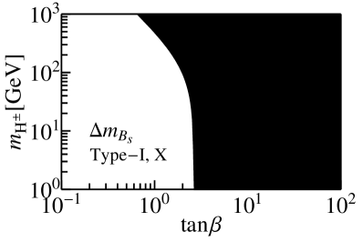
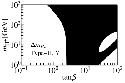
Figure 5: Constraints on the parameter space $(\tan\beta,m_{H^{\pm}})$ of the four types of 2HDM from $\Delta m_{B_{s}}$. The allowed regions are shown in black.

The mixing parameter $\Delta m_{B_{s}}$ is proportional to the Inami-Lim function $S(x_{t},x_{H^{\pm}})$. In the leading order (LO) approximation and taking $m_{H^{\pm}}=500\,\text{GeV}$, we have numerically

$$\frac{S(x_{t},x_{H^{\pm}})}{S_{\rm SM}(x_{t},x_{H^{\pm}})}=\begin{cases}\displaystyle 1+\frac{3.5\times 10^{-2}}{\tan^{4}\beta}+\frac{0.2}{\tan^{2}\beta},\hskip 2.84544pt&\text{type-I, X},\\ \displaystyle 1+\frac{3.5\times 10^{-2}}{\tan^{4}\beta}+\frac{0.2}{\tan^{2}\beta}+1.6\times 10^{-6}\tan^{2}\beta,\hskip 2.84544pt&\text{type-II, Y}.\end{cases}$$

From these results, we make the following observations:

• For the four different 2HDMs, the dominant effect is proportional to $\cot\beta$. They always work constructively with the SM contribution, even when the charged Higgs mass $m_{H^{\pm}}$ is not fixed but larger than about $90\,\rm GeV$.

• Since $\Delta m_{B_{s}}$ is only affected by charged Higgs, the contributions from type-I and -X (type-II and -Y) 2HDMs are the same. The type-I and -X Yukawa couplings of down-type quarks are different from the type-II and -Y ones. Thus, there is an additional term proportional to $\tan\beta$ in the latter two 2HDMs, however, suffering from down-type quark mass suppression.

In figure 5, the constraints on the parameter space $(\tan\beta,m_{H^{\pm}})$ from $\Delta m_{B_{s}}$ are shown. As expected, the allowed parameter space in type-I, -X 2HDMs and type-II, -Y 2HDMs are almost the same, in which the regions with small $\tan\beta$ are excluded. The difference appears in the region with large $\tan\beta$. However, the allowed charged Higgs mass in this region is below the LEP lower limit.

4.4 $\bar{B}\to X_{s}\gamma$ decay within 2HDM

The branching ratio of $\bar{B}\to X_{s}\gamma$ decay is proportional to $|C_{7\gamma}^{\text{eff}}(\mu_{b})|^{2}$ in the LO approximation. In 2HDM, the Wilson coefficient $C_{7\gamma}^{\text{eff}}(\mu_{b})$ reads numerically at $m_{H^{\pm}}=500\,\text{GeV}$ in the LO,

$$\frac{C_{7\gamma}^{\text{eff}}(\mu_{b})}{C_{7\gamma,\text{SM}}^{\text{eff}}(\mu_{b})}=\begin{cases}\displaystyle 1+\frac{0.02}{\tan^{2}\beta}-\frac{0.18}{\tan^{2}\beta},&\text{type-I, X},\\ \displaystyle 1+\frac{0.02}{\tan^{2}\beta}+0.18,&\text{type-II, Y}.\end{cases}$$

From these numerical results, we make the following observations:

• In the type-I and -X models, the 2HDM effect is proportional to $\cot\beta$ and destructive with the SM contribution.

• In the type-II and -Y models, the 2HDM contribution works constructively with the SM one. Besides the $\tan\beta$ terms, there are also $\beta$-independent terms, which dominate the 2HDM contribution for large $\tan\beta$.

• For the $\bar{B}\to X_{s}\gamma$, unlike the case of $B_{s}-\bar{B}_{s}$ mixing, the dominant operator $Q_{7\gamma}$ is a chirality-flipped operator with the chirality transition $b_{R}\to s_{L}$. Thus the contributions from down-type quark Yukawa couplings do not suffer mass suppression and dominate the ones from up-type quark Yukawa couplings.

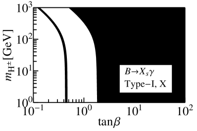
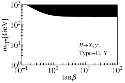
Figure 6: Constraints on the parameter space $(\tan\beta,m_{H^{\pm}})$ of the four types of 2HDM from ${\mathcal{B}}(\bar{B}\to X_{s}\gamma)$. The allowed regions are shown in black.

In figure 6, the constraints on the parameter space $(\tan\beta,m_{H^{\pm}})$ from $\mathcal{B}(\bar{B}\to X_{s}\gamma)$ are shown. The regions with small $\tan\beta$ are largely excluded in all the four types. However, there is still one solution in the type-I and -X 2HDMs, where the destructive interference between the SM and 2HDM contributions makes the coefficient $C_{7\gamma}^{\rm eff}$ sign-flipped. For the type-II and -Y 2HDMs, the charged Higgs mass is strongly bounded,

$$m_{H^{\pm}}\geq 259\,\text{GeV},$$

which mainly arises from the $\beta$-independent terms. This lower limit is stronger than the LEP bound.

4.5 $B\to\tau\nu$ decay within 2HDM

For $B\to\tau\nu$ decay, the numerical expressions of the branching ratio read,

$$\frac{\mathcal{B}(B\to\tau\nu)}{\mathcal{B}(B\to\tau\nu)_{\text{SM}}}=\begin{cases}\displaystyle(1-\frac{27.9}{m_{H^{\pm}}^{2}\tan^{2}\beta})^{2}=(1-\frac{1.1\times 10^{-4}}{\tan^{2}\beta})^{2},&\text{type-I},\\ \displaystyle(1-\frac{27.9\tan^{2}\beta}{m_{H^{\pm}}^{2}})^{2}=(1-1.1\times 10^{-4}{\tan^{2}\beta})^{2},&\text{type-II},\\ \displaystyle(1+\frac{27.9}{m_{H^{\pm}}^{2}})^{2}=(1+1.1\times 10^{-4})^{2},&\text{type-X, Y},\end{cases}$$

in which the second equality in each line holds for $m_{H^{\pm}}=500\,\text{GeV}$. Here, the 2HDM effects arise from tree-level charged Higgs with leptonic couplings, which make the following features:

• In all the four types, the 2HDM effects are largely suppressed by the charged Higgs mass.

• In the type-II (-I) model, the 2HDM effect is constructive with the SM one and proportional to $\tan\beta$ ($\cot\beta$). The large (small) $\tan\beta$ can compensate the mass suppression.

• In the type-X and -Y model, the 2HDM contribution is $\beta$-independent and proportional to $1/m_{H^{\pm}}$. Thus, small $m_{H^{\pm}}$ is expected to be strongly bounded.

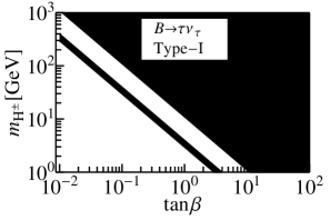
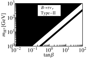
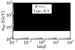
Figure 7: Constraints on the parameter space $(\tan\beta,m_{H^{\pm}})$ of the four types of 2HDM from $\mathcal{B}(B\to\tau\nu)$. The allowed regions are shown in black.

The constraints on the parameter space $(\tan\beta,m_{H^{\pm}})$ from ${\mathcal{B}}(B\to\tau\nu)$ are shown in figure 7. As expected, in the type-I (II) 2HDM, excluded regions mainly arise from the parameter space with small (large) $\tan\beta$. There also exists one solution (narrow band in figure 7), where the sign of the SM contribution is flipped by the 2HDMs. For the type-X and -Y 2HDMs, a $\beta$-independent bound on the charged Higgs mass is obtained, $m_{H^{\pm}}\geq 5\,\rm GeV$. However, this lower limit is much weaker than the LEP bound.

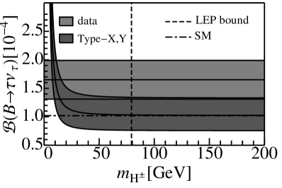
Figure 8: The type-X and -Y 2HDM predictions on $\mathcal{B}(B\to\tau\nu)$ with the theoretical uncertainty (dark shaded band) versus the experimental measurement (light shaded band).

Since $\mathcal{B}(B\to\tau\nu)$ is independent of $\tan\beta$ in type-X and type-Y, we also present its theoretical prediction as a function of $m_{H^{\pm}}$ in figure 8, which may be helpful for understanding these two models with reduced experimental and theoretical uncertainties in the future.

4.6 $B_{s,d}\to\mu^{+}\mu^{-}$ decays within 2HDM

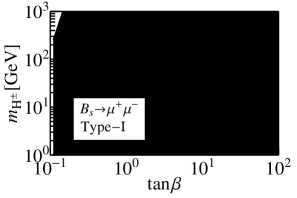
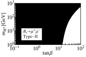
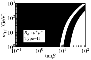
Figure 9: Constraints on the parameter space of the four types of 2HDM from $\overline{\mathcal{B}}(B_{s,d}\to\mu^{+}\mu^{-})$, plotted in the $\tan\beta-m_{H^{\pm}}$ plane. The allowed regions are shown in black.

For $B_{s}\to\mu^{+}\mu^{-}$ decay, taking $m_{H^{\pm}}=m_{H}=m_{A}=500\,\text{GeV}$, we get numerically

$$\frac{\overline{\mathcal{B}}(B_{s}\to\mu^{+}\mu^{-})}{\overline{\mathcal{B}}(B_{s}\to\mu^{+}\mu^{-})_{\rm SM}}=\begin{cases}\displaystyle 1-\frac{5.5\times 10^{-5}}{\tan^{2}\beta}+\frac{2.5\times 10^{-4}}{\tan^{4}\beta}+\frac{4.1\times 10^{-7}}{\tan^{6}\beta}+\frac{2.9\times 10^{-8}}{\tan^{8}\beta},&\text{type-I},\\ \displaystyle 1+3.4\times 10^{-6}-3.0\times 10^{-4}{\tan^{2}\beta}+{4.3\times 10^{-8}}{\tan^{4}\beta},&\text{type-II},\\ \displaystyle 1+5.5\times 10^{-5}-\frac{2.5\times 10^{-4}}{\tan^{2}\beta}+\frac{3.0\times 10^{-6}}{\tan^{4}\beta},&\text{type-X},\\ \displaystyle 1+3.1\times 10^{-4},&\text{type-Y}.\end{cases}$$

Here, both the charged and the neutral Higgs bosons are involved, which results in the following features:

• In all the four types, the 2HDM effects are strongly suppressed by the large mass of CP-even Higgs $m_{H}$ and small leptonic Yukawa coupling, and could be enhanced by the small mass of CP-odd Higgs $m_{A}$.

• In the type-II (-I and -X) models, the suppressed 2HDM contributions can be compensated by large $\tan\beta$ ($\cot\beta$).

• In the type-Y model, the 2HDM effect is $\beta$-independent. However, due to the large suppression, it can not provide strong bound on the masses of the Higgs bosons.

Under the constraints from $\overline{\mathcal{B}}(B_{s}\to\mu^{+}\mu^{-})$ and $\overline{\mathcal{B}}(B_{d}\to\mu^{+}\mu^{-})$, the allowed parameter space $(m_{H},m_{A},m_{H^{\pm}},\tan\beta)$ of the four types of 2HDM are obtained, which are plotted in the $\tan\beta-m_{H^{\pm}}$ plane in figure 9. Due to the large error bars, the current experimental data put almost no constraint on the model parameters, except for the small excluded regions in the type-I and -II 2HDMs.

4.7 Combined analysis and discrimination between the four 2HDMs

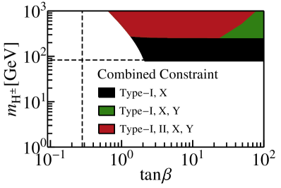
Figure 10: Combined constraints on the parameter space of the four types of 2HDM, plotted in the $\tan\beta-m_{H^{\pm}}$ plane. The horizontal dashed line denotes the direct bound on $m_{H^{\pm}}$ from the LEP experiment. The vertical dashed line denotes the bound on $\tan\beta$ from perturbative unitarity and vacuum stability.

Combining all the constraints mentioned in the previous sections, we obtain the surviving parameter space as shown in figure 10. From this plot, the following observations are made:

• For small $\tan\beta$, the most stringent constraints come from $\Delta m_{B_{s}}$ and $\mathcal{B}(\bar{B}\to X_{s}\gamma)$ in all the four types of 2HDM.

• For large $\tan\beta$, the flavour observables put almost no constraints in the type-I and -X models. The LEP bound on $m_{H^{\pm}}$ is still the most strongest. For type-II and -Y models, the constraints mainly come from $\mathcal{B}(\bar{B}\to X_{s}\gamma)$. The $B_{s,d}\to\mu^{+}\mu^{-}$ decays exclude one additional parameter space of the type-II 2HDM.

• When $m_{H^{\pm}}$ become large, the combined constraints from flavour observables are almost the same for all the four 2HDMs.

• The allowed region of the type-II model is contained in the one of the type-Y model, which stay in the survived parameter space of the type-I and -X 2HDMs. Therefore, the type-II model can be distinguished from the other 2HDMs in the green region in figure 10, and the type-II and -Y models from the other 2HDMs in the black region.

4.8 Other observables in $B_{s,d}\to\mu^{+}\mu^{-}$ within 2HDM

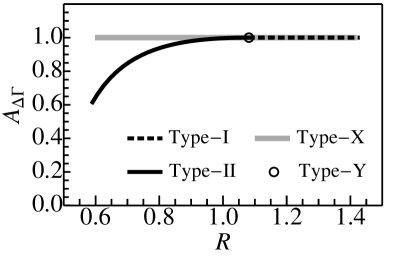
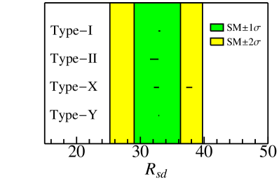
Figure 11: (a) Correlations in the $R-A_{\Delta\Gamma}$ plane and (b) predicted ranges of $R_{sd}$ in the four types of 2HDM.

At present, only the branching ratio of $B_{s,d}\to\mu^{+}\mu^{-}$ have been measured. For the observables $A_{\Delta\Gamma}$ and $R$ defined in eq. (3.15) and (3.16), we show in figure 11 the correlations between them within the four types of 2HDM, which are obtained in the parameter space given in section 4.7. The 2HDM predictions on $R_{sd}$ defined in eq. (3.17) are also shown in figure 11. From these plots, we make the following observations:

• For the type-II 2HDM, large derivations from the SM predictions for both $A_{\Delta\Gamma}$ and $R$ are allowed, since both the Wilson coefficients $C_{S}$ and $C_{P}$ can be significantly enhanced by large $\tan\beta$. It is also noted that the observable $R$ always decreases.

• For the type-I and -X 2HDMs, only large regions for $R$ are allowed. The reason is that the coefficient $C_{S}$ can not be enhanced by small $\tan\beta$, which has been excluded by the combined constraints discussed in section 4.7.

• For the type-Y 2HDM, as expected, its effects on both $A_{\Delta\Gamma}$ and $R$ are small.

• The observables $A_{\Delta\Gamma}$ and $R$ show the potential to discriminate the four types of 2HDM. For the type-I, -II and -X models, there always exists an allowed region for only one of them in the $R-A_{\Delta\Gamma}$ plane. Interestingly, the allowed region of the type-Y is located in the intersection of the regions of the other 2HDMs. With refined measurement of $A_{\Delta\Gamma}$ and $R$, one could distinguish one type 2HDM from others, or exclude all the four types.

• At present, due to large uncertainties, the observable $R_{sd}$ can not provide further information to distinguish between the four 2HDMs. It is also noted that $R_{sd}$ always decreases in the type-II 2HDM.

It is concluded that the observables $A_{\Delta\Gamma}$, $R$ and $R_{sd}$ in $B_{s,d}\to\mu^{+}\mu^{-}$ decays show high sensitivity to the Yukawa structure of the 2HDMs. Improved experimental measurements and theoretical predictions will make these observables more powerful to distinguish between the four types of 2HDM.

5 Conclusions

In this paper, we have studied the possibility to discriminate the four types of 2HDM in the light of recent flavour physics data, including the $B_{s}-\bar{B}_{s}$ mixing, the leptonic B-meson decays $B_{s,d}\to\mu^{+}\mu^{-}$ and $B\to\tau\nu$, and the inclusive radiative decay $\bar{B}\to X_{s}\gamma$, together with the experimental data from the direct search for Higgs bosons at LEP, Tevatron and LHC [85, 11, 12, 13, 14, 90] and the constraints from perturbative unitarity [100] and vacuum stability [99]. The outcomes of this combined analysis are summarized as follows:

• The flavour observables exhibit different dependence on the Yukawa couplings in the four types of 2HDMs. With the current experimental data, the allowed region of the type-II model is contained in the one of the type-Y model, which stay in the survived parameter space of the type-I and -X 2HDMs.

• The observables $A_{\Delta\Gamma}$ and $R$ in the $B_{s}\to\mu^{+}\mu^{-}$ decay, which arise from the sizable $B_{s}$ width difference, are investigated. The correlation between these two observables is found to be sensitive probe to the Yukawa structure of 2HDM.

With the experimental progress expected from the LHC and the future SuperKEKB, as well as the theoretical improvements, the constraints shown here are expected to be refined, which are helpful to discriminate the Yukawa structure if an extended Higgs sector is discovered in the future.

Acknoledgements

The work was supported by the National Natural Science Foundation of China (NSFC) under contract Nos. 11225523 and 11221504. X. D. Cheng was also supported by the CCNU-QLPL Innovation Fund (QLPL201308). X. B. Yuan was also supported by the CCNU-QLPL Innovation Fund (QLPL2011P01) and the Excellent Doctoral Dissertation Cultivation Grant from Central China Normal University.

Appendix A The Inami-Lim function $S(x_{t},x_{H^{\pm}})$

Within the four types of 2HDM discussed in section 2, the Inami-Lim function appearing in $B_{s}-\bar{B}_{s}$ mixing is given as [54]

$$S(x_{t},x_{H^{\pm}})=S_{WW}(x_{t})+2S_{WH}(x_{t},x_{H^{\pm}})+S_{HH}(x_{t},x_{H^{\pm}}),$$ (A.1)

where the basic functions $S_{WW}$ and $S_{WH,HH}$ correspond to the $W$ box and the Higgs box diagrams shown in figure 1, respectively. For convenience, their explicit expressions are given here:

$$S_{WW}(x_{t})$$

$$= +\left[1-\frac{11x_{t}}{4}+\frac{x_{t}^{2}}{4}-\frac{3x_{t}^{2}\ln x_{t}}{2(1-x_{t})}\right]\frac{x_{t}}{(1-x_{t})^{2}},$$ (A.2)

$$2S_{WH}(x_{t},x_{H^{\pm}})$$

$$= +\bigg{[}\frac{x_{t}^{2}x_{H^{\pm}}(x_{H^{\pm}}-4)}{2(1-x_{H^{\pm}})(x_{t}-x_{H^{\pm}})^{2}}\ln\frac{x_{t}}{x_{H^{\pm}}}+\frac{3x_{t}^{2}\ln x_{t}}{2{{(1-x_{t})}^{2}}(1-x_{H^{\pm}})}-\frac{x_{t}^{2}(4-x_{t})}{2(x_{H^{\pm}}-x_{t})(1-x_{t})}\bigg{]}(\xi_{A}^{u})^{2}$$

$$+\left[\frac{x_{t}^{2}}{(x_{H^{\pm}}-x_{t})^{2}}\right.\ln\frac{x_{H^{\pm}}}{x_{t}}+\left.\frac{x_{t}}{(x_{t}-x_{H^{\pm}})}\right]\times\left(\frac{1}{12}-\frac{m_{B_{s}}^{2}}{2\tilde{m}_{B_{s}}^{2}}\right)3\sqrt{x_{b}x_{s}}(\xi_{A}^{d})^{2},$$ (A.3)

$$4S_{HH}(x_{t},x_{H^{\pm}})$$

$$= +\left[\frac{x_{H^{\pm}}+x_{t}}{(x_{t}-x_{H^{\pm}})^{2}}+\frac{2x_{t}x_{H^{\pm}}}{(x_{H^{\pm}}-x_{t})^{3}}\ln\frac{x_{t}}{x_{H^{\pm}}}\right]x_{t}^{2}{(\xi_{A}^{u})^{4}}$$

$$+\left[\frac{x_{t}^{2}+x_{t}x_{H^{\pm}}}{(x_{H^{\pm}}-x_{t})^{2}x_{H^{\pm}}}+\frac{2x_{t}^{2}}{(x_{H^{\pm}}-x_{t})^{3}}\ln\frac{x_{t}}{x_{H^{\pm}}}\right]x_{b}x_{s}(\xi_{A}^{d})^{4}$$

$$+\left[\frac{2}{(x_{H^{\pm}}-x_{t})^{2}}+\frac{x_{t}+x_{H^{\pm}}}{(x_{H^{\pm}}-x_{t})^{3}}\ln\frac{x_{t}}{x_{H^{\pm}}}\right]\left(-\frac{3}{2}+\frac{m_{B_{s}}^{2}}{\tilde{m}_{B_{s}}^{2}}\right)x_{t}^{2}\sqrt{x_{b}x_{s}}(\xi_{A}^{u}\xi_{A}^{d})^{2}$$

$$+\left[\frac{2}{(x_{H^{\pm}}-x_{t})^{2}}+\frac{x_{t}+x_{H^{\pm}}}{(x_{H^{\pm}}-x_{t})^{3}}\right]\left[(x_{b}+x_{s})\frac{5m_{B_{s}}^{2}}{2\tilde{m}_{B_{s}}^{2}}+\sqrt{x_{b}x_{s}}\left(1-\frac{6m_{B_{s}}^{2}}{\tilde{m}_{B_{s}}^{2}}\right)\right]x_{t}^{2}(\xi_{A}^{u}\xi_{A}^{d})^{2},$$ (A.4)

with $\tilde{m}_{B_{s}}^{2}\equiv(\overline{m}_{b}(\overline{m}_{b})+\overline{m}_{s}(\overline{m}_{b}))^{2}$ and $x_{q}\equiv(\overline{m}_{q}(\overline{m}_{b}))^{2}/m_{W}^{2}$ for $q=s,b$.

Appendix B The Wilson coefficients $C_{S}$ and $C_{P}$

Within the four types of 2HDM discussed in section 2, the Wilson coefficients $C_{S}$ and $C_{P}$ appearing in the effective Hamiltonian of $B_{s,d}\to\mu^{+}\mu^{-}$ are given as [67]

$$C_{S} =C_{S}^{\rm box}+C_{S}^{\rm peng}+C_{S}^{\rm self},$$

$$C_{P} =C_{P}^{\rm box}+C_{P}^{\rm peng}+C_{P}^{\rm self},$$ (B.1)

where the functions $C_{S,P}^{\rm box}$, $C_{S,P}^{\rm peng}$ and $C_{S,P}^{\rm self}$ correspond to the box, penguin and self-energy diagrams associated with Higgs bosons in figure 4. Based on the results in ref. [67], their explicit expressions are given here:

$$C_{S,P}^{\rm box} =\frac{m_{\mu}}{2}\frac{\xi_{A}^{\ell}\xi_{A}^{d}}{m_{W}^{2}}B_{+}(x_{H^{\pm}},x_{t}),$$

$$C_{S}^{\rm peng} =\frac{m_{\mu}}{2}\left[\frac{\cos(\alpha-\beta)\xi_{h}^{\ell}\xi_{A}^{d}}{m_{h}^{2}}(1-x_{H^{\pm}}+x_{h})-\frac{\sin(\beta-\alpha)\xi_{H}^{\ell}\xi_{A}^{d}}{m_{H}^{2}}\left(1-x_{H^{\pm}}+x_{H}\right)\right]P_{+}(x_{H^{\pm}},x_{t})$$

$$C_{P}^{\rm peng} =\frac{m_{\mu}}{2}\frac{\xi_{A}^{\ell}\xi_{A}^{d}}{m_{A}^{2}}(1-x_{H^{\pm}}+x_{A})P_{+}(x_{H^{\pm}},x_{t}),$$

$$C_{S}^{\rm self} =\frac{m_{\mu}}{2}\xi_{A}^{u}\xi_{A}^{d}\left(\frac{\xi_{H}^{\ell}\xi_{H}^{d}}{m_{H}^{2}}+\frac{\xi_{h}^{\ell}\xi_{h}^{d}}{m_{h}^{2}}\right)(x_{H^{\pm}}-1)P_{+}(x_{H^{\pm}},x_{t}),$$

$$C_{P}^{\rm self} =\frac{m_{\mu}}{2}\xi_{A}^{u}\xi_{A}^{d}\left(\frac{\xi_{A}^{\ell}\xi_{A}^{d}}{m_{A}^{2}}\right)(x_{H^{\pm}}-1)P_{+}(x_{H^{\pm}},x_{t}),$$ (B.2)

with the functions

$$B_{+}(x,y) =\frac{y}{x-y}\left(\frac{\ln y}{y-1}-\frac{\ln x}{x-1}\right),$$

$$P_{+}(x,y) =\frac{y}{x-y}\left(\frac{x\ln x}{x-1}-\frac{y\ln y}{y-1}\right).$$ (B.3)

References

- [1] S. Weinberg, Phys. Rev. D 13, 974 (1976),
- [2] S. Weinberg, Phys. Rev. D 19, 1277 (1979).
- [3] E. Gildener, Phys. Rev. D 14, 1667 (1976).
- [4] L. Susskind, Phys. Rev. D 20, 2619 (1979).
- [5] G. ’t Hooft, C. Itzykson, A. Jaffe, H. Lehmann, P. K. Mitter, I. M. Singer and R. Stora, NATO Adv. Study Inst. Ser. B Phys. 59, pp.1 (1980).
- [6] T. Schwetz, M. A. Tortola and J. W. F. Valle, New J. Phys. 10, 113011 (2008) [arXiv:0808.2016 [hep-ph]].
- [7] A. D. Sakharov, Pisma Zh. Eksp. Teor. Fiz. 5, 32 (1967).
- [8] A. D. Sakharov, [JETP Lett. 5, 24 (1967)].
- [9] A. D. Sakharov, [Sov. Phys. Usp. 34, 392 (1991)].
- [10] A. D. Sakharov, [Usp. Fiz. Nauk 161, 61 (1991)].
- [11] G. Aad et al. [ATLAS Collaboration], Phys. Lett. B 716, 1 (2012) [arXiv:1207.7214 [hep-ex]].
- [12] G. Aad et al. [ATLAS Collaboration], Phys. Lett. B 726, 88 (2013) [arXiv:1307.1427 [hep-ex]].
- [13] S. Chatrchyan et al. [CMS Collaboration], Phys. Lett. B 716, 30 (2012) [arXiv:1207.7235 [hep-ex]].
- [14] S. Chatrchyan et al. [CMS Collaboration], JHEP 1306, 081 (2013) [arXiv:1303.4571 [hep-ex]].
- [15] P. W. Higgs, Phys. Rev. Lett. 13, 508 (1964).
- [16] P. W. Higgs, Phys. Lett. 12, 132 (1964).
- [17] P. W. Higgs, Phys. Rev. 145, 1156 (1966).
- [18] F. Englert and R. Brout, Phys. Rev. Lett. 13, 321 (1964).
- [19] G. S. Guralnik, C. R. Hagen and T. W. B. Kibble, Phys. Rev. Lett. 13, 585 (1964).
- [20] T. W. B. Kibble, Phys. Rev. 155, 1554 (1967).
- [21] A. Pilaftsis, Phys. Rev. D 58, 096010 (1998) [hep-ph/9803297].
- [22] G. C. Branco, P. M. Ferreira, L. Lavoura, M. N. Rebelo, M. Sher and J. P. Silva, Phys. Rept. 516, 1 (2012) [arXiv:1106.0034 [hep-ph]].
- [23] B. McWilliams and L. -F. Li, Nucl. Phys. B 179, 62 (1981).
- [24] O. U. Shanker, Nucl. Phys. B 206, 253 (1982).
- [25] W. -S. Hou, Phys. Lett. B 296, 179 (1992).
- [26] R. S. Chivukula and H. Georgi, Phys. Lett. B 188, 99 (1987).
- [27] A. J. Buras, P. Gambino, M. Gorbahn, S. Jager and L. Silvestrini, Phys. Lett. B 500, 161 (2001) [hep-ph/0007085].
- [28] G. D’Ambrosio, G. F. Giudice, G. Isidori and A. Strumia, Nucl. Phys. B 645, 155 (2002) [hep-ph/0207036].
- [29] A. V. Manohar and M. B. Wise, Phys. Rev. D 74, 035009 (2006) [hep-ph/0606172].
- [30] A. Pich and P. Tuzon, Phys. Rev. D 80, 091702 (2009) [arXiv:0908.1554 [hep-ph]].
- [31] S. L. Glashow and S. Weinberg, Phys. Rev. D 15, 1958 (1977).
- [32] M. Aoki, S. Kanemura, K. Tsumura and K. Yagyu, Phys. Rev. D 80, 015017 (2009) [arXiv:0902.4665 [hep-ph]].
- [33] S. D. Rindani, R. Santos and P. Sharma, JHEP 1311, 188 (2013) [arXiv:1307.1158].
- [34] V. D. Barger, J. L. Hewett and R. J. N. Phillips, Phys. Rev. D 41, 3421 (1990).
- [35] J. F. Gunion, H. E. Haber, G. L. Kane and S. Dawson, Front. Phys. 80, 1 (2000).
- [36] R. A. Diaz, hep-ph/0212237.
- [37] A. Djouadi, Phys. Rept. 459, 1 (2008) [hep-ph/0503173].
- [38] Z. -j. Xiao and L. -x. Lu, Phys. Rev. D 74, 034016 (2006) [hep-ph/0605076].
- [39] Q. Chang and Y. -D. Yang, Phys. Lett. B 676, 88 (2009) [arXiv:0808.2933 [hep-ph]].
- [40] F. Mahmoudi and O. Stal, Phys. Rev. D 81, 035016 (2010) [arXiv:0907.1791 [hep-ph]].
- [41] S. Kanemura, K. Tsumura and H. Yokoya, Phys. Rev. D 85, 095001 (2012) [arXiv:1111.6089 [hep-ph]], arXiv:1201.6489 [hep-ph].
- [42] K. Yagyu, arXiv:1204.0424 [hep-ph].
- [43] M. Jung, X. -Q. Li and A. Pich, JHEP 1210, 063 (2012) [arXiv:1208.1251 [hep-ph]].
- [44] T. Hermann, M. Misiak and M. Steinhauser, JHEP 1211, 036 (2012) [arXiv:1208.2788 [hep-ph]].
- [45] A. Celis, M. Jung, X. -Q. Li and A. Pich, JHEP 1301, 054 (2013) [arXiv:1210.8443 [hep-ph]].
- [46] C. -Y. Chen and S. Dawson, Phys. Rev. D 87, no. 5, 055016 (2013) [arXiv:1301.0309 [hep-ph]].
- [47] B. Grinstein and P. Uttayarat, JHEP 1306, 094 (2013) [Erratum-ibid. 1309, 110 (2013)] [arXiv:1304.0028 [hep-ph]].
- [48] O. Eberhardt, U. Nierste and M. Wiebusch, JHEP 1307, 118 (2013) [arXiv:1305.1649 [hep-ph]].
- [49] S. Kanemura, K. Tsumura and H. Yokoya, Phys. Rev. D 88, 055010 (2013) [arXiv:1305.5424 [hep-ph]].
- [50] V. Barger, L. L. Everett, H. E. Logan and G. Shaughnessy, arXiv:1307.3676 [hep-ph].
- [51] K. De Bruyn, R. Fleischer, R. Knegjens, P. Koppenburg, M. Merk, A. Pellegrino and N. Tuning, Phys. Rev. Lett. 109, 041801 (2012) [arXiv:1204.1737 [hep-ph]].
- [52] A. Lenz, U. Nierste, J. Charles, S. Descotes-Genon, A. Jantsch, C. Kaufhold, H. Lacker and S. Monteil et al., Phys. Rev. D 83, 036004 (2011) [arXiv:1008.1593 [hep-ph]].
- [53] A. Lenz, U. Nierste, J. Charles, S. Descotes-Genon, H. Lacker, S. Monteil, V. Niess and S. T’Jampens, Phys. Rev. D 86, 033008 (2012) [arXiv:1203.0238 [hep-ph]].
- [54] J. Urban, F. Krauss, U. Jentschura and G. Soff, Nucl. Phys. B 523, 40 (1998) [hep-ph/9710245].
- [55] X. -Q. Li, Y. -D. Yang and X. -B. Yuan, JHEP 1108, 075 (2011) [arXiv:1105.0364 [hep-ph]].
- [56] O. Deschamps, S. Descotes-Genon, S. Monteil, V. Niess, S. T’Jampens and V. Tisserand, Phys. Rev. D 82, 073012 (2010) [arXiv:0907.5135 [hep-ph]].
- [57] U. Haisch, “The inclusive radiative decay in the standard model,” Ph.D. Thesis.
- [58] A. J. Buras, arXiv:1102.5650 [hep-ph].
- [59] P. Gambino and M. Misiak, Nucl. Phys. B 611, 338 (2001) [hep-ph/0104034].
- [60] M. Ciuchini, G. Degrassi, P. Gambino and G. F. Giudice, Nucl. Phys. B 527, 21 (1998) [hep-ph/9710335].
- [61] M. Misiak, H. M. Asatrian, K. Bieri, M. Czakon, A. Czarnecki, T. Ewerth, A. Ferroglia and P. Gambino et al., Phys. Rev. Lett. 98, 022002 (2007) [hep-ph/0609232].
- [62] M. Misiak and M. Steinhauser, Nucl. Phys. B 683 (2004) 277 [hep-ph/0401041].
- [63] A. G. Akeroyd and C. H. Chen, Phys. Rev. D 75, 075004 (2007) [hep-ph/0701078].
- [64] A. G. Akeroyd, C. H. Chen and S. Recksiegel, Phys. Rev. D 77, 115018 (2008) [arXiv:0803.3517 [hep-ph]].
- [65] C. Bobeth, T. Ewerth, F. Kruger and J. Urban, Phys. Rev. D 64, 074014 (2001) [hep-ph/0104284].
- [66] A. J. Buras, J. Girrbach, D. Guadagnoli and G. Isidori, Eur. Phys. J. C 72, 2172 (2012) [arXiv:1208.0934 [hep-ph]].
- [67] H. E. Logan and U. Nierste, Nucl. Phys. B 586, 39 (2000) [hep-ph/0004139].
- [68] G. Buchalla and A. J. Buras, Nucl. Phys. B 400, 225 (1993).
- [69] M. Misiak and J. Urban, Phys. Lett. B 451, 161 (1999) [hep-ph/9901278].
- [70] G. Buchalla and A. J. Buras, Nucl. Phys. B 548, 309 (1999) [hep-ph/9901288].
- [71] C. Bobeth, M. Gorbahn and E. Stamou, Phys. Rev. D 89, 034023 (2014) [arXiv:1311.1348 [hep-ph]].
- [72] T. Hermann, M. Misiak and M. Steinhauser, JHEP 1312, 097 (2013) [arXiv:1311.1347 [hep-ph]].
- [73] C. Bobeth, M. Gorbahn, T. Hermann, M. Misiak, E. Stamou and M. Steinhauser, arXiv:1311.0903 [hep-ph].
- [74] RAaij et al. [LHCb Collaboration], Phys. Rev. D 87, 112010 (2013) [arXiv:1304.2600 [hep-ex]].
- [75] A. J. Buras, R. Fleischer, J. Girrbach and R. Knegjens, JHEP 1307, 77 (2013) [arXiv:1303.3820 [hep-ph]].
- [76] A. Bazavov et al. [Fermilab Lattice and MILC Collaborations], Phys. Rev. D 85, 114506 (2012) [arXiv:1112.3051 [hep-lat]].
- [77] H. Na, C. J. Monahan, C. T. H. Davies, R. Horgan, G. P. Lepage and J. Shigemitsu, Phys. Rev. D 86, 034506 (2012) [arXiv:1202.4914 [hep-lat]].
-
[78]
[UTfit Collaboration],
online update at:
http://www.utfit.org/UTfit/ResultsSummer2012PreICHEP - [79] J. Beringer et al. [Particle Data Group Collaboration], Phys. Rev. D 86, 010001 (2012).
-
[80]
J. Laiho, E. Lunghi and R. S. Van de Water,
Phys. Rev. D 81, 034503 (2010)
[arXiv:0910.2928 [hep-ph]].
Updates available on:
http://mypage.iu.edu/ elunghi/webpage/LatAves/page7/page7.html - [81] Y. Amhis et al. [Heavy Flavor Averaging Group Collaboration], arXiv:1207.1158 [hep-ex].
- [82] CMS and LHCb Collaborations [CMS and LHCb Collaboration], CMS-PAS-BPH-13-007.
- [83] R. Aaij et al. [LHCb Collaboration], Phys. Rev. Lett. 111, 101805 (2013) [arXiv:1307.5024 [hep-ex]].
- [84] S. Chatrchyan et al. [CMS Collaboration], Phys. Rev. Lett. 111, 101804 (2013) [arXiv:1307.5025 [hep-ex]].
- [85] A. Heister et al. [ALEPH Collaboration], Phys. Lett. B 543, 1 (2002) [hep-ex/0207054].
- [86] A. Abulencia et al. [CDF Collaboration], Phys. Rev. Lett. 96 (2006) 042003 [hep-ex/0510065].
- [87] V. M. Abazov et al. [D0 Collaboration], Phys. Lett. B 682 (2009) 278 [arXiv:0908.1811 [hep-ex]].
- [88] The ATLAS collaboration, ATLAS-CONF-2013-090.
- [89] S. Chatrchyan et al. [CMS Collaboration], JHEP 1207 (2012) 143 [arXiv:1205.5736 [hep-ex]].
- [90] T. Aaltonen et al. [CDF and D0 Collaborations], Phys. Rev. Lett. 109, 071804 (2012) [arXiv:1207.6436 [hep-ex]].
- [91] GG. Aad et al. [ATLAS Collaboration], Phys. Lett. B 726, 120 (2013) [arXiv:1307.1432 [hep-ex]].
- [92] S. Chatrchyan et al. [CMS Collaboration], Phys. Rev. Lett. 110, 081803 (2013) [arXiv:1212.6639 [hep-ex]].
- [93] [D0 Collaboration], DO-Note-6387-CONF.
- [94] A. Pich, EPJ Web Conf. 60, 02006 (2013) [arXiv:1307.7700].
- [95] D. Carmi, A. Falkowski, E. Kuflik, T. Volansky and J. Zupan, JHEP 1210, 196 (2012) [arXiv:1207.1718 [hep-ph]].
- [96] N. Craig, J. Galloway and S. Thomas, arXiv:1305.2424 [hep-ph].
- [97] S. Chang, S. K. Kang, J. -P. Lee, K. Y. Lee, S. C. Park and J. Song, JHEP 1305, 075 (2013) [arXiv:1210.3439 [hep-ph]].
- [98] S. Kanemura, T. Kasai and Y. Okada, Phys. Lett. B 471, 182 (1999) [hep-ph/9903289].
- [99] M. Sher, Phys. Rept. 179, 273 (1989).
- [100] B. W. Lee, C. Quigg and H. B. Thacker, Phys. Rev. D 16, 1519 (1977).