Hilfer–Prabhakar Derivatives and Some Applications

Abstract

We present a generalization of Hilfer derivatives in which Riemann–Liouville integrals are replaced by more general Prabhakar integrals. We analyze and discuss its properties. Furthermore, we show some applications of these generalized Hilfer–Prabhakar derivatives in classical equations of mathematical physics such as the heat and the free electron laser equations, and in difference-differential equations governing the dynamics of generalized renewal stochastic processes.

Keywords: Hilfer–Prabhakar derivatives, Prabhakar Integrals, Mittag–Leffler functions, Generalized Poisson Processes

1 Introduction

In the recent years fractional calculus has gained much interest mainly thanks to the increasing presence of research works in the applied sciences considering models based on fractional operators. Beside that, the mathematical study of fractional calculus has proceeded, leading to intersections with other mathematical fields such as probability and the study of stochastic processes.

In the literature, several different definitions of fractional integrals and derivatives are present. Some of them such as the Riemann–Liouville integral, the Caputo and the Riemann–Liouville derivatives are thoroughly studied and actually used in applied models. Other less-known definitions such as the Hadamard and Marchaud derivatives are mainly subject of mathematical investigation (the reader interested in fractional calculus in general can consult one of the classical reference texts such as [38, 20, 33]).

In this paper we introduce a novel generalization of derivatives of both Riemann–Liouville and Caputo types and show the effect of using it in equations of mathematical physics or related to probability. In order to do so, we start from the definition of generalized fractional derivatives given by R. Hilfer [16]. The so-called Hilfer fractional derivative is in fact a very convenient way to generalize both definitions of derivatives as it actually interpolates them by introducing only one additional real parameter $\nu\in[0,1]$. The further generalization that we are going to discuss in this paper is given by replacing Riemann–Liouville fractional integrals with Prabhakar integrals in the definition of Hilfer derivatives. We recall that the Prabhakar integral [36] is obtained by modifying the Riemann–Liouville integral operator by extending its kernel with a three-parameter Mittag–Leffler function, a function which extends the well-known two-parameter Mittag–Leffler function. This latter function was used by J.D. Tamarkin [44] in 1930 and later gained importance in treating problems of fractional relaxation and oscillation, see e.g. [25] for a grand survey. The Hilfer–Prabhakar derivative (which contains the Hilfer derivative as a specific case) interpolates the Prabhakar derivative, first introduced in [18] and its Caputo-like regularized counterpart. In Section 4, we study some of its properties and, in Section 5, we discuss some related applications of interest in mathematical physics and probability. We commence by analyzing the time-fractional heat equation involving Hilfer–Prabhakar derivatives. We discuss the main differences between the solution of the Cauchy problems involving the non-regularized and the regularized operators. Another integro-differential equation of interest for applications is the free electron laser (FEL) integral equation [6]. This equation arises in the description of the unsatured behavior of the free electron laser. Several generalizations of this equation involving other fractional operators have been studied in literature (see e.g. [19]). Taking inspiration from these works, we study a FEL-type integro-differential equation involving Hilfer–Prabhakar fractional derivatives. A further application that we study in Section 5.3 regards the derivation of a renewal point process which is in fact a direct generalization of the classical homogeneous Poisson process and the time-fractional Poisson process. The connection with Hilfer–Prabhakar derivatives comes from the fact that the state probabilities are governed by time-fractional difference-differential equations involving Hilfer–Prabhakar derivatives. We give a complete discussion of the main properties of this process, providing also the explicit form of the probability generating function, a subordination representation in terms of a time-changed Poisson process, and its renewal structure.

Before introducing the definition of the Hilfer–Prabhakar derivatives, in Section 2, in order to make the paper self-contained, we recall some basic definitions and results of fractional calculus. Section 3 presents instead the definition of Hilfer derivatives along with some of their properties.

2 Preliminaries on fractional calculus

Before introducing the non-regularized and regularized Hilfer–Prabhakar differential operators, for the reader’s convenience, in this section we recall some definitions of classical fractional operators. In particular, the classical Riemann–Liouville derivative and its regularized operator (the so-called Caputo derivative) will be described. However, in order to gain more insight on fractional calculus the reader can consult the classical reference books [38, 33, 20, 7].

Definition 2.1 (Riemann–Liouville integral).

Let $f\in L^{1}_{\text{loc}}[a,b]$, where $-\infty\leq a<t<b\leq\infty$, be a locally integrable real-valued function. The Riemann–Liouville integral is defined as

$$I^{\alpha}_{a^{+}}f(t) =\frac{1}{\Gamma(\alpha)}\int_{a}^{t}\frac{f(u)}{(t-u)^{1-\alpha}}du=(f\ast K_{\alpha})(t),\qquad\alpha>0,$$ (1)

where $K_{\alpha}(t)=t^{\alpha-1}/\Gamma(\alpha)$.

Definition 2.2 (Riemann–Liouville derivative).

Let $f\in L^{1}[a,b]$, $-\infty\leq a<t<b\leq\infty$, and $f\ast K_{m-\alpha}\in W^{m,1}[a,b]$, $m=\lceil\alpha\rceil$, $\alpha>0$, where $W^{m,1}[a,b]$ is the Sobolev space defined as

$$W^{m,1}[a,b]=\left\{f\in L^{1}[a,b]\colon\frac{d^{m}}{dt^{m}}f\in L^{1}[a,b]\right\}.$$ (2)

The Riemann–Liouville derivative of order $\alpha>0$ is defined as

$$D^{\alpha}_{a^{+}}f(t)=\frac{d^{m}}{dt^{m}}I_{a^{+}}^{m-\alpha}f(t)=\frac{1}{\Gamma(m-\alpha)}\frac{d^{m}}{dt^{m}}\int_{a}^{t}(t-s)^{m-1-\alpha}f(s)ds.$$ (3)

For $n\in\mathbb{N}$, we denote by $AC^{n}\left[a,b\right]$ the space of real-valued functions $f\left(t\right)$ which have continuous derivatives up to order $n-1$ on $\left[a,b\right]$ such that $f^{\left(n-1\right)}\left(t\right)$ belongs to the space of absolutely continuous functions $AC\left[a,b\right]:$

$$AC^{n}\left[a,b\right]=\left\{f:\left[a,b\right]\rightarrow\mathbb{R}\colon\frac{d^{n-1}}{dx^{n-1}}f\left(x\right)\in AC\left[a,b\right]\right\}.$$ (4)

Definition 2.3 (Caputo derivative).

Let $\alpha>0$, $m=\lceil\alpha\rceil$, and $f\in AC^{m}[a,b]$. The Caputo derivative of order $\alpha>0$ is defined as

$${}^{C}D^{\alpha}_{a^{+}}f(t)=I_{a^{+}}^{m-\alpha}\frac{d^{m}}{dt^{m}}f(t)=\frac{1}{\Gamma(m-\alpha)}\int_{a}^{t}(t-s)^{m-1-\alpha}\frac{d^{m}}{ds^{m}}f(s)\,ds.$$ (5)

In the space of the functions belonging to $AC^{m}[a,b]$ the following relation between Riemann–Liouville and Caputo derivatives holds [17].

Theorem 2.1.

For $f\in AC^{m}[a,b]$, $m=\lceil\alpha\rceil$, $\alpha\in\mathbb{R}^{+}\backslash\mathbb{N}$, the Riemann–Liouville derivative of order $\alpha$ of $f$ exists almost everywhere and it can be written as

$$D_{a^{+}}^{\alpha}f(t)={}^{C}D_{a^{+}}^{\alpha}f(t)+\sum_{k=0}^{m-1}\frac{(x-a)^{k-\alpha}}{\Gamma(k-\alpha+1)}f^{(k)}(a^{+}).$$ (6)

The above theorem gives the set of functions where the Riemann–Liouville derivative can be regularized. Moreover, if $f(t)\in AC^{m}[a,b]$, we have (see e.g. [1])

$$\lim_{t\to a^{+}}\frac{d^{k}}{dt^{k}}I_{a^{+}}^{m-\alpha}f(t)=0,\qquad\forall\quad 0\leq k\leq m-1.$$ (7)

Indeed, taking the Laplace transform of both sides of (6) the equality holds if (7) is true.

See also Gorenflo and Mainardi [11] for more information. In that paper (page 228) the Caputo fractional derivative was baptized so, ad late it gained rising popularity by Podlubny’s book [33] on fractional differential equations.

3 Hilfer derivatives

In a series of works (see [17] and the references therein), R. Hilfer studied applications of a generalized fractional operator having the Riemann–Liouville and the Caputo derivatives as specific cases (see also [45, 43]).

Definition 3.1 (Hilfer derivative).

Let $\mu\in(0,1)$, $\nu\in[0,1]$, $f\in L^{1}[a,b]$, $-\infty\leq a<t<b\leq\infty$, $f\ast K_{(1-\nu)(1-\mu)}\in AC^{1}[a,b]$. The Hilfer derivative is defined as

$$D^{\mu,\nu}_{a^{+}}f(t)=\left(I_{a^{+}}^{\nu(1-\mu)}\frac{d}{dt}(I_{a^{+}}^{(1-\nu)(1-\mu)}f)\right)(t),$$ (8)

Hereafter and without loss of generality we set $a=0$. The generalization (8), for $\nu=0$, coincides with the Riemann–Liouville derivative (3) and for $\nu=1$ with the Caputo derivative (5). A relevant point in the following discussion regards the initial conditions that should be considered in order to solve fractional Cauchy problems involving Hilfer derivatives. Indeed, in view of the Laplace transform of the Hilfer derivative ([45], formula (1.6))

$$\mathcal{L}[D^{\mu,\nu}_{0^{+}}f](s)=s^{\mu}\mathcal{L}[f](s)-s^{\nu(\mu-1)}(I^{(1-\nu)(1-\mu)}_{0^{+}}f)(0^{+}),$$ (9)

it is clear that the initial conditions that must be considered are of the form $(I_{0^{+}}^{(1-\nu)(1-\mu)}f)(0^{+})$, i.e. on the initial value of the fractional integral of order $(1-\nu)(1-\mu)$. These initial conditions do not have a clear physical meaning unless $\nu=1$. In order to obtain a regularized version of the Hilfer derivative, we must restrict ourselves to the set of absolutely continuous functions $AC^{1}[0,b]$ and therefore applying Theorem 2.1 we obtain, for $\mu\in(0,1)$,

$$D^{\mu,\nu}_{0^{+}}f(t) =\left(I_{0^{+}}^{\nu(1-\mu)}\frac{d}{dt}(I_{0^{+}}^{(1-\nu)(1-\mu)}f)\right)(t)$$ (10)

$$=\left(I_{0^{+}}^{\nu(1-\mu)}I_{0^{+}}^{(1-\nu)(1-\mu)}\frac{d}{dt}f\right)(t)+I_{0^{+}}^{\nu(1-\mu)}\frac{t^{\nu\mu-\nu-\mu}f(0^{+})}{\Gamma(1-\nu-\mu+\nu\mu)}$$

$$=I_{0^{+}}^{1-\mu}\frac{d}{dt}f(t)+\frac{t^{-\mu}f(0^{+})}{\Gamma(1-\mu)}={}^{C}D^{\mu}_{0^{+}}f(t)+\frac{t^{-\mu}f(0^{+})}{\Gamma(1-\mu)},$$

where we used the well-known semi-group property of Riemann–Liouville integrals and where ${}^{C}D^{\mu}_{0^{+}}$ is the Caputo derivative (5). From (10) it follows that in the space $AC^{1}[0,b]$ the Hilfer derivative (8) coincides with the Riemann–Liouville derivative of order $\mu$, and the regularized Hilfer derivative can be written as

$$D^{\mu,\nu}_{0^{+}}f(t)-\frac{t^{-\mu}f(0^{+})}{\Gamma(1-\mu)},$$ (11)

which coincides with ${}^{C}D^{\mu}_{0^{+}}$ and which in fact does not depend on the parameter $\nu$.

4 Hilfer–Prabhakar derivatives

We introduce a generalization of Hilfer derivatives by substituting in (8) the Riemann–Liouville integrals with a more general integral operator with kernel

$$e^{\gamma}_{\rho,\mu,\omega}(t)=t^{\mu-1}E^{\gamma}_{\rho,\mu}\left(\omega t^{\rho}\right),\qquad t\in\mathbb{R},\>\rho,\mu,\omega,\gamma\in\mathbb{C},\>\Re(\rho),\Re(\mu)>0,$$ (12)

where

$$E^{\gamma}_{\rho,\mu}(x)=\sum_{k=0}^{\infty}\frac{\Gamma(\gamma+k)}{\Gamma(\gamma)\Gamma(\rho k+\mu)}\frac{x^{k}}{k!},$$ (13)

is the generalized Mittag–Leffler function first investigated in [36]. The so-called Prabhakar integral is defined as follows [36, 18].

Definition 4.1 (Prabhakar integral).

Let $f\in L^{1}[0,b]$, $0<t<b\leq\infty$. The Prabhakar integral can be written as

$$\mathbf{E}^{\gamma}_{\rho,\mu,\omega,0^{+}}f(t)=\int_{0}^{t}(t-y)^{\mu-1}E^{\gamma}_{\rho,\mu}\left[\omega(t-y)^{\rho}\right]f(y)dy=(f\ast e^{\gamma}_{\rho,\mu,\omega})(t),$$ (14)

where $\rho,\mu,\omega,\gamma\in\mathbb{C}$, with $\Re(\rho),\Re(\mu)>0$.

We also recall that the left-inverse to the operator (14), the Prabhakar derivative, was introduced in [18]. We define it below in a slightly different form.

Definition 4.2 (Prabhakar derivative).

Let $f\in L^{1}[0,b]$, $0<x<b\leq\infty$, and $f\ast e_{\rho,m-\mu,\omega}^{-\gamma}(\cdot)\in W^{m,1}[0,b]$, $m=\lceil\mu\rceil$. The Prabhakar derivative is defined as

$$\mathbf{D}^{\gamma}_{\rho,\mu,\omega,0^{+}}f(x)=\frac{d^{m}}{dx^{m}}\mathbf{E}^{-\gamma}_{\rho,m-\mu,\omega,0^{+}}f(x)$$ (15)

where $\mu,\omega,\gamma,\rho\in\mathbb{C}$, $\Re(\mu),\Re(\rho)>0$.

Observing now that the Riemann–Liouville integrals in (3) can be expressed in terms of Prabhakar integrals as

$$I_{0^{+}}^{m-(\mu+\theta)}f(x)=\mathbf{E}^{0}_{\rho,m-(\mu+\theta),\omega,0^{+}}f(x),$$ (16)

we have that,

$$\mathbf{D}^{\gamma}_{\rho,\mu,\omega,0^{+}}f(x) =\frac{d^{m}}{dx^{m}}\mathbf{E}^{-\gamma}_{\rho,m-\mu,\omega,0^{+}}f(x)$$ (17)

$$=\frac{d^{m}}{dx^{m}}I^{m-(\mu+\theta)}\mathbf{E}^{-\gamma}_{\rho,\theta,\omega,0^{+}}f(x)$$

$$=D^{\mu+\theta}_{0^{+}}\mathbf{E}^{-\gamma}_{\rho,\theta,\omega,0^{+}}f(x),\qquad\theta\in\mathbb{C},\>\Re(\theta)>0,$$

where we used the fact that (see [18], Theorem 8)

$$\mathbf{E}_{\rho,\mu,\omega,0^{+}}^{\gamma}\mathbf{E}_{\rho,\nu,\omega,0^{+}}^{\sigma}f(x)=\mathbf{E}_{\rho,\mu+\nu,\omega,0^{+}}^{\gamma+\sigma}f(x).$$ (18)

Note that formula (17) concides with the definition given by [18]. As expected, the inverse operator (17) of the Prabhakar integral generalizes the Riemann–Liouville derivative. Its regularized Caputo counterpart is given, for functions $f\in AC^{m}[0,b]$, $0<x<b\leq\infty$, by

$${}^{C}\mathbf{D}^{\gamma}_{\rho,\mu,\omega,0^{+}}f(x) =\mathbf{E}^{-\gamma}_{\rho,m-\mu,\omega,0^{+}}\frac{d^{m}}{dx^{m}}f(x)$$ (19)

$$=\mathbf{D}^{\gamma}_{\rho,\mu,\omega,0^{+}}f(x)-\sum_{k=0}^{m-1}x^{k-\mu}E^{-\gamma}_{\rho,k-\mu+1}(\omega x^{\rho})f^{(k)}(0^{+}).$$

Proposition 4.1.

Let $\mu>0$ and $f\in AC^{m}[0,b]$, $0<x<b\leq\infty$. Then

$${}^{C}\mathbf{D}^{\gamma}_{\rho,\mu,\omega,0^{+}}f(x)=\mathbf{D}^{\gamma}_{\rho,\mu,\omega,0^{+}}\left[f(x)-\sum_{k=0}^{m-1}\frac{x^{k}}{k!}f^{(k)}(0^{+})\right].$$ (20)

Proof.

It easily follows from (17) and Corollary 2.3 of [18]. ∎

We are now ready to define the Hilfer–Prabhakar derivative, interpolating (19) and (17).

Definition 4.3 (Hilfer–Prabhakar derivative).

Let $\mu\in(0,1)$, $\nu\in[0,1]$, and let $f\in L^{1}[a,b]$, $0<t<b\leq\infty$, $f\ast e_{\rho,(1-\nu)(1-\mu),\omega}^{-\gamma(1-\nu)}(\cdot)\in AC^{1}[0,b]$. The Hilfer–Prabhakar derivative is defined by

$$\mathcal{D}^{\gamma,\mu,\nu}_{\rho,\omega,0^{+}}f(t)=\left(\mathbf{E}_{\rho,\nu(1-\mu),\omega,0^{+}}^{-\gamma\nu}\frac{d}{dt}(\mathbf{E}_{\rho,(1-\nu)(1-\mu),\omega,0^{+}}^{-\gamma(1-\nu)}f)\right)(t),$$ (21)

where $\gamma,\omega\in\mathbb{R}$, $\rho>0$, and where $\mathbf{E}_{\rho,0,\omega,0^{+}}^{0}f=f$.

We observe that (21) reduces to the Hilfer derivative for $\gamma=0$. Moreover, for $\nu=1$ and $\nu=0$ it coincides with (19) and (17), respectively (note that $m=1$).

Lemma 4.1.

The Laplace transform of (21) is given by

$$\mathcal{L}\left(\mathbf{E}_{\rho,\nu(1-\mu),\omega,0^{+}}^{-\gamma\nu}\frac{d}{dt}(\mathbf{E}_{\rho,(1-\nu)(1-\mu),\omega,0^{+}}^{-\gamma(1-\nu)}f)\right)(s)$$ (22)

$$=s^{\mu}[1-\omega s^{-\rho}]^{\gamma}\mathcal{L}[f](s)-s^{-\nu(1-\mu)}[1-\omega s^{-\rho}]^{\gamma\nu}\left[\mathbf{E}^{-\gamma(1-\nu)}_{\rho,(1-\nu)(1-\mu),\omega,0^{+}}f(t)\right]_{t=0^{+}}.$$

Proof.

By recurring to formula (2.19) of [18], i.e.

$$\mathcal{L}\left[t^{\mu-1}E^{-\gamma}_{\rho,\mu}(\omega t^{\rho})\right](s)=s^{-\mu}(1-\omega s^{-\rho})^{\gamma},\qquad\gamma,\omega,\rho,\mu\in\mathbb{C},\>\Re(\mu)>0,$$ (23)

with $s\in\mathbb{C}$, $\Re(s)>0$, $|\omega s^{-\rho}|<1$. We can write

$$\mathcal{L} \left(\mathbf{E}_{\rho,\nu(1-\mu),\omega,0^{+}}^{-\gamma\nu}\frac{d}{dt}(\mathbf{E}_{\rho,(1-\nu)(1-\mu),\omega,0^{+}}^{-\gamma(1-\nu)}f)\right)(s)$$ (24)

$$={} \mathcal{L}\left[t^{\nu(1-\mu)-1}E^{-\gamma\nu}_{\rho,\nu(1-\mu)}(\omega t^{\rho})\right](s)\cdot\mathcal{L}\left[\frac{d}{dt}(\mathbf{E}_{\rho,(1-\nu)(1-\mu),\omega,0^{+}}^{-\gamma(1-\nu)}f)\right](s)$$

$$={} s^{-\nu(1-\mu)}[1-\omega s^{-\rho}]^{\gamma\nu}s\,\mathcal{L}\left[t^{(1-\nu)(1-\mu)-1}E^{-\gamma(1-\nu)}_{\rho,(1-\nu)(1-\mu)}(\omega t^{\rho})\right](s)\>\mathcal{L}[f](s)$$

$$-s^{-\nu(1-\mu)}[1-\omega s^{-\rho}]^{\gamma\nu}\left[\mathbf{E}^{-\gamma(1-\nu)}_{\rho,(1-\nu)(1-\mu),\omega,0^{+}}f(t)\right]_{t=0^{+}}$$

$$={} s^{\mu}[1-\omega s^{-\rho}]^{\gamma}\mathcal{L}[f](s)-s^{-\nu(1-\mu)}[1-\omega s^{-\rho}]^{\gamma\nu}\left[\mathbf{E}^{-\gamma(1-\nu)}_{\rho,(1-\nu)(1-\mu),\omega,0^{+}}f(t)\right]_{t=0^{+}}.$$

∎

In order to consider Cauchy problems involving initial conditions depending only on the function and its integer-order derivatives we use the regularized version of (21), that is, for $f\in AC^{1}[0,b]$, we have

$${}^{C}\mathcal{D}^{\gamma,\mu}_{\rho,\omega,0^{+}}f(t)=\left(\mathbf{E}_{\rho,\nu(1-\mu),\omega,0^{+}}^{-\gamma\nu}\mathbf{E}_{\rho,(1-\nu)(1-\mu),\omega,0^{+}}^{-\gamma(1-\nu)}\frac{d}{dt}f\right)(t)=\left(\mathbf{E}_{\rho,1-\mu,\omega,0^{+}}^{-\gamma}\frac{d}{dt}f\right)(t),$$ (25)

We remark that, in the regularized version of the Hilfer–Prabhakar derivative (as well as in the regularized Hilfer derivative—see (10)), there is no dependence on the interpolating parameter $\nu$.

Lemma 4.2.

The Laplace transform of the operator (25) is given by

$$\mathcal{L}[{}^{C}\mathcal{D}^{\gamma,\mu}_{\rho,\omega,0^{+}}f](s)=s^{\mu}[1-\omega s^{-\rho}]^{\gamma}\mathcal{L}[f](s)-s^{\mu-1}[1-\omega s^{-\rho}]^{\gamma}f(0^{+}).$$ (26)

Proof.

It ensues from similar calculations to those in Lemma 4.1. ∎

From Lemmas 4.1 and 4.2 we have that the relation between the two operators (21) and (25) is given by

$${}^{C}\mathcal{D}^{\gamma,\mu}_{\rho,\omega,0^{+}}f(t)=\mathcal{D}^{\gamma,\mu,\nu}_{\rho,\omega,0^{+}}f(t)-t^{-\mu}E^{-\gamma}_{\rho,1-\mu}(\omega t^{\rho})f(0^{+}),$$ (27)

observing that, for absolutely continuous functions $f\in AC^{1}[0,b]$,

$$\left[\mathbf{E}^{-\gamma(1-\nu)}_{\rho,(1-\nu)(1-\mu),\omega,0^{+}}f(t)\right]_{t=0^{+}}=0,$$ (28)

and

$$\mathcal{L}^{-1}[s^{\mu-1}[1-\omega s^{-\rho}]^{\gamma}](t)\>f(0^{+})=t^{-\mu}E^{-\gamma}_{\rho,1-\mu}(\omega t^{\rho})\>f(0^{+}).$$ (29)

5 Applications

We show below some applications of Hilfer–Prabhakar derivatives in equations of interest for mathematical physics and probability.

5.1 Time-fractional heat equation

In the recent years more and more papers have been devoted to the mathematical analysis of versions of the time-fractional heat equation and to the study of its applications in mathematical physics and probability theory (see for example [29, 23, 24, 39, 46, 35] and the references therein).

Here we study a generalization of the time-fractional heat equation involving Hilfer–Prabhakar derivatives. We present analytical results for the time-fractional heat equation involving both regularized and non regularized Hilfer–Prabhakar derivatives in order to highlight the main differences between the two cases.

We start by considering the fractional heat equation involving the non-regularized operator $\mathcal{D}^{\gamma,\mu,\nu}_{\rho,\omega,0^{+}}$.

Theorem 5.1.

The solution to the Cauchy problem

$$\begin{cases}\mathcal{D}_{\rho,\omega,0^{+}}^{\gamma,\mu,\nu}u(x,t)=K\frac{\partial^{2}}{\partial x^{2}}u(x,t),&t>0,\>x\in\mathbb{R},\\ \left[\mathbf{E}_{\rho,(1-\nu)(1-\mu),\omega,0^{+}}^{-\gamma(1-\nu)}u(x,t)\right]_{t=0^{+}}=g(x),&\\ \lim_{x\rightarrow\pm\infty}u(x,t)=0,&\end{cases}$$ (30)

with $\mu\in(0,1)$, $\nu\in[0,1]$, $\omega\in\mathbb{R}$, $K,\rho>0$, $\gamma\geq 0$, is given by

$$u(x,t)=\int_{-\infty}^{+\infty}dk\,e^{-ikx}\hat{g}(k)\frac{1}{2\pi}\sum_{n=0}^{\infty}\left(-K\right)^{n}t^{\mu\left(n+1\right)-\nu(\mu-1)-1}E_{\rho,\mu\left(n+1\right)-\nu(\mu-1)}^{\gamma\left(n+1-\nu\right)}(\omega t^{\rho})k^{2n}.$$ (31)

Proof.

We denote with $\tilde{u}(x,s)=\mathcal{L}(u)(x,s)$ the Laplace transform with respect to the time variable $t$ and $\hat{u}(k,t)=\mathcal{F}(u)(k,t)$ the Fourier transform with respect to the space variable $x$. Taking the Fourier–Laplace transform of (30), by formula (22), we have

$$s^{\mu}(1-\omega s^{-\rho})^{\gamma}\hat{\tilde{u}}(k,s)-s^{\nu(\mu-1)}(1-\omega s^{-\rho})^{\gamma\nu}\hat{g}(k)=-Kk^{2}\hat{\tilde{u}}(k,s),$$ (32)

so that

$$\hat{\tilde{u}}(k,s) =\frac{s^{\nu(\mu-1)}(1-\omega s^{-\rho})^{\gamma\nu}\hat{g}(k)}{s^{\mu}(1-\omega s^{-\rho})^{\gamma}+Kk^{2}}$$ (33)

$$=s^{-\mu+\nu(\mu-1)}(1-\omega s^{-\rho})^{-\gamma(1-\nu)}\hat{g}(k)\left(1+\frac{Kk^{2}}{s^{\mu}(1-\omega s^{-\rho})^{\gamma}}\right)^{-1}$$

$$=\sum_{n=0}^{\infty}\left(-Kk^{2}\right)^{n}s^{-\mu\left(n+1\right)+\nu(\mu-1)}(1-\omega s^{-\rho})^{-\gamma\left(n+1-\nu\right)}\hat{g}(k),\qquad\left|\frac{Kk^{2}}{s^{\mu}(1-\omega s^{-\rho})^{\gamma}}\right|<1.$$

Inverting first the Laplace transform it yields

$$\hat{u}(k,t)=\sum_{n=0}^{\infty}\left(-K\right)^{n}t^{\mu\left(n+1\right)-\nu(\mu-1)-1}E_{\rho,\mu\left(n+1\right)-\nu(\mu-1)}^{\gamma\left(n+1-\nu\right)}(\omega t^{\rho})k^{2n}\hat{g}(k).$$ (34)

Note that the inversion term by term of the Laplace transform is possible in view of Theorem 30.1 by Doetsch [8] provided to choose a sufficiently large abscissa for the inverse integral and by recalling that the generalized Mittag Leffler function is defined as an absolutely convergent series. The convergence of (34) and in general of series of the same form (see below) can be proved by using the same technique as in Appendix C of [40]. Indeed the function (34) is in fact a repeated series:

$$\hat{u}(k,t)=\hat{g}(k)t^{-\nu(\mu-1)-1+\mu}\sum_{n=0}^{\infty}\frac{\left(-Kk^{2}\right)^{n}t^{\mu n}}{\Gamma(\gamma(n+1-\nu))}\sum_{r=0}^{\infty}\frac{(\omega t^{\rho})^{r}\Gamma(r+\gamma(n+1-\nu))}{r!\Gamma(\rho r+\mu(n+1)-\nu(\mu-1))}.$$ (35)

Since the three-parameter generalized Mittag–Leffler is an entire function, in order to prove the absolute convergence of (34) it is sufficient to show that for each $r\in\mathbb{N}\cup\{0\}$

$$\sum_{n=0}^{\infty}\frac{(-Kk^{2}t^{\mu})^{n}\Gamma(r+\gamma(n+1-\nu))}{\Gamma(\gamma(n+1-\nu))\Gamma(\rho r+\mu(n+1)-\nu(\mu-1))}$$ (36)

converges absolutely. We need to study the ratio

$$\left|\frac{(-Kk^{2}t^{\mu})^{n+1}\Gamma(r+\gamma(n+2-\nu))}{\Gamma(\gamma(n+2-\nu))\Gamma(\rho r+\mu(n+2)-\nu(\mu-1))}\frac{\Gamma(\gamma(n+1-\nu))\Gamma(\rho r+\mu(n+1)-\nu(\mu-1))}{(-Kk^{2}t^{\mu})^{n}\Gamma(r+\gamma(n+1-\nu))}\right|$$ (37)

$$=\left|(-Kk^{2}t^{\mu})\right|\left|\frac{\Gamma(\gamma(n+1-\nu)+\gamma+r)}{\Gamma(\gamma(n+1-\nu)+\gamma)}\right|\left|\frac{\Gamma(\gamma(n+1-\nu))}{\Gamma(\gamma(n+1-\nu)+r)}\right|\left|\frac{\Gamma(\rho r+\mu(n+1)-\nu(\mu-1))}{\Gamma(\rho r+\mu(n+1)-\nu(\mu-1)+\mu)}\right|$$

$$\approx\left|(-Kk^{2}t^{\mu})\right|\left[\rho r+\mu(n+1)-\nu(\mu-1)\right]^{-\mu}.$$

Last step of the above formula is valid for large values of $k$ and can be determined by means of the well-known asymptotics

$$\frac{\Gamma(z+a)}{\Gamma(z+b)}=z^{a-b}\left[1+\frac{(a-b)(a+b-1)}{2z}+O(z^{-2})\right],$$ (38)

for $|z|\to\infty$, $|\arg(z)|\leq\pi-\varepsilon$, $|\arg(z+a)|\leq\pi-\varepsilon$, $0<\varepsilon<\pi$. Formula (37) is zero for $n\to\infty$ implying absolute convergence of (36) and therefore of (34).

To conclude the proof of the theorem, by applying the inverse Fourier transform to (34) we obtain the claimed result. ∎

We now discuss the case with the regularized Hilfer–Prabhakar derivative ${}^{C}\mathcal{D}^{\gamma,\mu}_{\rho,\omega,0^{+}}$.

Theorem 5.2.

The solution to the Cauchy problem

$$\begin{cases}{}^{C}\mathcal{D}_{\rho,\omega,0^{+}}^{\gamma,\mu}u(x,t)=K\frac{\partial^{2}}{\partial x^{2}}u(x,t),&t>0,\>x\in\mathbb{R},\\ u(x,0^{+})=g(x),&\\ \lim_{x\rightarrow\pm\infty}u(x,t)=0,&\end{cases}$$ (39)

with $\mu\in(0,1)$, $\omega\in\mathbb{R}$, $K,\rho>0$, $\gamma\geq 0$, is given by

$$u(x,t)=\int_{-\infty}^{+\infty}dk\,e^{-ikx}\hat{g}(k)\frac{1}{2\pi}\sum_{n=0}^{\infty}\left(-Kt^{\mu}\right)^{n}E_{\rho,\mu n+1}^{\gamma n}\left(\omega t^{\rho}\right)k^{2n}.$$ (40)

Proof.

Taking the Fourier–Laplace transform of (39), by formula (26), we have that

$$s^{\mu}(1-\omega s^{-\rho})^{\gamma}\hat{\tilde{u}}(k,s)-s^{\mu-1}(1-\omega s^{-\rho})^{\gamma}\hat{g}(k)=-Kk^{2}\hat{\tilde{u}}(k,s),$$ (41)

so that

$$\hat{\tilde{u}}(k,s) =\frac{s^{\mu-1}(1-\omega s^{-\rho})^{\gamma}\hat{g}(k)}{s^{\mu}(1-\omega s^{-\rho})^{\gamma}+Kk^{2}}=s^{-1}\hat{g}(k)\left(1+\frac{Kk^{2}}{s^{\mu}(1-\omega s^{-\rho})^{\gamma}}\right)^{-1}$$ (42)

$$=\sum_{n=0}^{\infty}\left(-Kk^{2}\right)^{n}s^{-\mu n-1}(1-\omega s^{-\rho})^{-\gamma n}\hat{g}(k),\qquad\left|\frac{Kk^{2}}{s^{\mu}(1-\omega s^{-\rho})^{\gamma}}\right|<1.$$

Inverting first the Laplace transform (see the proof of Theorem 5.1 for more information on the inversion) it yields

$$\hat{u}(k,t)=\sum_{n=0}^{\infty}\left(-Kt^{\mu}\right)^{n}E_{\rho,\mu n+1}^{\gamma n}(\omega t^{\rho})k^{2n}\hat{g}(k).$$ (43)

By applying the inverse Fourier transform we obtain the claimed result. ∎

5.2 Fractional free electron laser equation

The free electron laser integro-differential equation

$$\begin{cases}\frac{dy}{dx}=-i\pi g\int_{0}^{x}(x-t)e^{i\eta(x-t)}y(t)dt,\qquad g,\eta\in\mathbb{R},\>x\in(0,1],\\ y(0)=1,\end{cases}$$ (44)

describes the unsaturated behavior of the free electron laser (FEL) (see for example [6]). In recent years many attempts to solve the generalized fractional integro-differential FEL equation have been proposed (see for example [19]). Here we consider the following fractional generalization of the FEL equation, involving Hilfer–Prabhakar derivatives.

$$\begin{cases}\mathcal{D}^{\gamma,\mu,\nu}_{\rho,\omega,0^{+}}y(x)=\lambda\mathbf{E}^{\varpi}_{\rho,\mu,\omega,0^{+}}y(x)+f(x),&x\in(0,\infty),\>f(x)\in L^{1}[0,\infty),\\ \left[\mathbf{E}^{-\gamma(1-\nu)}_{\rho,(1-\nu)(1-\mu),\omega,0^{+}}y(x)\right]_{x=0^{+}}=\kappa,&\kappa\geq 0,\end{cases}$$ (45)

where $\mu\in(0,1)$, $\nu\in[0,1]$, $\omega,\lambda\in\mathbb{C}$, $\rho>0$, $\gamma,\varpi\geq 0$. This generalizes the problem studied in [19], corresponding to $\nu=\gamma=0$. Here $f(x)$ is a given function. The original FEL equation is then retrieved for $\gamma=0$, $\nu=0$, $\mu\to 1$, $f\equiv 0$, $\lambda=-i\pi g$, $\omega=i\eta$, $\rho=\varpi=\kappa=1$.

We have the following

Theorem 5.3.

The solution to the Cauchy problem (45) is given by

$$y(x)=\kappa\sum_{k=0}^{\infty}\lambda^{k}x^{\nu(1-\mu)+\mu+2\mu k-1}E_{\rho,\nu(1-\mu)+\mu+2k\mu}^{\gamma+k(\varpi+\gamma)-\gamma\nu}(\omega x^{\rho})+\sum_{k=0}^{\infty}\lambda^{k}\mathbf{E}_{\rho,\mu(2k+1),\omega,0^{+}}^{\gamma+k(\varpi+\gamma)}f(x).$$ (46)

Proof.

By taking the Laplace transform of (45) (see (22)) we get

$$s^{\mu}(1-\omega s^{-\rho})^{\gamma}\mathcal{L}[y](s)-\kappa s^{-\nu(1-\mu)}(1-\omega s^{-\rho})^{\gamma\nu}=\lambda\mathcal{L}[x^{\mu-1}E_{\rho,\mu}^{\varpi}(\omega x^{\rho})](s)\cdot\mathcal{L}[y](s)+\mathcal{L}[f](s),$$ (47)

so that

$$\mathcal{L}[y](s)={} \frac{\kappa s^{-\nu(1-\mu)-\mu}(1-\omega s^{-\rho})^{\gamma\nu-\gamma}}{1-\lambda s^{-2\mu}(1-\omega s^{-\rho})^{-\varpi-\gamma}}+\frac{s^{-\mu}(1-\omega s^{-\rho})^{-\gamma}\mathcal{L}[f](s)}{1-\lambda s^{-2\mu}(1-\omega s^{-\rho})^{-\varpi-\gamma}}$$ (48)

$$={} \kappa\sum_{k=0}^{\infty}\lambda^{k}s^{-\nu(1-\mu)-\mu-2\mu k}(1-\omega s^{-\rho})^{\gamma\nu-\gamma-k(\varpi+\gamma)}$$

$$+\sum_{k=0}^{\infty}\lambda^{k}s^{-\mu(2k+1)}(1-\omega s^{-\rho})^{-\gamma-k(\varpi+\gamma)}\mathcal{L}[f](s).$$

Last step is valid for $|\lambda s^{-2\mu}(1-\omega s^{-\rho})^{-\varpi-\gamma}|$. Inverting the Laplace transform (see the proof of Theorem 5.1 for more information) and using the convolution theorem, we obtain the claimed result. ∎

Example 5.1.

Let us consider the Cauchy problem (45) with $\kappa=0$, $f(x)=x^{\mathfrak{m}-1}$. By direct calculation we have that

$$\mathbf{E}_{\rho,\mu(2k+1),\omega,0^{+}}^{\gamma+k(\varpi+\gamma)}x^{\mathfrak{m}-1}=\Gamma(\mathfrak{m})x^{\mu(2k+1)+\mathfrak{m}-1}E_{\rho,\mu(2k+1)+\mathfrak{m}}^{\gamma+k(\varpi+\gamma)}(\omega x^{\rho}),$$ (49)

and the explicit solution of the Cauchy problem is given by

$$y(x)=\Gamma(\mathfrak{m})x^{\mu+\mathfrak{m}-1}\sum_{k=0}^{\infty}(\lambda x^{2\mu})^{k}E_{\rho,\mu(2k+1)+\mathfrak{m}}^{\gamma+k(\varpi+\gamma)}(\omega x^{\rho}).$$ (50)

Example 5.2.

Let us consider the Cauchy problem (45) with $\kappa=0$, $f(x)=x^{\mathfrak{m}-1}E_{\rho,\mathfrak{m}}^{\sigma}(\omega x^{\rho})$. Recalling that

$$\mathbf{E}_{\rho,\mu(2k+1),\omega,0^{+}}^{\gamma+k(\varpi+\gamma)}x^{\mathfrak{m}-1}E_{\rho,\mathfrak{m}}^{\sigma}(\omega x^{\rho})=x^{\mu(2k+1)+\mathfrak{m}-1}E_{\rho,\mu(2k+1)+\mathfrak{m}}^{\gamma+k(\varpi+\gamma)+\sigma}(\omega x^{\rho}),$$ (51)

we obtain

$$y(x)=x^{\mu+\mathfrak{m}-1}\sum_{k=0}^{\infty}(\lambda x^{2\mu})^{k}E_{\rho,\mu(2k+1)+\mathfrak{m}}^{\gamma+k(\varpi+\gamma)+\sigma}(\omega x^{\rho}).$$ (52)

5.3 Fractional Poisson processes involving Hilfer–Prabhakar derivatives

In this section we present a generalization of the homogeneous Poisson process for which the governing difference-differential equations contain the regularized Hilfer–Prabhakar differential operator acting in time. The considered framework generalizes also the time-fractional Poisson process which in the recent years has become subject of intense research. It is well known that the state probabilities of the classical Poisson process and its time-fractional generalization can be found by solving an infinite system of difference-differential equations. We solve an analogous infinite system and find the corresponding state probabilities that we give in form of an infinite series and in integral form. As the zero state probability of a renewal process coincides with the residual time probability, we can characterize our process also by its waiting distribution (the common way of characterizing a renewal process). We will see in the following that the state probabilities of the generalized Poisson process are expressed by functions which in fact generalize the classical Mittag–Leffler function. The Mittag–Leffler function appeared as residual waiting time between events in renewal processes already in the Sixties of the past century, namely processes with properly scaled thinning out the sequence of events in a power law renewal process (see [10] and [27]). Such a process in essence is a fractional Poisson process. It must however be said that Gnedenko and Kovalenko did their analysis only in the Laplace domain, not recognizing their result as the Laplace transform of a Mittag–Leffler type function. Balakrishnan in 1985 [2] also found this Laplace transform as highly relevant for analysis of time-fractional diffusion processes, but did not identify it as arising from a Mittag–Leffler type function. In the Nineties of the past century the Mittag–Leffler function arrived at its deserved honour, more and more researchers became aware of it and used it. Let us only sketch a few highlights. Hilfer and Anton [15] were the first authors who explicitly introduced the Mittag–Leffler waiting-time density

$$f_{\mu}(t)=-\frac{d}{dt}E_{\mu}(-t^{\mu})=t^{\mu-1}E_{\mu,\mu}(-t^{\mu})$$ (53)

(writing it in form of a Mittag–Leffler function with two indices) into the theory of continuous time random walk. They showed that it is needed if one wants to get as evolution equation for the sojourn density the fractional variant of the Kolmogorov–Feller equation. In modern terminology they subordinated a random walk to the fractional Poisson process. By completely different argumentation the authors of [26] also discussed the relevance of $f_{\mu}(t)$ in theory of continuous time random walk. However, all these authors did not treat the fractional Poisson process as a subject of study in its own right but simply as useful for general analysis of certain stochastic processes. The detailed analytic and probabilistic investigation was started (as far as we know) in 2000 by Repin and Saichev [37]. More and more researchers then, often independently of each other, investigated this renewal process. Let us here only recall the few relevant papers [12, 13, 42, 4, 3, 5, 22, 31, 34, 30] and see also the references cited therein.

Let us thus start with the governing equations for the state probabilities. In view of Section 4 we define the following Cauchy problem involving the regularized operator ${}^{C}\mathcal{D}^{\gamma,\mu}_{\rho,\omega,0^{+}}$.

Definition 5.1 (Cauchy problem for the generalized fractional Poisson process).

$$\begin{cases}{}^{C}\mathcal{D}^{\gamma,\mu}_{\rho,-\phi,0^{+}}p_{k}(t)=-\lambda p_{k}(t)+\lambda p_{k-1}(t),&k\geq 0,\>t>0,\>\lambda>0,\\ p_{k}(0)=\begin{cases}1,\quad k=0,\\ 0,\quad k\geq 1,\end{cases}&\end{cases}$$ (54)

where $\phi>0$, $\gamma\geq 0$, $0<\rho\leq 1$, $0<\mu\leq 1$. We also have $0<\mu\lceil\gamma\rceil/\gamma-r\rho<1$, $\forall\>r=0,\dots,\lceil\gamma\rceil$, if $\gamma\neq 0$.

These ranges for the parameters are needed to ensure non-negativity of the solution (see Section 5.3.2 for more details). Multiplying both the terms of (54) by $v^{k}$ and adding over all $k$, we obtain the fractional Cauchy problem for the probability generating function $G(v,t)=\sum_{k=0}^{\infty}v^{k}p_{k}(t)$ of the counting number $N(t)$, $t\geq 0$,

$$\begin{cases}{}^{C}\mathcal{D}^{\gamma,\mu}_{\rho,-\phi,0^{+}}G(v,t)=-\lambda(1-v)G(v,t),&|v|\leq 1,\\ G(v,0)=1.&\end{cases}$$ (55)

Theorem 5.4.

The solution to (55) reads

$$G(v,t)=\sum_{k=0}^{\infty}(-\lambda t^{\mu})^{k}(1-v)^{k}E_{\rho,\mu k+1}^{\gamma k}(-\phi t^{\rho}),\qquad|v|\leq 1.$$ (56)

Proof.

In view of Lemma 4.2, we have

$$s^{\mu}[1+\phi s^{-\rho}]^{\gamma}\mathcal{L}[G](v,s)-s^{\mu-1}[1+\phi s^{-\rho}]^{\gamma}=-\lambda(1-v)\mathcal{L}[G](v,s),$$ (57)

so that

$$\mathcal{L}[G](v,s) =\frac{s^{\mu-1}[1+\phi s^{-\rho}]^{\gamma}}{s^{\mu}[1+\phi s^{-\rho}]^{\gamma}+\lambda(1-v)}=\frac{1}{s}\left(1+\frac{\lambda(1-v)}{s^{\mu}[1+\phi s^{-\rho}]^{\gamma}}\right)^{-1}$$ (58)

$$=\frac{1}{s}\sum_{k=0}^{\infty}\left[-\frac{\lambda(1-v)}{s^{\mu}[1+\phi s^{-\rho}]^{\gamma}}\right]^{k}=\sum_{k=0}^{\infty}(-\lambda(1-v))^{k}s^{-\mu k-1}[1+\phi s^{-\rho}]^{-k\gamma},$$

where $|\lambda(1-v)/[s^{\mu}(1+\phi s^{-\rho})^{\gamma}]|<1$. By using (23) we can invert the Laplace transform (58) obtaining the claimed result (for more details on the inversion and on the convergence of series of similar form of (56) the reader can consult the proof of Theorem 5.1). ∎

Remark 5.1.

Observe that for $\gamma=0$, we retrieve the classical result obtained for example in [21], formula (23). Indeed, from the fact that

$$E_{\rho,\mu k+1}^{0}(-\phi t^{\rho})=\sum_{r=0}^{\infty}\frac{(-\phi t^{\rho})^{r}\Gamma(r)}{r!\Gamma(\rho r+\mu k+1)\Gamma(0)}=\frac{1}{\Gamma(\mu k+1)},$$ (59)

(note that in the series representation of the three-parameter Mittag–Leffler function (59) each term is zero except that for $r=0$) equation (56) becomes

$$G(v,t)=\sum_{k=0}^{\infty}\frac{(-\lambda t^{\mu})^{k}(1-v)^{k}}{\Gamma(\mu k+1)}=E^{1}_{\mu,1}(-\lambda(1-v)t^{\mu}),$$ (60)

that coincides with equation (23) in [21].

From the probability generating function (56), we are now able to find the probability distribution at fixed time $t$ of $N(t)$, $t\geq 0$, governed by (54). Indeed, a simple binomial expansion leads to

$$G(v,t)=\sum_{k=0}^{\infty}v^{k}\sum_{r=k}^{\infty}(-1)^{r-k}\binom{r}{k}(\lambda t^{\mu})^{r}E_{\rho,\mu r+1}^{\gamma r}(-\phi t^{\rho}).$$ (61)

Therefore,

$$p_{k}(t)=\sum_{r=k}^{\infty}(-1)^{r-k}\binom{r}{k}(\lambda t^{\mu})^{r}E_{\rho,\mu r+1}^{\gamma r}(-\phi t^{\rho}),\qquad k\geq 0,\>t\geq 0.$$ (62)

We observe that, for $\gamma=0$,

$$p_{k}(t) =\sum_{r=k}^{\infty}(-1)^{r-k}\binom{r}{k}\frac{(\lambda t^{\mu})^{r}}{\Gamma(\mu r+1)}=(\lambda t^{\mu})^{k}E_{\mu,\mu k+1}^{k+1}(-\lambda t^{\mu})$$ (63)

$$=\frac{(\lambda t^{\mu})^{k}}{k!}E^{(k)}_{\mu,1}(-\lambda t^{\mu}),\qquad k\geq 0,\>t\geq 0,$$

The first expression of (63) coincides with equation (1.4) in [4]. The third one is a convenient representation involving the $k$th derivative of the two-parameter Mittag–Leffler function evaluated at $-\lambda t^{\mu}$. It is immediate to note, from (56), by inserting $v=1$, that $\sum_{k=0}^{\infty}p_{k}(t)=1$. From the generating function (56) much information on the behavior of the process can be extracted. From (54), with standard methods we can evaluate the mean value of $N(t)$. In order to do so, it suffices to differentiate equation (55) with respect to $v$ and to take $v=1$. We obtain

$$\begin{cases}{}^{C}\mathcal{D}^{\gamma,\mu}_{\rho,-\phi,0^{+}}\mathbb{E}N(t)=\lambda,&t>0,\\ \mathbb{E}N(t)\big{|}_{t=0}=0,&\end{cases}$$ (64)

whose solution is simply given by

$$\mathbb{E}N(t)=\lambda t^{\mu}E^{\gamma}_{\rho,1+\mu}(-\phi t^{\rho}),\qquad t\geq 0.$$ (65)

5.3.1 Subordination representation

In order to derive an alternative representation for the fractional Poisson process $N(t)$, $t\geq 0$, we present first some preliminaries. Consider the Cauchy problem

$$\begin{cases}{}^{C}\mathcal{D}^{\gamma,\mu}_{\rho,-\phi,0^{+}}h(x,t)=-\frac{\partial}{\partial x}h(x,t),&t>0,\>x\geq 0,\\ h(x,0^{+})=\delta(x).&\end{cases}$$ (66)

Representation (19) and the results obtained in [9] simply imply that the Laplace–Laplace transform of $h(x,t)$ can be written as

$$\tilde{\tilde{h}}(z,s)=\frac{s^{\mu-1}(1+\phi s^{-\rho})^{\gamma}}{s^{\mu}(1+\phi s^{-\rho})^{\gamma}+z},\qquad s>0,\>z>0.$$ (67)

This can be easily seen by taking the Laplace transform of (66) with respect to both variables $x$ and $t$ and by using Lemma 4.2. We have

$$s^{\mu}(1+\phi s^{-\rho})^{\gamma}\tilde{\tilde{h}}(z,s)-s^{\mu-1}(1+\phi s^{-\rho})^{\gamma}=-z\,\tilde{\tilde{h}}(z,s),$$ (68)

which immediately leads to (67). Consider now the stochastic process, given as a finite sum of subordinated independent subordinators

$$\mathfrak{V}_{t}=\sum_{r=0}^{\lceil\gamma\rceil}{}_{r}V_{\Phi(t)}^{\mu\frac{\lceil\gamma\rceil}{\gamma}-r\rho},\qquad t\geq 0.$$ (69)

In the above definition $\lceil\gamma\rceil$ represents the ceiling of $\gamma$. Furthermore we considered a sum of $\lceil\gamma\rceil$ independent stable subordinators of different indices and the random time change here is defined by

$$\Phi(t)=\binom{\lceil\gamma\rceil}{r}V_{t}^{\frac{\gamma}{\lceil\gamma\rceil}},\qquad t\geq 0,$$ (70)

where $V_{t}^{\frac{\gamma}{\lceil\gamma\rceil}}$ is a further stable subordinator, independent of the others. Note that in order the above process $\mathfrak{V}_{t}$, $t\geq 0$, to be well-defined, the constraint $0<\mu\lceil\gamma\rceil/\gamma-r\rho<1$ holds for each $r=0,1,\dots,\lceil\gamma\rceil$. The next step is to define its hitting time. This can be done as

$$\mathfrak{E}_{t}=\inf\{s\geq 0\colon\mathfrak{V}_{s}>t\},\qquad t\geq 0.$$ (71)

Theorem 2.2 of [9] ensures us that the law $\Pr\{\mathfrak{E}_{t}\in dx\}/dx$ is the solution to the Cauchy problem (66) and therefore that its Laplace–Laplace transform is exactly that in (67).

We are now ready to state the following theorem.

Theorem 5.5.

Let $\mathfrak{E}_{t}$, $t\geq 0$, be the hitting-time process presented in formula (71). Furthermore let $\mathcal{N}(t)$, $t\geq 0$, be a homogeneous Poisson process of parameter $\lambda>0$, independent of $\mathfrak{E}_{t}$. The equality

$$N(t)=\mathcal{N}(\mathfrak{E}_{t}),\qquad t\geq 0,$$ (72)

holds in distribution.

Proof.

The claimed relation can be proved simply writing the probability generating function related to the time-changed process $\mathcal{N}(\mathfrak{E}_{t})$ as

$$\sum_{k=0}^{\infty}v^{k}\Pr(\mathcal{N}(\mathfrak{E}_{t})=k)=\int_{0}^{\infty}e^{-\lambda(1-v)y}\Pr(\mathfrak{E}_{t}\in dy).$$ (73)

Therefore, by taking the Laplace transform with respect to time we have

$$\int_{0}^{\infty}\int_{0}^{\infty}e^{-\lambda(1-v)y-st}\Pr(\mathfrak{E}_{t}\in dy)dt=\frac{s^{\mu-1}(1+\phi s^{-\rho})^{\gamma}}{s^{\mu}(1+\phi s^{-\rho})^{\gamma}+\lambda(1-v)}.$$ (74)

Considering now the relation (2.20) of [9], the above Laplace transform can be inverted immediately, obtaining

$$\sum_{k=0}^{\infty}v^{k}\Pr(\mathcal{N}(\mathfrak{E}_{t})=k)=\sum_{k=0}^{\infty}(-\lambda(1-v))^{k}t^{\mu k}E_{\rho,k\mu+1}^{k\gamma}(-\phi t^{\rho}),$$ (75)

which coincides with (56). ∎

5.3.2 Renewal structure

The generalized fractional Poisson process $N(t)$, $t\geq 0$, can be constructed as a renewal process with specific waiting times. Consider $k$ i.i.d. random variables $T_{j}$, $j=1,\dots,k$, representing the inter-event waiting times and having probability density function

$$f_{T_{j}}(t_{j})=\lambda t_{j}^{\mu-1}\sum_{r=0}^{\infty}(-\lambda t_{j}^{\mu})^{r}E_{\rho,\mu r+\mu}^{\gamma r+\gamma}(-\phi t_{j}^{\rho}),\qquad t\geq 0,\>\mu\in(0,1),$$ (76)

and Laplace transform (recall formula (2.19) of [18])

$$\mathbb{E}\exp(-sT_{j}) =\lambda\sum_{r=0}^{\infty}(-\lambda)^{r}s^{-\mu r-\mu}(1+\phi s^{-\rho})^{-\gamma r-\gamma}$$ (77)

$$=\frac{\lambda s^{-\mu}(1+\phi s^{-\rho})^{-\gamma}}{1+\lambda s^{-\mu}(1+\phi s^{-\rho})^{-\gamma}},\qquad\left|-\lambda s^{-\mu}(1+\phi s^{-\rho})^{-\gamma}\right|<1$$

$$=\frac{\lambda}{s^{\mu}(1+\phi s^{-\rho})^{\gamma}+\lambda}.$$

Denote $\mathcal{T}_{m}=T_{1}+T_{2}+\dots+T_{m}$ as the waiting time of the $m$th renewal event. The probability distribution $\Pr(N(t)=k)$ can be written making the renewal structure explicit. Indeed, by applying the Laplace transform to (62) we have

$$\mathcal{L}[p_{k}](s) =\sum_{r=k}^{\infty}(-1)^{r-k}\binom{r}{k}\lambda^{r}s^{-\mu r-1}(1+\phi s^{-\rho})^{-\gamma r}$$ (78)

$$=s^{-1}\sum_{r=0}^{\infty}(-1)^{r}\binom{r+k}{k}\left(\frac{\lambda}{s^{\mu}(1+\phi s^{-\rho})^{\gamma}}\right)^{r+k}$$

$$=s^{-1}\lambda^{k}s^{-\mu k}(1+\phi s^{-\rho})^{-\gamma k}\sum_{r=0}^{\infty}\binom{-k-1}{r}\left(\frac{\lambda}{s^{\mu}(1+\phi s^{-\rho})^{\gamma}}\right)^{r}$$

$$=s^{-1}\lambda^{k}s^{-\mu k}(1+\phi s^{-\rho})^{-\gamma k}\left(1+\frac{\lambda}{s^{\mu}(1+\phi s^{-\rho})^{\gamma}}\right)^{-k-1}$$

$$=\frac{\lambda^{k}s^{\mu-1}(1+\phi s^{-\rho})^{\gamma}}{[s^{\mu}(1+\phi s^{-\rho})^{\gamma}+\lambda]^{k+1}}.$$

On the other hand, by exploiting the renewal structure,

$$\mathcal{L}[p_{k}](s) =\int_{0}^{\infty}e^{-st}\left(\Pr(\mathcal{T}_{k}<t)-\Pr(\mathcal{T}_{k+1}<t)\right)dt$$ (79)

$$=\int_{0}^{\infty}e^{-st}\left[\int_{0}^{t}\Pr(\mathcal{T}_{k}\in dy)-\int_{0}^{t}\Pr(\mathcal{T}_{k+1}\in dy)\right]dt$$

$$=\int_{0}^{\infty}\Pr(\mathcal{T}_{k}\in dy)\int_{y}^{\infty}e^{-st}dt-\int_{0}^{\infty}\Pr(\mathcal{T}_{k+1}\in dy)\int_{y}^{\infty}e^{-st}dt$$

$$=s^{-1}\left[\int_{0}^{\infty}e^{-sy}\Pr(\mathcal{T}_{k}\in dy)-\int_{0}^{\infty}e^{-sy}\Pr(\mathcal{T}_{k+1}\in dy)\right]$$

$$=s^{-1}\left[\left(\frac{\lambda}{s^{\mu}(1+\phi s^{-\rho})^{\gamma}+\lambda}\right)^{k}-\left(\frac{\lambda}{s^{\mu}(1+\phi s^{-\rho})^{\gamma}+\lambda}\right)^{k+1}\right]$$

$$=s^{-1}\left[\frac{\lambda^{k}[s^{\mu}(1+\phi s^{-\rho})^{\gamma}+\lambda]-\lambda^{k+1}}{[s^{\mu}(1+\phi s^{-\rho})^{\gamma}+\lambda]^{k+1}}\right]$$

$$=\frac{\lambda^{k}s^{\mu-1}(1+\phi s^{-\rho})^{\gamma}}{[s^{\mu}(1+\phi s^{-\rho})^{\gamma}+\lambda]^{k+1}},$$

which coincides with (78).

Clearly, considering the renewal structure of the process, we can write the probability of the residual waiting time as

$$\mathbb{P}(T_{1}>t)=p_{0}(t)=\sum_{r=0}^{\infty}(-\lambda t^{\mu})^{r}E_{\rho,\mu r+1}^{\gamma r}(-\phi t^{\rho}).$$ (80)

In order to prove the non-negativity of (76) (and therefore of $p_{k}(t)$—see also the calculations in (79)) we can proceed as follows. We will consider only the case $\gamma\neq 0$ as the case $\gamma=0$ corresponds in fact to the case studied in [21, 28, 4] and others. From the Bernstein theorem (see e.g. [41], Theorem 1.4) it suffices to study the complete monotonicity of the Laplace transform (77). Recall that the function $z\to 1/(z+\lambda)$ is completely monotone for any positive $\lambda$ and that $1/(g(z)+\lambda)$ is completely monotone if $g(z)$ is a Bernstein function. Thus it is just a matter of proving that the function

$$s^{\mu}(1+\phi s^{-\rho})^{\gamma}=\left(s^{\mu/\gamma}+\phi s^{\mu/\gamma-\rho}\right)^{\gamma}$$ (81)

is a Bernstein function. We have

$$\left(s^{\mu/\gamma}+\phi s^{\mu/\gamma-\rho}\right)^{\gamma} =\left[\left(s^{\mu/\gamma}+\phi s^{\mu/\gamma-\rho}\right)^{\lceil\gamma\rceil}\right]^{\gamma/\lceil\gamma\rceil}$$ (82)

$$=\left(\sum_{r=0}^{\lceil\gamma\rceil}\binom{\lceil\gamma\rceil}{r}\phi^{r}s^{\mu\lceil\gamma\rceil/\gamma-\rho r}\right)^{\gamma/\lceil\gamma\rceil}.$$

From the fact that the space of Bernstein functions is closed under composition and linear combinations (see [41] for details) we have that (82) is a Bernstein function for $0<\mu\lceil\gamma\rceil/\gamma-r\rho<1$, $\forall\>r=0,\dots,\lceil\gamma\rceil$, which coincide with the constraints derived in Section 5.3.1.

Table 1 shows the relevant formulas for the generalized fractional Poisson process along with those of the classical time-fractional Poisson process.

	fPp	$E_{\mu}(-\lambda(1-v)t^{\mu})$
$G(v,t)$ abd
	gfPp abd	$\sum_{k=0}^{\infty}(-\lambda t^{\mu})^{k}(1-v)^{k}E_{\rho,\mu k+1}^{\gamma k}(-\phi t^{\rho})$
	fPp	$(\lambda t^{\mu})^{k}E_{\mu,\mu k+1}^{k+1}(-\lambda t^{\mu})$
$p_{k}(t)$
	gfPp	$\sum_{r=k}^{\infty}(-1)^{r-k}\binom{r}{k}(\lambda t^{\mu})^{r}E_{\rho,\mu r+1}^{\gamma r}(-\phi t^{\rho})$
	fPp	$\lambda t^{\mu-1}E_{\mu,\mu}(-\lambda t^{\mu})$
$f_{T}(t)$
	gfPp	$\lambda t^{\mu-1}\sum_{r=0}^{\infty}(-\lambda t^{\mu})^{r}E_{\rho,\mu r+\mu}^{\gamma r+\gamma}(-\phi t^{\rho})$

Table 1: The probability generating function $G(v,t)$, the state probabilities $p_{k}(t)$ and the inter-arrival probability density function $f_{T}(t)$ for both the time-fractional Poisson process (fPp) and the generalized fractional Poisson process (gfPp).

5.3.3 Fractional integral of $N(t)$

In the recent paper [32], the authors considered the Riemann–Liouville fractional integral

$$\mathcal{N}^{\alpha,\mu}(t)=\frac{1}{\Gamma(\alpha)}\int_{0}^{t}(t-s)^{\alpha-1}\mathcal{N}^{\mu}(s)ds,\qquad\alpha>0,$$ (83)

where $\mathcal{N}^{\mu}(t)$, $t\geq 0$, is the time-fractional Poisson process, whose state-probabilities are governed by difference-differential equations involving Caputo derivatives. They discussed some relevant characteristics of the obtained process $\mathcal{N}^{\alpha,\mu}(t)$ such as its mean and variance. Following this idea, we consider the fractional integral of $N(t)$, $t\geq 0$. In particular,

$$N^{\alpha,\mu}(t)=\frac{1}{\Gamma(\alpha)}\int_{0}^{t}(t-s)^{\alpha-1}N(s)ds,\quad\mu\in(0,1),\>\alpha>0,\>t>0.$$ (84)

We can explicitly calculate the mean of the process $N^{\alpha,\mu}(t)$ by using (65).

$$\mathbb{E}N^{\alpha,\mu}(t) =\frac{1}{\Gamma(\alpha)}\int_{0}^{t}(t-s)^{\alpha-1}\mathbb{E}N(s)ds$$ (85)

$$=\frac{\lambda}{\Gamma(\alpha)}\int_{0}^{t}(t-s)^{\alpha-1}s^{\mu}E^{\gamma}_{\rho,1+\mu}(-\phi s^{\rho})ds$$

$$=\lambda\int_{0}^{t}(t-s)^{\alpha-1}E_{\rho,\alpha}^{0}(-\phi(t-s)^{\rho})s^{\mu}E_{\rho,\mu+1}^{\gamma}(-\phi s^{\rho})ds$$

$$=\lambda t^{\alpha+\mu}E^{\gamma}_{\rho,\alpha+\mu+1}(-\phi t^{\rho}),\qquad t\geq 0.$$

Note also that, exploiting Theorem 2 of [18], a more general Prabhakar integral of the process $N(t)$, $t\geq 0$, can be studied.

Appendix A Comments on the proofs of Theorems 5.1 and 5.4

For each $n=0,\dots,\infty$, the Laplace transforms in the last line of formula (33) can be inverted by choosing an appropriated Bromwich contour (so that all the singularities lie to the left of the path). In particular the abscissa $c$ of the vertical line on which the integral is computed must be chosen consistently with the constraints $\Re(s)>0$, $|\omega s^{-\rho}|<1$, and $|Kk^{2}/(s^{\mu}(1-\omega s^{-\rho})^{\gamma})|<1$ (see the figure below for an example of the latter constraint).

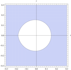
Figure 1: The constraint $|Kk^{2}/(s^{\mu}(1-\omega s^{-\rho})^{\gamma})|<1$ (blue region, with $x=\Re(s)$, $y=\Im(s)$) for $(K,k,\mu,\omega,\rho,\gamma)=(1,1,0.5,-1,0.25,1)$.

The abscissa $c$ clearly depends on $k$ which varies in $\mathbb{R}$ (notice however that $c$ does not depend on $n$). The inversion term by term of the Laplace transform is then permitted by Theorem 30.1 of Doetsch [8] and the series of the inverse transforms converges absolutely in $t\geq 0$ irrespective of the value of $c$ chosen (provided it is sufficently large).

In Fig. 2 it is possible to actually see the region of validity of the constraint $|\lambda(1-v)/(s^{\mu}(1+\phi s^{-\rho})^{\gamma})|<1$ for a specific choice of the parameters. As before, the application of the inverse Laplace transform term by term is ensured by Theorem 30.1 of Doetsch [8].

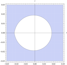
Figure 2: The constraint $|\lambda(1-v)/(s^{\mu}(1+\phi s^{-\rho})^{\gamma})|<1$ (blue region, with $x=\Re(s)$, $y=\Im(s)$) for $(\lambda,v,\mu,\phi,\rho,\gamma)=(1,0.5,0.5,1,0.25,1)$.

Acknowledgements

Živorad Tomovski has been supported by the Berlin Einstein Foundation through a Research Fellowship during his visit to the Weierstrass Institute for Applied Analysis and Stochastics in Berlin for three months during 2013.

Federico Polito has been supported by project AMALFI (Università di Torino/Compagnia di San Paolo).

References

- Al-Homidan et al. [2013] S. Al-Homidan, R. A. Ghanam and N. Tatar. On a generalized diffusion equation arising in petroleum engineering, Advances in Difference Equations, 349 (14 pages), 2013.
- Balakrishnan [1985] V. Balakrishnan, Anomalous diffusion in one dimension, Physica A, 132:569–580, 1985.
- Beghin and Macci [2012] L. Beghin and C. Macci. Large deviations for fractional Poisson processes, Statistics and Probability Letters, 83(4):1193–1202, 2012.
- Beghin and Orsingher [2009] L. Beghin and E. Orsingher. Fractional Poisson processes and related planar random motions, Electronic Journal of Probability, 14:1790–1826, 2009.
- Cahoy and Polito [2013] D.O. Cahoy and F. Polito. Renewal processes based on generalized Mittag–Leffler waiting times, Communications in Nonlinear Science and Numerical Simulation, 18(3):639–650, 2013.
- Dattoli et al. [1991] G. Dattoli, L. Gianessi, L. Mezi, D. Tocci and R. Colai. FEL time-evolution operator, Nucl. Instr. Methods A, 304:541–544, 1991.
- Diethelm [2010] K. Diethelm. The Analysis of Fractional Differential Equations, Springer, New York, 2010.
- Doetsch [1974] G. Doetsch. Introduction to the Theory and Application of the Laplace Transformation, Springer, New York, 1974.
- D’Ovidio and Polito [2013] M. D’Ovidio and F. Polito, Fractional Diffusion-Telegraph Equations and their Associated Stochastic Solutions, arXiv:1307.1696, 2013.
- Gnedenko and Kovalenko [1968] B.V. Gnedenko and I.N. Kovalenko: Introduction to Queueing Theory, Israel Program for Scientific Translations, Jerusalem 1968.
- Gorenflo and Mainardi [1997] R. Gorenflo and F. Mainardi. Fractional calculus: integral and differential equations of fractional order. In: A. Carpinteri and F. Mainardi Fractals and Fractional Calculus in Continuum Mechanics, 223–276, Springer-Verlag, Wien, 1997.
- Gorenflo and Mainardi [2013] R. Gorenflo and F. Mainardi. On the fractional Poisson process and the discretized stable subordinator, arXiv:1305.3074, 2013.
- Gorenflo and Mainardi [2012] R. Gorenflo and F. Mainardi. Laplace-Laplace analysis of the fractional Poisson process. In: S. Rogosin, AMADE. Papers and memoirs to the memory of Prof. Anatoly Kilbas, 43–58, Publishing House of BSU, Minsk, 2012.
- Gradshteyn and Ryzhik [2007] I.S. Gradshteyn and I.M. Ryzhik, Table of Integrals, Series, and Products, Seventh Edition, Elsevier Academic Press, (2007)
- Hilfer and Anton [1995] R. Hilfer and L. Anton, Fractional master equation and fractal time random walks. Physical Review E, 51:R848–R851, 1995.
- Hilfer [2000] R. Hilfer. Fractional calculus and regular variation in thermodynamics. In R. Hilfer, editor, Applications of Fractional Calculus in Physics, 429, Singapore, 2000. World Scientific.
- Hilfer [2008] R. Hilfer. Threefold introduction to fractional derivatives, Anomalous transport: Foundations and applications, 17–73, 2008.
- Kilbas et al. [2004] A.A. Kilbas, M. Saigo and R.K. Saxena. Generalized Mittag–Leffler function and generalized fractional calculus operators, Integral transform and special functions, 15(1):31–49, 2004.
- Kilbas et al. [2002] A.A. Kilbas, M. Saigo and R.K. Saxena. Solution of Volterra integro-differential equations with generalized Mittag–Leffler function in the kernels, Journal of integral equations and applications, 14(4):377–396, 2002.
- Kilbas et al. [2005] A.A. Kilbas, H.M. Srivastava and J.J. Trujillo. Theory and Applications of the Fractional Differential Equations, North-Holland Mathematics Studies, 204, 2006.
- Laskin [2003] N. Laskin. Fractional Poisson process, Communications in Nonlinear Science and Numerical Simulation, 8:201–213, 2003.
- Laskin [2009] N. Laskin. Some applications of the fractional Poisson probability distribution, Journal of Mathematical Physics, 50:113513, 2009.
- Luchko [2010] Y. Luchko. Some uniqueness and existence results for the initial-boundary-value problems for the generalized time-fractional diffusion equation, Computers & Mathematics with Applications, 59(5):1766–1772, 2010.
- Luchko [2011] Y. Luchko. Initial-boundary-value problems for the generalized multi-term time-fractional diffusion equation. Journal of Mathematical Analysis and Applications, 374(2):538–548, 2011.
- Mainardi [1997] F. Mainardi: Fractional Calculus. Some basic problems in continuum and statistical mechanics. In: A. Carpinteri and F. Mainardi (editors): Fractals and Fractional Calculus in Continuum Mechanics, 291–348. Springer Verlag, Wien, 1997
- Mainardi et al. [2000] F. Mainardi, M. Raberto, R. Gorenflo and E. Scalas: Fractional calculus and continuous time finance II: the waiting time distribution, Physica A, 287:468–481, 2000
- Mainardi et al. [2004a] F. Mainardi, R. Gorenflo and E. Scalas. A renewal process of Mittag–Leffler type. In: M. Novak, Thinking in Patterns: Fractals and Related Phenomena in Nature. World Scientific, Singapore 2004, 35–46, Vancouver, 2004.
- Mainardi et al. [2004b] F. Mainardi, R. Gorenflo, E. Scalas. A fractional generalization of the Poisson process, Vietnam Journal of Mathematics, 32:53–64, 2004.
- Mainardi et al. [2007] F. Mainardi, Y. Luchko, G. Pagnini. The fundamental solution of the space-time fractional diffusion equation, Fractional Calculus and Applied Analysis, 4(2):153–192, 2001.
- Meerschaert et al. [2011] M.M. Meerschaert, E. Nane and P. Vellaisamy. The Fractional Poisson Process and the Inverse Stable Subordinator, Electronic Journal of Probability 16(59):1600–1620, 2011.
- Orsingher and Polito [2012] E. Orsingher and F. Polito. The space-fractional Poisson process, Statistics and Probability Letters, 82(4):852–858, 2012.
- Orsingher and Polito [2013] E. Orsingher and F. Polito. On the integral of fractional Poisson processes, Statistics and Probability letters, 83:1006–1017, 2013.
- Podlubny [1999] I. Podlubny. Fractional Differential Equations, Academic Press, New York, 1999.
- Politi et al. [2011] M. Politi, T. Kaizoji and E. Scalas. Full characterization of the fractional Poisson process, EPL, 96:20004 (6 pages), 2011.
- Povstenko [2010] Y.Z. Povstenko. Evolution of the initial box-signal for time-fractional diffusion-wave equation in a case of different spatial dimensions. Physica A: Statistical Mechanics and its Applications, 389(21):4696–4707, 2010.
- Prabhakar [1971] T.R. Prabhakar. A singular integral equation with a generalized Mittag–Leffler function in the kernel, Yokohama Mathematical Journal, 19:7–15, 1971.
- Repin and Saichev [2000] O.N. Repin, A.I. Saichev. Fractional Poisson law, Radiophysics and Quantum Electronics, 43(9):738–741, 2000.
- Samko et al. [1993] S.G. Samko, A.A. Kilbas and O.I. Marichev. Fractional integrals and derivatives, Gordon and Breach Science, Yverdon, 1993.
- Sandev et al. [2011] T. Sandev, R. Metzler, and Ž. Tomovski. Fractional diffusion equation with a generalized Riemann–Liouville time fractional derivative, Journal of Physics A: Mathematical and Theoretical, 44(25):255203, 2011.
- Sandev et al. [2011] T. Sandev, Ž. Tomovski and J.L. Dubbeldam. Generalized Langevin equation with a three parameter Mittag–Leffler noise, Physica A: Statistical Mechanics and its Applications, 390(21):3627–3636, 2011.
- Schilling et al. [2012] R.L. Schilling, R. Song and Z. Vondracek. Bernstein functions: theory and applications, Walter de Gruyter, 2012.
- Sebastian and Gorenflo [2013] N. Sebastian and R. Gorenflo. A fractional generalization of the Poisson processes and some of its properties, arXiv:1307.8271, 2013.
- Srivastava and Tomovski [2009] H.M. Srivastava and Ž. Tomovski. Fractional calculus with an integral operator containing a generalized Mittag–Leffler function in the kernel, Applied Mathematics and Computation, 211(1):198–210, 2009.
- Tamarkin [1930] J.D. Tamarkin. On integrable solutions of Abel’s integral equations, Annals of Mathematics, 31:219–229, 1930.
- Tomovski et al. [2010] Ž. Tomovski, R. Hilfer and H.M. Srivastava. Fractional and operational calculus with generalized fractional derivative operators and Mittag–Leffler type functions, Integral Transforms and Special Functions, 21(11):797–814, 2010.
- Zhou and Jiao [2010] Y. Zhou and F. Jiao. Nonlocal Cauchy problem for fractional evolution equations, Nonlinear Analysis: Real World Applications, 11(5):4465–4475, 2010.