Safe Sample Screening for
Support Vector Machines

Abstract

Sparse classifiers such as the support vector machines (SVM) are efficient in test-phases because the classifier is characterized only by a subset of the samples called support vectors (SVs), and the rest of the samples (non SVs) have no influence on the classification result. However, the advantage of the sparsity has not been fully exploited in training phases because it is generally difficult to know which sample turns out to be SV beforehand. In this paper, we introduce a new approach called safe sample screening that enables us to identify a subset of the non-SVs and screen them out prior to the training phase. Our approach is different from existing heuristic approaches in the sense that the screened samples are guaranteed to be non-SVs at the optimal solution. We investigate the advantage of the safe sample screening approach through intensive numerical experiments, and demonstrate that it can substantially decrease the computational cost of the state-of-the-art SVM solvers such as LIBSVM. In the current big data era, we believe that safe sample screening would be of great practical importance since the data size can be reduced without sacrificing the optimality of the final solution.

I Introduction

The support vector machines (SVM) [1, 2, 3] has been successfully applied to large-scale classification problems [4, 5, 6]. A trained SVM classifier is sparse in the sense that the decision function is characterized only by a subset of the samples known as support vectors (SVs). One of the computational advantages of such a sparse classifier is its efficiency in the test phase, where the classifier can be evaluated for a new test input with the cost proportional only to the number of the SVs. The rest of the samples (non-SVs) can be discarded after training phases because they have no influence on the classification results.

However, the advantage of the sparsity has not been fully exploited in the training phase because it is generally difficult to know which sample turns out to be SV beforehand. Many existing SVM solvers spend most of their time for identifying the SVs [7, 8, 9, 10, 11]. For example, well-known LIBSVM [11] first predicts which sample would be SV (prediction step), and then solves a smaller optimization problem defined only with the subset of the samples predicted as SVs (optimization step). These two steps must be repeated until the true SVs are identified because some of the samples might be mistakenly predicted as non-SVs in the prediction step.

In this paper, we introduce a new approach that can identify a subset of the non-SVs and screen them out before actually solving the training optimization problem. Our approach is different from the prediction step in the above LIBSVM or other similar heuristic approaches in the sense that the screened samples are guaranteed to be non-SVs at the optimal solution. It means that the original optimal solution can be obtained by solving the smaller problem defined only with the remaining set of the non-screened samples. We call our approach as safe sample screening because it never identifies a true SV as non-SV. Figure1 illustrates our approach on a toy data set (see §V-A for details).

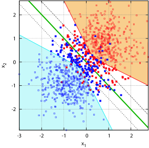
Figure 1: An example of our safe sample screening method on a binary classification problem with a two-dimensional toy data set. For each of the red and blue classes, 500 samples are drawn. Our safe sample screening method found that all the samples in the shaded regions are guaranteed to be non-SVs. In this example, more than 80% of the samples ($\square$ and $\square$) are identified as non-SVs and they can be discarded prior to the training phase. It means that the optimal classifier (the green line) can be obtained by solving a much smaller optimization problem defined only with the remaining 20% of the samples ($\blacksquare$ and $\blacksquare$). See §V-A for details.

Safe sample screening can be used together with any SVM solvers such as LIBSVM as a preprocessing step for reducing the training set size. In our experience, it is often possible to screen out nearly 90% of the samples as non-SVs. In such cases, the total computational cost of SVM training can be substantially reduced because only the remaining 10% of the samples are fed into an SVM solver (see §V). Furthermore, we show that safe sample screening is especially useful for model selection, where a sequence of SVM classifiers with different regularization parameters are trained. In the current big data era, we believe that safe sample screening would be of great practical importance because it enables us to reduce the data size without sacrificing the optimality.

The basic idea behind safe sample screening is inspired by a resent study by El Ghaoui et al. [12]. In the context of $L_{1}$ regularized sparse linear models, they introduced an approach that can safely identify a subset of the non-active features whose coefficients turn out to be zero at the optimal solution. This approach has been called safe feature screening, and various extensions have been reported [13, 14, 15, 16, 17, 18, 19, 20, 21] (see §IV-F for details). Our contribution is to extend the idea of [12] for safely screening out non-SVs. This extension is non-trivial because the feature sparseness in a linear model stems from the $L_{1}$ penalty, while the sample sparseness in an SVM is originated from the large-margin principle.

This paper is an extended version of our preliminary conference paper [22], where we proposed a safe sample screening method that can be used in somewhat more restricted situation than we consider here (see Appendix B for details). In this paper, we extend our previous method in order to overcome the limitation and to improve the screening performance. As the best of our knowledge, our approach in [22] is the first safe sample screening method. After our conference paper was published, Wang et al. [23] recently proposed a new method and demonstrated that it performed better than our previous method in [22]. In this paper, we further go beyond the Wang et al.’s method, and show that our new method has better screening performance from both theoretical and empirical viewpoints (see §IV-F for details).

The rest of the paper is organized as follows. In §II, we formulate the SVM and summarize the optimality conditions. Our main contribution is presented in §III where we propose three safe sample screening methods for SVMs. In §IV, we describe how to use the proposed safe sample screening methods in practice. Intensive experiments are conducted in §V, where we investigate how much the computational cost of the state-of-the-art SVM solvers can be reduced by using safe sample screening. We summarize our contribution and future works in §VI. Appendix contains the proofs of all the theorems and the lemmas, a brief description of (and comparison with) our previous method in our preliminary conference paper [22], the relationship between our methods and the method in [23], and some deitaled experimental protocols. The C++ and Matlab codes are available at http://www-als.ics.nitech.ac.jp/code/index.php?safe-sample-screening.

Notation: We let $\mathbb{R}$, $\mathbb{R}_{+}$ and $\mathbb{R}_{++}$ be the set of real, nonnegative and positive numbers, respectively. We define $\mathbb{N}_{n}\triangleq\{1,\ldots,n\}$ for any natural number $n$. Vectors and matrices are represented by bold face lower and upper case characters such as $\bm{v}\in\mathbb{R}^{n}$ and $\bm{M}\in\mathbb{R}^{m\times n}$, respectively. An element of a vector $\bm{v}$ is written as $v_{i}$ or $(\bm{v})_{i}$. Similarly, an element of a matrix $\bm{M}$ is written as $M_{ij}$ or $(\bm{M})_{ij}$. Inequalities between two vectors such as $\bm{v}\leq\bm{w}$ indicate component-wise inequalities: $v_{i}\leq w_{i}~{}\forall i\in\mathbb{N}_{n}$. Unless otherwise stated, we use $\|\cdot\|$ as a Euclidean norm. A vector of all 0 and 1 are denoted as $\mathbf{0}$ and $\mathbf{1}$, respectively.

II Support vector machine

In this section we formulate the support vector machine (SVM). Let us consider a binary classification problem with $n$ samples and $d$ features. We denote the training set as $\{(\bm{x}_{i},y_{i})\}_{i\in\mathbb{N}_{n}}$ where $\bm{x}_{i}\in{\cal X}\subseteq\mathbb{R}^{d}$ and $y_{i}\in\{-1,+1\}$. We consider a linear model in a feature space ${\cal F}$ in the following form:

$$f(\bm{x})=\bm{w}^{\top}\Phi(\bm{x}_{i}),$$

where $\Phi:{\cal X}\rightarrow{\cal F}$ is a map from the input space ${\cal X}$ to the feature space ${\cal F}$, and $\bm{w}\in{\cal F}$ is a vector of the coefficients. We sometimes write $f(\bm{x})$ as $f(\bm{x};\bm{w})$ for explicitly specifying the associated parameter $\bm{w}$. The optimal parameter $\bm{w}^{*}$ is obtained by solving

$$\bm{w}^{*}\triangleq\arg\min_{\bm{w}\in{\cal F}}~{}\frac{1}{2}\|\bm{w}\|^{2}+C\sum_{i\in\mathbb{N}_{n}}\max\{0,1-y_{i}f(\bm{x}_{i})\},$$ (1)

where $C\in\mathbb{R}_{++}$ is the regularization parameter. The loss function $\max\{0,1-y_{i}f(\bm{x}_{i})\}$ is known as hinge-loss. We use a notation such as $\bm{w}_{[C]}^{*}$ when we emphasize that it is the optimal solution of the problem (1) associated with the regularization parameter $C$.

The dual problem of (1) is formulated with the Lagrange multipliers $\bm{\alpha}\in\mathbb{R}_{+}^{n}$ as

$$\bm{\alpha}_{[C]}^{*}\triangleq\arg\max_{\bm{\alpha}}~{}\bigl{(}{\cal D}(\bm{\alpha})\triangleq-\frac{1}{2}\sum_{i,j\in\mathbb{N}_{n}}\alpha_{i}\alpha_{j}Q_{ij}+\sum_{i\in\mathbb{N}_{n}}\alpha_{i}\bigr{)}~{}~{}~{}\text{s.t.}~{}0\leq\alpha_{i}\leq C,i\in\mathbb{N}_{n},$$ (2)

where $\bm{Q}\in\mathbb{R}^{n\times n}$ is an $n\times n$ matrix defined as $Q_{ij}\triangleq y_{i}y_{j}K(\bm{x}_{i},\bm{x}_{j})$ and $K(\bm{x}_{i},\bm{x}_{j})\triangleq\Phi(\bm{x}_{i})^{\top}\Phi(\bm{x}_{j})$ is the Mercer kernel function defined by the feature map $\Phi$.

Using the dual variables, the model $f$ is written as

$$f(\bm{x})=\sum_{i\in\mathbb{N}_{n}}\alpha_{i}y_{i}K(\bm{x}_{i},\bm{x}).$$ (3)

Denoting the optimal dual variables as $\{\alpha^{*}_{[C]i}\}_{i\in\mathbb{N}_{n}}$, the optimality conditions of the SVM are summarized as

$$i\in{\cal R}\Rightarrow\alpha_{[C]i}^{*}=0,~{}~{}~{}i\in{\cal E}\Rightarrow\alpha_{[C]i}^{*}\in[0,C],~{}~{}~{}i\in{\cal L}\Rightarrow\alpha_{[C]i}^{*}=C,$$ (4)

where we define the three index sets:

$${\cal R}\triangleq\{i\in\mathbb{N}_{n}~{}|~{}y_{i}f(\bm{x}_{i})>1\},~{}~{}~{}{\cal E}\triangleq\{i\in\mathbb{N}_{n}~{}|~{}y_{i}f(\bm{x}_{i})=1\},~{}~{}~{}{\cal L}\triangleq\{i\in\mathbb{N}_{n}~{}|~{}y_{i}f(\bm{x}_{i})<1\}.$$

The optimality conditions (4) suggest that, if it is known a priori which samples turn out to be the members of ${\cal R}$ at the optimal solution, those samples can be discarded before actually solving the training optimization problem because the corresponding $\alpha^{*}_{[C]i}=0$ indicates that they have no influence on the solution. Similarly, if some of the samples are known a priori to be the members of ${\cal L}$ at the optimal solution, the corresponding variable can be fixed as $\alpha^{*}_{[C]i}=C$. If we let ${\cal R}^{\prime}$ and ${\cal L}^{\prime}$ be the subset of the samples known as the members of ${\cal R}$ and ${\cal L}$, respectively, one could first compute $d_{i}\triangleq C\sum_{j\in{\cal L}^{\prime}}y_{j}K(\bm{x}_{i},\bm{x}_{j})$ for all $i\in\mathbb{N}_{n}\setminus({\cal R}^{\prime}\cup{\cal L}^{\prime})$, and put them in a cache. Then, it is suffice to solve the following smaller optimization problem defined only with the remaining subset of the samples and the cached variables:

$$\max_{\bm{\alpha}}\sum_{i,j\in\mathbb{N}_{n}\setminus({\cal R}^{\prime}\cup{\cal L}^{\prime})}\!\!\!\!\!\alpha_{i}\alpha_{j}Q_{ij}-\sum_{i\in\mathbb{N}_{n}\setminus({\cal R}^{\prime}\cup{\cal L}^{\prime})}\!\!\!\!\!\alpha_{i}(1-d_{i})~{}~{}~{}{\rm s.t.}~{}0\leq\alpha_{i}\leq C,~{}i\in\mathbb{N}_{n}\setminus({\cal R}^{\prime}\cup{\cal L}^{\prime}).$$

Hereafter, the training samples in ${\cal E}$ are called support vectors (SVs), while those in ${\cal R}$ and ${\cal L}$ are called non-support vectors (non-SVs). Note that support vectors usually indicate the samples both in ${\cal E}$ and ${\cal L}$ in the machine learning literature (we also use the term SVs in this sense in the previous section). We adopt the above uncommon terminology because the samples in ${\cal R}$ and ${\cal L}$ can be treated almost in an equal manner in the rest of this paper. In the next section, we develop three types of testing procedures for screening out a subset of the non-SVs. Each of these tests are conducted by evaluating a simple rule for each sample. We call these testing procedures as safe sample screening tests and the associated rules as safe sample screening rules.

III Safe Sample Screening for SVMs

In this section, we present our safe sample screening approach for SVMs.

III-A Basic idea

Let us consider a situation that we have a region $\Theta_{[C]}\subset{\cal F}$ in the solution space, where we only know that the optimal solution $\bm{w}^{*}_{[C]}$ is somewhere in this region $\Theta_{[C]}$, but $\bm{w}^{*}_{[C]}$ itself is unknown. In this case, the optimality conditions (4) indicate that

$$\bm{w}^{*}_{[C]}\in\Theta_{[C]}~{}\wedge~{}\min_{\bm{w}\in\Theta_{[C]}}y_{i}f(\bm{x}_{i};\bm{w})>1~{}\Rightarrow~{}y_{i}f(\bm{x}_{i};\bm{w}^{*}_{[C]})>1~{}\Rightarrow~{}\alpha_{[C]i}^{*}=0.$$ (5)

$$\bm{w}^{*}_{[C]}\in\Theta_{[C]}~{}\wedge~{}\max_{\bm{w}\in\Theta_{[C]}}y_{i}f(\bm{x}_{i};\bm{w})<1~{}\Rightarrow~{}y_{i}f(\bm{x}_{i};\bm{w}^{*}_{[C]})<1~{}\Rightarrow~{}\alpha_{[C]i}^{*}=C.$$ (6)

These facts imply that, even if the optimal $\bm{w}^{*}_{[C]}$ itself is unknown, we might have a chance to screen out a subset of the samples in ${\cal R}$ or ${\cal L}$.

Based on the above idea, we construct safe sample screening rules in the following way:

(Step 1)

we construct a region $\Theta_{[C]}$ such that

$$\bm{w}^{*}_{[C]}\in\Theta_{[C]}\subset{\cal F}.$$ (7)

(Step 2)

we compute the lower and the upper bounds:

$$\ell_{[C]i}\triangleq\min_{\bm{w}\in\Theta_{[C]}}y_{i}f(\bm{x}_{i};\bm{w}),~{}~{}~{}u_{[C]i}\triangleq\max_{\bm{w}\in\Theta_{[C]}}y_{i}f(\bm{x}_{i};\bm{w})~{}~{}~{}\forall i\in\mathbb{N}_{n}.$$ (8)

Then, the safe sample screening rules are written as

$$\ell_{[C]i}>1~{}\Rightarrow~{}i\in{\cal R}~{}\Rightarrow~{}\alpha^{*}_{[C]i}=0,~{}~{}~{}u_{[C]i}<1~{}\Rightarrow~{}i\in{\cal L}~{}\Rightarrow~{}\alpha^{*}_{[C]i}=C.$$ (9)

In section III-B, we first study so-called Ball Test where the region $\Theta_{[C]}$ is a closed ball in the solution space. In this case, the lower and the upper bounds can be obtained in closed forms. In section III-C, we describe how to construct such a ball $\Theta_{[C]}$ for SVMs, and introduce two types of balls $\Theta_{[C]}^{\rm(BT1)}$ and $\Theta_{[C]}^{\rm(BT2)}$. We call the corresponding tests as Ball Test 1 (BT1) and Ball Test 2 (BT2), respectively. In section III-D, we combine these two balls and develop so-called Intersection Test (IT), which is shown to be more powerful (more samples can be screened out) than BT1 and BT2.

III-B Ball Test

When $\Theta_{[C]}$ is a closed ball, the lower or the upper bounds of $y_{i}f(\bm{x}_{i})$ can be obtained by minimizing a linear objective subject to a single quadratic constraint. We can easily show that the solution of this class of optimization problems is given in a closed form [24].

Lemma 1 (Ball Test)

Let $\Theta_{[C]}\subset{\cal F}$ be a ball with the center $\bm{m}\in{\cal F}$ and the radius $r\in\mathbb{R}_{+}$, i.e., $\Theta_{[C]}\triangleq\{\bm{w}\in{\cal F}~{}|~{}\|\bm{w}-\bm{m}\|\leq r\}$. Then, the lower and the upper bounds in (8) are written as

$$\ell_{[C]i}\equiv\min_{\bm{w}\in\Theta_{[C]}}y_{i}f(\bm{x}_{i};\bm{w})=\bm{z}_{i}^{\top}\bm{m}-r\|\bm{z}_{i}\|,~{}~{}~{}u_{[C]i}\equiv\max_{\bm{w}\in\Theta_{[C]}}y_{i}f(\bm{x}_{i};\bm{w})=\bm{z}_{i}^{\top}\bm{m}+r\|\bm{z}_{i}\|,$$ (10)

where we define $\bm{z}_{i}\triangleq y_{i}\Phi(\bm{x}_{i})$, $i\in\mathbb{N}_{n}$, for notational simplicity.

The proof is presented in Appendix A. The geometric interpretation of Lemma 1 is shown in Figure2.

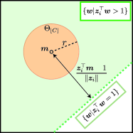
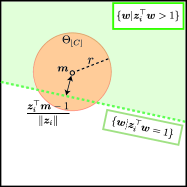
(a) Success	(b) Fail

Figure 2: A geometric interpretation of ball tests. Two panels illustrate the solution space when the $i^{\rm th}$ sample (a) can be screened out, and (b) cannot be screened out, respectively. In both panels, the dotted green line indicates the hyperplane $y_{i}f(\bm{x}_{i};\bm{w})\equiv\bm{z}_{i}^{\top}\bm{w}=1$, and the green region represents $\{\bm{w}|\bm{z}_{i}^{\top}\bm{w}>1\}$. The orange circle with the center $\bm{m}$ and the radius $r$ is the ball region $\Theta_{[C]}$ in which the optimal solution $\bm{w}^{*}_{[C]}$ exists. In (a), the fact that the hyperplane $\bm{z}_{i}^{\top}\bm{w}=1$ does not intersect with $\Theta_{[C]}$, i.e., the distance $(\bm{z}_{i}^{\top}\bm{m}-1)/||\bm{z}_{i}||$ is larger than the radius $r$, implies that $y_{i}f(\bm{x}_{i};\bm{w}^{*}_{[C]})>1$ wherever the optimal solution $\bm{w}^{*}_{[C]}$ locates within the region $\Theta_{[C]}$, and the $i^{\rm th}$ sample can be screened out as a member of ${\cal R}$. On the other hand, in (b), the hyperplane $\bm{z}_{i}^{\top}\bm{w}=1$ intersects with $\Theta_{[C]}$, meaning that we do not know whether $y_{i}f(\bm{x}_{i};\bm{w}^{*}_{[C]})>1$ or not until we actually solve the optimization problem and obtain the optimal solution $\bm{w}^{*}_{[C]}$.

III-C Ball Tests for SVMs

The following problem is shown to be equivalent to (1) in the sense that $\bm{w}^{*}_{[C]}$ is the optimal solution of the original SVM problem (1):

$$(\bm{w}^{*}_{[C]},\xi^{*}_{[C]})\triangleq\arg\!\!\!\!\!\min_{\bm{w}\in{\cal F},\xi\in\mathbb{R}}\!\!\!{\cal P}_{[C]}(\bm{w},\xi)\triangleq\frac{1}{2}\|\bm{w}\|^{2}+C\xi~{}{\rm s.t.}~{}\xi\geq\sum_{i\in\mathbb{N}_{n}}s_{i}(1-y_{i}f(\bm{x}_{i}))~{}\forall\bm{s}\in\{0,1\}^{n}.~{}$$ (11)

We call the solution space of (11) as expanded solution space. In the expanded solution space, a quadratic function is minimized over a polyhedron composed of $2^{n}$ closed half spaces.

In the following lemma, we consider a specific type of regions in the expanded solution space. By projecting the region onto the original solution space, we have a ball region in the form of Lemma 1.

Lemma 2

Consider a region in the following form:

$$\Theta^{\prime}_{[C]}\triangleq\Big{\{}(\bm{w},\xi)\in{\cal F}\times\mathbb{R}~{}\Big{|}~{}a_{1}\|\bm{w}\|^{2}+\bm{b}_{1}^{\top}\bm{w}+c_{1}+\xi\leq 0,~{}\bm{b}_{2}^{\top}\bm{w}+c_{2}\leq\xi\Big{\}},$$ (12)

where $a_{1}\in\mathbb{R}_{++}$, $\bm{b}_{1},\bm{b}_{2}\in{\cal F}$, $c_{1},c_{2}\in\mathbb{R}$. If $\Theta^{\prime}_{[C]}$ is non-empty and $(\bm{w},\xi)\in\Theta^{\prime}_{[C]}$, $\bm{w}$ is in a ball $\Theta_{[C]}$ with the center $\bm{m}\in{\cal F}$ and the radius $r\in{\cal R}_{+}$ defined as

$$\bm{m}\triangleq-\frac{1}{2a_{1}}(\bm{b}_{1}+\bm{b}_{2}),~{}r\triangleq\sqrt{\|\bm{m}\|^{2}-\frac{1}{a_{1}}(c_{1}+c_{2}).}$$

The proof is presented in Appendix A. The lemma suggests that a Ball Test can be constructed by introducing two types of necessary conditions in the form of quadratic and linear constraints in (12). In the following three lemmas, we introduce three types of necessary conditions for the optimal solution $(\bm{w}^{*}_{[C]},\xi^{*}_{[C]})$ of the problem (11).

Lemma 3 (Necessary Condition 1 (NC1))

Let $(\tilde{\bm{w}},\tilde{\xi})$ be a feasible solution of (11). Then,

$$\frac{1}{C}\|\bm{w}^{*}_{[C]}\|^{2}-\frac{1}{C}\tilde{\bm{w}}^{\top}\bm{w}^{*}_{[C]}-\tilde{\xi}+\xi^{*}_{[C]}\leq 0.$$ (13)

Lemma 4 (Necessary Condition 2 (NC2))

Let $(\bm{w}^{*}_{[\check{C}]},\xi^{*}_{[\check{C}]})$ be the optimal solution for any other regularization parameter $\check{C}\in\mathbb{R}_{++}$. Then,

$$-\frac{1}{\check{C}}\bm{w}_{[\check{C}]}^{*\top}\bm{w}^{*}_{[C]}+\frac{1}{\check{C}}\|\bm{w}^{*}_{[\check{C}]}\|^{2}+\xi^{*}_{[\check{C}]}\leq\xi^{*}_{[C]}.$$ (14)

Lemma 5 (Necessary Condition 3 (NC3))

Let $\hat{\bm{s}}\in\{0,1\}^{n}$ be an $n$-dimensional binary vector. Then,

$$-\bm{z}_{\hat{\bm{s}}}^{\top}\bm{w}^{*}_{[C]}+\hat{\bm{s}}^{\top}\mathbf{1}\leq\xi^{*}_{[C]},\text{ where }\bm{z}_{\hat{\bm{s}}}\triangleq\sum_{i\in\mathbb{N}_{n}}\hat{s}_{i}\bm{z}_{i}.$$ (15)

The proofs of these three lemmas are presented in Appendix A. Note that NC1 is quadratic, while NC2 and NC3 are linear constraints in the form of (12). As described in the following theorems, Ball Test 1 (BT1) is constructed by using NC1 and NC2, while Ball Test 2 (BT2) is constructed by using NC1 and NC3.

Theorem 6 (Ball Test 1 (BT1))

Let $(\tilde{\bm{w}},\tilde{\xi})$ be any feasible solution and $(\bm{w}^{*}_{[\check{C}]},\xi^{*}_{[\check{C}]})$ be the optimal solution of (11) for any other regularization parameter $\check{C}$. Then, the optimal SVM solution $\bm{w}^{*}_{[C]}$ is included in the ball $\Theta^{\rm(BT1)}_{[C]}\triangleq\{\bm{w}~{}\big{|}~{}\|\bm{w}-\bm{m}_{1}\|\leq r_{1}\}$, where

$$\bm{m}_{1}\triangleq\frac{1}{2}(\tilde{\bm{w}}+\frac{C}{\check{C}}\bm{w}^{*}_{[\check{C}]}),~{}r_{1}\triangleq\sqrt{\|\bm{m}_{1}\|^{2}-\frac{C}{\check{C}}\|\bm{w}^{*}_{[\check{C}]}\|^{2}+C(\tilde{\xi}-\xi^{*}_{[\check{C}]})}.$$ (16)

By applying the ball $\Theta^{\rm(BT1)}_{[C]}$ to Lemma 1, we can compute the lower bound $\ell^{\rm(BT1)}_{[C]}$ and the upper bound $u^{\rm(BT1)}_{[C]}$.

Theorem 7 (Ball Test 2 (BT2))

Let $(\tilde{\bm{w}},\tilde{\xi})$ be any feasible solution of (11) and $\hat{\bm{s}}$ be any $n$-dimensional binary vector in $\{0,1\}^{n}$. Then, the optimal SVM solution $\bm{w}^{*}_{[C]}$ is included in the ball $\Theta^{\rm(BT2)}_{[C]}\triangleq\{\bm{w}~{}\big{|}~{}\|\bm{w}-\bm{m}_{2}\|\leq r_{2}\}$, where

$$\bm{m}_{2}\triangleq\frac{1}{2}(\tilde{\bm{w}}+C\bm{z}_{\hat{\bm{s}}}),~{}r_{2}\triangleq\sqrt{\|\bm{m}_{2}\|^{2}+C(\tilde{\xi}-\hat{\bm{s}}^{\top}\mathbf{1})}.$$

By applying the ball $\Theta^{\rm(BT2)}_{[C]}$ to Lemma 1, we can compute the lower bound $\ell^{\rm(BT2)}_{[C]}$ and the upper bound $u^{\rm(BT2)}_{[C]}$.

III-D Intersection Test

We introduce a more powerful screening test called Intersection Test (IT) based on

$$\Theta_{[C]}^{\rm(IT)}\triangleq\Theta_{[C]}^{\rm(BT1)}\cap\Theta_{[C]}^{\rm(BT2)}.$$

Theorem 8 (Intersection Test)

The lower and the upper bounds of $y_{i}f(\bm{x}_{i};\bm{w})$ in $\Theta_{[C]}^{\rm(IT)}$ are

$$\ell^{\rm(IT)}_{[C]i}\triangleq\min_{\bm{w}\in\Theta_{[C]}^{\rm(IT)}}y_{i}f(\bm{x}_{i};\bm{w})=\left\{\begin{array}[]{ll}\ell^{\rm(BT1)}_{[C]i}&\text{ if }\frac{-\bm{z}_{i}^{\top}\bm{\phi}}{\|\bm{z}_{i}\|~{}\|\bm{\phi}\|}<\frac{\zeta-\|\bm{\phi}\|}{r_{1}},\\ \ell^{\rm(BT2)}_{[C]i}&\text{ if }\frac{\zeta}{r_{2}}<\frac{-\bm{z}_{i}^{\top}\bm{\phi}}{\|\bm{z}_{i}\|~{}\|\bm{\phi}\|},\\ \bm{z}_{i}^{\top}\bm{\psi}-\kappa\sqrt{\|\bm{z}_{i}\|^{2}-\frac{(\bm{z}_{i}^{\top}\bm{\phi})^{2}}{\|\bm{\phi}\|^{2}}}&\text{ if }\frac{\zeta-\|\bm{\phi}\|}{r_{1}}\leq\frac{-\bm{z}_{i}^{\top}\bm{\phi}}{\|\bm{z}_{i}\|~{}\|\bm{\phi}\|}\leq\frac{\zeta}{r_{2}}\end{array}\right.$$ (20)

and

$$u^{\rm(IT)}_{[C]i}\triangleq\max_{\bm{w}\in\Theta_{[C]}^{\rm(IT)}}y_{i}f(\bm{x}_{i};\bm{w})=\left\{\begin{array}[]{ll}u^{\rm(BT1)}_{[C]i}&\text{ if }\frac{\bm{z}_{i}^{\top}\bm{\phi}}{\|\bm{z}_{i}\|~{}\|\bm{\phi}\|}<\frac{\zeta-\|\bm{\phi}\|}{r_{1}},\\ u^{\rm(BT2)}_{[C]i}&\text{ if }\frac{\zeta}{r_{2}}<\frac{\bm{z}_{i}^{\top}\bm{\phi}}{\|\bm{z}_{i}\|~{}\|\bm{\phi}\|},\\ \bm{z}_{i}^{\top}\bm{\psi}+\kappa\sqrt{\|\bm{z}_{i}\|^{2}-\frac{(\bm{z}_{i}^{\top}\bm{\phi})^{2}}{\|\bm{\phi}\|^{2}}}&\text{ if }\frac{\zeta-\|\bm{\phi}\|}{r_{1}}\leq\frac{\bm{z}_{i}^{\top}\bm{\phi}}{\|\bm{z}_{i}\|~{}\|\bm{\phi}\|}\leq\frac{\zeta}{r_{2}},\end{array}\right.$$ (24)

where

$$\bm{\phi}\triangleq\bm{m}_{1}-\bm{m}_{2},~{}\zeta\triangleq\frac{1}{2\|\bm{\phi}\|}(\|\bm{\phi}\|^{2}+r_{2}^{2}-r_{1}^{2}),~{}\bm{\psi}\triangleq\bm{m}_{2}+\zeta\bm{\phi}/\|\bm{\phi}\|,~{}\kappa\triangleq\sqrt{r_{2}^{2}-\zeta^{2}}.$$

The proof is presented in Appendix A. Note that IT is guaranteed to be more powerful than BT1 and BT2 because $\Theta^{\rm(IT)}_{[C]}$ is the intersection of $\Theta^{\rm(BT1)}_{[C]}$ and $\Theta^{\rm(BT2)}_{[C]}$.

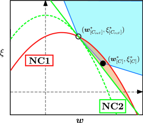
Figure 3: A schematic illustration of the two necessary conditions NC1 and NC2 in the expanded solution space when we use the reference solution $(\bm{w}^{*}_{[C_{\rm ref}]},\xi^{*}_{[C_{\rm ref}]})$. The blue polytope in the upper-right corner indicates the feasible region of (11). The open circle $\circ$ and the filled circle $\bullet$ indicate the optimal solutions $(\bm{w}^{*}_{[C_{\rm ref}]},\xi^{*}_{[C_{\rm ref}]})$ and $(\bm{w}^{*}_{[C]},\xi^{*}_{[C]})$, respectively. The red quadratic curve and green line indicate the boundaries of NC1 and NC2, respectively. Note that the green line is the tangent at the point $(\bm{w}^{*}_{[C_{\rm ref}]},\xi^{*}_{[C_{\rm ref}]})$ of the objective function ${\cal P}_{[C_{\rm ref}]}(\bm{w},\xi)$ which is shown by green dotted quadratic curve. The area surrounded by the red quadratic curve and the green line is the region $\Theta^{\prime}_{C}$ in which the optimal solution $(\bm{w}^{*}_{[C]},\xi^{*}_{[C]})$, exists.

IV Safe Sample Screening in Practice

In order to use the safe sample screening methods in practice, we need two additional side information: a feasible solution $(\tilde{\bm{w}},\tilde{\xi})$ and the optimal solution $(\bm{w}^{*}_{[\check{C}]},\xi^{*}_{[\check{C}]})$ for a different regularization parameter $\check{C}$. Hereafter, we focus on a particular situation that the optimal solution $\bm{w}^{*}_{[C_{\rm ref}]}$ for a smaller $C_{\rm ref}<C$ is available, and call such a solution as a reference solution. We later see that such a reference solution can be easily available in practical model building process. Let $\xi^{*}_{[C_{\rm ref}]}\triangleq\sum_{i\in\mathbb{N}_{n}}\max\{0,1-y_{i}f(\bm{x}_{i};\bm{w}^{*}_{[C_{\rm ref}]})\}$. By replacing both of $(\tilde{\bm{w}},\tilde{\xi})$ and $(\bm{w}^{*}_{[\check{C}]},\xi^{*}_{[\check{C}]})$ with $(\bm{w}^{*}_{[C_{\rm ref}]},\xi^{*}_{[C_{\rm ref}]})$, the centers and the radiuses of $\Theta^{\rm(BT1)}_{[C]}$ and $\Theta^{\rm(BT1)}_{[C]}$ are rewritten as

$$\bm{m}_{1}=\frac{C+C_{\rm ref}}{2C_{\rm ref}}\bm{w}^{*}_{[C_{\rm ref}]},r_{1}=\frac{C-C_{\rm ref}}{2C_{\rm ref}}\|\bm{w}^{*}_{[C_{\rm ref}]}\|,$$

$$\bm{m}_{2}=\frac{1}{2}(\bm{w}^{*}_{[C_{\rm ref}]}+C\bm{z}_{\hat{\bm{s}}}),r_{2}=\sqrt{\|\bm{m}_{2}\|^{2}+C(\xi^{*}_{[C_{\rm ref}]}-\hat{\bm{s}}^{\top}\bm{1})}.$$

A geometric interpretation of the two necessary conditions NC1 and NC2 in this special case is illustrated in Figure3. In the rest of this section, we discuss how to obtain reference solutions and other practical issues.

IV-A How to obtain a reference solution

The following lemma implies that, for a sufficiently small regularization parameter $C$, we can make use of a trivially obtainable reference solution.

Lemma 9

Let $C_{\rm min}\triangleq 1/\max_{i\in\mathbb{N}_{n}}(\bm{Q}\mathbf{1})_{i}$. Then, for $C\in(0,C_{\rm min}]$, the optimal solution of the dual SVM formulation (2) is written as $\bm{\alpha}^{*}_{[C]}=C\mathbf{1}$.

The proof is presented in Appendix A. Without loss of generality, we only consider the case with $C>C_{\rm min}$, where we can use the solution $\bm{w}^{*}_{[C_{\rm min}]}$ as the reference solution.

IV-B Regularization path computation

In model selection process, a sequence of SVM classifiers with various different regularization parameters $C$ are trained. Such a sequence of the solutions is sometimes referred to as regularization path [9, 27]. Let us write the sequence as $C_{1}<\ldots<C_{T}$. We note that SVM is easier to train (the convergence tends to be faster) for smaller regularization parameter $C$. Therefore, it is reasonable to compute the regularization path from smaller $C$ to larger $C$ with the help of warm-start approach [28], where the previous optimal solution at $C_{t-1}$ is used as the initial starting point of the next optimization problem for $C_{t}$. In such a situation, we can make use of the previous solution at $C_{t-1}$ as the reference solution. Note that this is more advantageous than using $C_{\rm min}$ as the reference solution because the rules can be more powerful when the reference solution is closer to $\bm{w}^{*}_{[C]}$. Moreover, the rule evaluation cost can be reduced in regularization path computation scenario (see IV-E).

IV-C How to select $\hat{\bm{s}}$ for the necessary condition 3

We discuss how to select $\hat{\bm{s}}\in\{0,1\}^{n}$ for NC3. Since a smaller region leads to a more powerful rule, it is reasonable to select $\hat{\bm{s}}\in\{0,1\}^{n}$ so that the volume of the intersection region $\Theta_{[C]}^{\rm(IT)}\equiv\Theta_{[C]}^{\rm(BT1)}\cup\Theta_{[C]}^{\rm(BT2)}$ is as small as possible. We select $\hat{\bm{s}}$ such that the distance between the two balls $\Theta^{\rm(BT1)}_{[C]}$ and $\Theta^{\rm(BT2)}_{[C]}$ is maximized, while the radius of $\Theta^{\rm(BT2)}_{[C]}$ is minimized, i.e.,

$$\hat{\bm{s}}=\arg\max_{\bm{s}\in\{0,1\}^{n}}\left(\|\bm{m}_{1}-\bm{m}_{2}\|^{2}-r_{2}^{2}\right)=\arg\max_{\bm{s}\in\{0,1\}^{n}}\sum_{i\in\mathbb{N}_{n}}s_{i}(1-\frac{C+C_{\rm ref}}{2C_{\rm ref}}y_{i}f(\bm{x}_{i};\bm{w}_{[C_{\rm ref}]}^{*})).$$ (25)

Note that the solution of (25) can be straightforwardly obtained as

$$\hat{s}_{i}=I\{1-\frac{C+C_{\rm ref}}{2C_{\rm ref}}y_{i}f(\bm{x}_{i};\bm{w}_{[C_{\rm ref}]}^{*})>0\},~{}i\in\mathbb{N}_{n},$$

where $I(\cdot)$ is the indicator function.

IV-D Kernelization

The proposed safe sample screening rules can be kernelized, i.e., all the computations can be carried out without explicitly working on the high-dimensional feature space ${\cal F}$. Remembering that $Q_{ij}=\bm{z}_{i}^{\top}\bm{z}_{j}\equiv y_{i}\Phi(\bm{x}_{i})^{\top}\Phi(\bm{x}_{j})y_{j}$, we can rewrite the rules by using the following relations:

$$\|\bm{z}_{i}\|=\sqrt{Q_{ii}},~{}\|\bm{w}_{[C_{\rm ref}]}^{*}\|=\sqrt{\bm{\alpha}_{[C_{\rm ref}]}^{*\top}\bm{Q}\bm{\alpha}_{[C_{\rm ref}]}^{*}},~{}\bm{z}_{i}^{\top}\bm{m}_{1}=\frac{C+C_{\rm ref}}{2C_{\rm ref}}(\bm{Q}\bm{\alpha}^{*}_{[C_{\rm ref}]})_{i},$$

$$\bm{z}_{i}^{\top}\bm{m}_{2}=\frac{1}{2}(\bm{Q}\bm{\alpha}^{*}_{[C_{\rm ref}]})_{i}+\frac{C}{2}(\bm{Q}\hat{\bm{s}})_{i},~{}\|\bm{m}_{1}\|=\frac{C+C_{\rm ref}}{2C_{\rm ref}}\sqrt{\bm{\alpha}^{*\top}_{[C_{\rm ref}]}\bm{Q}\bm{\alpha}^{*}_{[C_{\rm ref}]}},$$

$$\|\bm{m}_{2}\|=\frac{1}{2}\sqrt{(\bm{\alpha}^{*}_{[C_{\rm ref}]}+C\hat{\bm{s}})^{\top}\bm{Q}(\bm{\alpha}^{*}_{[C_{\rm ref}]}+C\hat{\bm{s}})},~{}\bm{m}_{1}^{\top}\bm{m}_{2}=\frac{C+C_{\rm ref}}{4C_{\rm ref}}(\bm{\alpha}^{*\top}_{[C_{\rm ref}]}\bm{Q}\bm{\alpha}^{*}_{[C_{\rm ref}]}+C\bm{\alpha}^{*\top}_{[C_{\rm ref}]}\bm{Q}\hat{\bm{s}}).$$

Exploiting the sparsities of $\bm{\alpha}_{[C_{\rm ref}]}^{*}$ and $\hat{\bm{s}}$, some parts of the rule evaluations can be done efficiently (see §IV-E for details).

IV-E Computational Complexity

The computational complexities for evaluating the safe sample screening rules are summarized in Table I. Note that the rule evaluation cost can be reduced in regularization path computation scenario. The bottleneck of the rule evaluation is in the computation of $\bm{\alpha}_{[C_{\rm ref}]}^{*\top}\bm{Q}\bm{\alpha}_{[C_{\rm ref}]}^{*}$. Since many SVM solvers (including LIBLINEAR and LIBSVM) use the value $\bm{Q}\bm{\alpha}$ in their internal computation and store it in a cache, we can make use of the cache value for circumventing the bottleneck. Furthermore, BT2 (and henceforth IT) can be efficiently computed in regularization path computation scenario by caching $\bm{Q}\hat{\bm{s}}$.

TABLE I: The computational complexities of the rule evaluations

	linear	kernel	kernel (cache)
BT1	$\mathcal{O}(nd_{s})$	$\mathcal{O}(n^{2})$	$\mathcal{O}(n)$
BT2	$\mathcal{O}(nd_{s})$	$\mathcal{O}(n^{2})$	$\mathcal{O}(n\|\Delta\hat{\bm{s}}\|_{0})$
IT	$\mathcal{O}(nd_{s})$	$\mathcal{O}(n^{2})$	$\mathcal{O}(n\|\Delta\hat{\bm{s}}\|_{0})$

For each of Ball Test 1 (BT1), Ball Test 2 (BT2), and Intersection Test (IT), the complexities for evaluating the safe sample screening rules for all $i\in\mathbb{N}_{n}$ of linear SVM and nonlinear kernel SVM (with and without using the cache values as discussed in §IV-B) are shown. Here, $d_{s}$ indicates the average number of non-zero features for each sample and $\|\Delta\hat{\bm{s}}\|_{0}$ indicates the number of different elements in $\hat{\bm{s}}$ between two consecutive $C_{t-1}$ and $C_{t}$ in regularization path computation scenario.

IV-F Relation with existing approaches

This work is highly inspired by the safe feature screening introduced by El Ghaoui et al. [12]. After the seminal work by El Ghaoui et al. [12], many efforts have been devoted for improving screening performances [13, 14, 15, 16, 17, 18, 19, 20, 21]. All the above listed studies are designed for screening the features in $L_{1}$ penalized linear model .

As the best of our knowledge, the approach presented in our conference paper [22] is the first safe sample screening method that can safely eliminate a subset of the samples before actually solving the training optimization problem. Note that this extension is non-trivial because the feature sparseness in a linear model stems from the $L_{1}$ penalty, while the sample sparseness in an SVM is originated from the large-margin principle.

After our conference paper [22] was published, Wang et al. [23] recently proposed a method called DVI test, and showed that it is more powerful than our previous method in [22]. In this paper, we further go beyond the DVI test. We can show that DVI test is equivalent to Ball Test 1 (BT1) in a special case (the equivalence is shown in Appendix C). Since the region $\Theta^{\rm(IT)}_{[C]}$ is included in the region $\Theta^{\rm(BT1)}_{[C]}$, Intersection Test (IT) is theoretically guaranteed to be more powerful than DVI test. We will also empirically demonstrate that IT consistently outperforms DVI test in terms of screening performances in §V.

One of our non-trivial contributions is in §III-C, where a ball-form region is constructed by first considering a region in the expanded solution space and then projecting it onto the original solution space. The idea of merging two balls for constructing the intersection region in §III-D is also our original contribution. We conjecture that the basic idea of Intersection Test can be also useful for safe feature screening.

V Experiments

We demonstrate the advantage of the proposed safe sample screening methods through numerical experiments. We first describe the problem setup of Figure1 in §V-A. In §V-B, we report the screening rates, i.e., how many percent of the non-SVs can be screened out by safe sample screening. In §V-C, we show that the computational cost of the state-of-the-art SVM solvers (LIBSVM [11] and LIBLINEAR [30] ) can be substantially reduced with the use of safe sample screening. Note that DVI test proposed in [23] is identical with BT1 in all the experimental setups considered here (see Appendix C). Table II summarizes the benchmark data sets used in our experiments.

TABLE II: Benchmark data sets used in the experiments

Data Set	#samples ($n$)	#features ($d$)
D01: B.C.D	569	30
D02: dna	2,000	180
D03: DIGIT1	1,500	241
D04: satimage	4,435	36
D05: gisette	6,000	5,000
D06: mushrooms	8,124	112
D07: news20	19,996	1,355,191
D08: shuttle	43,500	9
D09: acoustic	78,832	50
D10: url	2,396,130	3,231,961
D11: kdd-a	8,407,752	20,216,830
D12: kdd-b	19,264,097	29,890,095

We refer D01 $\sim$ D04 as small, D05 and D08 as medium, and D09 $\sim$ D12 as large data sets. We only used linear kernel for large data sets because the kernel matrix computation for $n>50,000$ is computationally prohibitive.

V-A Artificial toy example in Figure1

The data set $\{(\bm{x}_{i},y_{i})\}_{i\in\mathbb{N}_{1000}}$ in Figure1 was generated as

$$\bm{x}_{i}\sim N([-0.5,-0.5]^{\top},1.5^{2}\bm{I})\text{ and }y_{i}=-1~{}\text{for odd}~{}i,$$

$$\bm{x}_{i}\sim N([+0.5,+0.5]^{\top},1.5^{2}\bm{I})\text{ and }y_{i}=+1~{}\text{for even}~{}i,$$

where $\bm{I}$ is the identity matrix. We considered the problem of learning a linear classifier at $C=10$. Intersection Test was conducted by using the reference solution at $C_{\rm ref}=5$. For the purpose of illustration, Figure1 only highlights the area in which the samples are screened out as the members of ${\cal R}$ (red and blue shaded regions).

V-B Screening rate

We report the screening rates of BT1, BT2 and IT. The screening rate is defined as the number of the screened samples over the total number of the non-SVs (both in ${\cal R}$ and ${\cal L}$). The rules were constructed by using the optimal solution at $C_{\rm ref}(<C)$ as the reference solution. We used linear kernel and RBF kernel $K(\bm{x},\bm{x}^{\prime})=\exp(-\gamma\|\bm{x}-\bm{x}^{\prime}\|^{2})$ where $\gamma\in\{0.1/d,1/d,10/d\}$ is a kernel parameter and $d$ is the input dimension.

Due to the space limitation, we only show the results on four small data sets with $C=10$ in Figure4. In each plot, the horizontal axis denotes $C_{\rm ref}/C\in(0,1]$. In most cases, the screening rates increased as $C_{\rm ref}/C$ increases from 0 to 1, i.e., the rules are more powerful when the reference solution $\bm{w}^{*}_{[C_{\rm ref}]}$ is closer to $\bm{w}^{*}_{[C]}$. The screening rates of IT were always higher than those of BT1 and BT2 because $\Theta^{\rm(IT)}_{[C]}$ is shown to be smaller than $\Theta^{\rm(BT1)}_{[C]}$ and $\Theta^{\rm(BT2)}_{[C]}$ by construction. The three tests behaved similarly in other problem setups.

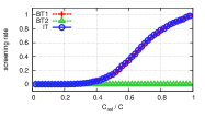
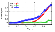
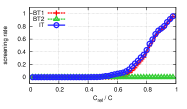
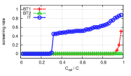
D01, Linear	D01, RBF ($\gamma=0.1/d$)	D01, RBF ($\gamma=1/d$)	D01, RBF ($\gamma=10/d$)
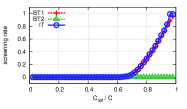
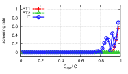
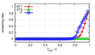
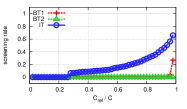
D02, Linear	D02, RBF ($\gamma=0.1/d$)	D02, RBF ($\gamma=1/d$)	D02, RBF ($\gamma=10/d$)
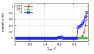
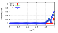
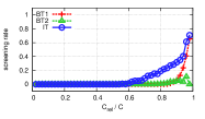
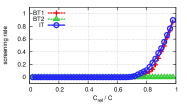
D03, Linear	D03, RBF ($\gamma=0.1/d$)	D03, RBF ($\gamma=1/d$)	D03, RBF ($\gamma=10/d$)
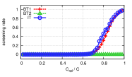
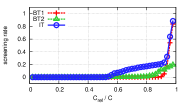
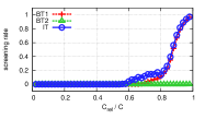
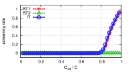
D04, Linear	D04, RBF ($\gamma=0.1/d$)	D04, RBF ($\gamma=1/d$)	D04, RBF ($\gamma=10/d$)

Figure 4: The screening rates of the three proposed safe screening tests BT1 (red), BT2 (green) and IT (blue).

V-C Computation time

We investigate how much the computational cost of the entire SVM training process can be reduced by safe sample screening. As the state-of-the-art SVM solvers, we used LIBSVM [11] and LIBLINEAR [30] for nonlinear and linear kernel cases, respectively. Many SVM solvers use non-safe sample screening heuristics in their inner loops. The common basic idea in these heuristic approaches is to predict which sample turns out to be SV or non-SV (prediction step), and to solve a smaller optimization problem defined only with the subset of the samples predicted as SVs (optimization step). These two steps must be repeated until all the optimality conditions in (4) are satisfied because the prediction step in these heuristic approaches is not safe. In LIBSVM and LIBLINEAR, such a heuristic is called shrinking.

We compared the total computational costs of the following six approaches:

• Full-sample training (Full),

• Shrinking (Shrink),

• Ball Test 1 (BT1),

• Shrinking + Ball Test 1 (Shrink+BT1).

• Intersection Test (IT),

• Shrinking + Intersection Test (Shrink+IT).

In Full and Shrink, we used LIBSVM or LIBLINEAR with and without shrinking option, respectively. In BT1 and Shrink+BT1, we first screened out a subset of the samples by Ball Test 1, and the rest of the samples were fed into LIBSVM or LIBLINEAR to solve the smaller optimization problem with and without shrinking option, respectively. In IT and Shrink+IT, we used Intersection Test for safe sample screening.

V-C1 Single SVM training

First, we compared the computational costs of training a single linear SVM for the large data sets ($n>50,000$). Here, our task was to find the optimal solution at the regularization parameter $C=C_{\rm ref}/0.9$ using the reference solution at $C_{\rm ref}=500C_{\rm min}$.

Table III shows the average computational costs of 5 runs. The best performance was obtained in all the setups when both shrinking and IT screening are simultaneously used (Shrink+IT). Shrink+BT1 also performed well, but it was consistently outperformed by Shrink+IT.

TABLE III: The computation time [sec] for training a single SVM.

	LIBLINEAR		Safe Sample Screening
Data set	Full	Shrink	BT1	Shrink+BT1	Rule	Rate	IT	Shrink+IT	Rule	Rate
D09	98.2	2.57	95.1	2.21	0.0022	0.178	47.3	1.21	0.0214	0.51
D10	1881	327	1690	247	0.0514	0.108	1575	228	2.24	0.125
D11	2801	115	2699	97.2	0.203	0.136	2757	88.1	2.78	0.136
D12	16875	4558	7170	4028	0.432	0.138	12002	3293	5.39	0.139

The computation time of the best approach in each setup is written in boldface. Rule and Rate indicate the computation time and the screening rate of the each rules, respectively.

V-C2 Regularization path

As described in §IV-B, safe sample screening is especially useful in regularization path computation scenario. When we compute an SVM regularization path for an increasing sequence of the regularization parameters $C_{1}<\ldots<C_{T}$, the previous optimal solution can be used as the reference solution. We used a recently proposed $\varepsilon$-approximation path ($\varepsilon$-path) algorithm [34, 27] for setting a practically meaningful sequence of regularization parameters. The detail $\varepsilon$-approximation path procedure is described in Appendix D.

TABLE IV: The computation time [sec] for computing regularization path.

		LIBSVM or LIBLINEAR		Safe Sample Screening
Data set	Kernel	Full	Shrink	BT1	Shrink+BT1	IT	Shrink+IT
	Linear	389	35.2	174	34.8	177	34.8
D01	RBF($0.1/d$)	43.8	4.51	9.08	2.8	8.48	2.87
	RBF($1/d$)	2.73	0.68	0.435	0.295	0.464	0.294
	RBF($10/d$)	0.73	0.4	0.312	0.221	0.266	0.213
	Linear	67	9.09	13.6	8.05	13.4	8.14
D02	RBF($0.1/d$)	298	106	253	87.7	242	80.7
	RBF($1/d$)	13.9	5.27	7.14	2.5	7.03	2.62
	RBF($10/d$)	4.98	2.68	3.18	1.96	2.71	1.82
	Linear	369	59.3	221	56.7	167	56.9
D03	RBF($0.1/d$)	938	261	928	262	741	203
	RBF($1/d$)	94.3	27.3	70.9	19.4	60.7	16.8
	RBF($10/d$)	6.93	2.71	2.92	0.77	2.45	0.794
	Linear	3435	33.7	3256	33.2	3248	33.2
D04	RBF($0.1/d$)	1365	565	1325	547	1178	488
	RBF($1/d$)	635	218	392	129	277	88.7
	RBF($10/d$)	31	20.4	3.89	1.5	3.87	1.68
	Linear	1532	350	894	318	899	329
D05	RBF($0.1/d$)	375	143	365	132	296	103
	RBF($1/d$)	63.9	30.1	33.4	13.5	25.4	10.2
	RBF($10/d$)	34.3	20.7	27.8	16.8	24.9	15.9
	Linear	19.8	2.64	8.12	2.08	8.57	2.03
D06	RBF($0.1/d$)	1938	618	1838	572	1395	423
	RBF($1/d$)	239	103	164	62.3	134	50.6
	RBF($10/d$)	94.3	56.3	70.5	44.2	66.2	40.9
	Linear	2619	1665	2495	1697	2427	1769
D07	RBF($0.1/d$)	10358	5565	10239	5493	10245	5770
	RBF($1/d$)	33960	12797	34019	12918	30373	10152
	RBF($10/d$)	270984	67348	270313	67062	264433	56427
	Linear	37135	67	35945	63.6	36386	67.8
D08	RBF($0.1/d$)	278232	63192	275688	63608	253219	51932
	RBF($1/d$)	214165	60608	203155	56161	180839	48867
	RBF($10/d$)	167690	54364	129490	45644	125675	44463

The computation time of the best approach in each setup is written in boldface.

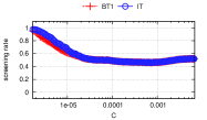
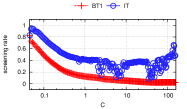
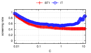
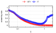
D05, Linear	D05, RBF ($\gamma=0.1/d$)	D05, RBF ($\gamma=1/d$)	D05, RBF ($\gamma=10/d$)
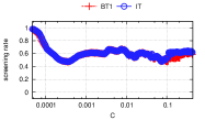
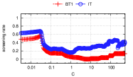
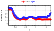
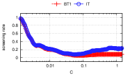
D06, Linear	D06, RBF ($\gamma=0.1/d$)	D06, RBF ($\gamma=1/d$)	D06, RBF ($\gamma=10/d$)
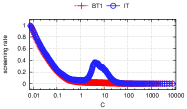
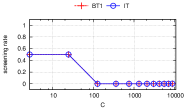
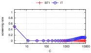
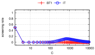
D07, Linear	D07, RBF ($\gamma=0.1/d$)	D07, RBF ($\gamma=1/d$)	D07, RBF ($\gamma=10/d$)
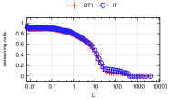
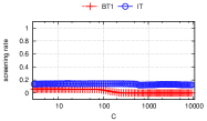
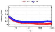
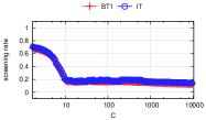
D08, Linear	D08, RBF ($\gamma=0.1/d$)	D08, RBF ($\gamma=1/d$)	D08, RBF ($\gamma=10/d$)

Figure 5: The screening rate in regularization path computation scenario for BT1 (red) and IT (blue).

In this scenario, we used the small and the medium data sets ($n\leq 50,000$). The largest regularization parameter was set as $C_{T}=10^{4}$. We used linear kernel and RBF kernel $K(\bm{x},\bm{x}^{\prime})=\exp(-\gamma\|\bm{x}-\bm{x}^{\prime}\|^{2})$ with $\gamma\in\{0.1/d,1/d,10/d\}$. In all the six approaches, we used the cache value and warm-start approach as described in §IV-B. Table IV summarizes the total computation time of the six approaches, and Figure5 shows how screening rates change with $C$ in each data set (due to the space limitation, we only show the results on four medium data sets in Figure5).

Note first that shrinking heuristic was very helpful, and safe sample screening alone (BT1 and IT) was not as effective as shrinking. However, except one setup (D07, Linear), simultaneously using shrinking and safe sample screening worked better than using shrinking alone. As we discuss in §IV-E, the rule evaluation cost of BT1 is cheaper than that of IT. Therefore, if the screening rates of these two tests are same, the former is slightly faster than the latter. In Table IV, we see that Shrink+BT1 was a little faster than Shrink+IT in several setups. We conjecture that those small differences are due to the differences in the rule evaluation costs. In the remaining setups, Shrink+IT was faster than Shrink+BT1. The differences tend to be small in the cases of linear kernel and RBF kernel with relatively small $\gamma$. On the other hand, significant improvements were sometimes observed especially when RBF kernels with relatively large $\gamma$ is used. In Figure 5, we confirmed that the screening rates of IT was never worse than BT1.

In summary, the experimental results indicate that safe sample screening is often helpful for reducing the computational cost of the state-of-the-art SVM solvers. Furthermore, Intersection Test seems to be the best safe sample screening method among those we considered here.

VI Conclusion

In this paper, we introduced safe sample screening approach that can safely identify and screen out a subset of the non-SVs prior to the training phase. We believe that our contribution would be of great practical importance in the current big data era because it enables us to reduce the data size without sacrificing the optimality. Our approach is quite general in the sense that it can be used together with any SVM solvers as a preprocessing step for reducing the data set size. The experimental results indicate that safe sample screening is not so harmful even when it cannot screen out any instances because the rule evaluation costs are much smaller than that of SVM solvers. Since the screening rates highly depend on the choice of the reference solution, an important future work is to find a better reference solution.

Appendix A Proofs

Proof:

The lower bound $\ell_{[C]i}$ is obtained as follows:

$$\min_{\bm{w}}~{}y_{i}f(\bm{x}_{i};\bm{w})~{}{\rm s.t.}~{}\|\bm{w}-\bm{m}\|^{2}\leq r^{2}=\min_{\bm{w}}\max_{\mu>0}~{}\bm{z}_{i}^{\top}\bm{w}+\mu(\|\bm{w}-\bm{m}\|^{2}-r^{2})$$

$$= \max_{\mu>0}~{}(-\mu r^{2})+\min_{\bm{w}}~{}(\mu\|\bm{w}-\bm{m}\|^{2}+\bm{z}_{i}^{\top}\bm{w})=\max_{\mu>0}~{}L(\mu)\triangleq-\mu r^{2}-\frac{\|\bm{z}_{i}\|^{2}}{4\mu}+\bm{z}_{i}^{\top}\bm{m},$$

where the Lagrange multiplier $\mu>0$ because the ball constraint is strictly active when the bound is attained. By solving $\partial L(\mu)/\partial\mu=0$, the optimal Lagrange multiplier is given as $\mu=\|\bm{z}_{i}\|/2r$. Substituting this into $L(\mu)$, we obtain

$$\max_{\mu\geq 0}L(\mu)=\bm{z}_{i}^{\top}\bm{m}-r\|\bm{z}_{i}\|.$$

The upper bound $u_{[C]i}$ is obtained similarly. ∎

Proof:

By substituting $\xi$ in the second inequality in (12) into the first inequality, we immediately have $\|\bm{w}-\bm{m}\|\leq r$. ∎

Proof:

From Proposition 2.1.2 in [35], the optimal solution $(\bm{w}^{*}_{[C]},\xi^{*}_{[C]})$ and a feasible solution $(\tilde{\bm{w}},\tilde{\xi})$ satisfy the following relationship:

$$\nabla{\cal P}_{[C]}(\bm{w}^{*}_{[C]},\xi^{*}_{[C]})^{\top}\left(\left[\begin{array}[]{c}\tilde{\bm{w}}\\ \tilde{\xi}\\ \end{array}\right]-\left[\begin{array}[]{c}\bm{w}_{[C]}^{*}\\ \xi_{[C]}^{*}\\ \end{array}\right]\right)=\left[\begin{array}[]{cc}\bm{w}_{[C]}^{*\top}&C\end{array}\right]\left(\left[\begin{array}[]{c}\tilde{\bm{w}}\\ \tilde{\xi}\\ \end{array}\right]-\left[\begin{array}[]{c}\bm{w}_{[C]}^{*}\\ \xi_{[C]}^{*}\\ \end{array}\right]\right)\geq 0.$$

∎

Proof:

From Proposition 2.1.2 in [35], the optimal solution $(\bm{w}^{*}_{[C_{\rm ref}]},\xi^{*}_{[C_{\rm ref}]})$ and a feasible solution $(\bm{w}^{*}_{[C]},\xi^{*}_{[C]})$ satisfy the following relationship:

$$\nabla{\cal P}_{[\check{C}]}(\bm{w}^{*}_{[\check{C}]},\xi^{*}_{[\check{C}]})^{\top}\left(\left[\begin{array}[]{c}\bm{w}_{[C]}^{*}\\ \xi_{[C]}^{*}\\ \end{array}\right]-\left[\begin{array}[]{c}\bm{w}_{[\check{C}]}^{*}\\ \xi_{[\check{C}]}^{*}\\ \end{array}\right]\right)=\left[\begin{array}[]{cc}\bm{w}_{[\check{C}]}^{*\top}&\check{C}\end{array}\right]\left(\left[\begin{array}[]{c}\bm{w}_{[C]}^{*}\\ \xi_{[C]}^{*}\\ \end{array}\right]-\left[\begin{array}[]{c}\bm{w}_{[\check{C}]}^{*}\\ \xi_{[\check{C}]}^{*}\\ \end{array}\right]\right)\geq 0.$$

∎

Proof:

(15) is necessary for the optimal solution just because it is one of the $2^{n}$ constraints in (11). ∎

Proof:

First, we prove the following lemma.

Lemma 10

Let $\overline{\bm{w}}\in{\cal F}$ be the optimal solution of

$$\min_{\bm{w}}~{}\bm{z}_{i}^{\top}\bm{w}~{}{\rm s.t.}~{}\|\bm{w}-\bm{m}_{1}\|^{2}\leq r_{1}^{2},~{}\|\bm{w}-\bm{m}_{2}\|^{2}\leq r_{2}^{2},$$ (28)

and $(\underline{\bm{w}},\underline{\xi})\in{\cal F}\times\mathbb{R}$ be the optimal solution of

$$\min_{\bm{w},\xi}~{}\bm{z}_{i}^{\top}\bm{w}~{}{\rm s.t.}~{}\|\bm{w}\|^{2}\leq\xi,~{}\xi\leq 2\bm{m}_{1}^{\top}\bm{w}+r_{1}^{2}-\|\bm{m}_{1}\|^{2},~{}\xi\leq 2\bm{m}_{2}^{\top}\bm{w}+r_{2}^{2}-\|\bm{m}_{2}\|^{2}.$$ (29)

Then, the two optimization problems (28) and (29) are equivalent in the sense that $\bm{z}_{i}^{\top}\overline{\bm{w}}=\bm{z}_{i}^{\top}\underline{\bm{w}}$.

Proof:

Let $\overline{\xi}\triangleq\|\overline{\bm{w}}\|^{2}$. Then, $(\overline{\bm{w}},\overline{\xi})$ is a feasible solution of (29) because

$$\|\overline{\bm{w}}-\bm{m}_{1}\|^{2}\leq r_{1}^{2}~{}\Rightarrow~{}2\bm{m}_{1}^{\top}\overline{\bm{w}}+r_{1}^{2}-\|\bm{m}_{1}\|^{2}\geq\|\overline{\bm{w}}\|^{2}=\overline{\xi},$$

$$\|\overline{\bm{w}}-\bm{m}_{2}\|^{2}\leq r_{2}^{2}~{}\Rightarrow~{}2\bm{m}_{2}^{\top}\overline{\bm{w}}+r_{2}^{2}-\|\bm{m}_{2}\|^{2}\geq\|\overline{\bm{w}}\|^{2}=\overline{\xi}.$$

On the other hand, $(\underline{\bm{w}},\underline{\xi})$ is a feasible solution of (28) because

$$\|\underline{\bm{w}}\|^{2}\leq\underline{\xi}\text{ and }\underline{\xi}\leq 2\bm{m}_{1}^{\top}\underline{\bm{w}}+r_{1}^{2}-\|\bm{m}_{1}\|^{2}~{}\Rightarrow~{}\|\underline{\bm{w}}-\bm{m}_{1}\|^{2}\leq r_{1}^{2},$$

$$\|\underline{\bm{w}}\|^{2}\leq\underline{\xi}\text{ and }\underline{\xi}\leq 2\bm{m}_{2}^{\top}\underline{\bm{w}}+r_{2}^{2}-\|\bm{m}_{2}\|^{2}~{}\Rightarrow~{}\|\underline{\bm{w}}-\bm{m}_{2}\|^{2}\leq r_{2}^{2}.$$

These facts indicate that $\bm{z}_{i}^{\top}\overline{\bm{w}}=\bm{z}_{i}^{\top}\underline{\bm{w}}$ for arbitrary $\bm{z}_{i}\in{\cal F}$. ∎

We first note that at least one of the two balls $\Theta^{\rm(BT1)}_{[C]i}$ and $\Theta^{\rm(BT2)}_{[C]i}$ are strictly active when the lower bound is attained. It means that we can only consider the following three cases:

• Case 1) $\Theta^{\rm(BT1)}_{[C]i}$ is active and $\Theta^{\rm(BT2)}_{[C]i}$ is inactive,

• Case 2) $\Theta^{\rm(BT2)}_{[C]i}$ is active and $\Theta^{\rm(BT1)}_{[C]i}$ is inactive, and

• Case 3) Both $\Theta^{\rm(BT1)}_{[C]i}$ and $\Theta^{\rm(BT2)}_{[C]i}$ are active.

From Lemma 10, the lower bound $\ell^{\rm(IT)}_{[C]i}$ is the solution of

$$\min_{\bm{w},\xi}~{}\bm{z}_{i}^{\top}\bm{w}~{}{\rm s.t.}~{}\|\bm{w}\|^{2}\leq\xi,~{}\xi\leq 2\bm{m}_{1}^{\top}\bm{w}+r_{1}^{2}-\|\bm{m}_{1}\|^{2},~{}\xi\leq 2\bm{m}_{2}^{\top}\bm{w}+r_{2}^{2}-\|\bm{m}_{2}\|^{2}.$$ (30)

Introducing the Lagrange multipliers $\mu,\nu_{1},\nu_{2}\in\mathbb{R}_{+}$ for the three constraints in (30), we write the Lagrangian of the problem (30) as $L(\bm{w},\xi,\mu,\nu_{1},\nu_{2})$. From the stationary conditions, we have

$${\frac{\partial L}{\partial\bm{w}}}=0~{}\Leftrightarrow~{}\bm{w}=\frac{1}{2\mu}(2\nu_{1}\bm{m}_{1}+2\nu_{2}\bm{m}_{2}-\bm{z}_{i}),~{}{\frac{\partial L}{\partial\xi}}=0~{}\Leftrightarrow~{}\mu-\nu_{1}-\nu_{2}=0.$$ (31)

where $\mu>0$ because at least one of the two balls $\Theta^{\rm(BT1)}_{[C]i}$ and $\Theta^{\rm(BT2)}_{[C]i}$ are strictly active.

Case 1) Let us first consider the case where $\Theta^{\rm(BT1)}_{[C]i}$ is active and $\Theta^{\rm(BT2)}_{[C]i}$ is inactive, i.e., $\|\bm{w}-\bm{m}_{1}\|^{2}=r_{1}^{2}$ and $\|\bm{w}-\bm{m}_{2}\|^{2}<r_{2}^{2}$. Noting that $\nu_{2}=0$, the latter can be rewritten as

$$\|\bm{w}-\bm{m}_{2}\|^{2}<r_{2}^{2}~{}\Leftrightarrow~{}\frac{-\bm{z}_{i}^{\top}\bm{\phi}}{\|\bm{z}_{i}\|\|\bm{\phi}\|}<\frac{\zeta-\|\bm{\phi}\|}{r_{1}},$$

where we have used the stationary condition in (31). In this case, it is clear that the lower bound is identical with that of BT1, i.e., $\ell^{\rm{(IT)}}_{[C]i}=\ell^{\rm{(BT1)}}_{[C]i}$.

Case 2) Next, let us consider the case where $\Theta^{\rm(BT2)}_{[C]i}$ is active and $\Theta^{\rm(BT1)}_{[C]i}$ is inactive, i.e., $\|\bm{w}-\bm{m}_{2}\|^{2}=r_{2}^{2}$ and $\|\bm{w}-\bm{m}_{1}\|^{2}<r_{1}^{2}$. In the same way as Case 1), the latter condition is rewritten as

$$\|\bm{w}-\bm{m}_{1}\|^{2}<r_{1}^{2}~{}\Leftrightarrow~{}\frac{\zeta}{r_{2}}<\frac{-\bm{z}_{i}^{\top}\bm{\phi}}{\|\bm{z}_{i}\|\|\bm{\phi}\|}.$$

In this case, the lower bound of IT is identical with that of BT2, i.e., $\ell^{\rm{(IT)}}_{[C]i}=\ell^{\rm{(BT2)}}_{[C]i}$.

Case 3) Finally, let us consider the remaining case where both of the two balls $\Theta^{\rm(BT1)}_{[C]i}$ and $\Theta^{\rm(BT2)}_{[C]i}$ are strictly active. From the conditions of Case 1) and Case 2), the condition of Case 3) is written as

$$\frac{\zeta-\|\bm{\phi}\|}{r_{1}}\leq\frac{-\bm{z}_{i}^{\top}\bm{\phi}}{\|\bm{z}_{i}\|\|\bm{\phi}\|}\leq\frac{\zeta}{r_{2}}.$$ (32)

After plugging the stationary conditions (31) into $L(\bm{w},\xi,\mu,\nu_{1},\nu_{2})$, the solution of the following linear system of equations

$${\frac{\partial L}{\partial\mu}}=0,~{}{\frac{\partial L}{\partial\nu_{1}}}=0,~{}{\frac{\partial L}{\partial\nu_{2}}}=0,$$

are given as

$$\mu=\frac{1}{2\kappa}\sqrt{\|\bm{z}_{i}\|^{2}-\frac{(\bm{z}_{i}^{\top}\bm{\phi})^{2}}{\|\bm{\phi}\|^{2}}},~{}\nu_{1}=\mu\frac{\zeta}{\|\bm{\phi}\|}+\frac{\bm{z}_{i}^{\top}\bm{\phi}}{2\|\bm{\phi}\|^{2}},~{}\nu_{2}=\mu-\nu_{1}.$$ (33)

From (32), $\mu,\nu_{1},\nu_{2}$ in (33) are shown to be non-negative, meaning that (33) are the optimal Lagrange multipliers. By plugging these $\mu,\nu_{1},\nu_{2}$ into $\bm{w}$ in (31), the lower bound is obtained as

$$\ell_{i}^{\rm(IT)}=\bm{z}_{i}^{\top}\bm{\psi}-\kappa\sqrt{\|\bm{z}_{i}\|^{2}-\frac{(\bm{z}_{i}^{\top}\bm{\phi})^{2}}{\|\bm{\phi}\|^{2}}}.$$

By combining all the three cases above, the lower bound (20) is asserted. The upper bound (24) can be similarly derived. ∎

Proof:

It is suffice to show that $\bm{\alpha}=C\mathbf{1}$ satisfies the optimality condition for any $C\in(0,C_{min}]$. Remembering that $f(\bm{x}_{i})=\sum_{j\in\mathbb{N}_{n}}\alpha_{j}y_{j}K(\bm{x}_{i},\bm{x}_{j})=C(\bm{Q}\mathbf{1})_{i}$, we have

$$\max_{i\in\mathbb{N}_{n}}y_{i}f(\bm{x}_{i})=\max_{i\in\mathbb{N}_{n}}C(\bm{Q}\mathbf{1})_{i}\leq C_{\rm min}\max_{i\in\mathbb{N}_{n}}(\bm{Q}\mathbf{1})_{i}=1.$$

Noting that positive semi-definiteness of the matrix $\bm{Q}$ indicates $\mathbf{1}^{\top}\bm{Q}\mathbf{1}\geq 0$, the above inequality holds because at least one component of $\bm{Q}\mathbf{1}$ must have nonnegative value. It implies that all the $n$ samples are in either ${\cal E}$ or ${\cal L}$, where $\alpha_{i}=C~{}\forall i\in\mathbb{N}_{n}$ clearly satisfies the optimality. ∎

Appendix B A comparison with the method in [22]

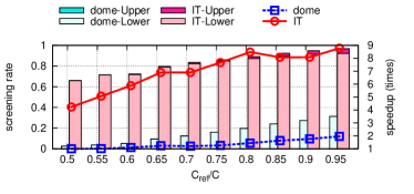
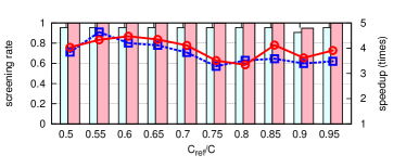
B.C.D. ($n=569,d=30$)	PCMAC ($n=1946,d=7511$)
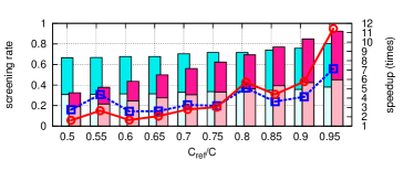
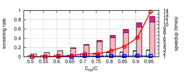
MAGIC. ($n=19020,d=10$)	IJCNN1 ($n=19990,d=22$)

Figure 6: The comparison between Intersection Test and Dome Test [22]. The red and blue bars (the left vertical axis) indicate the screening rates, i.e., the number of screened samples in ${\cal R}$ and ${\cal L}$ out of the total size $|{\cal R}|+|{\cal L}|$. The red and blue lines (the right vertical axis) show the speedup improvement, where the baseline is naive full-sample training without any screening.

We briefly describe the safe sample screening method proposed in our preliminary conference paper [22], which we call, Dome Test (DT). We discuss the difference among DT and IT, and compare their screening rates and computation times in simple numerical experiments. DT is summarized in the following theorem:

Theorem 11 (Dome Test)

Consider two positive scalars $C_{a}<C_{b}$. Then, for any $C\in[C_{a},C_{b}]$, the lower and the upper bounds of $y_{i}f(\bm{x}_{i};\bm{w}^{*}_{[C]})$ are given by

$$\ell_{[C]i}^{\rm(DT)}\triangleq\min_{\bm{w}\in\Theta}y_{i}f(\bm{x}_{i};\bm{w})=\left\{\begin{array}[]{ll}-\sqrt{2\gamma_{b}}\|\bm{z}_{i}\|&\text{if}~{}{\scriptstyle\frac{-\bm{z}_{i}^{\top}\bm{w}_{[C_{a}]}^{*}}{\|\bm{z}_{i}\|}}\geq{\scriptstyle\frac{\gamma_{a}\sqrt{2}}{\sqrt{\gamma_{b}}}}\\ \bm{z}_{i}^{\top}\bm{w}_{[C_{a}]}^{*}-\sqrt{{\scriptstyle\frac{\gamma_{b}-\gamma_{a}}{\gamma_{a}}}(\gamma_{a}\|\bm{z}_{i}\|^{2}-(\bm{z}_{i}^{\top}\bm{w}_{[C_{a}]}^{*})^{2}}&\text{otherwise}.\end{array}\right.$$

and

$$u_{[C]i}^{\rm(DT)}\triangleq\max_{\bm{w}\in\Theta}y_{i}f(\bm{x}_{i};\bm{w})=\left\{\begin{array}[]{ll}\sqrt{2\gamma_{b}}\|\bm{z}_{i}\|&\text{if}~{}{\scriptstyle\frac{\bm{z}_{i}^{\top}\bm{w}_{[C_{a}]}^{*}}{\|\bm{z}_{i}\|}}\geq{\scriptstyle\frac{\gamma_{a}\sqrt{2}}{\sqrt{\gamma_{b}}}}\\ \bm{z}_{i}^{\top}\bm{w}_{[C_{a}]}^{*}+\sqrt{{\scriptstyle\frac{\gamma_{b}-\gamma_{a}}{\gamma_{a}}}(\gamma_{a}\|\bm{z}_{i}\|^{2}-(\bm{z}_{i}^{\top}\bm{w}_{[C_{a}]}^{*})^{2}}&\text{otherwise},\end{array}\right.$$

where $\gamma_{a}\triangleq\|\bm{w}_{[C_{a}]}^{*}\|^{2}$ and $\gamma_{b}=\|\bm{w}_{[C_{b}]}^{*}\|^{2}$.

See [22] for the proof. A limitation of DT is that we need to know a feasible solution with a larger $C_{b}>C$ as well as the optimal solution with a smaller $C_{a}<C$ (remember that we only need the latter for BT1, BT2 and IT). As discussed in §IV-B, we usually train an SVM regularization path from smaller $C$ to larger $C$ by using warm-start approach. Therefore, it is sometimes computationally expensive to obtain a feasible solution with a larger $C_{b}>C$. In [22], we have used a bit tricky algorithm for obtaining such a feasible solution.

Figure6 shows the results of empirical comparison among DT and IT on the four data sets used in [22] with linear kernel (CVX [36] is used as the SVM solver in order to simply compare the effects of the screening performances). Here, we fixed $C_{\rm ref}=C_{a}=10^{4}C_{\rm min}$ and varied $C$ in the range of $[0.5C_{\rm ref},0.95C_{\rm ref}]$. For DT, we assumed that the optimal solution with $C_{b}=1.3C$ can be used as a feasible solution although it is a bit unfair setup for IT. We see that, IT is clearly better in B.C.D. and IJCNN1, comparable in PCMAC and slightly worse in MAGIC data sets albeit a bit unfair setup for IT. The reason why DT behaved poorly even when $C_{\rm ref}/C$ is close to 1 is that the lower and the upper bounds in DT depends on the value $(\gamma_{b}-\gamma_{a})/\gamma_{a}$, and does not depend on $C$ itself. It means that, when the range $[C_{a},C_{b}]$ is somewhat large, the performance of DT deteriorate.

Appendix C Equivalence between a special case of BT1 and the method in Wang et al. [23]

When we use the reference solution $\bm{w}^{*}_{[C_{\rm ref}]}$ as both of the feasible solution and the (different) optimal solution, the lower bound by BT1 is written as

$$\ell^{\rm(BT1)}_{[C]i}=\frac{C+C_{\rm ref}}{2C_{\rm ref}}\bm{z}_{i}^{\top}\bm{w}^{*}_{[C_{\rm ref}]}-\frac{C-C_{\rm ref}}{2C_{\rm ref}}\|\bm{w}^{*}_{[C_{\rm ref}]}\|\|\bm{z}_{i}\|$$

Using the relationships described in §IV-D, the dual form of the lower bound is written as

$$\ell^{\rm(BT1)}_{[C]i}=\frac{C+C_{\rm ref}}{2C_{\rm ref}}(\bm{Q}\bm{\alpha}^{*}_{[C_{\rm ref}]})_{i}-\frac{C-C_{\rm ref}}{2C_{\rm ref}}\sqrt{\bm{\alpha}^{*\top}_{[C_{\rm ref}]}\bm{Q}\bm{\alpha}^{*}_{[C_{\rm ref}]}Q_{ii}}.$$ (34)

After transforming some variables, (34) is easily shown to be equivalent to the first equation in Corollary 11 in [23]. Note that we derive BT1 in the primal solution space, while Wang et al. [23] derived the identical test in the dual space.

Appendix D $\varepsilon$-approximation Path Procedure

The $\varepsilon$-path algorithm enables us to compute an SVM regularization path such that the relative approximation error between two consecutive solutions are bounded by a small constant $\varepsilon$ (we set $\varepsilon=10^{-3}$). Precisely speaking, the sequence of the regularization parameters $\{C_{t}\}_{t\in\mathbb{N}_{T}}$ produced by the $\varepsilon$-path algorithm has a property that, for any $C_{t-1}$ and $C_{t}$, $t\in\{2,\ldots,T\}$, the former dual optimal solution $\bm{\alpha}^{*}_{C_{t-1}}$ satisfies

$$\frac{|{\cal D}(\bm{\alpha}_{[C]}^{*})-{\cal D}({\scriptstyle\frac{C}{C_{t-1}}}\bm{\alpha}_{[C_{t-1}]}^{*})|}{{\cal D}(\bm{\alpha}_{[C]}^{*})}\leq\varepsilon~{}\forall~{}C\in[C_{t-1},C_{t}],$$ (35)

where ${\cal D}$ is the dual objective function defined in (2). This property roughly implies that, the optimal solution $\bm{\alpha}^{*}_{[C_{t-1}]}$ is a reasonably good approximate solutions within the range of $C\in[C_{t-1},C_{t}]$.

Algorithm 1 describes the regularization path computation procedure with the safe sample screening and the $\varepsilon$-path algorithms. Given $\bm{w}^{*}_{[C_{t-1}]}$, the $\varepsilon$-path algorithm finds the largest $C_{t}$ such that any solutions between $[C_{t-1},C_{t}]$ can be approximated by the current solution in the sense of (35). Then, the safe sample screening rules for $\bm{w}^{*}_{[C_{t}]}$ are constructed by using $\bm{w}^{*}_{[C_{t-1}]}$ as the reference solution. After screening out a subset of the samples, an SVM solver (LIBSVM and LIBLINEAR in our experiments) is applied to the reduced set of the samples to obtain $\bm{w}^{*}_{[C_{t}]}$.

Algorithm 1 SVM regularization path computation with the safe sample screening and the $\varepsilon$-path algorithms

1:Training set $\{(\bm{x}_{i},y_{i})\}_{i\in\mathbb{N}_{n}}$, the largest regularization parameter $C_{T}$.

2:Regularization path $\{\bm{w}_{[C_{t}]}^{*}\}_{t\in\mathbb{N}_{T}}$.

3:Compute $C_{\rm min}$.

4:$t\leftarrow 1,~{}C_{t}\leftarrow C_{\rm min},~{}\bm{\alpha}_{[C_{t}]}^{*}\leftarrow C_{t}\mathbf{1}$.

5:while ${\cal L}\neq\emptyset$ and $C_{t}<C_{T}$ do

6:     $t\leftarrow t+1$.

7:     Compute the next $C_{t}$ by the $\varepsilon$-path algorithm.

8:     Construct the safe rules for $C_{t}$ by using $\bm{w}^{*}_{[C_{t-1}]}$.

9:     Screen out a subset of the samples by those rules.

10:     Compute $\bm{w}^{*}_{[C_{t}]}$ by an SVM solver.

11:end while

References

- [1] B. E. Boser, I. M. Guyon, and V. N. Vapnik, “A training algorithm for optimal margin classifiers,” Proceedings of the Fifth Annual ACM Workshop on Computational Learning Theory, pp. 144–152, 1992.
- [2] C. Cortes and V. Vapnik, “Support-vector networks,” Machine Learning, vol. 20, pp. 273–297, 1995.
- [3] V. N. Vapnik, Statistical Learning Theory. Wiley Inter-Science, 1998.
- [4] J. Ma, L. K. Saul, S. Savage, and G. M. Voelker, “Beyond blacklists: learning to detect malicious web sites from suspicious URLs,” in Proceedings of the 15th ACM SIGKDD International Conference on Knowledge Discovery and Data Mining. ACM, 2009, pp. 1245–1254.
- [5] Y. Liu, I. W.-H. T. D. T. Xu, and J. Luo, “Textual query of personal photos facilitated by large-scale web data,” IEEE Transactions on Pattern Analysis and Machine Intelligence, vol. 33, no. 5, pp. 1022–1036, 2011.
- [6] Y. Lin, F. Lv, S. Zhu, M. Yang, T. Cour, K. Yu, L. Cao, and T. Huang, “Large-scale image classification: fast feature extraction and svm training,” in Proceedings of the 24th IEEE Conference on Computer Vision and Pattern Recognition, 2011, pp. 1689–1696.
- [7] J. Platt, “Fast training of support vector machines using sequential minimal optimization,” in Advances in Kernel Methods - Support Vector Learning, B. Scholkopf, C. J. C. Burges, and A. J. Smola, Eds. MIT Press, 1999, pp. 185–208.
- [8] T. Joachims, “Making large-scale svm learning practical,” in Advances in Kernel Methods - Support Vector Learning, B. Scholkopf, C. J. C. Burges, and A. J. Smola, Eds. MIT Press, 1999, pp. 169–184.
- [9] T. Hastie, S. Rosset, R. Tibshirani, and J. Zhu, “The entire regularization path for the support vector machine,” Journal of Machine Learning Research, vol. 5, pp. 1391–415, 2004.
- [10] K. Scheinberg, “An efficient implementation of an active set method for svms,” Journal of Machine Learning Research, vol. 7, pp. 2237–2257, 2006.
- [11] C. C. Chang and C. J. Lin, “LIBSVM: A library for support vector machines,” ACM Transactions on Intelligent Systems and Technology, vol. 2, pp. 27:1–27:27, 2011.
- [12] L. El Ghaoui, V. Viallon, and T. Rabbani, “Safe feature elimination in sparse supervised learning,” Pacific Journal of Optimization, vol. 8, pp. 667–698, 2012.
- [13] Z. J. Xiang, H. Xu, and P. J. Ramadge, “Learning sparse representations of high dimensional data on large scale dictionaries,” in Advances in Neural Information Processing Systems 24, 2012, pp. 900–908.
- [14] Z. J. Xiang and P. J. Ramadge, “Fast lasso screening test based on correlatins,” in Proceedings of the 37th IEEE International Conference on Acoustics, Speech and Signal Processing, 2012.
- [15] L. Dai and K. Pelckmans, “An ellipsoid based two-stage sreening test for bpdn,” in Proceedings of the 20th European Signal Processing Conference, 2012.
- [16] J. Wang, B. Lin, P. Gong, P. Wonka, and J. Ye, “Lasso screening rules via dual polytope projection,” arXiv:1211.3966, 2012.
- [17] Y. Wang, Z. J. Xiang, and P. J. Ramadge, “Lasso screening with a small regularization parameters,” in Proceedings of the 38th IEEE International Conference on Acoustics, Speech, and Signal Processing, 2013.
- [18] ——, “Tradeoffs in improved screening of lasso problems,” in Proceedings of the 38th IEEE International Conference on Acoustics, Speech, and Signal Processing, 2013.
- [19] H. Wu and P. J. Ramadge, “The 2-codeword screening test for lasso problems,” in Proceedings of the 38th IEEE International Conference on Acoustics, Speech, and Signal Processing, 2013.
- [20] J. Wang, J. Liu, and J. Ye, “Efficient mixed-norm regularization: Algorithms and safe screening methods,” arXiv:1307.4156, 2013.
- [21] J. Wang, J. Zhou, J. Liu, P. Wonka, and J. Ye, “A safe screening rule for sparse logistic regression,” arXiv:1307.4152, 2013.
- [22] K. Ogawa, Y. Suzuki, and I. Takeuchi, “Safe screening of non-support vectors in pathwise SVM computation,” in Proceedings of the 30th International Conference on Machine Learning, 2013.
- [23] J. Wang, P. Wonka, and J. Ye, “Scaling SVM and least absolute deviations via exact data reduction,” arXiv:1310.7048, 2013.
- [24] S. Boyd and L. Vandenberghe, Convex Optimization. Cambridge University Press, 2004.
- [25] T. Joachims, “A support vector method for multivariate performance measures,” in Proceedings of the 22th International Conference on Machine Learning, 2005.
- [26] ——, “Training linear svms in linear time,” in Proceedings of the 12th ACM Conference on Knowledge Discovery and Data Mining, 2006.
- [27] J. Giesen, J. Mueller, S. Laue, and S. Swiercy, “Approximating concavely parameterized optimization problems,” in Advances in Neural Information Processing Systems 25, 2012, pp. 2114–2122.
- [28] D. DeCoste and K. Wagstaff, “Alpha seeding for support vector machines,” in Proceeding of the Sixth ACM SIGKDD International Conference on Knowledge Discovery and Data Mining, 2000.
- [29] M. Jaggi, “An equivalence between the lasso and support vector machines,” arXiv:1303.1152, 2013.
- [30] R. R. Fan, K. W. Chang, C. J. Hsieh, X. R. Wang, and C. J. Lin, “LIBLINEAR: A library for large linear classification,” Journal of Machine Learning Research, vol. 9, pp. 1871–1874, 2008.
- [31] K. Crammer, O. Dekel, J. Keshet, S. Shalev-Shwartz, and Y. Singer, “Online passive-aggressive algorithms,” Journal of Machine Learning Research, vol. 7, pp. 551–585, 2006.
- [32] S. Shalev-Shwartz, Y. Singer, and N. Srebro, “PEGASOS: primal estimated sub-gradient solver for svm,” in Proceedings of the International Conference on Machine Learning 2007, 2007.
- [33] E. Hazan, T. Koren, and N. Srebro, “Beating SGD: Learning SVMs in sublinear time,” in Advances in Neural Information Processing Systems 2011, 2011.
- [34] J. Giesen, M. Jaggi, and S. Laue, “Approximating parameterized convex optimization problems,” ACM Transactions on Algorithms, vol. 9, 2012.
- [35] D. P. Bertsekas, Nonlinear Programming (2nd edition). Athena Scientific, 1999.
- [36] CVX Research, Inc., “CVX: Matlab software for disciplined convex programming, version 2.0,” http://cvxr.com/cvx, Aug. 2012.