Long-time dynamics of quantum chains: transfer-matrix renormalization group and entanglement of the maximal eigenvector

Abstract

By using a different quantum-to-classical mapping from the Trotter-Suzuki decomposition, we identify the entanglement structure of the maximal eigenvectors for the associated quantum transfer matrix. This observation provides a deeper insight into the problem of linear growth of the entanglement entropy in time evolution using conventional methods. Based on this observation, we propose a general method for arbitrary temperatures using the biorthonormal transfer-matrix renormalization group. Our method exhibits a competitive accuracy with a much cheaper computational cost in comparison with two recent proposed methods for long-time dynamics based on a folding algorithm [Phys. Rev. Lett. 102, 240603 (2009)] and a modified time-dependent density-matrix renormalization group [Phys. Rev. Lett. 108, 227206 (2012)].

The response function of a system subject to an external perturbation is a fundamental quantity to understand the mechanism inside a strongly interacting system. In particular, the time-dependent correlation function, whose Fourier transformation gives the spectral information about the system, can be measured in experiments. Therefore, it is important to be able to study the time-dependent correlation function with high accuracy. For one-dimensional (1D) systems, the density matrix renormalization group (DMRG) is an efficient algorithm to accurately obtain the ground state of interacting quantum modelsWhite (1992), and has been extended to address real-time dynamics Vidal (2003); *SWhite2004td; *Vidal2 and the computation of thermodynamic quantitiesFeiguin and White (2005); *Barthel2009; *TNishino1995; *Bursill1996vn; *XWang1997; *Shibata1. Long-time dynamics, however, remains difficult due to the linear growth of the entanglement entropy as the state evolves in timeBarthel et al. (2009); Sirker and Klümper (2005). Recently, two schemes have been proposed which allow numerical stable computation of the long-time dynamics. The folding scheme uses a more efficient representation of the entanglement structure in the tensor network obtained from the Trotter-Suzuki decomposition, by folding the network in the time direction prior to contractionBañuls et al. (2009); *Banuls2. On the other hand, a modified finite-temperature time-dependent DMRG (tDMRG) scheme exploits the freedom of applying unitary transformations in the ancilla space Karrasch et al. (2012); *Barthel2012. Although these methods can reach longer time scale than before, it is not clear the reason why they should work and whether if they can be extended to generic quantum models.

In this paper, we construct a single-site quantum transfer matrix (QTM) using an alternative quantum-to-classical mappingSirker and Klümper (2002) for generic quantum models. Analyzing this QTM gives us a clear picture of the entanglement structure for the QTM. This not only provides a deeper insight into the problem of entanglement growth during the time evolution, but also a heuristic argument on why the conventional schemes break down at long time scale and why the folding and the modified tDMRG schemes work. Furthermore, we propose an alternative scheme using the biorthonormal transfer-matrix DMRG (BTMRG) Huang (2011a); *YHuang2011b; *YHuang2012 by partitioning the QTM into system and environment blocks according to the entanglement structure. We show that our scheme exhibits the same level of accuracy with a much cheaper numerical cost.

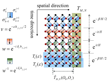
Figure 1: (Color online) Graphical representation of the evolution matrices $T_{1,2}(\varepsilon)$ and the quantum transfer matrix $T_{M,N}$. $\sigma_{k}^{j}$ is a basis state at site $j$ and time (or imaginary time) $k$. $\widetilde{T}_{M,N}(O_{0},O_{s})$ is a product of $s+1$ transfer matrices where the two empty circles represents two operators at different site and different time. Detailed definitions of these matrices are given in Supplementary Material S1.

We start from a 1D quantum system with $L$ sites and a Hamiltonian $H=\sum_{j=1}^{L}{h}_{j,j+1}$ with nearest-neighbor interactions and periodic boundary conditions. The time dependent correlation function for an operator $O$ between site $s$ and site $0$ at finite temperature can be expressed as

$$\left\langle O_{s}(t)O_{0}(0)\right\rangle=\frac{1}{Z}\text{Tr}\left(\text{e}^{-\beta H}\text{e}^{itH}O_{s}\text{e}^{-itH}O_{0}\right),$$ (1)

where $Z=\text{Tr(}$e${}^{-\beta H})$ is the partition function and $\beta=1/T$ is the inverse temperature.

We employ a quantum-to-classical mapping that decomposes the operator e^-βH into

$$\text{e}^{-\beta H}\approx\lim_{M\rightarrow\infty}\left[\emph{T}_{1}(\varepsilon)\emph{T}_{2}(\varepsilon)\right]^{M/2},$$ (2)

where $T_{1,2}(\varepsilon)=T_{R,L}$e^-εH is a row-to-row evolution operator, and $T_{R,L}$ are the right and left shift operators which are defined by the product of a 45^∘ clockwise and counter-clockwise rotated local operator $\nu\equiv$ e${}^{-\varepsilon h_{j,j+1}}$, respectively. $\varepsilon=\beta/M$ is the imaginary-time step and $M$ is the Trotter number in the imaginary-time direction Sirker and Klümper (2002). A similar decomposition can be applied to the operators e^-itH and e^itH by replacing $\nu$ with the complex local operators $w\equiv$ e${}^{-i\delta_{t}h_{j,j+1}}$ and $w^{-1}\equiv$ e${}^{i\delta_{t}h_{j,j+1}}$, respectively. Here $\delta_{t}=t/N$ and $N$ is the Trotter number in the time direction. From these decompositions a column-to-column QTM, $T_{M,N}$, can be defined. A graphical representation of $T_{M,N}$ is shown in Fig. 1 (a more detailed definition of $T_{M,N}$ is given in Supplementary Material S1).

In the thermodynamic limit, the correlation functions in Eq. (1) can be determined by the maximal eigenvalue $\Lambda_{0}$ and the corresponding left $\langle\psi_{M,N}^{l}|$ and right $|\psi_{M,N}^{r}\rangle$ eigenvectors of $T_{M,N}$:

$$\left\langle O_{s}(t)O_{0}(0)\right\rangle=\frac{\langle\psi_{M,N}^{l}|\widetilde{T}_{M,N}(O_{0},O_{s})\left|\psi_{M,N}^{r}\right\rangle}{\Lambda_{0}^{s+1}}.$$ (3)

Here $\langle\psi_{M,N}^{l}|\psi_{M,N}^{r}\rangle=1$ is implied and $\widetilde{T}_{M,N}(O_{0},O_{s})\equiv T_{M,N}(O_{0})T_{M,N}^{\text{ }s-1}T_{M,N}(O_{s})$ is a product of $s+1$ transfer matrices, where $T_{M,N}(O_{j})$ is a modified transfer matrix containing operator $O_{j}$ at site $j=0$ and $s$ (see Fig. 1).

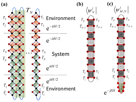
Figure 2: (Color online) (a) Graphical representation of the transfer matrix $T_{N}$. $\tau_{n}$ and $\overline{\tau}_{n}$ represent the time along the forward and backward evolution directions, respectively. (b) Schematic plot of the entanglement structure for the maximal left eigenvector of $T_{N}$. $\langle\psi_{N}^{l}|$ is an entangled state of singlet pairs between $\tau_{n}$ and $\overline{\tau}_{n}$. The two parts separated by a dark shadow has stronger entanglement than that separated by a light shadow. The right maximal eigenvector $|\psi_{N}^{r}\rangle$ has a similar entanglement structure with the dark and light shadows interchanged. The new TMRG scheme bi-partitions the QTM into e^itH/2e^-itH/2 and e^-itH/2e^itH/2 such that the maximally entangled pair is locked within each block. (c) The maximal eigenvectors of $T_{M,N}$ at finite temperature have similar structures.

In order to evaluate the long time correlation function accurately, one needs to understand how the entanglement is built up in the maximal eigenvectors of $T_{M,N}$ during the time evolution. It is instructive to first consider the infinite-temperature case where the thermal density matrix e^-βH becomes an identity and $T_{M,N}$ associated with its dual eigenvectors $\langle\psi_{M,N}^{l}|$ and $|\psi_{M,N}^{r}\rangle$ are reduced to an $M$-independent matrix $T_{N}$ associated with $\langle\psi_{N}^{l}|$ and $|\psi_{N}^{r}\rangle$ (Fig. 2(a)). For the convenience in the discussion below, we use $\tau_{n}^{\ast}$ to denote a pair of virtual states $(\tau_{n},\overline{\tau}_{n})$, $n=1,...N,$ and $|\tau_{n}^{\ast}\rangle=\sum_{\tau_{n}\overline{\tau}_{n}}\delta_{\tau_{n},\overline{\tau}_{n}}|\tau_{n},\overline{\tau}_{n}\rangle$ to denote a maximally entangled state of $\tau_{n}$ and $\overline{\tau}_{n}$. An important property of $T_{n}$, as shown in the supplementary material, is that the contraction of its left maximal eigenvector $\langle\psi_{n}^{l}|$ with $|\tau_{n}^{\ast}\rangle$ satisfies the following equation

$$\langle\psi_{n}^{l}|\tau_{n}^{\ast}\rangle=\langle\psi_{n-1}^{l}|=\langle\psi_{n-2}^{l}|\langle\tau_{n-1}^{\ast}|$$ (4)

for an even $n$. A similar equation holds for the right eigenvector $|\psi_{n}^{r}\rangle$ but with odd $n$. Eq. 4 means that the contraction of the left eigenvector $\langle\psi_{n}^{l}|$ with a maximally entangled pair $|\tau_{n}^{\ast}\rangle$ produces another separated maximally entangled pair $|\tau_{n-1}^{\ast}\rangle$ if $n$ is even. This implies that the virtual basis states $\tau_{n}$ and $\overline{\tau}_{n}$ at the same forward and backward real time $n$ have strong tendency to form a singlet pair. Thus the left maximal eigenvector should have an entanglement structure as depicted in Fig. 2(b), where the red bonds denote singlet pair states, and the upper and lower parts separated by a dark (light) shadow have stronger (weaker) entanglement. A similar entanglement structure exists for the right maximal eigenvector $|\psi_{n}^{r}\rangle$, but the dark and light shadows are interchanged.

As taking into account the finite temperature effect, the QTM $T_{M,N}$ is obtained by simply adding two blocks of thermal operator at the top and bottom of $T_{N}$ as shown in Fig. 1. Following the derivation of Eq. (4) (see Supplementary Material S2), we can obtain

$$\langle\psi_{M,n}^{l}|\tau_{n}^{\ast}\rangle=\langle\psi_{M,n-1}^{l}|=\langle\psi_{M,n-2}^{l}|\langle\tau_{n-1}^{\ast}|$$ (5)

for an even real-time $n$, and the eigenvector $|\psi_{M,n}^{r}\rangle$ has a similar property for odd $n$. Here $\langle\psi_{M,n}^{l}|$ and $|\psi_{M,n}^{r}\rangle$ denote the left and right maximal eigenvectors of $T_{M,n}$ with $M$ fixed and $n=1,...,N$. Thus, the eigenvectors of $T_{M,N}$ should have a slower increasing entanglement between the block involving imaginary-time and the block involving real-time. Furthermore, the eigenvectors of $T_{M,N}$ should have a similar entanglement structure for the block involving real-time as the structure of the eigenvectors of $T_{N}$ (see Fig. 2(c)).

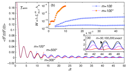
Figure 3: (Color online) Time-dependent autocorrelation $\langle S^{z}(t)S^{z}(0)\rangle$ for the Heisenberg model (6) with $\Delta=0$ at infinite temperature. $m$ is the number of basis states retained in the calculation. The results The data with $m$ marked by asterisk are obtained by the conventional TMRG scheme. Inset (a): Blow-up of the autocorrelation in the long time region. Inset (b): Comparison of the discarded weight $W=1-\sum_{k=1}^{m}\Lambda_{k}$ obtained by the BTMRG with that obtained by the conventional TMRG. The two $W$-curves for our scheme correspond to the cutting boundary through the dark shadow with strong entanglement and through the light shadow with weak entanglement, respectively.

The above discussion suggests that in order to suppress the growth of the entanglement with time evolution, we should redefine $T_{N}$ on a folded lattice where $\tau_{n}$ and $\overline{\tau}_{n}$ at real time $n$ are merged into a single site, as shown in Fig. 2(b). For $T_{M,N}$ on a folded lattice, the additional sites $\tau_{m}$ and $\overline{\tau}_{m}$ for imaginary time are also merged, but the folded block e^-βH is regarded as a heat bath (Fig. 2(c)). Thus the strong entanglement between $\tau_{N}$ and $\overline{\tau}_{N}$ is confined within each time step and will not proliferate with time evolution. This can avoid the linear growth problem of entanglement with time in the conventional TMRG schemesSirker and Klümper (2005).

Based on the above argument, we propose to do the BTMRG calculation by collecting a segment of local matrices around the center of the virtual lattice as the system block and the rest of local tensors as the environment block (Fig. 2(a)). In the infinite temperature limit, this is equivalent to dividing the quantum transfer matrix into $e^{itH/2}e^{-itH/2}$ and $e^{-itH/2}e^{itH/2}$ parts. At each iteration, both system and environment blocks are enlarged by adding two different rotated matrices $w^{,}s$ ($w^{-1,}s$) at the upper (lower) boundary site between the two blocks. For the finite-temperature calculation, we first cool down the temperature to a desired value by taking the imaginary time evolution, and then take the real time evolution by embedding $T_{M}$ into the environment block. in this case, the system and environment blocks are equivalent to $e^{itH/2}e^{-itH/2}$ and $e^{-itH/2}e^{-\beta H}e^{itH/2}$, respectively.

To test the method, we calculate the longitudinal spin autocorrelation $\langle S^{z}(t)S^{z}(0)\rangle$ for the anisotropic spin-1/2 Heisenberg model defined by the Hamiltonian

$$H=\sum_{j}J(S_{j}^{x}S_{j+1}^{x}+S_{j}^{y}S_{j+1}^{y}+\Delta S_{j}^{z}S_{j+1}^{z}).$$ (6)

When $\Delta=0$, this model is equivalent to the spinless free fermion model where an exact result for the autocorrelation is available Nie . We use the BTMRG to evaluate the maximal eigenvectors of $T_{M,N}$ Huang (2011a); *YHuang2011b. By properly choosing the dual biorthonormal bases, the BTMRG can achieve significant improvement of numerical stability over the conventional TMRG.

Fig. 3 compares the results of the autocorrelation for the above above model up to $Jt=50$ with $\delta_{t}=0.05$ and $\Delta=0$ at infinite temperature obtained from both the BTMRG and the conventional TMRG. We find that the time scale that can be reached by the conventional TMRG with reliable accuracy is quite small, due to the fast increase of entanglement entropy with evolving time. However, our BTMRG calculation can reach much longer time scale with high precision. In particular, as shown in Fig. 3(b) the truncation error $W=1-\sum_{k=1}^{m}\Lambda_{k}$ increases very rapidly with increasing time scale in the TMRG calculation. In contrast, in our BTMRG calculation $W$ saturates asymptotically. This shows that the entanglement builds up mainly between the operators e^-itH and e^itH. We also calculate the real-time dynamics for several spin-1/2 chains at various temperatures. The results are consistent with our prediction for the entanglement structure at finite temperature and the dynamics can be reliably evaluated on a time scale far longer than the previous TMRG calculations (see the supplementary material).

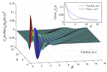
Figure 4: (Color online) The correlation function $C_{s}(t)$ for the Heisenberg model with $\Delta=1$ and $s=0-15$ at $T/J=0.5$. Inset: Current correlation function $C(t)$ for $\Delta=1$ at $T/J=0.5$ and $T=\infty$, respectively.

An advantage of our BTMRG scheme is its competitive accuracy with much cheaper computational cost. The computational cost of the BTMRG scales with the basis states retained as $O(m^{3})$, one order less than in the folding algorithm as well as the tDMRG using matrix product states where the computational cost scales as $O(m^{4})$. Moreover, our method works directly in the thermodynamic limit and there is no finite lattice size effect. The most challenging problem in our method is the calculation of long distance correlation functions, since it involves a calculation of the product of many transfer matrices $\widetilde{T}_{M,N}(O_{0},O_{s})$ (see Fig. 1).

In our algorithm, this wide transfer matrix $\widetilde{T}_{M,N}(O_{0},O_{s})$ is approximated by a matrix-product operator (MPO) and is updated in a similar way as the evolution of the matrix product state in the modified tDMRGKarrasch et al. (2012); *Barthel2012 (see the supplementary material). Our method, however, differs from the modified tDMRG in three aspects: (i) The infinite-length MPO used in tDMRG for the correlator is replaced by a $(s+1)$-length MPO representing the transfer matrix $\widetilde{T}_{M,N}(O_{0},O_{s})$. This leads to dramatic reduction of computational storage and time. (ii) The left (right) bond of the first (last) MPO matrix is obtained by projecting the matrix from the left (right) onto the reduced basis states describing the left (right) maximal eigenvector. Since the number of state kept, $m$, is usually small due to our special bi-partitioning scheme, the bond dimension $\chi$ of the MPO matrices is typically smaller than that in tDMRG. (iii) The correlator is obtained by contracting the $(s+1)$-length MPO with the left and right maximal eigenvectors at the left and right bonds respectively. These advantages can be seen from the calculation of the current-current correlation functionKarrasch et al. (2012); Sirker et al. (2009); *Sirker:2011ST; *Jesenko2011

$$C_{s}(t)=\langle j_{s}(t)j_{0}(0)\rangle,$$ (7)

where $j_{s}=-\frac{iJ}{2}(S_{s}^{+}S_{s+1}^{-}-S_{s+1}^{+}S_{s}^{-})$. The long time limit of $C(t)=\sum_{s}C_{s}(t)$ gives the value of Drude weight. Fig. 4 shows $C_{s}(t)$ for the Heisenberg model (6) with $\Delta=1$ and $s=0-15$ at $T/J=0.5$. The result is obtained by fixing the truncation error less than $W=1\times 10^{-11}$ for the maximal eigenvectors (the number of basis states is typically around $m=250$) and less than $W=1\times 10^{-6}$ for the evolution of matrix product operators with the bond dimension around $\chi=500$. The figure clearly shows that the large distance and long-time dynamics can be accurately determined. Another notable advantage of our method is that in the determination of these correlation functions, the left and right maximal eigenvectors need to be evaluated just once. The inset of Fig. 4 shows the spatial integrated current correlation function $C(t)$ up to time scale where $C(t)$ saturates for $\Delta=1$ at $T/J=0.5$ and $T=\infty$, which agree well with the results given in Refs. Karrasch et al., 2012; Sirker et al., 2009.

To summarize, we identify the entanglement structure of the maximal eigenvectors of the QTM proposed in Sirker and Klümper (2002). It reveals the origin of the entanglement growth during the time evolution and the reason why the recent algorithms work Bañuls et al. (2009); Karrasch et al. (2012). On the basis of this picture, we propose an alternative method based on the BTMRG approach by bi-partitioning the system and the environment blocks according to the entanglement structure. Our approach provides an very efficient tool for studying finite-temperature dynamics of 1D quantum lattice models.