High temperature superconductivity in the two-dimensional $t$-$J$ model: Gutzwiller wave function solution

Abstract

A systematic diagrammatic expansion for Gutzwiller-wave functions (DE-GWF) proposed very recently is used for the description of superconducting (SC) ground state in the two-dimensional square-lattice $t$-$J$ model with the hopping electron amplitudes $t$ (and $t^{\prime}$) between nearest (and next-nearest) neighbors. On the example of the SC state analysis we provide a detailed comparison of the method results with other approaches. Namely: (i) the truncated DE-GWF method reproduces the variational Monte Carlo (VMC) results; (ii) in the lowest (zeroth) order of the expansion the method can reproduce the analytical results of the standard Gutzwiller approximation (GA), as well as of the recently proposed “grand-canonical Gutzwiller approximation” (GCGA). We obtain important features of the SC state. First, the SC gap at the Fermi surface resembles a $d_{x^{2}-y^{2}}$-wave only for optimally- and overdoped system, being diminished in the antinodal regions for the underdoped case in a qualitative agreement with experiment. Corrections to the gap structure are shown to arise from the longer range of the real-space pairing. Second, the nodal Fermi velocity is almost constant as a function of doping and agrees semi-quantitatively with experimental results. Third, we compare the doping dependence of the gap magnitude with experimental data. Fourth, we analyze the $\mathbf{k}$-space properties of the model: Fermi surface topology and effective dispersion. The DE-GWF method opens up new perspectives for studying strongly-correlated systems, as: (i) it works in the thermodynamic limit, (ii) is comparable in accuracy to VMC, and (iii) has numerical complexity comparable to GA (i.e., it provides the results much faster than the VMC approach).

I Introduction

The Hubbard and the $t$-$J$ models of strongly correlated fermions play an eminent role in rationalizing the principal properties of high temperature superconductors (for recent reviews see Lee et al. (2006); Ogata and Fukuyama (2008); Scalapino (2012); Edegger et al. (2007); Anderson (2007)). The relative role of the particles’ correlated motion and the binding provided by the kinetic exchange interaction can be clearly visualized in the effective $t$-$J$ model, where the effective hopping energy $\sim|t|\delta\sim 0.35\,\rm{eV}$ ($\delta\equiv 1-2n$ is the hole doping) is comparable or even lower than the kinetic exchange integral $J\approx 0.12\,\rm{eV}$. Simply put, the hopping electron drags behind its exchange-coupled nearest neighbor (n.n.) via empty sites and thus preserves the locally bound configuration in such correlated motion throughout the lattice Spałek and Goc-Jagło (2012). In effect, this real-space pairing picture is complementary to the more standard virtual boson (paramagnon) exchange mechanism which involves, explicitly or implicitly, a quasiparticle picture and concomitant with it reciprocal-space language Maier et al. (2006a); *PhysRevB.74.094513; Monthoux et al. (1991); Kyung et al. (2009); Hanke et al. (2010). Unfortunately, no single unifying approach, if possible at all, exists in the literature which would unify the Eliashberg-type and the real-space approaches, out of which a Cooper-pair condensate would emerge as a universal state for arbitrary ratio of the band energy $\sim W$ to the Coulomb repulsion $U$. The reason for this exclusive character of the approaches is ascribed to the presence of the Mott-Hubbard phase transition that takes place for $W/U\approx 1$ (appearing for the half-filled band case) which also delineates the strong-correlation limit for a doped-Mott metallic state, for $W$ substantially smaller than $U$. This is the regime, where the $t$-$J$ model is assumed to be valid, even in the presence of partially-filled oxygen $2p$ states Hanke et al. (2010); Anderson (1988); Zhang and Rice (1988); *PhysRevB.41.7243; Spałek (1988a); *Spalek2. The validity of this type of physics is assumed throughout the present paper and a quantitative analysis of selected experimental properties, as well as a comparison with variational Monte-Carlo (VMC) results, is undertaken.

One of the approaches designed to interpolate between the $W/U\gg 1$ and $W/U\lesssim 1$ limits is the Gutzwiller wave function (GWF) approach Gutzwiller (1963); *PhysRev.137.A1726. Unfortunately, the method does not allow for an extrapolation to the $W/U\ll 1$ limit, at least in the simpler Gutzwiller approximation (GA) Zhang et al. (1988). Therefore, different forms of the GA-like approaches, appropriate for the $t$-$J$ model, have been invented under the name of the Renormalized Mean Field Theory (RMFT) Zhang et al. (1988); Ogata and Himeda (2003); Wang et al. (2006); Fukushima (2008, 2011); Jȩdrak and Spałek (2011); Edegger et al. (2007). The last approach based on the $t$-$J$ model provides a rationalization of the principal characteristics of high temperature superconductors, including selected properties in a semiquantitative manner, particularly when the so-called statistically consistent Gutzwiller approach (SGA) Jȩdrak and Spałek (2010, 2011); Kaczmarczyk and Spałek (2011); Howczak et al. (2013); Zegrodnik et al. (2013); Abram et al. (2013) is incorporated into RMFT. However, one should also mention that neither GA nor SGA provide a stable superconducting state in the Hubbard model.

Under these circumstances, we have undertaken a project involving a full GWF solution via a systematic Diagrammatic Expansion of the GWF (DE-GWF), which becomes applicable to two- and higher-dimensional systems, for both normalBünemann et al. (2012) and superconductingKaczmarczyk et al. (2013) states. Previously, this solution has been achieved in one-spatial dimension in an iterative manner Metzner and Vollhardt (1988); Kurzyk et al. (2007). Obviously, the DE-GWF should reduce to SGA in the limit of infinite dimensions. In our preceding paperKaczmarczyk et al. (2013) we have presented the first results for the Hubbard model. Here, a detailed analysis is provided for the $t$-$J$ model, together with a comparison to experiment, as well as to the VMC and GA results. The limitations of the present approach are also discussed, particularly the inability to describe the pseudogap appearance.

The structure of the paper is as follows. In Sec. II we present the DE-GWF method (cf. also Appendices A and B). In Secs. III and IV (cf. also Appendices C, D, and E) we provide details of the numerical analysis and discuss physical results, respectively. In the latter section, we also compare our results with experiment and relate them to VMC and GA results. Finally, in Sec. V we draw conclusions and overview our approach.

II The method

II.1 $t$-$J$ Model

We start with the $t$-$J$ model Hamiltonian on a two-dimensional, infinite square lattice

$$\hat{H} = \hat{H}_{0}+\hat{H}_{ex}\,,$$ (1)

$$\hat{H}_{0} = \sum_{{\bf i},{\bf j},\sigma}t_{{\bf i}{\bf j}}\hat{c}_{{\bf i},\sigma}^{\dagger}(1-\hat{n}_{{\bf i}\overline{\sigma}})\hat{c}_{{\bf j},\sigma}^{\phantom{\dagger}}(1-\hat{n}_{{\bf j}\overline{\sigma}}),$$ (2)

$$\hat{H}_{ex} = J\sum_{\langle{\bf i},{\bf j}\rangle}\left(\mathbf{\hat{S}_{\bf i}}\mathbf{\hat{S}_{\bf j}}-c\frac{1}{4}\hat{\nu}_{\bf i}\hat{\nu}_{\bf j}\right),$$ (3)

where $\hat{\nu}_{\bf i}=\hat{\nu}_{{\bf i}\uparrow}+\hat{\nu}_{{\bf i}\downarrow}$ with $\hat{\nu}_{{\bf i}\sigma}\equiv\hat{n}_{{\bf i}\sigma}(1-\hat{n}_{{\bf i}\overline{\sigma}})$, the first term is the kinetic energy part and the second expresses the kinetic exchange. The spin operator is defined as $\mathbf{\hat{S}_{\bf i}}=\{\hat{S}_{\bf i}^{z},\hat{S}_{\bf i}^{+},\hat{S}_{\bf i}^{-}\}$ and $\sum_{\langle{\bf i},{\bf j}\rangle}$ denotes summation over pairs of n.n. sites (bonds). The parameter $c$ is used to switch on ($c=1$) or off ($c=0$) the density-density interaction term reproducing the two forms of the model used in the literature. Unless stated otherwise, the system’s spin-isotropy and the translational invariance are not assumed and the analytical results presented in this section are valid for phases with broken symmetries. We study system properties in the thermodynamic limit, i.e., the system size $L$ is infinite. We also neglect the three-site terms.

II.2 Trial wave function

The principal task within a Gutzwiller-typeGutzwiller (1963) of approach is the calculation of the expectation value of the starting Hamiltonian with respect to the trial wave function, which is defined as

$$|\Psi_{\rm G}\rangle=\hat{P}|\Psi_{0}\rangle\equiv\prod\nolimits_{{\bf i}}\hat{P}_{{\bf i}}|\Psi_{0}\rangle\;,$$ (4)

where $|\Psi_{0}\rangle$ is a single-particle product state (Slater determinant) to be specified later. We define the local Gutzwiller correlator in the atomic basis of the form

$$\hat{P}_{{\bf i}}\equiv\sum_{\Gamma}\lambda_{{\bf i},\Gamma}|\Gamma\rangle_{{\bf i}\,{\bf i}}\!\langle\Gamma|\;,$$ (5)

with variational parameters $\lambda_{{\bf i},\Gamma}\in\left\{\lambda_{{\bf i},\emptyset},\lambda_{{\bf i},1\uparrow},\lambda_{{\bf i},1\downarrow},\lambda_{{\bf i},d}\right\}$, which describe the occupation probabilities of the four possible local states $\{|\Gamma\rangle_{{\bf i}}\}\equiv\left\{|\emptyset\rangle_{{\bf i}},|\uparrow\rangle_{{\bf i}},|\downarrow\rangle_{{\bf i}},|\uparrow\downarrow\rangle_{{\bf i}}\right\}$. A particularly useful choice of the parameters $\lambda_{{\bf i},\Gamma}$ is the one which obeys

$$\hat{P}^{2}_{{\bf i}}\equiv 1+x\hat{d}_{{\bf i}}^{\rm HF}\;,$$ (6)

where the Hartree–Fock operators are defined by $\hat{d}_{{\bf i}}^{\rm HF}\equiv\hat{n}^{\rm HF}_{{\bf i}\uparrow}\hat{n}^{\rm HF}_{{\bf i}\downarrow}$ and $\hat{n}^{\rm HF}_{{\bf i}\sigma}\equiv\hat{n}_{{\bf i},\sigma}-n_{{\bf i}\sigma}$ with $n_{{\bf i}\sigma}=\langle\Psi_{0}|\hat{n}_{{\bf i}\sigma}|\Psi_{0}\rangle$. This form of $\hat{P}^{2}_{{\bf i}}$ decisively simplifies the calculations by eliminating the so-called ‘Hartree bubbles’ Gebhard (1990); Bünemann et al. (2012).

For the t-J model, we work with zero double-occupancy, which sets $\lambda_{{\bf i},d}=0$ and eliminates $x$ as a variational parameter from the solution procedure. Explicitly, from the conditions in Eqs. (5) and (6) we find $\lambda_{{\bf i},d}^{2}=1+x(1-n_{{\bf i}\uparrow})(1-n_{{\bf i}\downarrow})=0$. Calculating $x$ and inserting to the expressions for $\lambda_{{\bf i},1\sigma}$ and $\lambda_{{\bf i},\emptyset}$ gives

$$\lambda_{{\bf i},1\sigma} = \frac{1}{\sqrt{1-n_{{\bf i}\overline{\sigma}}}},$$ (7)

$$\lambda_{{\bf i},\emptyset} = \sqrt{\frac{1-n_{\bf i}}{(1-n_{{\bf i}\sigma})(1-n_{{\bf i}\overline{\sigma}})}},$$ (8)

where $n_{\bf i}=n_{{\bf i}\uparrow}+n_{{\bf i}\downarrow}$.

II.3 Diagrammatic sums

Here we discuss the analytical procedure of calculating the expectation value

$$W\equiv\langle\hat{H}\rangle_{\rm G}\equiv\frac{\langle\Psi_{\rm G}|\hat{H}|\Psi_{\rm G}\rangle}{\langle\Psi_{\rm G}|\Psi_{\rm G}\rangle}\equiv\frac{\langle\Psi_{0}|\hat{P}\hat{H}\hat{P}|\Psi_{0}\rangle}{\langle\Psi_{0}|\hat{P}^{2}|\Psi_{0}\rangle}$$ (9)

in detail for the kinetic-energy term and we summarize the results for other terms. We start with expressions for the relevant expectation values of interest via the power series in $x$, i.e.,

$$\langle\Psi_{\rm G}|\Psi_{\rm G}\rangle=\Bigl{\langle}\prod_{{\bf l}}\hat{P}^{2}_{{\bf l}}\Bigr{\rangle}_{0} = \sum_{k=0}^{\infty}\frac{x^{k}}{k!}\sideset{}{{}^{\prime}}{\sum}_{{\bf l}_{1},\ldots,{\bf l}_{k}}\bigl{\langle}\hat{d}^{\rm HF}_{{\bf l}_{1},\ldots,{\bf l}_{k}}\bigr{\rangle}_{0}\,,$$ (10)

$$\langle\Psi_{\rm G}|\hat{c}^{\dagger}_{{\bf i},\sigma}\hat{c}_{{\bf j},\sigma}^{\phantom{\dagger}}|\Psi_{\rm G}\rangle=\Bigl{\langle}\widetilde{c}^{\dagger}_{{\bf i},\sigma}\widetilde{c}_{{\bf j},\sigma}^{\phantom{\dagger}}\prod_{{\bf l}(\neq{\bf i},{\bf j})}\hat{P}^{2}_{{\bf l}}\Bigr{\rangle}_{0} = \sum_{k=0}^{\infty}\frac{x^{k}}{k!}\sideset{}{{}^{\prime}}{\sum}_{{\bf l}_{1},\ldots,{\bf l}_{k}}\bigl{\langle}\widetilde{c}_{{\bf i},\sigma}^{\dagger}\widetilde{c}_{{\bf j},\sigma}^{\phantom{\dagger}}\hat{d}^{\rm HF}_{{\bf l}_{1},\ldots,{\bf l}_{k}}\bigr{\rangle}_{0}\,,$$ (11)

where $\langle(...)\rangle_{0}\equiv\langle\Psi_{0}|(...)|\Psi_{0}\rangle$, $\widetilde{c}_{{\bf i},\sigma}^{(\dagger)}\equiv\hat{P}_{{\bf i}}\hat{c}_{{\bf i},\sigma}^{(\dagger)}\hat{P}_{{\bf i}}$, and we have defined $\hat{d}^{\rm HF}_{{\bf l}_{1},\ldots,{\bf l}_{k}}\equiv\hat{d}^{\rm HF}_{{\bf l}_{1}}\cdots\hat{d}^{\rm HF}_{{\bf l}_{k}}$ with $\hat{d}^{\rm HF}_{\emptyset}\equiv 1$, whereas the primed sums have the summation restrictions ${\bf l}_{p}\neq{\bf l}_{p^{\prime}}$, ${\bf l}_{p}\neq{\bf i},{\bf j}$ for all $p,p^{\prime}$.

Expectation values can now be evaluated by means of the Wick’s theorem Fetter and Walecka (2003) and are carried out in real space. Then, in the resulting diagrammatic expansion, the $k$-th order terms of Eqs. (10)-(11) correspond to diagrams with one (or two) external vertices on sites ${\bf i}$ (or ${\bf i}$ and ${\bf j}$) and $k$ internal vertices. These vertices are connected with lines (corresponding to contractions from Wick’s theorem), which in the case of the superconducting state with intersite pairing are given by

$$P_{{\bf l},{\bf l}^{\prime}}\equiv P^{\sigma}_{{\bf l},{\bf l}^{\prime}}\equiv\langle\hat{c}^{\dagger}_{{\bf l},\sigma}\hat{c}_{{\bf l}^{\prime},\sigma}^{\phantom{\dagger}}\rangle_{0}-\delta_{{\bf l},{\bf l}^{\prime}}n\;,\qquad S_{{\bf l},{\bf l}^{\prime}}\equiv\langle\hat{c}^{\dagger}_{{\bf l},\uparrow}\hat{c}^{\dagger}_{{\bf l}^{\prime},\downarrow}\rangle_{0},$$ (12)

where $\bar{\uparrow}=\downarrow$, $\bar{\downarrow}=\uparrow$. At this point, the application of the linked-cluster theorem Fetter and Walecka (2003) yields Bünemann et al. (2012) the analytical result for the kinetic energy term

$$\langle\hat{H}_{0}\rangle_{\rm G}=\sum_{{\bf i},{\bf j},\sigma}t_{{\bf i},{\bf j}}\left(q_{{\bf i}\sigma}q_{{\bf j}\sigma}T_{{\bf i},{\bf j},\sigma}^{(1),(1)}+q_{{\bf i}\sigma}\alpha_{{\bf j}\sigma}T_{{\bf i},{\bf j},\sigma}^{(1),(3)}+\alpha_{{\bf i}\sigma}q_{{\bf j}\sigma}T_{{\bf i},{\bf j},\sigma}^{(3),(1)}+\alpha_{{\bf i}\sigma}\alpha_{{\bf j}\sigma}T_{{\bf i},{\bf j},\sigma}^{(3),(3)}\right),$$ (13)

where

$$q_{{\bf i}\sigma} \equiv \lambda_{{\bf i},1\sigma}\lambda_{{\bf i},\emptyset}(1-n_{\bf i})=\sqrt{\frac{1-n_{\bf i}}{1-n_{{\bf i},\sigma}}},$$ (14)

$$\alpha_{{\bf i}\sigma} \equiv -\lambda_{{\bf i},1\sigma}\lambda_{{\bf i},\emptyset}=-\frac{1}{1-n_{{\bf i}\overline{\sigma}}}\sqrt{\frac{1-n_{\bf i}}{1-n_{{\bf i},\sigma}}}=-\frac{q_{{\bf i}\sigma}}{1-n_{{\bf i}\overline{\sigma}}}.$$ (15)

The diagrammatic sums appearing in Eq. (13) are defined by

$$S=\sum_{k=0}^{\infty}\frac{x^{k}}{k!}S(k),$$ (16)

where

$$S\in\left\{T_{{\bf i},{\bf j},\sigma}^{(1),(1)},T_{{\bf i},{\bf j},\sigma}^{(1),(3)},T_{{\bf i},{\bf j},\sigma}^{(3),(1)},T_{{\bf i},{\bf j},\sigma}^{(3),(3)}\right\}$$ (17)

and the $k$-th order sum contributions have the following forms

$$T_{{\bf i},{\bf j},\sigma}^{(1)[(3)],(1)[(3)]}(k)\equiv\sum_{{\bf l}_{1},\ldots,{\bf l}_{k}}\bigl{\langle}[\hat{n}^{\rm HF}_{{\bf i},\bar{\sigma}}]\hat{c}^{\dagger}_{{\bf i},\sigma}[\hat{n}^{\rm HF}_{{\bf j},\bar{\sigma}}]\hat{c}_{{\bf j},\sigma}^{\phantom{\dagger}}\hat{d}^{\rm HF}_{{\bf l}_{1},\ldots,{\bf l}_{k}}\bigr{\rangle}^{\rm c}_{0}$$ (18)

where $\langle\dots\rangle_{0}^{\rm c}$ indicates that only the connected diagrams are to be kept (see Appendix A for exemplary diagrams and their contributions to diagrammatic sums in the two lowest orders). The notation $(1)[(3)]$ means that for the index (3) also the term in square brackets needs to be taken into account, e.g. $T_{{\bf i},{\bf j},\sigma}^{(1),(3)}(k)\equiv\sum_{{\bf l}_{1},\ldots,{\bf l}_{k}}\bigl{\langle}\hat{c}^{\dagger}_{{\bf i},\sigma}\hat{n}^{\rm HF}_{{\bf j},\bar{\sigma}}\hat{c}_{{\bf j},\sigma}^{\phantom{\dagger}}\hat{d}^{\rm HF}_{{\bf l}_{1},\ldots,{\bf l}_{k}}\rangle^{\rm c}_{0}$. In the following expressions we will drop the brackets in the upper indices of diagrammatic sums for the sake of brevity.

The exchange term can be rewritten in the form

$$J\sum_{\langle{\bf i},{\bf j}\rangle}\left(\mathbf{\hat{S}_{\bf i}}\mathbf{\hat{S}_{\bf j}}-\frac{1}{4}\hat{\nu}_{\bf i}\hat{\nu}_{\bf j}\right)=J\sum_{\langle{\bf i},{\bf j}\rangle}\left(\frac{\hat{S}_{\bf i}^{+}\hat{S}_{\bf j}^{-}+\hat{S}_{\bf i}^{-}\hat{S}_{\bf j}^{+}}{2}+\hat{S}_{\bf i}^{z}\hat{S}_{\bf j}^{z}-\frac{1}{4}\hat{\nu}_{\bf i}\hat{\nu}_{\bf j}\right),$$ (19)

where the spin-component operators are given by $\{\hat{S}_{\bf i}^{+},\hat{S}_{\bf i}^{-},\hat{S}_{\bf i}^{z}\}=\{\hat{c}^{\dagger}_{{\bf i}\uparrow}\hat{c}_{{\bf i}\downarrow},\hat{c}^{\dagger}_{{\bf i}\downarrow}\hat{c}_{{\bf i}\uparrow},\frac{1}{2}(\hat{n}_{{\bf i}\uparrow}-\hat{n}_{{\bf i}\downarrow})\}$. The expectation values of the exchange term components can be expressed as

$$\frac{1}{2}\langle\hat{S}_{\bf i}^{+}\hat{S}_{\bf j}^{-}+\hat{S}_{\bf i}^{-}\hat{S}_{\bf j}^{+}\rangle_{G}=\left[(n_{{{\bf i}\downarrow}}-1)(n_{{{\bf i}\uparrow}}-1)(n_{{{\bf j}\downarrow}}-1)(n_{{{\bf j}\uparrow}}-1)\right]^{-1/2}\frac{S_{{\bf i}\uparrow,{\bf j}\downarrow}^{22}+S_{{\bf i}\downarrow,{\bf j}\uparrow}^{22}}{2}.$$ (20)

For the expressions of the other components see Appendix B.

The diagrammatic sums appearing in the above expressions are defined by Eq. (16) with

$$S\in\left\{I_{{\bf i}[{\bf j}]\sigma}^{2},I_{{\bf i}[{\bf j}]}^{4},I_{{\bf i}\sigma,{\bf j}\sigma^{\prime}}^{22},I_{{\bf i}\sigma,{\bf j}}^{24},I_{{\bf i},{\bf j}\sigma}^{42},I_{{\bf i},{\bf j}}^{44},S_{{\bf i}\sigma,{\bf j}\overline{\sigma}}^{22}\right\}$$ (21)

and the $k$-th order sum contributions of the following forms

$$I_{{\bf i}[{\bf j}]\sigma}^{2}(k) \equiv \sum_{{\bf l}_{1},\ldots,{\bf l}_{k}}\bigl{\langle}\hat{n}^{\rm HF}_{{\bf i}[{\bf j}]\sigma}\hat{d}^{\rm HF}_{{\bf l}_{1},\ldots,{\bf l}_{k}}\bigr{\rangle}^{\rm c}_{0},$$ (22)

$$I_{{\bf i}[{\bf j}]}^{4}(k) \equiv \sum_{{\bf l}_{1},\ldots,{\bf l}_{k}}\bigl{\langle}\hat{d}^{\rm HF}_{{\bf i}[{\bf j}]}\hat{d}^{\rm HF}_{{\bf l}_{1},\ldots,{\bf l}_{k}}\bigr{\rangle}^{\rm c}_{0},$$ (23)

$$I_{{\bf i}\sigma,{\bf j}\sigma^{\prime}}^{22}(k) \equiv \sum_{{\bf l}_{1},\ldots,{\bf l}_{k}}\bigl{\langle}\hat{n}^{\rm HF}_{{\bf i}\sigma}\hat{n}^{\rm HF}_{{\bf j}\sigma^{\prime}}\hat{d}^{\rm HF}_{{\bf l}_{1},\ldots,{\bf l}_{k}}\bigr{\rangle}^{\rm c}_{0},$$ (24)

$$I_{{\bf i}\sigma,{\bf j}}^{24}(k) \equiv \sum_{{\bf l}_{1},\ldots,{\bf l}_{k}}\bigl{\langle}\hat{n}^{\rm HF}_{{\bf i}\sigma}\hat{d}^{\rm HF}_{{\bf j}}\hat{d}^{\rm HF}_{{\bf l}_{1},\ldots,{\bf l}_{k}}\bigr{\rangle}^{\rm c}_{0},$$ (25)

$$I_{{\bf i},{\bf j}\sigma}^{42}(k) \equiv \sum_{{\bf l}_{1},\ldots,{\bf l}_{k}}\bigl{\langle}\hat{d}^{\rm HF}_{{\bf i}}\hat{n}^{\rm HF}_{{\bf j}\sigma}\hat{d}^{\rm HF}_{{\bf l}_{1},\ldots,{\bf l}_{k}}\bigr{\rangle}^{\rm c}_{0},$$ (26)

$$I_{{\bf i},{\bf j}}^{44}(k) \equiv \sum_{{\bf l}_{1},\ldots,{\bf l}_{k}}\bigl{\langle}\hat{d}^{\rm HF}_{{\bf i}}\hat{d}^{\rm HF}_{{\bf j}}\hat{d}^{\rm HF}_{{\bf l}_{1},\ldots,{\bf l}_{k}}\bigr{\rangle}^{\rm c}_{0},$$ (27)

$$S_{{\bf i}\sigma,{\bf j}\overline{\sigma}}^{22}(k) \equiv \sum_{{\bf l}_{1},\ldots,{\bf l}_{k}}\bigl{\langle}\hat{c}^{\dagger}_{{\bf i}\sigma}\hat{c}_{{\bf i}\overline{\sigma}}\hat{c}^{\dagger}_{{\bf j}\overline{\sigma}}\hat{c}_{{\bf j}\sigma}\hat{d}^{\rm HF}_{{\bf l}_{1},\ldots,{\bf l}_{k}}\bigr{\rangle}^{\rm c}_{0}.$$ (28)

In what follows, we evaluate these diagrammatic sums in particular situations.

II.4 Spin-isotropic case

The above expressions simplify significantly when a system with translational invariance and spin isotropy is considered. Explicitly, they become

$$\langle\hat{c}^{\dagger}_{{\bf i},\sigma}\hat{c}_{{\bf j},\sigma}\rangle_{G} = q^{2}T^{11}+2q\alpha T^{13}+\alpha^{2}T^{33},$$ (29)

$$\frac{1}{2}\langle\hat{S}_{\bf i}^{+}\hat{S}_{\bf j}^{-}+\hat{S}_{\bf i}^{-}\hat{S}_{\bf j}^{+}\rangle_{G} = g_{s}S^{22},$$ (30)

$$\langle\hat{S}_{\bf i}^{z}\hat{S}_{\bf j}^{z}\rangle_{G} = g_{s}\left(\frac{I^{22\uparrow\uparrow}-I^{22\uparrow\downarrow}}{2}\right),$$ (31)

$$\frac{1}{4}\langle\hat{n}_{\bf i}\hat{n}_{\bf j}\rangle_{G} = n^{2}+I^{22\uparrow\uparrow}\frac{\left(1-2n\right){}^{2}}{2\left(n-1\right){}^{2}}+I^{22\uparrow\downarrow}\frac{\left(1-2n\right){}^{2}}{2\left(n-1\right){}^{2}}+I^{44}\frac{\left(1-2n\right){}^{2}}{\left(n-1\right){}^{4}}+$$ (32)

$$I^{2}\frac{n(4n-2)}{n-1}+I^{4}\frac{2n\left(2n-1\right)}{\left(n-1\right){}^{2}}+I^{24}\frac{2\left(1-2n\right){}^{2}}{\left(n-1\right){}^{3}},$$

where $n=n_{{\bf i}\sigma}=n_{{\bf j}\sigma}$, $g_{s}=\frac{1}{(1-n)^{2}}$, $q^{2}\equiv g_{t}=(1-2n)/(1-n)$, $\alpha=-q/(1-n)$, and the diagrammatic sums have also been simplified with $I^{22\uparrow\uparrow}=I_{{\bf i}\sigma,{\bf j}\sigma}^{22}$, $I^{22\uparrow\downarrow}=I_{{\bf i}\sigma,{\bf j}\overline{\sigma}}^{22}$, $I^{24}=I_{{\bf i}\sigma,{\bf j}}^{24}=I_{{\bf i},{\bf j}\sigma}^{42}$, $I^{2}=I_{{\bf i}[{\bf j}]\sigma}^{2}$, and $I^{4}=I_{{\bf i}[{\bf j}]}^{4}$, $S^{22}=S_{{\bf i}\sigma,{\bf j}\overline{\sigma}}^{22}$.

Note that the rotational-invariance requires $\langle\hat{S}_{\bf i}^{z}\hat{S}_{\bf j}^{z}\rangle=\langle\hat{S}_{\bf i}^{x}\hat{S}_{\bf j}^{x}\rangle=\langle\hat{S}_{\bf i}^{y}\hat{S}_{\bf j}^{y}\rangle$, which leads to the condition for diagrammatic sums: $S^{22}=I^{22\uparrow\uparrow}-I^{22\uparrow\downarrow}$. We have verified that this condition holds true in our calculations.

In general, this situation is applicable when no Néel-type antiferromagnetism occurs, as for the spin-singlet paired state the spin isotropy is preserved.

II.5 Relation to other approaches

When only the zeroth order of the diagrammatic expansion method is taken into account and under additional simplifications (see below), the analytical results are equivalent to those of the Gutzwiller approximation (GA) Zhang et al. (1988); Edegger et al. (2007) and of the recently proposed grand-canonical Gutzwiller approximation (GCGA) Fukushima (2008, 2011); Jȩdrak and Spałek (2010, 2011); Kaczmarczyk and Spałek (2011); Howczak et al. (2013). In the zeroth order all the diagrams with unequal degree of site ${\bf i}$ and ${\bf j}$ vanish, namely $I_{{\bf i}[{\bf j}]\sigma}^{2}=I_{{\bf i}[{\bf j}]}^{4}=I_{{\bf i}\sigma,{\bf j}}^{24}=I_{{\bf i},{\bf j}\sigma}^{42}=T_{{\bf i},{\bf j},\sigma}^{31}=T_{{\bf i},{\bf j},\sigma}^{13}$. The remaining diagrammatic sums are equal to

$$I_{{{\bf i}\sigma}{{\bf j}\sigma}}^{22} = -P_{{\bf i}{\bf j}\sigma}^{2},$$ (33)

$$I_{{{\bf i}\sigma}{{\bf j}\overline{\sigma}}}^{22} = S_{{\bf i}{\bf j}}^{2},$$ (34)

$$S_{{\bf i}\sigma,{\bf j}\overline{\sigma}}^{22} = -P_{{\bf i}{\bf j}\uparrow}P_{{\bf i}{\bf j}\downarrow}-S_{ij}^{2},$$ (35)

$$T_{{\bf i},{\bf j},\sigma}^{11} = P_{{\bf i}{\bf j}\sigma},$$ (36)

$$T_{{\bf i},{\bf j},\sigma}^{33} = -P_{{\bf i}{\bf j}\sigma}P_{{\bf i}{\bf j}\overline{\sigma}}^{2}-P_{{\bf i}{\bf j}\overline{\sigma}}S_{ij}^{2}.$$ (37)

In this situation, and if we additionally disregard the $T^{33}$ and $I^{44}$ terms, relations valid for isotropic system are obtained

$$\langle\hat{c}^{\dagger}_{{\bf i},\sigma}\hat{c}_{{\bf j},\sigma}\rangle_{G}^{(GA)} = q^{2}T^{11}=g_{t}\langle\hat{c}^{\dagger}_{{\bf i},\sigma}\hat{c}_{{\bf j},\sigma}\rangle_{0},$$ (38)

$$\langle\hat{S}_{\bf i}^{+}\hat{S}_{\bf j}^{-}+\hat{S}_{\bf i}^{-}\hat{S}_{\bf j}^{+}\rangle_{G}^{(GA)} = g_{s}\langle\hat{S}_{\bf i}^{+}\hat{S}_{\bf j}^{-}+\hat{S}_{\bf i}^{-}\hat{S}_{\bf j}^{+}\rangle_{0},$$ (39)

$$\langle\hat{S}_{\bf i}^{z}\hat{S}_{\bf j}^{z}\rangle_{G}^{(GA)} = g_{s}\langle\hat{S}_{\bf i}^{z}\hat{S}_{\bf j}^{z}\rangle_{0}.$$ (40)

reproducing analytically the results of GAZhang et al. (1988). It is interesting to see how big is the difference between the exact expressions, Eqs. (29)-(32), and their GA approximations, Eqs. (38)-(40). This difference is analyzed in Appendix C.

If we consider general phases, and we keep the $T^{33}$ term, then the expressions for the expectation values of the hopping and the exchange term become

$$\langle\hat{c}_{{\bf i},\sigma}^{\dagger}\hat{c}_{{\bf j},\sigma}\rangle_{G}=q_{{\bf i},\sigma}q_{{\bf j},\sigma}\left(P_{{\bf i}{\bf j}\sigma}-P_{{\bf i}{\bf j}\overline{\sigma}}\frac{P_{{\bf i}{\bf j}\sigma}P_{{\bf i}{\bf j}\overline{\sigma}}+S_{ij}^{2}}{(1-n_{{\bf i}\overline{\sigma}})(1-n_{{\bf j}\overline{\sigma}})}\right),$$ (41)

$$\langle\hat{S}_{\bf i}^{z}\hat{S}_{\bf j}^{z}\rangle_{G} = \frac{m_{\bf i}m_{\bf j}}{4}+\frac{(m_{\bf i}+1)(m_{\bf j}+1)(-P_{ij\downarrow}^{2})}{4(n_{{{\bf i}\downarrow}}-1)(n_{{{\bf j}\downarrow}}-1)}+\frac{(-m_{\bf i}-1)(1-m_{\bf j})S_{{\bf i}{\bf j}}^{2}}{4(n_{{{\bf i}\downarrow}}-1)(n_{{{\bf j}\uparrow}}-1)}-$$ (42)

$$\frac{(-m_{\bf i}+1)(-m_{\bf j}-1)S_{{\bf i}{\bf j}}^{2}}{4(n_{{{\bf i}\uparrow}}-1)(n_{{{\bf j}\downarrow}}-1)}+\frac{(-m_{\bf i}+1)(1-m_{\bf j})(-P_{ij\uparrow}^{2})}{4(n_{{{\bf i}\uparrow}}-1)(n_{{{\bf j}\uparrow}}-1)}+$$

$$\frac{I_{{{\bf i}{\bf j}}}^{44}m_{\bf i}m_{\bf j}}{(n_{{{\bf i}\downarrow}}-1)(n_{{{\bf i}\uparrow}}-1)(n_{{{\bf j}\downarrow}}-1)(n_{{{\bf j}\uparrow}}-1)},$$

$$\frac{1}{2}\langle\hat{S}_{\bf i}^{+}\hat{S}_{\bf j}^{-}+\hat{S}_{\bf i}^{-}\hat{S}_{\bf j}^{+}\rangle_{G}=\left[(n_{{{\bf i}\downarrow}}-1)(n_{{{\bf i}\uparrow}}-1)(n_{{{\bf j}\downarrow}}-1)(n_{{{\bf j}\uparrow}}-1)\right]^{-1/2}(-P_{ij\uparrow}P_{ij\downarrow}-S_{ij\sigma}^{2}).$$ (43)

When the 4-line contribution from the diagrammatic sum $I_{{{\bf i}{\bf j}}}^{44}$ (in Eq. (42)) is neglected, our method reproduces the GCGA results . Explicitly, Eqs. (41), (42), and (43) are equivalent, respectively, to Eqs. (15), (20), and (21) of Ref. Fukushima, 2008. In a similar manner, the equivalence is obtained for the density-density term, Eq. (60), with the result of the GCGA approach presented in Ref. Fukushima, 2011 (Eq. (44) therein). Therefore, within the present approach the results of a sophisticated version of the RMFT Fukushima (2008, 2011) are obtained.

II.6 Test case: one dimensional t-J model

As a test case of our analytical results we consider the one-dimensional $t$-$J$ model, for which an exact analytical solution has been presented Gebhard and Vollhardt (1988) in the paramagnetic case. We calculate the exact value of the spin-spin correlation function $\langle\hat{S}_{\bf i}^{z}\hat{S}_{\bf j}^{z}\rangle$ using Eq. (49) from Ref. Gebhard and Vollhardt, 1988 and with our DE-GWF method. The difference between these two results is presented in Fig. 1 as a function of doping in the orders $k=0\div 5$. It can be seen that the fifth-order results are very close to the exact results for the doping $\delta\gtrsim 0.05$. The discrepancy should decrease with the increasing dimensionality $d$, as the zeroth order results are exact for infinite $d$. The fifth-order results are more than one order of magnitude closer to the exact values than those obtained in the zeroth order. Note also that the latter ($k=0$ results) are equivalent to those of the approach proposed in Ref. Fukushima, 2008.

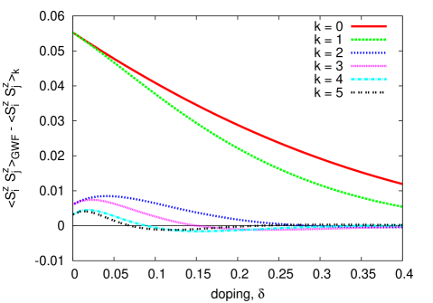
Figure 1: (Color online) Difference between the exact GWF results for the one-dimensional $t$-$J$ model and our DE-GWF results as a function of doping for orders $k=0\div 5$. The DE-GWF results change most when an even order is taken into account (e.g., inclusion of the fourth order terms gives bigger change than inclusion of the third). The largest discrepancy of the results is close to half filling, where the expansion parameter $x$ approaches its maximal absolute value of $|x|=4$.

The order $k$ to which we carry out our expansion, is not the only parameter affecting convergence. Another one is the number of $|\Psi_{0}\rangle$ lines (defined in Eq. (12)) included when calculating the diagrammatic sums. Its effect on results for the spin-spin correlation function is analyzed in Appendix D.

III Variational problem

In the previous section we have provided analytical results for the expectation values of all terms appearing in the Hamiltonian (1) with respect to the assumed wave function (6). These results enable us to calculate the ground state energy $W\equiv\langle\hat{H}\rangle_{G}$ for a fixed $|\Psi_{0}\rangle$. The remaining task is the minimization of this energy (or of the functional $\mathcal{F}\equiv W-2\mu_{G}n_{G}$, with $n_{G}\equiv\langle\hat{n}_{i\sigma}\rangle_{G}$) with respect to the wave function $|\Psi_{0}\rangle$. This wave function enters into the variational problem via $n\equiv\langle\hat{n}_{i\sigma}\rangle_{0}$ and the lines $P_{{\bf l},{\bf l}^{\prime}}$ and $S_{{\bf l},{\bf l}^{\prime}}$. In the following we consider only translationally invariant wave functions. Since we study superconducting states, the correlated and non-correlated numbers of particles ($n_{G}$ and $n$) may differ, and hence it is technically easier to minimize the functional $\mathcal{F}$ at a constant chemical potential $\mu_{G}$, and not the ground state energy at a constant number of particles $n_{G}$.

The remaining variational problem leads (cf. e.g. Refs. Yang et al., 2009; Wang et al., 2006; Bünemann et al., 2003) to the effective single-particle Schrödinger-like equation

$$\hat{H}_{0}^{\rm eff}|\Psi_{0}\rangle=E^{\rm eff}|\Psi_{0}\rangle,$$ (44)

with the self-consistently defined effective single-particle Hamiltonian

$$\hat{H}_{0}^{\rm eff} = \sum_{{\bf i},{\bf j},\sigma}t^{\rm eff}_{{\bf i},{\bf j}}\hat{c}_{{\bf i},\sigma}^{\dagger}\hat{c}_{{\bf j},\sigma}^{\phantom{\dagger}}+\sum_{{\bf i},{\bf j}}\big{(}\Delta^{\rm eff}_{{\bf i},{\bf j}}\hat{c}_{{\bf i},\uparrow}^{\dagger}\hat{c}_{{\bf j},\downarrow}^{\dagger}+{\rm H.c.}\big{)},$$ (45)

$$t^{\rm eff}_{{\bf i},{\bf j}} = \frac{\partial\mathcal{F}(|\Psi_{0}\rangle,x)}{\partial P_{{\bf i},{\bf j}}}\;,\qquad\Delta^{\rm eff}_{{\bf i},{\bf j}}=\frac{\partial\mathcal{F}(|\Psi_{0}\rangle,x)}{\partial S_{{\bf i},{\bf j}}}\;.$$ (46)

The effective dispersion relation, the effective gap, and eigenenergies of $\hat{H}_{0}^{\rm eff}$ are defined as

$$\varepsilon^{\rm eff}({\bf k}) = \frac{1}{L}\sum_{{\bf i},{\bf j}}\exp^{{\rm i}({\bf i}-{\bf j}){\bf k}}t^{\rm eff}_{{\bf i},{\bf j}}=\left[\sum_{{\bf j}}\exp^{{\rm i}({\bf i}-{\bf j}){\bf k}}t^{\rm eff}_{{\bf i},{\bf j}}\right]_{{\bf i}=(0,0)},$$ (47)

$$\Delta^{\rm eff}({\bf k}) = \frac{1}{L}\sum_{{\bf i},{\bf j}}\exp^{{\rm i}({\bf i}-{\bf j}){\bf k}}\Delta^{\rm eff}_{{\bf i},{\bf j}}=\left[\sum_{{\bf j}}\exp^{{\rm i}({\bf i}-{\bf j}){\bf k}}\Delta^{\rm eff}_{{\bf i},{\bf j}}\right]_{{\bf i}=(0,0)},$$ (48)

$$E^{\rm eff}({\bf k}) = \sqrt{\varepsilon^{\rm eff}({\bf k})^{2}+\Delta^{\rm eff}({\bf k})^{2}},$$ (49)

respectively, where the last expressions for $\varepsilon^{\rm eff}({\bf k})$ and $\Delta^{\rm eff}({\bf k})$ are valid for a homogeneous system. The final solution (of one iteration of our self-consistency loop) is obtained by solving Eqs. (44)-(46), with the additional minimization condition, $\partial_{x}\mathcal{F}(|\Psi_{0}\rangle,x)=0$. Having solved these equations, we can make the next iteration and calculate the new $|\Psi_{0}\rangle$ lines (from definition in Eq. (12)), according to the prescriptions

$$P_{{\bf l},{\bf m}} = \frac{1}{L}\sum_{\mathbf{k}}e^{i\mathbf{k}({\bf l}-{\bf m})}n_{\mathbf{k}}^{0},\qquad n_{\mathbf{k}}^{0}=\frac{1}{2}\left[1-\frac{\varepsilon^{\rm eff}({\bf k})}{E^{\rm eff}({\bf k})}\right],$$ (50)

$$S_{{\bf l},{\bf m}} = \frac{1}{L}\sum_{\mathbf{k}}e^{i\mathbf{k}({\bf l}-{\bf m})}\Delta_{\mathbf{k}}^{0},\qquad\Delta_{\mathbf{k}}^{0}=\frac{1}{2}\frac{\Delta^{\rm eff}({\bf k})}{E^{\rm eff}({\bf k})}.$$ (51)

The resulting self-consistency loop is shown in Fig. 2. The convergence is achieved when the new $|\Psi_{0}\rangle$ lines differ from the previous ones by less than the assumed precision value, typically $10^{-7}$.

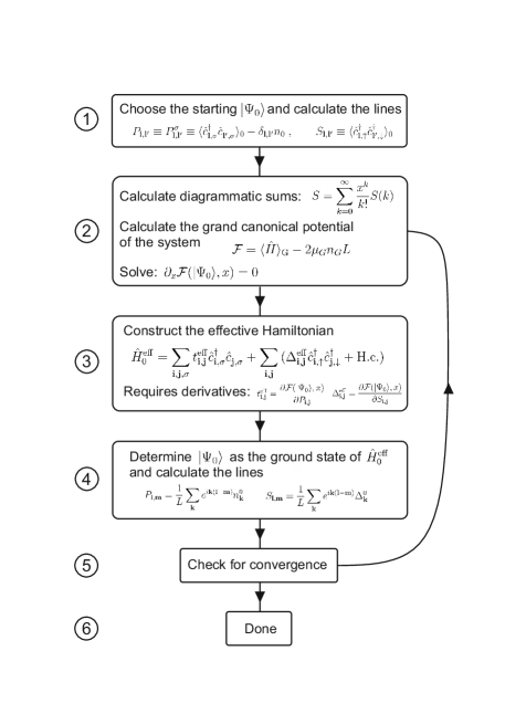
Figure 2: The full self-consistency loop of the DE-GWF method.

IV Results

The self-consistency loop in Fig. 2 is solved numerically with the use of GNU Scientific Library (GSL). The new lines are calculated from Eqs. (50)-(51) by numerical integration in $\mathbf{k}$ space (this corresponds to an infinite system size, $L\to\infty$). The typical accuracy of our solution procedure is equal to $10^{-7}$. We set $|t|=-t$ as our unit of energy and, unless stated otherwise, and present the results for $t^{\prime}=0.25$ and $J=0.3$. We consider the two cases with $c=0$ and $c=1$, but, as their results are very close, we show the $c=0$ data only in Figs. 4 and 5a. In several figures we provide also the results of the GCGA (and GA) methods, which were obtained by the simplified zeroth order DE-GWF method (equivalent to GCGA or GA, as discussed in Sec. II.5).

We carry out the expansion to the fifth order, which in most cases provides quite accurate results. The lower-order results are also exhibited in selected figures to visualize our method’s convergence. To calculate the diagrammatic sums we need to neglect long-range $|\Psi_{0}\rangle$-lines in real space. Namely, we take as nonzero only the lines $P_{{\bf i},{\bf j}}\equiv P_{0,({\bf i}-{\bf j})}\equiv P_{XY}$ (with $X=i_{1}-j_{1}$, $Y=i_{2}-j_{2}$), for which $X^{2}+Y^{2}\leq R^{2}=25$ (i.e., with 14 neighbors). The same condition applies for $S_{{\bf i},{\bf j}}$, $t^{\rm eff}_{{\bf i},{\bf j}}$, and $\Delta^{\rm eff}_{{\bf i},{\bf j}}$. We also define an additional convergence parameter. Namely, we take into account only those contributions to the diagrammatic sums, in which the total Manhattan distance (i.e., $|X|+|Y|$) of all lines is smaller than $R_{\rm tot}$ typically set to $R_{\rm tot}=26$.

In total, we have the three convergence parameters: (i) order $k$, (ii) $|\Psi_{0}\rangle$ cutoff radius $R$, (iii) total Manhattan distance of all lines $R_{\rm tot}$. The uncertainty of our results coming from parameters (ii) and (iii) is of the order of line thickness of the presented curves, whereas the $k$-th order results for most doping values are between the $k-1$ and $k-2$ order results (and the differences between them diminish with the increasing $k$). Therefore, we believe that the series is convergent. The accuracy of our results may be further improved by including higher order terms. However, in the sixth order there are already $10^{7}$ nonequivalent SC diagrams for the $T^{33}$ diagrammatic sum, what makes the analysis computationally demanding. Alternatively, as in the bold diagrammatic Monte Carlo technique Prokof’ev and Svistunov (2008); Van Houcke et al. (2012), a Cesàro-Riesz summation method could be used (cf. Ref. Prokof’ev and Svistunov, 2008, Sec. V.) to improve convergence of the diagrammatic sums. Work along these lines is planned.

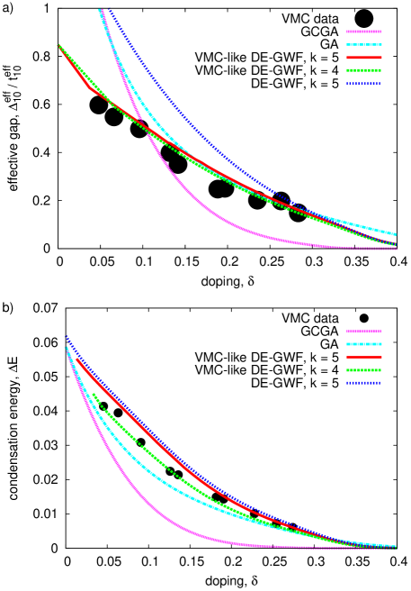
Figure 3: (Color online) Comparison of DE-GWF (lines) for $J=0.3$ and $t^{\prime}=0.3$ with variational Monte Carlo (VMC) results (the point size is equal to the error; from Ref. Edegger et al., 2006a). (a) Effective gap (in units of $t_{10}^{\rm eff}$) and (b) condensation energy as a function of doping. The VMC-like DE-GWF lines are obtained with effective single-particle Hamiltonian containing only (next)nearest-neighbor and on-site terms (see Appendix E for details). The fourth and fifth order results are shown for VMC-like DE-GWF to illustrate the convergence. The GA and GCGA results are obtained by the zeroth order DE-GWF.

To test our approach, in Figs. 3ab we have compared our results with those of Ref. Edegger et al., 2006a obtained by variational Monte Carlo (VMC) method for the Hamiltonian with $c=1$ and for the values of parameters $t^{\prime}=J=0.3$. In order to obtain comparable results we have to truncate our effective Hamiltonian, as in VMC, so that it contains parameters only up to next nearest-neighbors (see Appendix E for details). We call the resulting approach VMC-like DE-GWF. Its results agree very well with those of VMC. The sources of small quantitative discrepancies between the two results are due to approximations of both methods. First, in VMC calculations, a finite-size $11\times 11$ (or $13\times 13$) lattice is used, whereas we use an infinite lattice in the DE-GWF method. Note that in an analogous comparisonKaczmarczyk et al. (2013) with VMC calculations performed for the Hubbard model on an $8\times 8$ lattice, the discrepancies were much larger. Second, in our method we perform the expansion up to the 5th order (the remaining error coming from the $|\Psi_{0}\rangle$ cutoff in real space is of the order of line thickness).

Additionally, discrepancies might come from the fact that in our procedure the correlated ($n_{G}$) and uncorrelated ($n$) numbers of particles are slightly different, whereas it is not clear to us from Ref. Edegger et al., 2006a if there is a change in the particle number there due to the Gutzwiller projection.

The difference between the VMC-like DE-GWF and the full DE-GWF scheme shows that neglecting longer-range gap and hopping components can lead to a decrease of the principal gap component by up to $75\%$ (the largest discrepancy is near the half filling) and corresponding decrease of the condensation energy by $3\div 35\%$ (the largest discrepancy is for overdoped system). These discrepancies are larger than those observed in Ref. Watanabe et al., 2009, in which the longer-range hopping components were not included. Our results suggest that inclusion of the longer-range effective parameters is important as it can lead to changes of results even by a factor of 1.75, even though the condensation energy does not change much. We also provide GA and GCGA results to show their qualitative differences with respect to both VMC and DE-GWF. Surprisingly, GA is closer to the VMC and the DE-GWF results than its improved variant, GCGA. The largest discrepancy between GA and either VMC or DE-GWF data is for underdoped ($\delta<0.15$) and overdoped $\delta>0.3$ systems. We have also verified that for the zeroth order the VMC-like and the full DE-GWF methods yield the same results, as it should be, because the zeroth order diagrammatic sums only contain lines connecting (next)nearest neighbors.

The break in the VMC-like DE-GWF curve in Fig. 3a appearing at $\delta\approx 4\%$ is related to the phase separation effect present for the SC phase in the $t$-$J$ model in both (VMC-like)DE-GWF and VMC methods Ivanov (2004); Raczkowski et al. (2007); Chou and Lee (2012). Namely, the chemical potential ($\mu_{G}$) of the SC phase has a maximum as a function of doping for $\delta\approx 3\div 5\%$. For this reason, our numerical procedure (in which $\mu_{G}$ is increased at each step) fails to converge for $\delta\lesssim 5\%$. To obtain the following DE-GWF results we changed our method to work with a fixed $n_{G}$ (similarly, as in Refs. Kaczmarczyk and Spałek, 2011; Howczak et al., 2013; Zegrodnik et al., 2013; Abram et al., 2013, with an additional equation for $n_{G}$). This allowed us to obtain convergence in the vicinity of half filling.

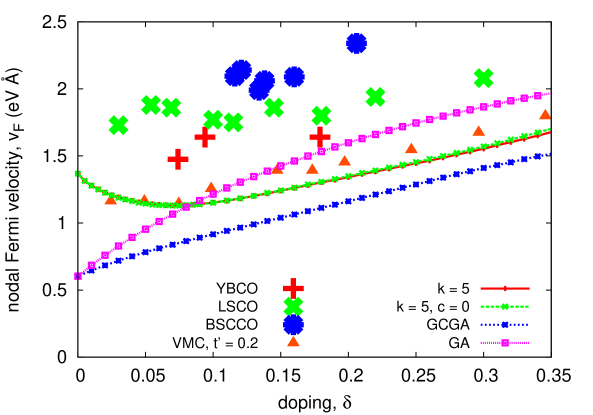
Figure 4: (color online) Universal Fermi velocity in the nodal ($k_{x}=k_{y}$) direction as a function of doping. The experimental values are taken from Ref. Edegger et al., 2006b and references therein and have typically an uncertainty of $20\%$. The VMC results are taken from Ref. Yunoki et al., 2005. The results obtained for the model with and without the density-density term (for $c=0$ and $c=1$, respectively) are very close.

One of the most important physical characteristics of the cuprates is the universal nodal Fermi velocity $v_{F}$ (i.e., $v_{F}$ is independent of $\delta$) Zhou et al. (2003). Recently, it has been shown however that the Fermi velocity for the underdoped samples exhibits a low-energy kink and a nontrivial doping dependence Vishik et al. (2010a). The velocity posesses the two components: one near the Fermi surface which is doping dependent and the velocity slightly below the Fermi surface which is doping independent. The source of the kink in the dispersion is probably the electron-phonon interaction Johnston et al. (2012) and is not included in our purely electronic model. In Fig. 4 we show the Fermi velocity defined as $v_{F}=\nabla_{\mathbf{k}}\epsilon^{\rm eff}(\mathbf{k})|_{\epsilon^{\rm eff}(\mathbf{k})=0}$. Its behavior agrees with the experimental results (we assume the lattice constant $a=4\,{\rm\AA}$ and $|t|=0.35\,{\rm eV}$). The RMFT method does not reproduce such behavior Jȩdrak and Spałek (2011); Edegger et al. (2006b). We also present for comparison the VMC results Yunoki et al. (2005); Paramekanti et al. (2001); Randeria et al. (2004); Paramekanti et al. (2004) obtained in Ref. Yunoki et al., 2005 for $t^{\prime}=0.2$. The weak doping dependence of the Fermi velocity speaks in favor of a transfer of the spectral density to the nodal direction from the antinodal direction with the decreasing doping (see also the discussion below).

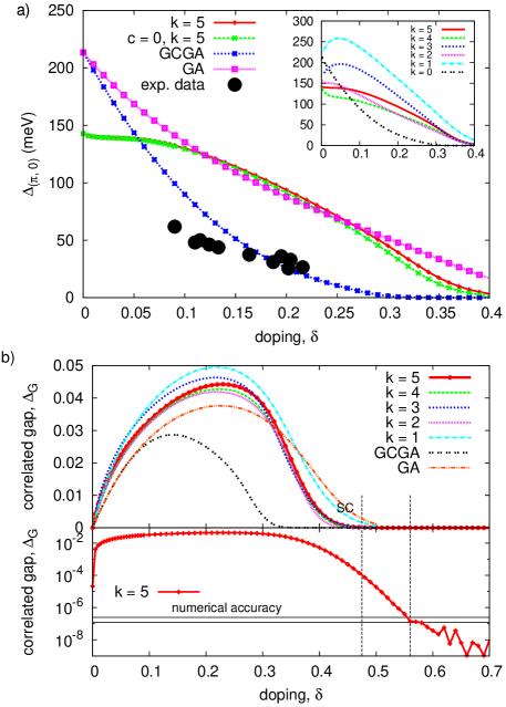
Figure 5: (Color online) (a) the effective gap at the antinodal point $\Delta^{\rm eff}_{\mathbf{k}=(\pi,0)}$ and its comparison with the experimental data of Ref. Campuzano et al., 1999; (b) the correlated gap $\Delta_{G}$. In (a) the gap values are plotted in physical units (assuming $t=0.35\,{\rm eV}$). The zeroth to fifth order results are exhibited to demonstrate the method convergence. In (b) we show also the gap on the logarithmic scale in the lower panel. We mark our numerical accuracy limit, which is around $10^{-7}$, by two horizontal lines. A residual very small gap persists to the dopings beyond the upper critical concentration (see also main text).

In Fig. 5 we plot the two gaps: the effective gap at the antinodal point $\Delta^{\rm eff}_{\mathbf{k}=(\pi,0)}$ and the correlated gap $\Delta_{G}$. The effective gap agrees with the experimental values only after rescaling by a factor of $0.4$ (not shown) similarly as for the GA Edegger et al. (2006b) and VMC Paramekanti et al. (2004) approaches. Recent experiments have shown however, that the competition between the superconducting gap and pseudogap Sacuto et al. (2013); Shekhter et al. (2013); Efetov et al. (2013) in BSCCO diminishes essentially the value of the superconducting gap in the nodal direction Kondo et al. (2009, 2010); Khasanov et al. (2008). In fact, this gap is shown to vanish for underdoped samples Kondo et al. (2009). Therefore, a quantitative agreement with the experimental points in Fig. 5a should not be the goal in describing high-temperature superconductors, as including the pseudogap may change the picture essentially. One should also keep in mind that $\Delta^{\rm eff}_{\mathbf{k}=(\pi,0)}$ depends on $J$. For lower $J$ values we obtain much better agreement with the experiment (but at the same time, the agreement of the nodal Fermi velocity is then worse). Similarly as in VMC calculations Yokoyama et al. (2013), we observe an exponential decay of the gap with the doping reaching the upper critical concentration $\delta_{c}\sim 1/2$. We term as SC the phase with $\Delta_{G}>10^{-4}$, which corresponds to gap values of the order of $0.4\,{\rm K}$, below which other effects can destabilize the superconductivity. In our model situation however, we still have a stable superconducting solution even if we increase doping above such defined $\delta_{c}$ by $8\%$. One must note that if the experimentally measured gap is usually determined for temperature $T\gtrsim 1{\rm K}$, then the tail of $\Delta_{G}(\delta)$ beyond $\delta_{c}$ will not be detected as then effectively $T>T_{c}$. In the inset of Fig. 5a and in the upper panel of Fig. 5b we show also the order-of-expansion dependence of the results. It can be seen that, for most of the doping values, the $k$-th order results are between the results obtained for order $k-1$ and $k-2$. Moreover, the difference between the orders diminishes with the increasing order.

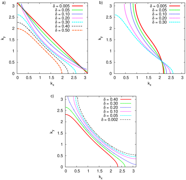
Figure 6: (Color online) (a) Fermi surfaces for selected values of doping in the normal phase (a), the spontaneously-distorted Pomeranchuk phase (b), and for the bare Hamiltonian with only kinetic energy without renormalization (c).

In the panel composing Fig. 6 we exhibit the doping dependence of the Fermi-surface topology, starting from the effective Hamiltonian (45). We also show results for the state with a spontaneously broken rotational symmetry, i.e., the appearance of the so-called Pomeranchuk phase Yamase and Kohno (2000a); *JPSJ.69.332; Halboth and Metzner (2000); Jȩdrak and Spałek (2010). This phase has also been investigated by VMC Edegger et al. (2006a); Zheng et al. . The drawback of using VMC in such calculations is that the finite-size effects become much more important than for the description of the SC phase (typically $12\times 12$ points Zheng et al. or $8\times 8$ points Edegger et al. (2006a) are included within the quarter of the Brillouin zone, cf. also the discussion in Ref. Edegger et al., 2006a). Our method does not suffer from those finite-size limitations and therefore, it seems more appropriate for analyzing the Fermi-surface properties. It can be seen from Fig. 6b that the correlated Fermi surface differs essentially from the non-interacting one near half filling. Namely, if we approach the half-filled case the Fermi surface becomes a line as in a bare Hamiltonian with the n.n. hopping only. This is caused by diminishing of certain effective hopping parameters in the vicinity of the half filling (as shown explicitly in Fig. 8b below). The doping dependence of the Fermi surface in the Pomeranchuk phase is similar to that obtained in the Hubbard model Bünemann et al. (2012). The role of the Pomeranchuk instability will not be studied in detail here.

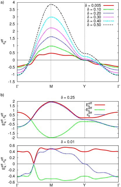
Figure 7: (Color online) (a) Dispersion relation of the effective Hamiltonian for the normal (paramagnetic) phase. The vertical lines mark specific points of the Brillouin zone: $\Gamma=(0,0)$, $M=(\pi,\pi)$, and $Y=(0,\pi)$. The horizontal line at $\varepsilon^{\rm eff}_{\mathbf{k}}=0$ marks the Fermi energy. (b) SC-phase quasiparticle energies for two doping values; the energies $\varepsilon_{\mathbf{k}}^{\rm eff}$ (of the normal phase at the same doping) are drawn for comparison.

The dispersion relation in the normal phase and the quasiparticle energies in the superconducting state are shown in Fig. 7. With the decreasing doping the bandwidth becomes smaller, and the dispersion deviates significantly from the simple form with the dominating n.n. hopping. The SC-phase quasiparticle energies (shown in Fig. 7b) resemble the metallic dispersion $\varepsilon^{\rm eff}_{\mathbf{k}}$ only for substantial doping values. With the decreasing doping deviations coming from the effective gap become larger. This effective gap has its maximum value (in the antinodal direction) close to the $Y$ point of the Brillouin zone. For small doping values this gap is comparable to the maximum value of $\varepsilon^{\rm eff}_{\mathbf{k}}$.

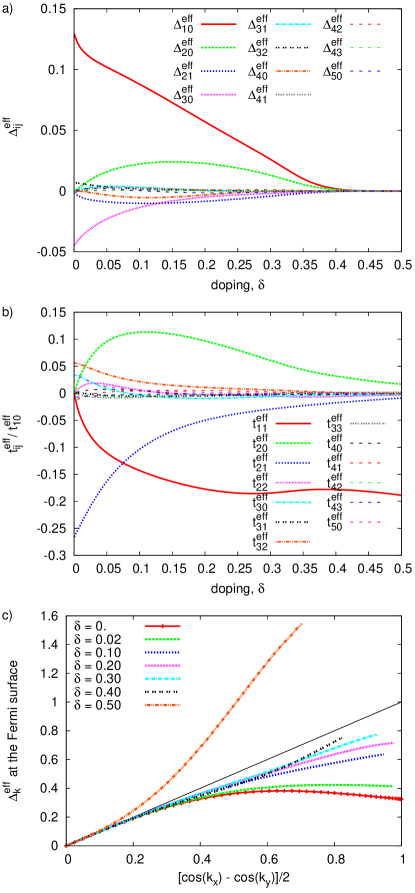
Figure 8: (Color online) (a) Effective gap parameters obtained variationally as a function of doping; (b) effective hopping parameters relative to the dominant $t_{10}^{\rm eff}$ contribution; (c) effective gap in momentum space at the Fermi energy for selected doping values. The black line corresponds to a pure $d_{x^{2}-y^{2}}$ dependence. The gaps are normalized for clarity.

In the panel composing Fig. 8 we detail the effective gap and the effective hopping amplitudes. Near half filling, only a few components of the gap are of substantial magnitude, namely $\Delta^{\rm eff}_{10}$, $\Delta^{\rm eff}_{21}$ (small, but nonzero), $\Delta^{\rm eff}_{30}$, and $\Delta^{\rm eff}_{32}$, as also found in Ref. Watanabe et al., 2009 (in which $[31]$ and $[40]$ are the most distant gap components). The same components of the effective hopping are nonzero at half filling, together with additional ones (e.g. $t^{\rm eff}_{50}$). From Fig. 8c it follows that the effective gap along the Fermi surface deviates from a pure $d_{x^{2}-y^{2}}$ form, especially close to half-filling, for which the gap in the antinodal direction is diminished by a factor of $3$ with respect to the pure $d_{x^{2}-y^{2}}$ form. Such deviations are also observed in high-temperature superconductors Mesot et al. (1999); Yoshida et al. (2012); Lee et al. (2007); Vishik et al. (2010b, 2012); Kondo et al. (2009, 2010); Khasanov et al. (2008), where the situation is complicated further by the appearance of pseudogap Shekhter et al. (2013); Efetov et al. (2013); Feng et al. (2012). Namely, for the underdoped samples the total gap measured in angle-resolved photoemission spectroscopy (ARPES) is increased in the antinodal direction with respect to the pure $d_{x^{2}-y^{2}}$ component Mesot et al. (1999); Yoshida et al. (2012); Lee et al. (2007); Vishik et al. (2010b, 2012), but the spectral weight corresponding to the superconducting gap is simultaneously decreased Kondo et al. (2009, 2010); Khasanov et al. (2008), which agrees with our findings in Fig. 8c. Therefore, such decrease of superconducting gap can be an intrinsic effect for strongly-correlated superconductors, not only caused by the competition with the pseudogap.

V Summary and Outlook

V.1 Methods comparison

When working with a variational Gutzwiller wave function, the main task is the calculation of the expectation value (Eq. (9)) of the Hamiltonian with respect to this trial wave function. So far, there have been two types of methods to approach this problem. In one of them (GA and the derivatives) the expectation values of the Hamiltonian terms are approximated by the corresponding expectation values with respect to the non-correlated wave function ($|\Psi_{0}\rangle$) multiplied by appropriate renormalization factors (e.g. $\langle\hat{c}^{\dagger}_{{\bf i},\sigma}\hat{c}_{{\bf j},\sigma}\rangle_{G}^{(GA)}=g_{t}\langle\hat{c}^{\dagger}_{{\bf i},\sigma}\hat{c}_{{\bf j},\sigma}\rangle_{0}$). This yields a very fast method, but constitutes an additional approximation, which prevents the description of superconductivity or Pomeranchuk phase in the Hubbard model. In contrast, VMC evaluates the expectation values in a controlled manner, but on a finite lattice, which leads to an increased numerical complexity of the approach. In DE-GWF the averages are also calculated as accurately as possible, but a different path towards computing them is undertaken. The resultant procedure leads to principal advantages over VMC: (i) the absence of the finite-size limitations, (ii) relatively low computational complexity, (iii) the ability to account for longer-range effective parameters in a natural manner (iv) the possibility of extending the approach to nonzero temperatures. On the other hand, VMC can be easily extended by introducing additional Jastrow factors to the trial wave function (this yields wavefunctions with, e.g., the doublon-holon correlation Yokoyama et al. (2004, 2013) or Baeriswyl wavefunctions Baeriswyl (2000); Hetényi (2010); Eichenberger and Baeriswyl (2007)). Investigation of the possibility of extending the DE-GWF method in this direction is planned.

V.2 Comparison with the Hubbard model results and the experiment

As the paper contains a new method of approach (DE-GWF) to high-temperature superconductivity analyzed within the $t$-$J$ model, a methodological note is in place here. Namely, we would like to relate the present results to those coming from our very recent analysis of the Hubbard model within DE-GWF Kaczmarczyk et al. (2013). First, the “dome-like” shape of $\Delta_{G}(\delta)$ is similar in both situations, particularly in the large-$U$ limit for the Hubbard model, though the upper critical concentration is lower in the latter case. Second, the doping independence of the Fermi velocity $v_{F}(\delta)$, representing a crucial test for any theory, is also closer to the experimental values in the Hubbard-model case. In both situations, DE-GWF provides much better values than those obtained within the dynamic mean-field theory (DMFT) Civelli et al. (2008). Third, the doping dependence of the gap in the antinodal direction (cf. Fig. 5a) can reproduce the experimental trend if we rescale the results by a factor of $\sim 1/2$ (see also below). Fourth, the deviations of the gap value along the Fermi surface from the $d_{x^{2}-y^{2}}$-wave symmetry are consistent with the experimental trend: diminishing of the superconducting gap in the antinodal region for underdoped samples.

V.3 Outlook

Combining the above features, together with a good agreement of the present results with the VMC analysis for small systems, DE-GWF provides a unique method of accounting for the basic superconducting properties in a quantitative manner. However, it fails to address one principal property, namely the appearance of the pseudogap. Very recently, we have generalized the analysis of the projected $t$-$J$ model Spałek by introducing in a systematic manner its supersymmetric (spin-fermion) representation. In this new representation, the Fermi sector provides essentially the $t$-$J$ model in the above fermionic representation, with an additional renormalization of both the hopping and the kinetic exchange integral amplitudes. This should diminish the scale of energies obtained theoretically in Fig. 5a (this idea requires still a detailed numerical analysis). What is even more interesting, the newest modelSpałek provides an explicit pairing and a separate scale of excitations in the Bose sector which may be interpreted as an appearance of a pseudogap. Summarizing, the new model preserves essential features of the $t$-$J$ model as discussed here, but introduces additionally the bosonic branch of collective phenomena. Such division is implicit in the recent calculations Feng et al. (2012). Work along this line is in progress and, as it requires a very complex numerical analysis, will be presented separately in the near future.

In conclusion, it is in our view rewarding that the Hubbard and the $t$-$J$ models provide converging results, at least on a semiquantitative level. To what extent this analysis can be enriched on the same level by a multiband model Hanke et al. (2010), remains to be seen.

Appendix A Exemplary types of diagrams

In Fig. 9 we present the diagram types for the kinetic energy ($T^{11}$, $T^{13}$, $T^{33}$), the potential energy ($I^{2}$, $I^{4}$), and the “correlated delta” ($S^{11}$, $S^{13}$, $S^{33}$) diagrammatic sums. We consider the first two orders (i.e., the diagrams with zero and one internal vertex). For the paramagnetic phase we would have only the diagrams without dashed lines (and obviously, no correlated delta diagrams). The number of diagrams grows exponentially with the increasing order $k$, and therefore we determine these diagrams by means of a numerical procedure.

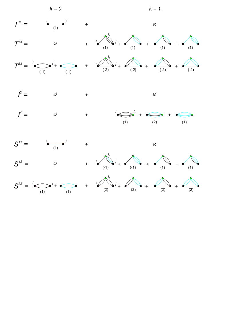
Figure 9: (color online). Diagrams in the zeroth and the first order. The superconducting (paramagnetic) contractions $S_{l,l^{\prime}}$ ($P_{l,l^{\prime}}$) are marked with dashed (solid) lines. The internal (external) vertices are marked with green (black) circles. The numbers in brackets below diagrams represent their multiplicity (a combinatorial factor).

The general form of the resulting diagrammatic sums is obtained as e.g.

$$T^{11} = P_{ij}+\mathcal{O}(x^{2}),$$ (53)

$$T^{13} = x\sum_{l_{1}}\Big{(}P_{il_{1}}P_{jl_{1}}^{3}+P_{il_{1}}P_{jl_{1}}S_{jl_{1}}^{2}+S_{il_{1}}P_{jl_{1}}^{2}S_{jl_{1}}+S_{il_{1}}S_{jl_{1}}^{3}\Big{)}+\mathcal{O}(x^{2}),$$ (54)

$$S^{13} = x\sum_{l_{1}}\Big{(}-P_{il_{1}}P_{jl_{1}}^{2}S_{jl_{1}}-P_{il_{1}}S_{jl_{1}}^{3}+S_{il_{1}}P_{jl_{1}}^{3}+S_{il_{1}}S_{jl_{1}}^{2}P_{jl_{1}}\Big{)}+\mathcal{O}(x^{2}).$$ (55)

In order to perform the summations of diagrams over a lattice, we need to assume as nonzero the $|\Psi_{0}\rangle$ lines up to some finite distance. In the main text we have taken as nonzero the lines ($S_{{\bf i},{\bf j}}\equiv S_{X,Y}$ with $X=(i_{1}-j_{1}),Y=(i_{2}-j_{2})$, $P_{X,Y}$ - analogously) fulfilling $X^{2}+Y^{2}\leq R^{2}=25$. If the cutoff distance is defined by $X^{2}+Y^{2}\leq 2$, then they are as follows

$$T^{11}(0) = P_{10},$$ (56)

$$T^{33}(0) = -P_{10}^{3}-P_{10}S_{10}^{2},$$ (57)

$$T^{13}(1) = 2P_{10}^{3}P_{11}+2P_{10}P_{11}^{3}+2P_{10}P_{11}S_{10}^{2}.$$ (58)

Increasing the cutoff distance $R$ leads to significant complication of the obtained expressions - e.g. for $X^{2}+Y^{2}\leq 4$ (allowing for nonzero $P_{20}$ and $S_{20}$ lines), we have

$$T^{13}(1) = 2P_{10}^{3}P_{11}+2P_{10}P_{11}^{3}+2P_{10}P_{11}S_{10}^{2}+P_{10}^{3}P_{20}+S_{10}S_{20}^{3}+P_{10}^{2}S_{10}S_{20}$$ (59)

$$+P_{20}^{2}S_{10}S_{20}+2P_{10}P_{11}S_{10}^{2}+S_{10}^{3}S_{20}+P_{10}P_{20}S_{20}^{2}.$$

In our numerical procedure, when calculating the diagrammatic sums, we start from the general form (as in Eqs. (53) - (55)) and sum over the internal vertices positions (here over ${\bf l}_{1}$) making sure that the condition $X^{2}+Y^{2}\leq 25$ is fulfilled for all contributing lines $P_{X,Y}$, $S_{X,Y}$.

Appendix B Exchange term evaluation

The expressions for the components of the exchange term are as follows (with $m_{i}\equiv n_{i\uparrow}-n_{i\downarrow}$)

$$\frac{1}{4}\langle\hat{n}_{\bf i}\hat{n}_{\bf j}\rangle_{G} = +\frac{n_{\bf i}n_{\bf j}}{4}+\frac{(n_{\bf i}-1)(n_{\bf j}-1)I_{{\bf i}{{\bf j}\downarrow}}^{42}}{2(n_{{{\bf i}\downarrow}}-1)(n_{{{\bf i}\uparrow}}-1)(n_{{{\bf j}\downarrow}}-1)}+\frac{(n_{\bf i}-1)(n_{\bf j}-1)I_{{\bf i}{{\bf j}\uparrow}}^{42}}{2(n_{{{\bf i}\downarrow}}-1)(n_{{{\bf i}\uparrow}}-1)(n_{{{\bf j}\uparrow}}-1)}+$$ (60)

$$\frac{(n_{\bf i}-1)(n_{\bf j}-1)I_{{{\bf i}\downarrow}{\bf j}}^{24}}{2(n_{{{\bf i}\downarrow}}-1)(n_{{{\bf j}\downarrow}}-1)(n_{{{\bf j}\uparrow}}-1)}+\frac{(n_{\bf i}-1)(n_{\bf j}-1)I_{{{\bf i}\downarrow}{{\bf j}\downarrow}}^{22}}{4(n_{{{\bf i}\downarrow}}-1)(n_{{{\bf j}\downarrow}}-1)}+\frac{(n_{\bf i}-1)(n_{\bf j}-1)I_{{{\bf i}\downarrow}{{\bf j}\uparrow}}^{22}}{4(n_{{{\bf i}\downarrow}}-1)(n_{{{\bf j}\uparrow}}-1)}+$$

$$\frac{(n_{\bf i}-1)(n_{\bf j}-1)I_{{{\bf i}\uparrow}{\bf j}}^{24}}{2(n_{{{\bf i}\uparrow}}-1)(n_{{{\bf j}\downarrow}}-1)(n_{{{\bf j}\uparrow}}-1)}+\frac{(n_{\bf i}-1)(n_{\bf j}-1)I_{{{\bf i}\uparrow}{{\bf j}\downarrow}}^{22}}{4(n_{{{\bf i}\uparrow}}-1)(n_{{{\bf j}\downarrow}}-1)}+\frac{(n_{\bf i}-1)(n_{\bf j}-1)I_{{{\bf i}\uparrow}{{\bf j}\uparrow}}^{22}}{4(n_{{{\bf i}\uparrow}}-1)(n_{{{\bf j}\uparrow}}-1)}+$$

$$\frac{I_{{{\bf j}\uparrow}}^{2}n_{\bf i}(n_{\bf j}-1)}{4(n_{{{\bf j}\uparrow}}-1)}+\frac{I_{{{\bf j}\downarrow}}^{2}n_{\bf i}(n_{\bf j}-1)}{4(n_{{{\bf j}\downarrow}}-1)}+\frac{I_{{{\bf i}\uparrow}}^{2}(n_{\bf i}-1)n_{\bf j}}{4(n_{{{\bf i}\uparrow}}-1)}+\frac{I_{\bf i}^{4}(n_{\bf i}-1)n_{\bf j}}{2(n_{{{\bf i}\downarrow}}-1)(n_{{{\bf i}\uparrow}}-1)}+$$

$$\frac{I_{{{\bf i}{\bf j}}}^{44}(n_{\bf i}-1)(n_{\bf j}-1)}{(n_{{{\bf i}\downarrow}}-1)(n_{{{\bf i}\uparrow}}-1)(n_{{{\bf j}\downarrow}}-1)(n_{{{\bf j}\uparrow}}-1)}+\frac{I_{{{\bf i}\downarrow}}^{2}(n_{\bf i}-1)n_{\bf j}}{4(n_{{{\bf i}\downarrow}}-1)}+\frac{I_{\bf j}^{4}n_{\bf i}(n_{\bf j}-1)}{2(n_{{{\bf j}\downarrow}}-1)(n_{{{\bf j}\uparrow}}-1)}.$$

$$\langle\hat{S}_{\bf i}^{z}\hat{S}_{\bf j}^{z}\rangle_{G} = \frac{m_{\bf i}m_{\bf j}}{4}+\frac{m_{\bf i}(m_{\bf j}+1)I_{{\bf i}{{\bf j}\downarrow}}^{42}}{2(n_{{{\bf i}\downarrow}}-1)(n_{{{\bf i}\uparrow}}-1)(n_{{{\bf j}\downarrow}}-1)}-\frac{m_{\bf i}(1-m_{\bf j})I_{{\bf i}{{\bf j}\uparrow}}^{42}}{2(n_{{{\bf i}\downarrow}}-1)(n_{{{\bf i}\uparrow}}-1)(n_{{{\bf j}\uparrow}}-1)}-$$ (61)

$$\frac{(-m_{\bf i}-1)m_{\bf j}I_{{{\bf i}\downarrow}{\bf j}}^{24}}{2(n_{{{\bf i}\downarrow}}-1)(n_{{{\bf j}\downarrow}}-1)(n_{{{\bf j}\uparrow}}-1)}+\frac{(-m_{\bf i}-1)(-m_{\bf j}-1)I_{{{\bf i}\downarrow}{{\bf j}\downarrow}}^{22}}{4(n_{{{\bf i}\downarrow}}-1)(n_{{{\bf j}\downarrow}}-1)}+\frac{(-m_{\bf i}-1)(1-m_{\bf j})I_{{{\bf i}\downarrow}{{\bf j}\uparrow}}^{22}}{4(n_{{{\bf i}\downarrow}}-1)(n_{{{\bf j}\uparrow}}-1)}-$$

$$\frac{(-m_{\bf i}+1)m_{\bf j}I_{{{\bf i}\uparrow}{\bf j}}^{24}}{2(n_{{{\bf i}\uparrow}}-1)(n_{{{\bf j}\downarrow}}-1)(n_{{{\bf j}\uparrow}}-1)}+\frac{(-m_{\bf i}+1)(-m_{\bf j}-1)I_{{{\bf i}\uparrow}{{\bf j}\downarrow}}^{22}}{4(n_{{{\bf i}\uparrow}}-1)(n_{{{\bf j}\downarrow}}-1)}+\frac{(-m_{\bf i}+1)(1-m_{\bf j})I_{{{\bf i}\uparrow}{{\bf j}\uparrow}}^{22}}{4(n_{{{\bf i}\uparrow}}-1)(n_{{{\bf j}\uparrow}}-1)}+$$

$$\frac{I_{{{\bf j}\uparrow}}^{2}m_{\bf i}(1-m_{\bf j})}{4(1-n_{{{\bf j}\uparrow}})}+\frac{I_{{{\bf j}\downarrow}}^{2}m_{\bf i}(-m_{\bf j}-1)}{4(1-n_{{{\bf j}\downarrow}})}-\frac{I_{{{\bf i}\uparrow}}^{2}(-m_{\bf i}+1)m_{\bf j}}{4(n_{{{\bf i}\uparrow}}-1)}+$$

$$\frac{I_{{\bf i}{\bf j}}^{44}m_{\bf i}m_{\bf j}}{(n_{{{\bf i}\downarrow}}-1)(n_{{{\bf i}\uparrow}}-1)(n_{{{\bf j}\downarrow}}-1)(n_{{{\bf j}\uparrow}}-1)}-\frac{I_{{{\bf i}\downarrow}}^{2}(m_{\bf i}+1)m_{\bf j}}{4(1-n_{{{\bf i}\downarrow}})}+\frac{I^{\bf j}_{4}m_{\bf i}m_{\bf j}}{2(1-n_{{{\bf j}\downarrow}})(1-n_{{{\bf j}\uparrow}})}+$$

$$\frac{I^{\bf i}_{4}m_{\bf i}m_{\bf j}}{2(1-n_{{{\bf i}\downarrow}})(1-n_{{{\bf i}\uparrow}})}.$$

Appendix C Gutzwiller factors change

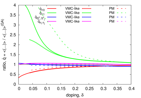
Figure 10: (Color online) The ratio of the averages $\langle(...)\rangle_{G}$ obtained in (VMC-like)DE-GWF with respect to that obtained in GA.

In Fig. 10 we plot the ratio of the averages $\langle(...)\rangle_{G}$ obtained accurately within (VMC-like)DE-GWF (Eqs. (29)-(32)) and those obtained by within Gutzwiller approximation (Eqs. (38)-(40)). Explicitly, we plot the following quantities

$$\overline{q}_{{\bf i}{\bf j}} \equiv \frac{\langle\hat{c}^{\dagger}_{{\bf i},\sigma}\hat{c}_{{\bf j},\sigma}\rangle_{G}}{\langle\hat{c}^{\dagger}_{{\bf i},\sigma}\hat{c}_{{\bf j},\sigma}\rangle_{G}^{(GA)}}=\frac{q^{2}T^{11}_{{\bf i}{\bf j}}+2q\alpha T^{13}_{{\bf i}{\bf j}}+\alpha^{2}T^{33}_{{\bf i}{\bf j}}}{q^{2}P_{{\bf i}{\bf j}}},$$ (62)

$$\overline{q}_{S_{i}^{z}S_{j}^{z}} \equiv \frac{\langle\hat{S}_{\bf i}^{+}\hat{S}_{\bf j}^{-}+\hat{S}_{\bf i}^{-}\hat{S}_{\bf j}^{+}\rangle_{G}}{\langle\hat{S}_{\bf i}^{+}\hat{S}_{\bf j}^{-}+\hat{S}_{\bf i}^{-}\hat{S}_{\bf j}^{+}\rangle_{G}^{(GA)}}=\frac{2S^{22}}{\langle\hat{S}_{\bf i}^{+}\hat{S}_{\bf j}^{-}+\hat{S}_{\bf i}^{-}\hat{S}_{\bf j}^{+}\rangle_{0}}=\frac{S^{22}}{S^{22}(0)},$$ (63)

$$\overline{q}_{n_{i}n_{j}} \equiv \frac{\langle\hat{n}_{\bf i}\hat{n}_{\bf j}\rangle_{G}}{\langle\hat{n}_{\bf i}\hat{n}_{\bf j}\rangle_{G}^{(GA)}}=\frac{n^{2}+I^{22\uparrow\uparrow}\gamma+I^{22\uparrow\downarrow}\gamma+(...)}{n^{2}+I^{22\uparrow\uparrow}(0)\gamma+I^{22\uparrow\downarrow}(0)\gamma}.$$ (64)

where $\gamma\equiv\frac{\left(1-2n\right){}^{2}}{2\left(n-1\right){}^{2}}$, by e.g. $S^{22}(0)$ we understand the zeroth-order diagrammatic sum, and by (…) we denote other diagrammatic sum terms, (see Eq. (32)). According to the above expressions, a situation in which GA approximates the average accurately corresponds to $\overline{q}=1$. If an average is overestimated (underestimated) by GA, this yields $\overline{q}<1$ ($\overline{q}>1$). It can be seen from Fig. 10 that for the exchange term averages $\overline{q}\approx 1$, and therefore GA works quite well for them. However, for the kinetic energy term averages GA largely overestimates the n.n. average (as also reported in Ref. Fukushima, 2008) and underestimates the next n.n. average, especially for an underdoped system. This is the reason behind the large discrepancy of the GA and VMC results in this regime. The ratios $\overline{q}$ are quite similar in VMC-like and full DE-GWF methods. They are also similar in the PM phase (however, for the next n.n. hopping the ratio $\overline{q}_{11}$is substantially larger).

Appendix D Convergence analysis: number of lines

To analyze the effect of number of $|\Psi_{0}\rangle$ lines included in the calculations we present in Fig. 11 the difference (integrated over doping values) between the correlation function $\langle\hat{S}_{\bf i}^{z}\hat{S}_{\bf j}^{z}\rangle$ for a given number of lines $n$ and for 25 lines as a function of $n$.

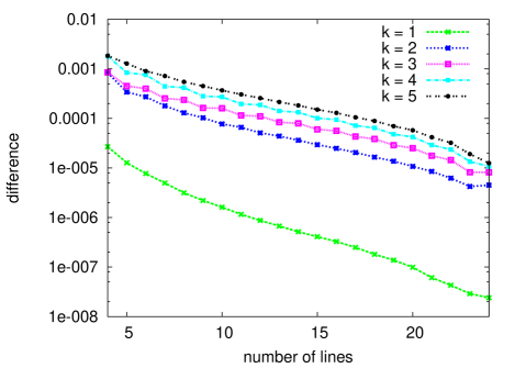
Figure 11: (Color online) Convergence of the results for $\langle\hat{S}_{\bf i}^{z}\hat{S}_{\bf j}^{z}\rangle$ as a function of number of $|\Psi_{0}\rangle$ lines.

Nearly linear behavior of the differences in Fig. 11 suggests that the convergence is exponential (a logarithmic scale is used in Fig. 11). Note also that the higher-order results converge more slowly than the lower-order results, what indicates that to obtain the same accuracy (with respect to the complete $|\Psi_{0}\rangle$ results with all lines included) in a higher order we need to take into account more lines than in a lower order. Therefore, not only the inclusion of higher-order terms is important to improve accuracy, but also the inclusion of longer range lines.

Appendix E Details of the VMC-like DE-GWF calculations

We set all parameters of the effective Hamiltonian to zero, except for n.n. pairing $\Delta^{\rm eff}_{10}$ and hoppings $t^{\rm eff}_{10}$, $t^{\rm eff}_{11}$, as well as $t^{\rm eff}_{00}$ playing the role of effective chemical potential. The n.n. hopping is kept fixed, whereas the other parameters are optimized variationally. In the resulting scheme the effective Hamiltonian contains the same variational parameters as that used in VMC Edegger et al. (2006a).

We have taken as nonzero the $|\Psi_{0}\rangle$ lines ($S_{{\bf i},{\bf j}}\equiv S_{0,({\bf i}-{\bf j})}\equiv S_{XY}$ with $X=(i_{1}-j_{1}),Y=(i_{2}-j_{2})$, $P_{XY}$ - analogously) fulfilling $X^{2}+Y^{2}\leq 25$. In the situation when the number of $|\Psi_{0}\rangle$ lines does not match the number of effective parameters ($t_{{\bf i},{\bf j}}^{\rm eff}$ and $\Delta_{{\bf i},{\bf j}}^{\rm eff}$), the self-consistency loop would not find the true minimum of the energy and a more standard minimization of the energy with respect to $\Delta^{\rm eff}_{10}$, $t^{\rm eff}_{00}$, and $t^{\rm eff}_{11}$ is necessary. Namely, we numerically search for a minimum of the system grand canonical potential $\mathcal{F}$ by calculating its value for fixed $\Delta^{\rm eff}_{10}$, $t^{\rm eff}_{00}$, and $t^{\rm eff}_{11}$. The flowchart of such calculations is presented in Fig. 12. Explicitly, having fixed effective parameters (step 1 in Fig. 12) we may construct the effective Hamiltonian (step 2), calculate the $|\Psi_{0}\rangle$ lines (step 3), and having them we can obtain the diagrammatic sums and the potential $\mathcal{F}$ (step 4). Finally, we choose the solution with $\Delta^{\rm eff}_{10}$, $t^{\rm eff}_{00}$, and $t^{\rm eff}_{11}$ corresponding to the lowest potential $\mathcal{F}$.

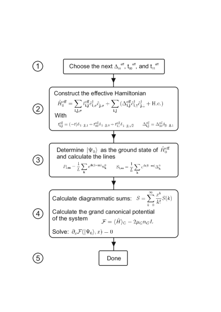
Figure 12: Flowchart of the VMC-like DE-GWF calculations.

References

- Lee et al. (2006) P. A. Lee, N. Nagaosa, and X.-G. Wen, Rev. Mod. Phys. 78, 17 (2006).
- Ogata and Fukuyama (2008) M. Ogata and H. Fukuyama, Rep. Prog. Phys. 71, 036501 (2008).
- Scalapino (2012) D. J. Scalapino, Rev. Mod. Phys. 84, 1383 (2012).
- Edegger et al. (2007) B. Edegger, V. N. Muthukumar, and C. Gros, Adv. Phys. 56, 927 (2007).
- Anderson (2007) P. Anderson, Science 317, 1705 (2007).
- Spałek and Goc-Jagło (2012) J. Spałek and D. Goc-Jagło, Phys. Scr. 86, 048301 (2012).
- Maier et al. (2006a) T. A. Maier, M. S. Jarrell, and D. J. Scalapino, Phys. Rev. Lett. 96, 047005 (2006a).
- Maier et al. (2006b) T. A. Maier, M. S. Jarrell, and D. J. Scalapino, Phys. Rev. B 74, 094513 (2006b).
- Monthoux et al. (1991) P. Monthoux, A. V. Balatsky, and D. Pines, Phys. Rev. Lett. 67, 3448 (1991).
- Kyung et al. (2009) B. Kyung, D. Sénéchal, and A.-M. S. Tremblay, Phys. Rev. B 80, 205109 (2009).
- Hanke et al. (2010) W. Hanke, M. Kiesel, M. Aichhorn, S. Brehm, and E. Arrigoni, Eur. Phys. J. Special Topics 188, 15 (2010).
- Anderson (1988) P. W. Anderson, Frontiers and Borderlines in Many-Particle Physics, edited by R. A. Broglia and J. R. Schrieffer (North-Holland, Amsterdam, 1988) pp. 1–40.
- Zhang and Rice (1988) F. C. Zhang and T. M. Rice, Phys. Rev. B 37, 3759 (1988).
- Zhang and Rice (1990) F. C. Zhang and T. M. Rice, Phys. Rev. B 41, 7243 (1990).
- Spałek (1988a) J. Spałek, Phys. Rev. B 37, 533 (1988a).
- Spałek (1988b) J. Spałek, Phys. Rev. B 38, 208 (1988b).
- Gutzwiller (1963) M. C. Gutzwiller, Phys. Rev. Lett. 10, 159 (1963).
- Gutzwiller (1965) M. C. Gutzwiller, Phys. Rev. 137, A1726 (1965).
- Zhang et al. (1988) F. C. Zhang, C. Gros, T. M. Rice, and H. Shiba, Supercond. Sci. Technol. 1, 36 (1988).
- Ogata and Himeda (2003) M. Ogata and A. Himeda, J. Phys. Soc. Jpn. 72, 374 (2003).
- Wang et al. (2006) Q.-H. Wang, Z. D. Wang, Y. Chen, and F. C. Zhang, Phys. Rev. B 73, 092507 (2006).
- Fukushima (2008) N. Fukushima, Phys. Rev. B 78, 115105 (2008).
- Fukushima (2011) N. Fukushima, J. Phys. A: Math. Theor. 44, 075002 (2011).
- Jȩdrak and Spałek (2011) J. Jȩdrak and J. Spałek, Phys. Rev. B 83, 104512 (2011).
- Jȩdrak and Spałek (2010) J. Jȩdrak and J. Spałek, Phys. Rev. B 81, 073108 (2010).
- Kaczmarczyk and Spałek (2011) J. Kaczmarczyk and J. Spałek, Phys. Rev. B 84, 125140 (2011).
- Howczak et al. (2013) O. Howczak, J. Kaczmarczyk, and J. Spałek, Phys. Status Solidi (b) 250, 609 (2013).
- Zegrodnik et al. (2013) M. Zegrodnik, J. Spałek, and J. Bünemann, New J. Phys. 15, 073050 (2013).
- Abram et al. (2013) M. Abram, J. Kaczmarczyk, J. Jȩdrak, and J. Spałek, Phys. Rev. B 88, 094502 (2013).
- Bünemann et al. (2012) J. Bünemann, T. Schickling, and F. Gebhard, Europhys. Lett. 98, 27006 (2012).
- Kaczmarczyk et al. (2013) J. Kaczmarczyk, J. Spałek, T. Schickling, and J. Bünemann, Phys. Rev. B 88, 115127 (2013).
- Metzner and Vollhardt (1988) W. Metzner and D. Vollhardt, Phys. Rev. B 37, 7382 (1988).
- Kurzyk et al. (2007) J. Kurzyk, J. Spałek, and J. Wójcik, Acta Phys. Polon. A 111, 603 (2007).
- Note (1) For original derivation of the - model from the Hubbard model see: K. A. Chao, J. Spałek, and A. M. Oleś, J. Phys. C 10, L271 (1977). For didactical exposition see: J. Spałek, Acta Phys. Polon. A 121, 764 (2012).
- Gebhard (1990) F. Gebhard, Phys. Rev. B 41, 9452 (1990).
- Fetter and Walecka (2003) A. L. Fetter and J. D. Walecka, Quantum Theory of Many-Particle Systems (Dover Publications, New York, 2003).
- Note (2) The numerical difference between the results of the zeroth order DE-GWF and GCGA is smaller than the line thickness of the presented curves, so neglecting of the diagrammatic sum is not essential.
- Gebhard and Vollhardt (1988) F. Gebhard and D. Vollhardt, Phys. Rev. B 38, 6911 (1988).
- Yang et al. (2009) K.-Y. Yang, W. Q. Chen, T. M. Rice, M. Sigrist, and F.-C. Zhang, New J. Phys. 11, 055053 (2009).
- Bünemann et al. (2003) J. Bünemann, F. Gebhard, and R. Thul, Phys. Rev. B 67, 075103 (2003).
- Prokof’ev and Svistunov (2008) N. V. Prokof’ev and B. V. Svistunov, Phys. Rev. B 77, 125101 (2008).
- Van Houcke et al. (2012) K. Van Houcke, F. Werner, E. Kozik, N. Prokof’ev, B. Svistunov, M. J. H. Ku, A. T. Sommer, L. W. Cheuk, A. Schirotzek, and M. W. Zwierlein, Nature Phys. 8, 366 (2012).
- Edegger et al. (2006a) B. Edegger, V. N. Muthukumar, and C. Gros, Phys. Rev. B 74, 165109 (2006a).
- Watanabe et al. (2009) T. Watanabe, H. Yokoyama, K. Shigeta, and M. Ogata, New J. Phys. 11, 075011 (2009).
- Ivanov (2004) D. A. Ivanov, Phys. Rev. B 70, 104503 (2004).
- Raczkowski et al. (2007) M. Raczkowski, M. Capello, D. Poilblanc, R. Frésard, and A. M. Oleś, Phys. Rev. B 76, 140505 (2007).
- Chou and Lee (2012) C.-P. Chou and T.-K. Lee, Phys. Rev. B 85, 104511 (2012).
- Edegger et al. (2006b) B. Edegger, V. N. Muthukumar, C. Gros, and P. W. Anderson, Phys. Rev. Lett. 96, 207002 (2006b).
- Yunoki et al. (2005) S. Yunoki, E. Dagotto, and S. Sorella, Phys. Rev. Lett. 94, 037001 (2005).
- Zhou et al. (2003) X. J. Zhou, T. Yoshida, A. Lanzara, P. V. Bogdanov, S. A. Kellar, K. M. Shen, W. L. Yang, F. Ronning, T. Sasagawa, T. Kakeshita, T. Noda, H. Eisaki, S. Uchida, C. T. Lin, F. Zhou, J. W. Xiong, W. X. Ti, Z. X. Zhao, A. Fujimori, Z. Hussain, and Z.-X. Shen, Nature 423, 398 (2003).
- Vishik et al. (2010a) I. M. Vishik, W. S. Lee, F. Schmitt, B. Moritz, T. Sasagawa, S. Uchida, K. Fujita, S. Ishida, C. Zhang, T. P. Devereaux, and Z. X. Shen, Phys. Rev. Lett. 104, 207002 (2010a).
- Johnston et al. (2012) S. Johnston, I. M. Vishik, W. S. Lee, F. Schmitt, S. Uchida, K. Fujita, S. Ishida, N. Nagaosa, Z. X. Shen, and T. P. Devereaux, Phys. Rev. Lett. 108, 166404 (2012).
- Paramekanti et al. (2001) A. Paramekanti, M. Randeria, and N. Trivedi, Phys. Rev. Lett. 87, 217002 (2001).
- Randeria et al. (2004) M. Randeria, A. Paramekanti, and N. Trivedi, Phys. Rev. B 69, 144509 (2004).
- Paramekanti et al. (2004) A. Paramekanti, M. Randeria, and N. Trivedi, Phys. Rev. B 70, 054504 (2004).
- Campuzano et al. (1999) J. C. Campuzano, H. Ding, M. R. Norman, H. M. Fretwell, M. Randeria, A. Kaminski, J. Mesot, T. Takeuchi, T. Sato, T. Yokoya, T. Takahashi, T. Mochiku, K. Kadowaki, P. Guptasarma, D. G. Hinks, Z. Konstantinovic, Z. Z. Li, and H. Raffy, Phys. Rev. Lett. 83, 3709 (1999).
- Sacuto et al. (2013) A. Sacuto, S. Benhabib, Y. Gallais, S. Blanc, M. Cazayous, M.-A. M asson, J. S. Wen, Z. J. Xu, and G. D. Gu, J. Phys.: Conf. Ser. 449, 012011 (2013).
- Shekhter et al. (2013) A. Shekhter, B. J. Ramshaw, R. Liang, W. N. Hardy, D. A. Bonn, F. F. Balakirev, R. D. McDonald, J. B. Betts, S. C. Riggs, and A. Migliori, Nature 498, 75 (2013).
- Efetov et al. (2013) K. B. Efetov, H. Meier, and C. Pepin, Nature Phys. 9, 442 (2013).
- Kondo et al. (2009) T. Kondo, R. Khasanov, T. Takeuchi, J. Schmalian, and A. Kaminski, Nature 457, 296 (2009).
- Kondo et al. (2010) T. Kondo, Y. Hamaya, A. D. Palczewski, T. Takeuchi, J. S. Wen, G. Gu, J. Schmalian, and A. Kaminski, Nature Phys. 7, 21 (2010).
- Khasanov et al. (2008) R. Khasanov, T. Kondo, S. Strässle, D. O. G. Heron, A. Kaminski, H. Keller, S. L. Lee, and T. Takeuchi, Phys. Rev. Lett. 101, 227002 (2008).
- Yokoyama et al. (2013) H. Yokoyama, M. Ogata, Y. Tanaka, K. Kobayashi, and H. Tsuchiura, J. Phys. Soc. Jpn. 82, 014707 (2013).
- Yamase and Kohno (2000a) H. Yamase and H. Kohno, Journal of the Physical Society of Japan 69, 2151 (2000a).
- Yamase and Kohno (2000b) H. Yamase and H. Kohno, Journal of the Physical Society of Japan 69, 332 (2000b).
- Halboth and Metzner (2000) C. J. Halboth and W. Metzner, Phys. Rev. Lett. 85, 5162 (2000).
- (67) X.-J. Zheng, Z.-B. Huang, and L.-J. Zou, arXiv:1301.1012.
- Mesot et al. (1999) J. Mesot, M. R. Norman, H. Ding, M. Randeria, J. C. Campuzano, A. Paramekanti, H. M. Fretwell, A. Kaminski, T. Takeuchi, T. Yokoya, T. Sato, T. Takahashi, T. Mochiku, and K. Kadowaki, Phys. Rev. Lett. 83, 840 (1999).
- Yoshida et al. (2012) T. Yoshida, M. Hashimoto, I. M. Vishik, Z.-X. Shen, and A. Fujimori, J. Phys. Soc. Jpn. 81, 011006 (2012).
- Lee et al. (2007) W. Lee, I. Vishik, K. Tanaka, D. Lu, T. Sasagawa, N. Nagaosa, T. Devereaux, Z. Hussain, and Z.-X. Shen, Nature 450, 81 (2007).
- Vishik et al. (2010b) I. M. Vishik, W. S. Lee, R.-H. He, M. Hashimoto, Z. Hussain, T. P. Devereaux, and Z.-X. Shen, New J. Phys. 12, 105008 (2010b).
- Vishik et al. (2012) I. M. Vishik, M. Hashimoto, R.-H. He, W.-S. Lee, F. Schmitt, D. Lu, R. G. Moore, C. Zhang, W. Meevasana, T. Sasagawa, S. Uchida, K. Fujita, S. Ishida, M. Ishikado, Y. Yoshida, H. Eisaki, Z. Hussain, T. P. Devereaux, and Z.-X. Shen, Proc. Natl. Acad. Sci. USA 109, 18332 (2012).
- Feng et al. (2012) S. Feng, H. Zhao, and Z. Huang, Phys. Rev. B 85, 054509 (2012).
- Yokoyama et al. (2004) H. Yokoyama, Y. Tanaka, M. Ogata, and H. Tsuchiura, J. Phys. Soc. Jpn. 73, 1119 (2004).
- Baeriswyl (2000) D. Baeriswyl, Found. Phys. 30, 2033 (2000).
- Hetényi (2010) B. Hetényi, Phys. Rev. B 82, 115104 (2010).
- Eichenberger and Baeriswyl (2007) D. Eichenberger and D. Baeriswyl, Phys. Rev. B 76, 180504 (2007).
- Civelli et al. (2008) M. Civelli, M. Capone, A. Georges, K. Haule, O. Parcollet, T. D. Stanescu, and G. Kotliar, Phys. Rev. Lett. 100, 046402 (2008).
- (79) J. Spałek, unpublished .