Abstract

It is well-known that maximally entangled states such as the Greenberger-Horne-Zeilinger (GHZ) states, with the Bell states as the simplest examples, are widely exploited in quantum information and computation. We study the application of such maximally entangled states from the viewpoint of the GHZ transform, which is a unitary basis transformation from the product states to the GHZ states. The algebraic structure of the GHZ transform is made clear and representative examples for it are verified as multi-qubit Clifford gates. In this paper, we focus on the Bell transform as the simplest example of the GHZ transform and apply it to the reformulation of quantum circuit model of teleportation and the reformulation of the fault-tolerant construction of single-qubit gates and two-qubit gates in teleportation-based quantum computation. We clearly show that there exists a natural algebraic structure called the teleportation operator in terms of the Bell transform to catch essential points of quantum teleportation, and hence we expect that there would also exist interesting algebraic structures in terms of the GHZ transform to play important roles in quantum information and computation.

Key Words: GHZ transform, Bell transform, Teleportation, Bell states, GHZ states

1 Introduction

Quantum information and quantum computation [1, 2] is a newly developed research field in which information processing and computational tasks are accomplished by exploiting fundamental principles of quantum mechanics. Quantum entanglement [3, 4, 5] distinguishes quantum physics from classical physics, and it is widely exploited as a resource in various topics of quantum information and computation. The well-known two-qubit maximally entangled states are the Bell states associated with the Einstein-Podolsky-Rosen paradox [6] or the Bell inequality [7], and the well-discussed multi-qubit maximally entangled states are the Greenberger-Horne-Zeilinger (GHZ) states associated with the GHZ theorem [8, 9].

An $n$-qubit GHZ transform is defined as a unitary basis transformation from the product basis to the $n$-qubit GHZ basis which consists of all $2^{n}$ $n$-qubit GHZ states [8, 9]. Note that the GHZ basis allows different forms because these GHZ states can be permuted with each other or can have global phase factors, respectively. As $n=1$, the GHZ transform is the Hadamard gate [1, 2]. As $n=2$, the GHZ basis is the Bell basis including four EPR pair states [6, 7], and hence the two-qubit GHZ transform is called the Bell transform in this paper.

Using quantum entanglements and quantum measurements, quantum teleportation [10, 11, 12, 13, 14, 15] is an information protocol of transmitting an unknown qubit from Alice to Bob. Meanwhile, quantum teleportation is a quantum computation primitive exploited by universal quantum computation called teleportation-based quantum computation [16, 17, 18, 19]. We introduce the Bell transform to characterize the Bell states, and then apply it to the reformulation of the circuit model of quantum teleportation and further to the reformulation of the fault-tolerant construction of a universal quantum gate set in teleportation-based quantum computation.

Our proper motivation is to study the nature and the application of quantum maximal entanglement from the viewpoint of quantum transform, and it can be stated in two different respects. On the one hand, we characterize the GHZ states with the GHZ transform so that we can show how quantum maximal entanglement plays important roles in quantum information and computation in an algebraic approach. On the other hand, the GHZ transform is regarded as a type of quantum transform in view of the definition and application of quantum Fourier transform [1, 2]. Based on the successful application of the Bell transform to quantum teleportation and teleportation-based quantum computation, we hope that the GHZ transform would give rise to interesting results in quantum information and computation.

About the GHZ transform, we study its algebraic structure and include known multi-qubit gates in the literature [20, 21] as representative examples. These examples are a higher dimensional generalization of representative gates for the Bell transform, and they are verified as multi-qubit Clifford gates [1, 22]. Of course, the GHZ transform may not be a Clifford gate in most cases. We show that the multi-copy of the Pauli $X$ gate can be obtained as a result of the conjugation by the GHZ transform. Note that a further study of the GHZ transform is beyond quantum teleportation and teleportation-based quantum computation so it will be submitted elsewhere.

About the Bell transform, we present its state-dependent formulation and matrix formulation, and collect representative examples for it including the Yang–Baxter gates [23, 24, 25], or magic gates proposed by Makhlin [20, 26], or matchgates proposed by Valiant [27, 28, 29, 30, 31], or parity-preserving two-qubit gates [31]. These representative gates are recognized as Clifford gates [1, 22] and maximally entangling gates [3, 4, 5], but we clearly show that the Bell transform may not be a Clifford gate in general. Furthermore, we define the teleportation operator using the Bell transform and derive the teleportation equation for the circuit model of quantum teleportation. Moreover, the fault-tolerant construction [1, 22] of single-qubit gates and two-qubit gates in teleportation-based quantum computation can be formulated algebraically using the Bell transform.

Let us claim the findings of our study in the authors’ best knowledge. First, we introduce the concept of the GHZ transform to include various of known two-qubit and multi-qubit quantum gates in the literature. Second, we make clear the algebraic structure of the GHZ transform and study its crucial algebraic properties. Third, we introduce the concept of the teleportation operator and derive the teleportation equation to characterize quantum teleportation and teleportation-based quantum computation. Fourth, although the quantum circuit of teleportation [12] is usually viewed as quantum Clifford gate computation [1], the circuit model of quantum teleportation using the Bell transform is not because the Bell transform may not be a Clifford gate.

The plan of this paper is organized as follows. In Section 2, we make a review on the Bell basis and known quantum gates. In Section 3, we study the algebraic structure of the GHZ transform with known multi-qubit quantum gates as typical examples. In Section 4, we define the Bell transform and study its algebraic structure with representative examples. In Section 5, we introduce the teleportation operator using the Bell transform and then derive the teleportation equation for the characterization of the circuit of quantum teleportation. In Section 6, we apply the Bell transform to the fault-tolerant construction of the universal quantum gate set in teleportation-based quantum computation. In Section 7, we have concluding remarks. In Appendix A, we show that a permutation gate may not be a Clifford gate. In Appendix B, we show that the representative gates for the Bell transform are maximally entangling Clifford gates.

2 Review on the Bell basis and quantum gates

In this section, we set up notations and conventions for the study in the whole paper. We make a short sketch on the product basis and the Bell basis of the two-qubit Hilbert space. We present a simple review on various of quantum gates in quantum information and computation [1, 2], including universal quantum gate sets, Clifford gates, parity-preserving gates and matchgates, the Yang–Baxter gates, and magic gates.

2.1 The Bell basis

A single-qubit Hilbert space is a two-dimensional Hilbert space ${\mathcal{H}}_{2}$, and a two-qubit Hilbert space is a four-dimensional Hilbert space ${\cal H}_{2}\otimes{\cal H}_{2}$. The orthonormal basis of ${\cal H}_{2}$ is chosen as the eigenvectors $|0\rangle$ and $|1\rangle$ of the Pauli matrix $Z$ with $Z|0\rangle=|0\rangle$ and $Z|1\rangle=-|1\rangle$. The Pauli matrices $X$ and $Z$ and the identity matrix $1\!\!1_{2}$ have the conventional form

$$X=\left(\begin{array}[]{cc}0&1\\ 1&0\\ \end{array}\right),\quad Z=\left(\begin{array}[]{cc}1&0\\ 0&-1\\ \end{array}\right),\quad 1\!\!1_{2}=\left(\begin{array}[]{cc}1&0\\ 0&1\\ \end{array}\right).$$ (1)

The product basis of ${\cal H}_{2}\otimes{\cal H}_{2}$ denoted by $|k,l\rangle$ or $|kl\rangle$ or $|k\rangle\otimes|l\rangle$ with $k,l=0,1$, are eigenvectors of the parity-bit operator $Z_{1}Z_{2}$ with $Z_{1}=Z\otimes 1\!\!1_{2}$ and $Z_{2}=1\!\!1_{2}\otimes Z$:

$$Z_{1}Z_{2}|k,l\rangle\equiv Z\otimes Z|k,l\rangle=(-1)^{k+l}|k,l\rangle,$$ (2)

where $k+l$ with binary addition modulo 2 represents the parity bit of the state $|k,l\rangle$ and the lower index of $Z_{k}$ represents the $k$th qubit Hilbert space. Obviously, $|00\rangle$ and $|11\rangle$ are even-parity states, while $|01\rangle$ and $|10\rangle$ are odd-parity states.

The Bell states $|\psi(k,l)\rangle$ (or denoted by $|\psi(kl)\rangle$) [19] are maximally entangled bipartite pure states widely used in quantum information and computation, denoted by

$$|\psi(k,l)\rangle=(1\!\!1_{2}\otimes X^{l}Z^{k})|\psi(0,0)\rangle\equiv X_{2}^{l}Z_{2}^{k}|\psi(0,0)\rangle,$$ (3)

with $|\psi(0,0)\rangle=\frac{1}{\sqrt{2}}(|00\rangle+|11\rangle)$ and $k,l=0,1$. For simplicity, the Bell states $|\psi(k,l)\rangle$ can be described in the other way

$$|\psi(k,l)\rangle=(1\!\!1_{2}\otimes\widetilde{W}_{\textit{kl}})|\Psi\rangle,\quad\widetilde{W}_{\textit{kl}}=X^{l}Z^{k},$$ (4)

with $|\Psi\rangle=|\psi(0,0)\rangle$. They are simultaneous eigenvectors of the parity-bit operator $Z_{1}Z_{2}$ and the phase-bit operator $X_{1}X_{2}$ given by

$$X_{1}X_{2}|\psi(k,l)\rangle = (-1)^{k}|\psi(k,l)\rangle,$$

$$Z_{1}Z_{2}|\psi(k,l)\rangle = (-1)^{l}|\psi(k,l)\rangle,$$ (5)

with the phase bit $k$ and the parity bit $l$. The Bell states $|\psi(k,l)\rangle$ give rise to an orthonormal basis of the two-qubit Hilbert space ${\cal H}_{2}\otimes{\cal H}_{2}$, which is called the Bell basis or maximally entangling basis [1, 2].

2.2 Universal quantum gate set

Quantum gates [1, 2] are defined as unitary transformation matrices acting on quantum states, and the set of all $n$-qubit gates forms a representation of the unitary group $U(2^{n})$. Both the Hadamard gate $H$ and the CNOT gate are often used in the literature of quantum information and computation [1, 2], and the Hadamard gate $H$ has the conventional form

$$H=\frac{1}{\sqrt{2}}(X+Z),$$ (6)

and the CNOT gate is defined as

$$\textit{CNOT}=|0\rangle\langle 0|\otimes 1\!\!1_{2}+|1\rangle\langle 1|\otimes X.$$ (7)

In addition, the CZ gate is defined as

$$\textit{CZ}=|0\rangle\langle 0|\otimes 1\!\!1_{2}+|1\rangle\langle 1|\otimes Z,$$ (8)

and the CNOT gate can be related to the CZ gate via the Hadamard gate $H$.

The $T$ gate (the $\pi/8$ gate [33]) has the form

$$T=\left(\begin{array}[]{cc}1&0\\ 0&e^{i\frac{\pi}{4}}\\ \end{array}\right),$$ (9)

and the set of the Hadamard gate $H$ and the $T$ gate can generate all single-qubit gates.

An entangling two-qubit gate [5, 34] is defined as a two-qubit gate capable of transforming a tensor product of two single-qubit states into an entangling two-qubit state. For example, the CNOT gate is a maximally entangling gate [31], and it with single-qubit gates can generate the Bell states (3) from the product states.

The set of an entangling two-qubit gate [34] with single-qubit gates is called a universal quantum gate set, with which universal quantum computation can be performed in the circuit model [1] of quantum computation. Hence the set of the CNOT gate (or the CZ gate) with single-qubit gates $H$ and $T$ forms a universal quantum gate set.

2.3 The Clifford gates

The set of all tensor products of Pauli matrices [1, 22] acting on $n$ qubits with phase factors $\pm 1,\pm i$ is called the Pauli group ${\mathcal{P}}_{n}$. Clifford gates [1, 22] are defined in two equivalent approaches. They are unitary quantum gates preserving tensor products of Pauli matrices under conjugation, or they can be represented as tensor products of the Hadamard gate $H$, the phase gate $S$ and the CNOT gate. The phase gate $S$ has the form

$$S=\left(\begin{array}[]{cc}1&0\\ 0&i\end{array}\right),$$ (10)

and obviously $S^{2}=Z$ and $S^{\dagger}=S^{3}$ with the Hermitian conjugation ${\dagger}$. The $T$ gate (9) is a square root of the phase gate $S$, namely $S=T^{2}$, and the transformations of elements of the Pauli group ${\cal P}_{1}$ under conjugation by the $T$ gate have the form

$$TXT^{\dagger}=W,\quad TZT^{\dagger}=Z,$$ (11)

in which $W=\frac{X-iY}{\sqrt{2}}$ is a Clifford gate with the $Y$ gate defined as

$$Y=ZX.$$ (12)

Hence the $T$ gate is not a Clifford gate.

Note that tensor products of the $H$ gate, the $S$ gate and the CNOT gate are only able to lead to the phase factors $\pm 1$ and $\pm i$. Quantum computation of Clifford gates can be efficiently simulated on a classical computer in view of the Gottesman-Knill theorem [1, 22], whereas Clifford gates with the $T$ gate [33] are capable of performing universal quantum computation [1, 2].

2.4 The $C_{H}$ gate

We define the $C_{H}$ gate as

$$C_{H}=\textit{CNOT}\cdot H_{1},$$ (13)

with $H_{1}=H\otimes 1\!\!1_{2}$, which has the matrix form

$$C_{H}=\frac{1}{\sqrt{2}}\left(\begin{array}[]{cccc}1&0&1&0\\ 0&1&0&1\\ 0&1&0&-1\\ 1&0&-1&0\\ \end{array}\right).$$ (14)

Note that the $C_{H}$ gate is the first example for the Bell transform (or the GHZ transform) in this paper, satisfying

$$|\psi(k,l)\rangle=C_{H}|k,l\rangle,$$ (15)

which is a unitary transformation from the product basis to the Bell basis.

With the quantum circuits of the $H$ gate and the CNOT gate [1, 2], the associated quantum circuit of the $C_{H}$ gate is drawn as

$$\begin{array}[]{c}\begin{picture}(45.0,22.0)\put(-5.0,11.0){$C_{H}=$} \put(13.0,21.0){\line(1,0){6.0}} \put(19.0,25.0){\line(1,0){9.0}} \put(19.0,17.0){\line(0,1){8.0}} \put(19.0,17.0){\line(1,0){9.0}} \put(28.0,17.0){\line(0,1){8.0}} \put(28.0,21.0){\line(1,0){15.0}} \put(13.0,6.0){\line(1,0){30.0}} \put(20.9,19.0){$H$} \put(35.0,3.7){\line(0,1){17.3}} \put(35.0,6.0){\circle{4.8}} \put(35.0,21.0){\circle*{2.1}} \end{picture}\end{array},$$ (16)

which is obviously a part of the quantum circuit of quantum teleportation [1, 16].

2.5 Parity-preserving gates and matchgates

The notation on the parity-preserving gate [28, 31] refers to our research on quantum computation using the Yang–Baxter gates [24, 25], and it has the form

$$G(A_{G},B_{G})=\left(\begin{array}[]{cccc}\omega_{1}&0&0&\omega_{7}\\ 0&\omega_{5}&\omega_{3}&0\\ 0&\omega_{4}&\omega_{6}&0\\ \omega_{8}&0&0&\omega_{2}\end{array}\right),$$ (17)

with two $SU(2)$ matrices $A_{G}$ and $B_{G}$ given by

$$A_{G}=\left(\begin{array}[]{cc}\omega_{1}&\omega_{7}\\ \omega_{8}&\omega_{2}\end{array}\right),\quad B_{G}=\left(\begin{array}[]{cc}\omega_{5}&\omega_{3}\\ \omega_{4}&\omega_{6}\end{array}\right).$$ (18)

The parity-preserving gate $G(A_{G},B_{G})$ has very good algebraic properties,

$$G(A_{G},B_{G})^{\dagger} = G(A_{G}^{\dagger},B_{G}^{\dagger}),$$

$$G(A_{G},B_{G})G(C_{G},D_{G}) = G(A_{G}C_{G},B_{G}D_{G}).$$ (19)

Note that the $G(A_{G},B_{G})$ gate is called the parity-preserving gate because it commutes with the parity-bit operator $Z_{1}Z_{2}$ due to $Z_{1}Z_{2}=G(1\!\!1_{2},-1\!\!1_{2})$.

When the determinants of the two $SU(2)$ matrices $A_{G},B_{G}$ are equal, namely $\det(A_{G})=\det(B_{G})$, the parity-preserving gate $G(A_{G},B_{G})$ is a matchgate [28, 31]. When we call a gate as a parity-preserving gate, we usually mean that it is a parity-preserving non-matchgate. Quantum matchgate computation is associated with the Valiant theorem [27, 28], and it can be classically simulated [27], and it plays important roles in the research topic [35] of distinguishing classical computation with quantum computation. The set of a matchgate with single-qubit gates [28] is capable of performing universal quantum computation, and the set of a matchgate with a parity-preserving gate [31] can do too.

2.6 The Yang–Baxter gates $B$ and $B^{\prime}$

The Yang–Baxter gates [24, 25] are nontrivial unitary solutions of the Yang–Baxter equation [23], and quantum computation using the Yang–Baxter gates has been explored in recent years. The Yang–Baxter gate $B$ has the matrix form given by

$$B=\frac{1}{\sqrt{2}}\left(\begin{array}[]{cccc}1&0&0&1\\ 0&1&-1&0\\ 0&1&1&0\\ -1&0&0&1\\ \end{array}\right),$$ (20)

which is the matchgate $B=G(A_{B},A_{B}^{-1})$ with the $SU(2)$ matrix $A_{B}=e^{\frac{\pi}{4}Y}$. The Yang–Baxter gate $B$ is a real orthogonal matrix leading to its inverse and transpose given by $B^{T}=B^{-1}=G(A_{B}^{-1},A_{B})$ which is also a matchgate, with the symbol $T$ denoting the matrix transpose. Note that the other Yang–Baxter gate $B^{\prime}$ [21] given by $B^{\prime}=G(A_{B},A_{B})$ has the matrix form

$$B^{\prime}=\frac{1}{\sqrt{2}}\left(\begin{array}[]{cccc}1&0&0&1\\ 0&1&1&0\\ 0&-1&1&0\\ -1&0&0&1\\ \end{array}\right),$$ (21)

which is a matchgate. Quantum computation of the Yang–Baxter gate $B$ (or $B^{\prime}$) can be therefore viewed as an interesting example for quantum matchgate computation [27, 28, 29, 30, 31].

2.7 Magic gates $Q$ and $R$

The magic gates are discussed in [26, 20]. With them, tensor products of two single-qubit gates, $\textit{SU(2)}\otimes\textit{SU(2)}$, can be proved to be isomorphic to the special orthogonal group SO(4). In other words, two-qubit gates in the special unitary group SU(4) can be characterized by the homogenous space $\textit{SU(4)}/\textit{SO(4)}\otimes\textit{SO(4)}$, namely, two-qubit gates are locally equivalent when they are associated with single-qubit transformations.

The magic gate $Q$ [26] has the matrix form

$$Q=\frac{1}{\sqrt{2}}\left(\begin{array}[]{cccc}1&0&0&i\\ 0&i&1&0\\ 0&i&-1&0\\ 1&0&0&-i\\ \end{array}\right),$$ (22)

and it is the matchgate $Q=G(A_{Q},B_{Q})$ with two single-qubit gates $A_{Q}$ and $B_{Q}$ given by

$$A_{Q}=H\,S,\quad B_{Q}=i\,A_{Q}\,Z.$$ (23)

The magic gate $R$ [20] has the matrix form

$$R=\frac{1}{\sqrt{2}}\left(\begin{array}[]{cccc}1&0&0&-i\\ 0&-i&-1&0\\ 0&-i&1&0\\ 1&0&0&i\\ \end{array}\right).$$ (24)

It is the parity-preserving gate $R=G(A_{R},B_{R})$ with single-qubit gates

$$A_{R}=-i\,B_{Q},\quad B_{R}=-B_{Q},$$ (25)

which give rise to $R=Q\cdot G(Z,-1\!\!1_{2})$. Obviously $\det(A_{R})\neq\det(B_{R})$, so the $R$ gate is a non-matchgate.

3 The GHZ transform

We define the GHZ transform $\textit{GHZ}^{(n)}$ as a unitary basis transformation from the $n$-qubit product basis to the $n$-qubit GHZ basis [8, 9, 20, 21]. Representative examples for it are the higher dimensional generalizations of the $C_{H}$ gate (14), the Yang–Baxter gates $B$ (20) and $B^{\prime}$ (21), and the magic gates $Q$ (22) and $R$ (24) in Section 2, and they are respectively denoted by the $C_{H}^{(n)}$ gate, the Yang–Baxter gates $B^{(n)}$ and $B^{\prime(n)}$, and the magic gate $R^{(n)}$. We verify these examples as multi-qubit Clifford gates [1, 22], and with them study the multi-copy of the Pauli $X$ gate.

3.1 Review on the GHZ basis

In the stabilizer formalism [1, 22], an $n$-qubit GHZ state $|G(j_{1},j_{2},\ldots,j_{n})\rangle$ is specified as an eigenstate of the phase-bit operator $X_{1}X_{2}\ldots X_{n}$, the first parity-bit operator $Z_{1}Z_{2}$, the $i-1$th parity-bit operator $Z_{i-1}Z_{i}$, namely

$$X_{1}X_{2}\ldots X_{n}|G(j_{1},j_{2},\ldots,j_{n})\rangle = (-1)^{j_{1}}|G(j_{1},j_{2},\ldots,j_{n})\rangle,$$ (26)

$$Z_{1}Z_{2}|G(j_{1},j_{2},\ldots,j_{n})\rangle = (-1)^{j_{2}}|G(j_{1},j_{2},\ldots,j_{n})\rangle,$$ (27)

$$Z_{i-1}Z_{i}|G(j_{1},j_{2},\ldots,j_{n})\rangle = (-1)^{j_{i}+j_{i-1}}|G(j_{1},j_{2},\ldots,j_{n})\rangle,$$ (28)

where $j_{1}$ stands for the phase bit, $j_{2}$ for the first parity bit, and $j_{i}+j_{i-1}$ with binary addition for the $i-1$th parity bit, $3\leq i\leq n$.

In the $n$-qubit Hilbert space, there are $2^{n}$ GHZ states $|G(j_{1},j_{2},\ldots,j_{n})\rangle$ which form an orthonormal basis called the GHZ basis. An $n$-qubit GHZ state in the GHZ basis has the conventional form

$$|G_{J}(j_{1},j_{2},\ldots,j_{n})\rangle=\frac{1}{\sqrt{2}}(|0j_{2}\ldots j_{n}\rangle+(-1)^{j_{1}}|1\overline{j}_{2}\ldots\overline{j}_{n}\rangle),$$ (29)

where $j_{k}=0,1$ and $j_{k}+\overline{j}_{k}=1$ with binary addition, $1\leq k\leq n$. The subscript $J$ given by

$$J(j_{1},j_{2},\ldots,j_{n})=2^{n-1}\cdot j_{1}+2^{n-2}\cdot j_{2}+\ldots+2\cdot j_{n-1}+j_{n}+1,$$ (30)

with decimal addition denotes the GHZ states in a concise way, $1\leq J\leq 2^{n}$.

For example, the GHZ basis in the three-qubit Hilbert space has the form

$$|G_{1}\rangle=\frac{1}{\sqrt{2}}(|000\rangle+|111\rangle);\quad|G_{5}\rangle=\frac{1}{\sqrt{2}}(|000\rangle-|111\rangle);$$

$$|G_{2}\rangle=\frac{1}{\sqrt{2}}(|001\rangle+|110\rangle);\quad|G_{6}\rangle=\frac{1}{\sqrt{2}}(|001\rangle-|110\rangle);$$

$$|G_{3}\rangle=\frac{1}{\sqrt{2}}(|010\rangle+|101\rangle);\quad|G_{7}\rangle=\frac{1}{\sqrt{2}}(|010\rangle-|101\rangle);$$

$$|G_{4}\rangle=\frac{1}{\sqrt{2}}(|011\rangle+|100\rangle);\quad|G_{8}\rangle=\frac{1}{\sqrt{2}}(|011\rangle-|100\rangle).$$ (31)

Besides the notation $|G_{J}\rangle$ (29) for an $n$-qubit GHZ state, there is the other notation $|\Phi_{K}\rangle$ in the literature [20, 21] given by

$$|\Phi_{K}(j_{1},j_{1}+j_{2},\ldots,j_{1}+j_{n})\rangle\equiv|G_{J}(j_{1},j_{2},\ldots,j_{n})\rangle,$$ (32)

where $j_{1}+j_{i}$ is binary addition, $i=2,3,\ldots,n$, and the subscript $K$ is defined by

$$K(j_{1},j_{1}+j_{2},\ldots,j_{1}+j_{n})=2^{n-1}\cdot j_{1}+2^{n-2}\cdot(j_{1}+j_{2})+\ldots+(j_{1}+j_{n})+1,$$ (33)

with decimal addition. The relation between two subscripts $J$ (30) and $K$ (33) is

$$K=\left\{\begin{array}[]{lll}J,&j_{1}=0,&1\leqslant J\leqslant 2^{n-1};\\ 2^{n}+2^{n-1}+1-J,&j_{1}=1,&2^{n-1}+1\leqslant J\leqslant 2^{n}.\end{array}\right.$$ (34)

To show the difference between two kinds of notations $|G_{J}\rangle$ (29) and $|\Phi_{K}\rangle$ (32) for the GHZ basis, we present the GHZ basis in the two-qubit Hilbert space,

$$(|G_{1}\rangle,|G_{2}\rangle,|G_{3}\rangle,|G_{4}\rangle)=(|\Phi_{1}\rangle,|\Phi_{2}\rangle,|\Phi_{4}\rangle,|\Phi_{3}\rangle),$$ (35)

and the GHZ basis in the three-qubit Hilbert space,

$$\begin{split}&(|G_{1}\rangle,|G_{2}\rangle,|G_{3}\rangle,|G_{4}\rangle,|G_{5}\rangle,|G_{6}\rangle,|G_{7}\rangle,|G_{8}\rangle)\\ =&(|\Phi_{1}\rangle,|\Phi_{2}\rangle,|\Phi_{3}\rangle,|\Phi_{4}\rangle,|\Phi_{8}\rangle,|\Phi_{7}\rangle,|\Phi_{6}\rangle,|\Phi_{5}\rangle).\end{split}$$ (36)

3.2 The definition of the GHZ transform

Operation	Input	Output
	$X_{1}$	$Z_{1}$
	$X_{2}$	$X_{2}$
	$X_{3}$	$X_{3}$
	$\vdots$	$\vdots$
	$X_{n}$	$X_{n}$
$C_{H}^{(n)}$	$Z_{1}$	$X_{1}X_{2}\ldots X_{n}$
	$Z_{2}$	$Z_{1}Z_{2}$
	$Z_{3}$	$Z_{1}Z_{3}$
	$\vdots$	$\vdots$
	$Z_{n}$	$Z_{1}Z_{n}$

Table 1: Transformation properties of elements of the Pauli group ${\mathcal{P}}_{n}$ under conjugation by the $C_{H}^{(n)}$ gate (38). For example, $C_{H}^{(n)}X_{1}(C_{H}^{(n)})^{\dagger}=Z_{1}$.

A higher dimensional generalization of the $C_{H}$ gate (14), denoted as $C_{H}^{(n)}$, represents the unitary basis transformation matrix from the $n$-qubit product states $|j_{1},j_{2},\ldots,j_{n}\rangle$ to the $n$-qubit GHZ states $|G(j_{1},j_{2},\ldots,j_{n})\rangle$ (29). It is expressed as

$$|G(j_{1},j_{2},\ldots,j_{n})\rangle=C_{H}^{(n)}|j_{1},j_{2},\ldots,j_{n}\rangle,$$ (37)

so the $C_{H}^{(1)}$ gate is the Hadamard gate $H$ (6) and the $C_{H}^{(2)}$ gate is the $C_{H}$ gate (14). The $C_{H}^{(n)}$ gate has the form as a tensor product of the Hadamard gate $H$ and the CNOT gates,

$$C_{H}^{(n)}=\textit{CNOT}_{1,n}\textit{CNOT}_{1,n-1}\ldots\textit{CNOT}_{1,2}H_{1},$$ (38)

in which the $\textit{CNOT}_{\textit{ij}}$ gate denotes the CNOT gate with qubit at site $i$ as the control and qubit at site $j$ as the target. Therefore the $C_{H}^{(n)}$ gate is a Clifford gate obviously. With the notations (29) and (32) of the GHZ basis, the $C_{H}^{(n)}$ gate has the forms given by

$$\begin{split}C_{H}^{(n)}&=(|G_{1}\rangle,|G_{2}\rangle,\ldots,|G_{2^{n}}\rangle)\\ &=(|\Phi_{1}\rangle,|\Phi_{2}\rangle,\ldots,|\Phi_{2^{n}}\rangle,|\Phi_{2^{n}-1}\rangle,\ldots,|\Phi_{2^{n-1}+1}\rangle).\end{split}$$ (39)

The transformation properties of elements of the Pauli group ${\mathcal{P}}_{n}$ under conjugation by the $C_{H}^{(n)}$ gate are shown in Table 1.

We define the state-dependent formulation of the GHZ transform as

$$\textit{GHZ}^{(n)}=\sum_{j_{1},j_{2},\ldots,j_{n}=0}^{1}\,e^{i\phi_{\textit{k}_{1}\textit{k}_{2}\ldots\textit{k}_{n}}}\,|G(k_{1},k_{2},\ldots,k_{n})\rangle\langle j_{1},j_{2},\ldots,j_{n}|,$$ (40)

because there is a bijective mapping between the product states $|j_{1},j_{2},\ldots,j_{n}\rangle$ and GHZ states $|G(k_{1},k_{2},\ldots,k_{n})\rangle$ modulo global phases $e^{i\phi_{\textit{k}_{1}\textit{k}_{2}\ldots\textit{k}_{n}}}$. In terms of the $C_{H}^{(n)}$ gate (38), the $n$-qubit permutation gate $P^{(n)}$ and phase gate $E^{(n)}$ given by

$$\begin{split}P^{(n)}&=\sum_{j_{1},j_{2},\ldots,j_{n}=0}^{1}|k_{1},k_{2},\ldots,k_{n}\rangle\langle j_{1},j_{2},\ldots,j_{n}|,\\ E^{(n)}&=\sum_{j_{1},j_{2},\ldots,j_{n}=0}^{1}e^{i\phi_{\textit{k}_{1}\textit{k}_{2}\ldots\textit{k}_{n}}}|j_{1},j_{2},\ldots,j_{n}\rangle\langle j_{1},j_{2},\ldots,j_{n}|,\end{split}$$ (41)

the GHZ transform $\textit{GHZ}^{(n)}$ has the other form

$$\textit{GHZ}^{(n)}=C_{H}^{(n)}P^{(n)}E^{(n)},$$ (42)

which clearly shows the algebraic structure of the GHZ transform.

The GHZ transform (42) is not a Clifford gate in general. The $n$-qubit ($n\geq 3$) permutation gate (41) may not be a Clifford gate. For example, the Toffoli gate and the Fredkin gate [1] are three-qubit permutation gates but they are not Clifford gates (Appendix A). The $n$-qubit phase gate $E^{(n)}$ (41) is not a Clifford gate when the phase factors $e^{i\phi_{\textit{k}_{1}\textit{k}_{2}\ldots\textit{k}_{n}}}$ are not $\pm 1$ or $\pm i$. Furthermore, the GHZ transform (42) is a maximally entangling multi-qubit gate, in view of the fact that the GHZ states [8, 9] are always chosen as maximally entangling multi-qubit states in various entanglement theories [3, 4].

3.3 The higher dimensional Yang–Baxter gates $B^{(n)}$ and ${B^{\prime}}^{(n)}$

The Yang–Baxter gates $B^{(n)}$ and ${B^{\prime}}^{(n)}$ are the higher dimensional generalization of the four-dimensional Yang–Baxter gates $B$ (20) and $B^{\prime}$ (21), respectively, and they satisfy the generalized Yang–Baxter equation [21]. The $B^{(n)}$ gate is given by

$$B^{(n)}=e^{\frac{\pi}{4}M_{n}},\quad M_{n}=X^{\otimes n-1}\otimes Y,$$ (43)

with the $Y$ gate defined in (12), and the $B^{\prime(n)}$ gate is given by

$${B^{\prime}}^{(n)}=e^{\frac{\pi}{4}M_{n}^{\prime}},\quad M_{n}^{\prime}=Y\otimes X^{\otimes(n-1)}.$$ (44)

The $n$-qubit Yang–Baxter gate $B^{(n)}$ is the GHZ transform expressed as

$$B^{(n)}=C_{H}^{(n)}P^{(n)}_{B}E^{(n)}_{B},$$ (45)

with the permutation gate $P^{(n)}_{B}$ and the phase gate $E^{(n)}_{B}$ given by

$$\begin{split}P^{(n)}_{B}&=\sum_{j_{1},j_{2},\ldots,j_{n}=0}^{1}|j_{n}+1,j_{1}+j_{2},\ldots,j_{1}+j_{n}\rangle\langle j_{1},j_{2},\ldots,j_{n}|,\\ E^{(n)}_{B}&=\sum_{j_{1},j_{2},\ldots,j_{n}=0}^{1}(-1)^{j_{1}\cdot(j_{n}+1)}|j_{1},j_{2},\ldots,j_{n}\rangle\langle j_{1},j_{2},\ldots,j_{n}|.\end{split}$$ (46)

For example, the two-qubit Yang–Baxter gate $B^{(2)}=B$ has the form

$$\begin{split}B^{(2)}&=(|\Phi_{4}\rangle,|\Phi_{2}\rangle,-|\Phi_{3}\rangle,|\Phi_{1}\rangle)\\ &=(|G_{3}\rangle,|G_{2}\rangle,-|G_{4}\rangle,|G_{1}\rangle),\end{split}$$ (47)

and the three-qubit Yang–Baxter gate $B^{(3)}$ is given by

$$\begin{split}B^{(3)}&=(|\Phi_{8}\rangle,|\Phi_{2}\rangle,|\Phi_{6}\rangle,|\Phi_{4}\rangle,-|\Phi_{5}\rangle,|\Phi_{3}\rangle,-|\Phi_{7}\rangle,|\Phi_{1}\rangle)\\ &=(|G_{5}\rangle,|G_{2}\rangle,|G_{7}\rangle,|G_{4}\rangle,-|G_{8}\rangle,|G_{3}\rangle,-|G_{6}\rangle,|G_{1}\rangle).\end{split}$$ (48)

The $B^{(n)}$ gate is an $n$-qubit Clifford gate, and the transformation properties of elements of the Pauli group ${\mathcal{P}}_{n}$ under conjugation by $B^{(n)}$ are shown in Table 2.

Operation	Input	Output
	$X_{1}$	$X_{1}$
	$X_{2}$	$X_{2}$
	$X_{3}$	$X_{3}$
	$\vdots$	$\vdots$
	$X_{n-1}$	$X_{n-1}$
	$X_{n}$	$X_{1}X_{2}\ldots X_{n-1}Z_{n}$
$B^{(n)}$	$Z_{1}$	$-Y_{1}X_{2}X_{3}\ldots X_{n-1}Y_{n}$
	$Z_{2}$	$-X_{1}Y_{2}X_{3}\ldots X_{n-1}Y_{n}$
	$Z_{3}$	$-X_{1}X_{2}Y_{3}\ldots X_{n-1}Y_{n}$
	$\vdots$	$\vdots$
	$Z_{n-1}$	$-X_{1}X_{2}X_{3}\ldots Y_{n-1}Y_{n}$
	$Z_{n}$	$-X_{1}X_{2}X_{3}\ldots X_{n-1}X_{n}$

Table 2: Transformation properties of elements of the Pauli group ${\mathcal{P}}_{n}$ under conjugation by the $B^{(n)}$ gate (43). For example, $B^{(n)}X_{1}(B^{(n)})^{\dagger}=X_{1}$. Note that the $Y$ gate is defined in (12).

The higher dimensional Yang–Baxter gate ${B^{\prime}}^{(n)}$ (44) is expressed as

$${B^{\prime}}^{(n)}=C_{H}^{(n)}P^{(n)}_{B^{\prime}}E^{(n)}_{B^{\prime}},$$ (49)

with the permutation gate $P^{(n)}_{B^{\prime}}$ and the phase gate $E^{(n)}_{B^{\prime}}$ given by

$$\begin{split}P^{(n)}_{B^{\prime}}&=\sum_{j_{1},j_{2},\ldots,j_{n}=0}^{1}|j_{1}+1,j_{1}+j_{2},\ldots,j_{1}+j_{n}\rangle\langle j_{1},j_{2},\ldots,j_{n}|,\\ E^{(n)}_{B^{\prime}}&=1\!\!1_{2^{n}\times 2^{n}}.\end{split}$$ (50)

For example, the two-qubit Yang–Baxter gate $B^{\prime(2)}=B^{\prime}$ has the form

$$\begin{split}{B^{\prime}}^{(2)}&=(|\Phi_{4}\rangle,|\Phi_{3}\rangle,|\Phi_{2}\rangle,|\Phi_{1}\rangle)\\ &=(|G_{3}\rangle,|G_{4}\rangle,|G_{2}\rangle,|G_{1}\rangle),\end{split}$$ (51)

and the three-qubit Yang–Baxter gate $B^{\prime(3)}$ is given by

$$\begin{split}{B^{\prime}}^{(3)}&=(|\Phi_{8}\rangle,|\Phi_{7}\rangle,|\Phi_{6}\rangle,|\Phi_{5}\rangle,|\Phi_{4}\rangle,|\Phi_{3}\rangle,|\Phi_{2}\rangle,|\Phi_{1}\rangle)\\ &=(|G_{5}\rangle,|G_{6}\rangle,|G_{7}\rangle,|G_{8}\rangle,|G_{4}\rangle,|G_{3}\rangle,|G_{2}\rangle,|G_{1}\rangle).\end{split}$$ (52)

The $B^{\prime(n)}$ gate is an $n$-qubit Clifford gate, and the transformation properties of elements of the Pauli group ${\mathcal{P}}_{n}$ under conjugation by $B^{\prime(n)}$ are shown in Table 3.

Operation	Input	Output
	$X_{1}$	$Z_{1}X_{2}X_{3}\ldots X_{n-1}X_{n}$
	$X_{2}$	$X_{2}$
	$X_{3}$	$X_{3}$
	$\vdots$	$\vdots$
	$X_{n-1}$	$X_{n-1}$
	$X_{n}$	$X_{n}$
${B^{\prime}}^{(n)}$	$Z_{1}$	$-X_{1}X_{2}X_{3}\ldots X_{n-1}X_{n}$
	$Z_{2}$	$-Y_{1}Y_{2}X_{3}\ldots X_{n-1}X_{n}$
	$Z_{3}$	$-Y_{1}X_{2}Y_{3}\ldots X_{n-1}X_{n}$
	$\vdots$	$\vdots$
	$Z_{n-1}$	$-Y_{1}X_{2}X_{3}\ldots Y_{n-1}X_{n}$
	$Z_{n}$	$-Y_{1}X_{2}X_{3}\ldots X_{n-1}Y_{n}$

Table 3: Transformation properties of elements of the Pauli group ${\mathcal{P}}_{n}$ under conjugation by the ${B^{\prime}}^{(n)}$ gate (44). For example, ${B^{\prime}}^{(n)}X_{2}({B^{\prime}}^{(n)})^{\dagger}=X_{2}$.

3.4 The higher dimensional magic gates $R^{(n)}$ and $R^{\prime(n)}$

The higher dimensional generalization of the magic gates $Q$ (22) and $R$ (24) have been studied in [20], and it presents a representative example of the GHZ transform,

$$R^{(n)}=\sum_{j_{1},j_{2},\ldots,j_{n}=0}^{1}e^{i\phi_{K}}|\Phi_{K}(j_{1},j_{2},\ldots,j_{n})\rangle\langle j_{1},j_{2},\ldots,j_{n}|,$$ (53)

where $|\Phi_{K}\rangle$ is defined in (32). It can be expressed as

$$R^{(n)}=C_{H}^{(n)}P^{(n)}_{R}E^{(n)}_{R},$$ (54)

with the permutation gate $P^{(n)}_{R}$ and the phase gate $E^{(n)}_{R}$ given by

$$P_{R}^{(n)} = \sum_{j_{1},j_{2},\ldots,j_{n}=0}^{1}|j_{1},j_{1}+j_{2},\ldots,j_{1}+j_{n}\rangle\langle j_{1},j_{2},\ldots,j_{n}|,$$ (55)

$$E_{R}^{(n)} = \sum_{j_{1},j_{2},\ldots,j_{n}=0}^{1}e^{i\phi_{K}}|j_{1},j_{2},\ldots,j_{n}\rangle\langle j_{1},j_{2},\ldots,j_{n}|.$$ (56)

Note that the $R^{(n)}$ gate is not a Clifford gate since the entries of the phase gate $E^{(n)}_{R}$ may not be $\pm 1$ or $\pm i$. When the phase gate $E^{(n)}_{R}$ is an identity matrix, however, the $R^{\prime(n)}$ gate defined as $R^{\prime(n)}=C_{H}^{(n)}P^{(n)}_{R}$ is an $n$-qubit Clifford gate due to $R^{\prime(n)}=Z_{1}{B^{\prime}}^{(n)}$, and the transformation properties of elements of the Pauli group ${\mathcal{P}}_{n}$ under conjugation by $R^{\prime(n)}$ are shown in Table 4. In addition, the transformation properties of the elements $Z_{i}$ of the Pauli group ${\mathcal{P}}_{n}$ under conjugation by $R^{(n)}$ are the same as those under conjugation by $R^{\prime(n)}$, namely,

$$R^{(n)}Z_{i}(R^{(n)})^{\dagger}=R^{\prime(n)}Z_{i}(R^{\prime(n)})^{\dagger},$$ (57)

with $i=1,\ldots,n$, because the $Z_{i}$ gates are commutative with the phase gate $E^{(n)}_{R}$ (56).

Operation	Input	Output
	$X_{1}$	$Z_{1}X_{2}X_{3}\ldots X_{n-1}X_{n}$
	$X_{2}$	$X_{2}$
	$X_{3}$	$X_{3}$
	$\vdots$	$\vdots$
	$X_{n-1}$	$X_{n-1}$
	$X_{n}$	$X_{n}$
$R^{\prime(n)}$	$Z_{1}$	$X_{1}X_{2}X_{3}\ldots X_{n-1}X_{n}$
	$Z_{2}$	$Y_{1}Y_{2}X_{3}\ldots X_{n-1}X_{n}$
	$Z_{3}$	$Y_{1}X_{2}Y_{3}\ldots X_{n-1}X_{n}$
	$\vdots$	$\vdots$
	$Z_{n-1}$	$Y_{1}X_{2}X_{3}\ldots Y_{n-1}X_{n}$
	$Z_{n}$	$Y_{1}X_{2}X_{3}\ldots X_{n-1}Y_{n}$

Table 4: Transformation properties of elements of the Pauli group ${\mathcal{P}}_{n}$ under conjugation by $R^{\prime(n)}=C_{H}^{(n)}P_{R}^{(n)}$ (54). For example, $R^{\prime(n)}X_{2}(R^{\prime(n)})^{\dagger}=X_{2}$.

3.5 The multi-copy of the Pauli $X$ gate using the GHZ transform

In Table 1, there is an interesting result given by

$$C_{H}^{(n)}Z_{1}(C_{H}^{(n)})^{\dagger}=X_{1}X_{2}\ldots X_{n},$$ (58)

so the multi-copy of the Pauli $X$ gate [20] can be specified as

$$(C_{H}^{(n)}H_{1})X_{1}(C_{H}^{(n)}H_{1})^{\dagger}=X_{1}X_{2}\ldots X_{n},$$ (59)

where $H_{1}Z_{1}H_{1}=X_{1}$ is exploited. Note that $C_{H}^{(n)}H_{1}$ is a tensor product of CNOT gates. As the higher dimensional permutation gate $P^{(n)}$ (41) is given by

$$P^{(n)}=\sum_{j_{1},j_{2},\ldots,j_{n}=0}^{1}|j_{i}+l,k_{2},\ldots,k_{n}\rangle\langle j_{1},j_{2},\ldots,j_{n}|,$$ (60)

with $l=0,1$, the GHZ transform (42) has the property given by

$$\textit{GHZ}^{(n)}Z_{i}\textit{GHZ}^{(n){\dagger}}=(-1)^{l}X_{1}X_{2}\ldots X_{n},$$ (61)

so we have to introduce $\textit{GHZ}^{(n)}H_{i}$ instead of the GHZ transform itself to obtain the multi-copy of the Pauli $X$ gate.

For example, when the GHZ transform is the Yang–Baxter gate $B^{(n)}$ (43), we have

$$B^{(n)}Z_{n}B^{(n){\dagger}}=-X_{1}X_{2}\ldots X_{n},$$ (62)

in Table 2; when the GHZ transform is the Yang–Baxter gate $B^{\prime(n)}$ (44), we have

$$B^{\prime(n)}Z_{1}B^{\prime(n){\dagger}}=-X_{1}X_{2}\ldots X_{n},$$ (63)

in Table 3; when the GHZ transform is the magic gate $R^{(n)}$ (54),

$$R^{(n)}Z_{1}R^{(n){\dagger}}=X_{1}X_{2}\ldots X_{n},$$ (64)

in Table 4. Moreover, when the permutation gate $P^{(n)}$ (41) is the Fredkin gate or the Toffoli gate or their higher dimensional generalizations (Appendix A), the multi-copy of the Pauli $X$ gate can be also done with the GHZ transform (42) which may not be a multi-qubit Clifford gate. We hope that the multi-copy operation of the Pauli $X$ gate under the conjugation by the GHZ transform can play the roles in quantum information and computation, as the authors of the reference [20] had stated before.

4 The Bell transform is the simplest example for the GHZ transform

In this section, we study the algebraic structure of the Bell transform and collect representative examples for it. These examples are Clifford gates [1, 22], yet the Bell transform may not be a Clifford gate in general. Furthermore, we discuss an intuitive classification of the Bell transform.

4.1 Definition of the Bell transform

The Bell transform is defined as a unitary basis transformation matrix from the product basis $|k^{\prime},l^{\prime}\rangle$ to the Bell basis $e^{i\phi_{\textit{kl}}}|\psi(k,l)\rangle$ with the global phase factor $e^{i\phi_{\textit{kl}}}$, where $k$ and $l$ are bijective functions $k(k^{\prime},l^{\prime})$ and $l(k^{\prime},l^{\prime})$) of $k^{\prime},l^{\prime}$, respectively, so the Bell transform is a bijective mapping between $|k^{\prime},l^{\prime}\rangle$ and $e^{i\phi_{\textit{kl}}}|\psi(k,l)\rangle$ given by

$$e^{i\phi_{\textit{kl}}}|\psi(k,l)\rangle=B_{\textit{ell}}|k^{\prime},l^{\prime}\rangle,$$ (65)

where the notation $B_{\textit{ell}}$ denotes the Bell transform. The state-dependent formulation (65) of the Bell transform gives rise to its matrix form,

$$B_{\textit{ell}}=\sum_{k^{\prime},l^{\prime}=0}^{1}e^{i\phi_{\textit{kl}}}|\psi(k,l)\rangle\langle k^{\prime},l^{\prime}|,$$ (66)

with the help of $C_{H}$ gate (14), which can be reformulated as

$$B_{\textit{ell}}=\sum_{k^{\prime},l^{\prime}=0}^{1}e^{i\phi_{\textit{kl}}}C_{H}|k,l\rangle\langle k^{\prime},l^{\prime}|.$$ (67)

Using the permutation gate $P$ and the phase gate $E$ given by

$$P=\sum_{k^{\prime},l^{\prime}=0}^{1}|k,l\rangle\langle k^{\prime},l^{\prime}|,\quad E=\sum_{k^{\prime},l^{\prime}=0}^{1}e^{i\phi_{\textit{kl}}}|k^{\prime},l^{\prime}\rangle\langle k^{\prime},l^{\prime}|,$$ (68)

the Bell transform has a concrete form given by

$$B_{\textit{ell}}=C_{H}PE.$$ (69)

Hence any Bell transform can be expressed as a product of the $C_{H}$ gate, the phase gate $E$ and the permutation gate $P$. For example, when the $P$ and $E$ gates are identity gates, the Bell transform is the $C_{H}$ gate.

4.2 Representative examples for the Bell transform

In view of the formalism of the Bell transform (65) or (69), it is capable of including various of examples in the literature. Representative examples for the Bell transform in this paper include the $C_{H}$ gate (14), the Yang–Baxter gate $B$ (20), and the magic gates $Q$ (22) and $R$ (24). The $C_{H}$ gate is exploited in the definition of the Bell transform. The $B$ gate and the $Q$ gate are matchgates, and the $R$ gate is a parity-preserving gate. Note that quantum computation of matchgates (or parity-preserving gates) has been well studied in [27, 28, 29, 30, 31].

The Yang–Baxter gate $B$ (20) is the Bell transform because of

$$|\psi(l+1,k+l)\rangle=(-1)^{(k+l)\cdot(l+1)}B|k,l\rangle,$$ (70)

with the multiplication $(k+l)\cdot(l+1)$ as the logical AND operation between $k+l$ and $l+1$, and it has the form of $B=C_{H}P_{B}E_{B}$ with the permutation gate $P_{B}$ and the phase gate $E_{B}$ respectively given by

$$P_{B}=\left(\begin{array}[]{cccc}0&0&0&1\\ 0&1&0&0\\ 1&0&0&0\\ 0&0&1&0\\ \end{array}\right),\quad E_{B}=\left(\begin{array}[]{cccc}1&0&0&0\\ 0&1&0&0\\ 0&0&-1&0\\ 0&0&0&1\\ \end{array}\right).$$ (71)

Note that the inverse of the Yang–Baxter gate $B$, denoted by $B^{-1}$ is also the Bell transform. The other Yang–Baxter gate $B^{\prime}$ (21) can be expressed as the form of the Bell transform with the permutation gate $P_{B^{\prime}}$ and the phase gate $E_{B^{\prime}}$ given by

$$P_{B^{\prime}}=\sum_{k,l=0}^{1}|k+1,k+l\rangle\langle k,l|,\quad E_{B^{\prime}}=1\!\!1_{4}.$$ (72)

The magic gate $Q$ (22) is the Bell transform since

$$|\psi(k,k+l)\rangle=(-i)^{l}Q|k,l\rangle,$$ (73)

with the imaginary unit $i$, and it has the matrix form of $Q=C_{H}P_{Q}E_{Q}$ with

$$P_{Q}=\left(\begin{array}[]{cccc}1&0&0&0\\ 0&1&0&0\\ 0&0&0&1\\ 0&0&1&0\\ \end{array}\right),\quad E_{Q}=\left(\begin{array}[]{cccc}1&0&0&0\\ 0&i&0&0\\ 0&0&1&0\\ 0&0&0&i\\ \end{array}\right).$$ (74)

The magic gate $R$ (24) is the Bell transform satisfying

$$|\psi(k,k+l)\rangle=(i)^{k}(i)^{k+l}R|k,l\rangle,$$ (75)

and it has the matrix form of $R=C_{H}P_{R}E_{R}$ given by

$$P_{R}=\left(\begin{array}[]{cccc}1&0&0&0\\ 0&1&0&0\\ 0&0&0&1\\ 0&0&1&0\\ \end{array}\right),\quad E_{R}=\left(\begin{array}[]{cccc}1&0&0&0\\ 0&-i&0&0\\ 0&0&-1&0\\ 0&0&0&-i\\ \end{array}\right).$$ (76)

In Appendix B, a further study is performed on representative examples for the Bell transform, which include the $C_{H}$ gate, the Yang–Baxter gate $B$, and the magic gates $Q$ and $R$, and their inverses $C^{-1}_{H}$, $B^{-1}$, $Q^{-1}$, $R^{-1}$. First, these two-qubit gates are verified as Clifford gates [1, 22] in various equivalent approaches. Second, the entangling powers [3, 4, 5] of these gates are calculated to verify them as maximally entangling gates. Third, the exponential formulations of the $B$, $Q$, $R$ gates with associated two-qubit Hamiltonians are derived.

4.3 The Bell transform may not be a Clifford gate

Generally, the Bell transform (69) is not a Clifford gate. The $C_{H}$ gate is obviously a Clifford gate, and the permutation gate $P$ (68) is verified as a Clifford gate in Appendix A. But the phase gate $E$ (68) is a Clifford gate only in a very special case. The phase gate $E$ is a diagonal matrix in the product basis, and has a natural decomposed expression:

$$E=e^{ia_{1}}e^{ia_{2}Z_{1}}e^{ia_{3}Z_{2}}e^{ia_{4}Z_{1}Z_{2}},$$ (77)

where the parameters $a_{i}$ are decided by $\phi_{\textit{kl}}$ (65). As the matrix entries of the phase gate $E$ are not $\pm 1$ or $\pm i$, the phase gate $E$ is not a Clifford gate.

For example, we construct the Bell transform $C_{HT}$ given by

$$C_{HT}=C_{H}(T\otimes 1\!\!1_{2})=\frac{1}{\sqrt{2}}\left(\begin{array}[]{cccc}1&0&e^{i\frac{\pi}{4}}&0\\ 0&1&0&e^{i\frac{\pi}{4}}\\ 0&1&0&-e^{i\frac{\pi}{4}}\\ 1&0&-e^{i\frac{\pi}{4}}&0\\ \end{array}\right),$$ (78)

with the associated state-dependent formulation given by

$$|\psi(k,l)\rangle=(e^{-i\frac{\pi}{4}})^{k}C_{HT}|k,l\rangle.$$ (79)

The phase gate $E=T_{1}$ is not a Clifford gate since the $T$ gate (9) is not, and thus the $C_{HT}$ gate is not a Clifford gate. On the other hand, the generators of the Pauli group ${\mathcal{P}}_{2}$ on two qubits, $X_{1}$, $X_{2}$, $Z_{1}$, $Z_{2}$, are transformed under conjugation by the $C_{HT}$ gate (78) in the way

$$\begin{array}[]{ll}C_{HT}X_{1}C_{HT}^{\dagger}=Z_{1}+iZ_{1}X_{1}X_{2},&C_{HT}X_{2}C_{HT}^{\dagger}=X_{2},\\ C_{HT}Z_{1}C_{HT}^{\dagger}=X_{1}X_{2},&C_{HT}Z_{2}C_{HT}^{\dagger}=Z_{1}Z_{2},\end{array}$$ (80)

where $Z_{1}+iZ_{1}X_{1}X_{2}$ is not an element of the Pauli group ${\mathcal{P}}_{2}$, and hence the $C_{HT}$ gate (78) is not a Clifford gate (which is verified again).

4.4 The classification of the Bell transform

Class of the Bell transform	Example
Non-Clifford-and-non-parity-preserving gate	$C_{HT}$
Clifford-and-non-parity-preserving gate	$C_{H}$
Clifford-and-parity-preserving gate	$R$
Clifford-and-matchgate	$B,B^{\prime},Q$
Matchgate-and-non-Clifford gate	$B_{T}$
Parity-preserving-and-non-Clifford gate	$R_{T}$

Table 5: The classification of all examples for the Bell transform in Section 4. With such the classification, it is obvious that the Bell transform may not be a Clifford gate and may not be a matchgate.

Besides the above examples for the Bell transform, including the $C_{H}$ gate (14), the $C_{HT}$ gate (78), the Yang–Baxter gates $B$ (20) and $B^{\prime}$ (21), the magic gates $Q$ (22) and $R$ (24), there are many other examples for the Bell transform which are not parity-preserving gates or Clifford gates. For example, we construct another two Bell transforms $B_{T}$ and $R_{T}$ given by

$$B_{T}=\frac{1}{\sqrt{2}}\left(\begin{array}[]{cccc}1&0&0&e^{i\frac{\pi}{4}}\\ 0&1&-e^{i\frac{\pi}{4}}&0\\ 0&1&e^{i\frac{\pi}{4}}&0\\ -1&0&0&e^{i\frac{\pi}{4}}\\ \end{array}\right),\quad R_{T}=\frac{1}{\sqrt{2}}\left(\begin{array}[]{cccc}1&0&0&-ie^{i\frac{\pi}{4}}\\ 0&-i&-e^{i\frac{\pi}{4}}&0\\ 0&-i&e^{i\frac{\pi}{4}}&0\\ 1&0&0&ie^{i\frac{\pi}{4}}\\ \end{array}\right),$$ (81)

where $B_{T}=BT_{1}$ is a matchgate, and $R_{T}=RT_{1}$ is a parity-preserving gate, and $B_{T}$ and $R_{T}$ are not Clifford gates. Refer to Table 5 in which there is a simple classification of all examples for the Bell transform in this section. This classification aims at making two things clear: the Bell transform may not be a Clifford gate and the Bell transform may not be a matchgate. Hence the application of the Bell transform to quantum information and computation is beyond the Gottesman-Knill theorem [1, 22] associated with quantum Clifford gate computation and the Valiant theorem [27, 28] associated with quantum matchgate computation.

5 Quantum teleportation using the Bell transform

This section explores the application of the Bell transform (69) to quantum teleportation [10, 11, 12, 13, 14, 15]. We define the teleportation operator [32] in terms of the Bell transform and then exploit it to derive the teleportation equation [32] capable of characterizing the standard description of quantum teleportation. Furthermore, we study the diagrammatical representation of the Bell transform to exhibit the topological diagrammatical feature of quantum teleportation. As a remark, since the Bell transform may not be a Clifford gate, the quantum circuit model of teleportation using the Bell transform is beyond quantum Clifford gate computation [1, 22].

5.1 Review on quantum teleportation

Quantum teleportation is an information protocol with which an unknown qubit is sent from Alice to Bob by successfully performing the operations including state preparation, Bell measurements, classical communication and unitary correction.

Alice and Bob share the Bell state $|\Psi\rangle$ (4) and Alice wants to send an unknown qubit $|\alpha\rangle$ to Bob, namely, they prepare the quantum state $|\alpha\rangle\otimes|\Psi\rangle$ which is reformulated as

$$|\alpha\rangle\otimes|\Psi\rangle=\frac{1}{2}\sum_{i,j=0}^{1}|\psi(i,j)\rangle\otimes\widetilde{W}_{\textit{ij}}|\alpha\rangle,$$ (82)

called the teleportation equation in [32]. Then, Alice performs the Bell measurements denoted by $|\psi(ij)\rangle\langle\psi(ij)|$$\otimes 1\!\!1_{2}$ on the prepared state $|\alpha\rangle\otimes|\Psi\rangle$, which gives rise to

$$(|\psi(ij)\rangle\langle\psi(ij)|\otimes 1\!\!1_{2})(|\alpha\rangle\otimes|\Psi\rangle)=\frac{1}{2}|\psi(ij)\rangle\otimes\widetilde{W}_{\textit{ij}}|\alpha\rangle,$$ (83)

and afterward, Alice informs Bob her measurement results labeled as $(i,j)$. Finally, Bob applies the unitary correction operator $\widetilde{W}^{\dagger}_{\textit{ij}}$ on his state, expressed as

$$(1\!\!1_{2}\otimes 1\!\!1_{2}\otimes\widetilde{W}^{\dagger}_{\textit{ij}})(|\psi(ij)\rangle\otimes\widetilde{W}_{\textit{ij}}|\alpha\rangle)=|\psi(ij)\rangle\otimes|\alpha\rangle,$$ (84)

to obtain the transmitted qubit $|\alpha\rangle$.

5.2 Quantum teleportation using the $C_{H}$ gate

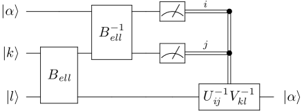
Figure 1: Quantum circuit for quantum teleportation using the Bell transform, as a diagrammatical representation of the teleportation equation (97) in terms of the teleportation operator (87). The diagram is read from the left to the right. The single lines denote qubits and the double lines denote classical bits. The box $B_{\textit{ell}}$ (or $B^{-1}_{\textit{ell}}$) denotes a two-qubit gate as the Bell transform $B_{\textit{ell}}$ (or its inverse $B^{-1}_{\textit{ell}}$). Alice has an unknown qubit state $|\alpha\rangle$ and wants to transfer it to Bob, and she makes the Bell measurements on her two-qubit state with the measurement outputs $(i,j)$. When Bob gets the two-bit message $(i,j)$ from Alice, he performs the local unitary correction operator $U_{\textit{ij}}^{-1}V_{\textit{kl}}^{-1}$ on his quantum state to obtain $|\alpha\rangle$. Note that the examples for $U_{\textit{ij}}$ and $V_{\textit{kl}}$ are shown in Table 6.

With the Bell transform $C_{H}$ (14), the teleportation equation (82) has the form given by

$$(1\!\!1_{2}\otimes C_{H})|\alpha\rangle|00\rangle=(C_{H}\otimes 1\!\!1_{2})\frac{1}{2}\sum_{i,j=0}^{1}|ij\rangle\widetilde{W}_{\textit{ij}}|\alpha\rangle,$$ (85)

and it has the other more meaningful form

$$(C_{H}^{-1}\otimes 1\!\!1_{2})(1\!\!1_{2}\otimes C_{H})|\alpha\rangle|00\rangle=\frac{1}{2}\sum_{i,j=0}^{1}|ij\rangle\widetilde{W}_{\textit{ij}}|\alpha\rangle,$$ (86)

in which $1\!\!1_{2}\otimes C_{H}$ represents an operation of creating the Bell state $|\Psi\rangle$ and $C_{H}^{-1}\otimes 1\!\!1_{2}$ is associated with an operation of performing Bell measurements. After Alice informs Bob the classical two bits $(i,j)$, Bob performs the local unitary correction operator $\widetilde{W}^{\dagger}_{\textit{ij}}$ on his qubit to obtain the transmitted qubit $|\alpha\rangle$.

5.3 Quantum teleportation using the Bell transform

$B_{\textit{ell}}$	$U_{\textit{ij}}$	$V_{\textit{kl}}$
$C_{H}$	$X^{j}Z^{i}$	$X^{l}Z^{k}$
$Q$	$(-\sqrt{-1})^{j}X^{i+j}Z^{i}$	$(\sqrt{-1})^{l}X^{k+l}Z^{k}$
$B$	$Z^{j+1}X^{i+j}$	$Z^{l+1}X^{k+l}$
$R$	$(\sqrt{-1})^{j}Z^{i}X^{i+j}$	$(-\sqrt{-1})^{l}Z^{k}X^{k+l}$

Table 6: Local unitary operators $U_{\textit{ij}}$ and $V_{\textit{kl}}$ with $i,j=0,1$ and $k,l=0,1$ in the teleportation equation (97) (or in Figure 1) for the Bell transforms $B_{\textit{ell}}=C_{H},B,Q,R$. Here $i+j$ is the binary addition modulo 2. The local unitary operators $U_{\textit{ij}}$ and $V_{\textit{kl}}$ for the Bell transforms $C_{H}$ and $Q$ have the form of products of the Pauli matrix $X$ and the Pauli matrix $Z$, while for the Bell transforms $B$ and $R$ have of the Pauli matrix $Z$ and the Pauli matrix $X$. The symbol $\sqrt{-1}$ is used to denote the imaginary unit because the symbol $i$ has been used as an index.

Through the teleportation equation (86), we realize that the operator $(C_{H}^{-1}\otimes 1\!\!1_{2})(1\!\!1_{2}\otimes C_{H})$ plays the key role in the algebraic formulation of quantum teleportation, so we propose the concept of the teleportation operator given by

$$(B^{-1}_{\textit{ell}}\otimes 1\!\!1_{2})(1\!\!1_{2}\otimes B_{\textit{ell}}),$$ (87)

or given by

$$(1\!\!1_{2}\otimes B^{-1}_{\textit{ell}})(B_{\textit{ell}}\otimes 1\!\!1_{2}),$$ (88)

in terms of the Bell transform $B_{\textit{ell}}$ (69), its inverse $B^{-1}_{\textit{ell}}$ and the identity operator $1\!\!1_{2}$. In the following, we derive the teleportation equations using the above teleportation operators.

Using the formula (4), the teleportation equation (82) has a generalized form

$$|\alpha\rangle\otimes|\psi(k,l)\rangle=\frac{1}{2}\sum_{i,j=0}^{1}|\psi(i,j)\rangle\otimes\widetilde{W}_{\textit{kl}}\widetilde{W}_{\textit{ij}}|\alpha\rangle,$$ (89)

which is reformulated with the Bell transform (65) as

$$(1\!\!1_{2}\otimes B_{\textit{ell}})|\alpha\rangle\otimes e^{-i\phi_{\textit{kl}}}|k^{\prime}l^{\prime}\rangle=(B_{\textit{ell}}\otimes 1\!\!1_{2})\frac{1}{2}\sum_{i,j=0}^{1}e^{-i\phi_{\textit{ij}}}|i^{\prime}j^{\prime}\rangle\otimes\widetilde{W}_{\textit{kl}}\widetilde{W}_{\textit{ij}}|\alpha\rangle.$$ (90)

Such the equation has a further simplified form,

$$(B^{-1}_{\textit{ell}}\otimes 1\!\!1_{2})(1\!\!1_{2}\otimes B_{\textit{ell}})|\alpha\rangle\otimes|k^{\prime}l^{\prime}\rangle=\frac{1}{2}\sum_{i,j=0}^{1}|i^{\prime}j^{\prime}\rangle\otimes\widetilde{V}_{\textit{kl}}\widetilde{U}_{\textit{ij}}|\alpha\rangle,$$ (91)

where two single-qubit gates $\widetilde{V}_{\textit{kl}}$ and $\widetilde{U}_{\textit{ij}}$ have the form

$$\widetilde{V}_{\textit{kl}}=e^{i\phi_{\textit{kl}}}\widetilde{W}_{\textit{kl}},\quad\widetilde{U}_{\textit{ij}}=e^{-i\phi_{\textit{ij}}}\widetilde{W}_{\textit{ij}},$$ (92)

and the indices $i$, $j$, $k$ and $l$ are bijective functions of $i^{\prime}$, $j^{\prime}$, $k^{\prime}$ and $l^{\prime}$, respectively, given by

$$i=f(i^{\prime},j^{\prime}),\quad j=g(i^{\prime},j^{\prime}),\quad k=f(k^{\prime},l^{\prime}),\quad l=g(k^{\prime},l^{\prime}).$$ (93)

For notational convenience, we rewrite (91) as

$$(B^{-1}_{\textit{ell}}\otimes 1\!\!1_{2})(1\!\!1_{2}\otimes B_{\textit{ell}})|\alpha\rangle\otimes|kl\rangle=\frac{1}{2}\sum_{i,j=0}^{1}|ij\rangle\otimes\widetilde{V}_{\textit{k}^{\prime}\textit{l}^{\prime}}\widetilde{U}_{\textit{i}^{\prime}\textit{j}^{\prime}}|\alpha\rangle,$$ (94)

in which the bijective mappings between lower indices are given by

$$i^{\prime}=f(i,j),\quad j^{\prime}=g(i,j),\quad k^{\prime}=f(k,l),\quad l^{\prime}=g(k,l),$$ (95)

with functions $f$ and $g$ defined in (93). Furthermore, with the notations $V_{\textit{kl}}$ and $U_{\textit{ij}}$, respectively defined by

$$V_{\textit{kl}}=\widetilde{V}_{\textit{k}^{\prime}\textit{l}^{\prime}},\quad U_{\textit{ij}}=\widetilde{U}_{\textit{i}^{\prime}\textit{j}^{\prime}},$$ (96)

we have an appropriate form of the teleportation equation given by

$$(B^{-1}_{\textit{ell}}\otimes 1\!\!1_{2})(1\!\!1_{2}\otimes B_{\textit{ell}})|\alpha\rangle|kl\rangle=\frac{1}{2}\sum_{i,j=0}^{1}|ij\rangle V_{\textit{kl}}U_{\textit{ij}}|\alpha\rangle,$$ (97)

with $k,l=0,1$, which is to be exploited in the following study.

We draw Figure 1 as a diagrammatical representation of the teleportation equation (97) in terms of the teleportation operator (87). As a matter of fact, it is the quantum circuit model of quantum teleportation, in which Bob performs the local unitary operation $U_{\textit{ij}}^{-1}V_{\textit{kl}}^{-1}$ on his qubit to obtain the transmitted qubit $|\alpha\rangle$. For example, when the Bell transform $B_{\textit{ell}}$ is the $C_{H}$ gate, the Yang–Baxter gate $B$, the matchgate $Q$ and the parity-preserving gate $R$ in Section 2, the explicit forms of the associated single-qubit gates $U_{\textit{ij}}$ and $V_{\textit{kl}}$ are collected in Table 6.

Note that the phase factors of the single-qubit gates $V_{\textit{kl}}$ and $U_{\textit{ij}}$ (92) and (96) originally come from the phase gate $E$ (68) in the matrix formulation of the Bell transform (69). In view of the teleportation equation (97), both the unitary correction operators $(V_{\textit{kl}}U_{\textit{ij}})^{\dagger}$ and $(\widetilde{W}_{\textit{kl}}\widetilde{W}_{\textit{ij}})^{\dagger}$ in quantum teleportation give rise to the same qubit state $|\alpha\rangle$ modulo a global phase. Hence, the phase gate $E$ does not play physical roles in view of the performance of quantum teleportation. On the other hand, the phase gate $E$ makes sense in quantum computation. Usually, the phase gate $E$ is not a Clifford gate, for example, $E=T\otimes 1\!\!1_{2}$ with the $T$ gate (9), refer to Subsection 4.3. Therefore the quantum circuit of teleportation can be regarded as quantum non-Clifford gate computation.

To derive another form of the teleportation equation using the teleportation operator (88), we start from the teleportation equation expressed as

$$|\Psi\rangle\otimes|\alpha\rangle=\frac{1}{2}\sum_{i,j=0}^{1}\widetilde{W}^{T}_{\textit{ij}}|\alpha\rangle\otimes|\psi(i,j)\rangle,$$ (98)

and then exploit the following property of the Bell states (4),

$$|\psi(k,l)\rangle=(\widetilde{W}^{T}_{\textit{kl}}\otimes 1\!\!1_{2})|\Psi\rangle,$$ (99)

to obtain the teleportation equation

$$(1\!\!1_{2}\otimes B^{-1}_{\textit{ell}})(B_{\textit{ell}}\otimes 1\!\!1_{2})|kl\rangle|\alpha\rangle=\frac{1}{2}\sum_{i,j=0}^{1}V^{T}_{\textit{kl}}U^{T}_{\textit{ij}}|\alpha\rangle|ij\rangle,$$ (100)

which is to be used in the fault-tolerant construction of two-qubit gates in teleportation-based quantum computation, refer to Figure 3 in Subsection 6.2.

5.4 The diagrammatical representation of the Bell transform

In view of the recent research [19] which shows that the quantum circuit model of teleportation admits a nice topological diagrammatical representation, we study the topological diagrammatical representation of the teleportation operator (87) or (88), which provides a simpler diagrammatical proof for deriving the teleportation equation (97) or (100). In the following, only specific diagrammatical rules [19] are reviewed just enough for the present usage in this subsection (The complete set of diagrammatical rules is referred to [19]).

With the single-qubit gate $V_{\textit{kl}}$ (96), the Bell transform (66) can be expressed as

$$B_{\textit{ell}}=\sum_{k,l=0}^{1}e^{i\phi_{\textit{k}^{\prime}\textit{l}^{\prime}}}|\psi(k^{\prime},l^{\prime})\rangle\langle kl|=\sum_{k,l=0}^{1}(1\!\!1_{2}\otimes V_{\textit{kl}})|\Psi\rangle\langle kl|.$$ (101)

In view of the diagrammatical rules [19], a single vertical line with the symbol $\triangle$ denotes a covector product state $\langle 0|$, and the one with the action of the Pauli gate $X$ stands for the state $\langle 1|$; a solid point on the configuration denotes a single-qubit gate; a cup configuration represents the Bell state $|\Psi\rangle$. The diagrammatical representation of the Bell transform (66) is pictured as

$$\begin{array}[]{c}\begin{picture}(80.0,30.0)\par\put(3.0,14.0){$B_{\textit{ell}}=\sum_{k,l=0}^{1}$} \par\put(54.0,18.0){\line(0,1){12.0}} \put(44.0,18.0){\line(0,1){12.0}} \put(44.0,18.0){\line(1,0){10.0}} \put(54.0,24.0){\circle*{2.0}} \put(56.0,23.0){\tiny{$V_{\textit{kl}}$}} \par\put(44.0,0.0){\line(0,1){10.0}} \put(54.0,0.0){\line(0,1){10.0}} \put(54.0,6.0){\circle*{2.0}} \put(55.0,5.0){\tiny{$X^{l}$}} \put(44.0,6.0){\circle*{2.0}} \put(45.0,5.0){\tiny{$X^{k}$}} \par\put(42.3,10.0){\tiny{$\triangle$}} \put(52.3,10.0){\tiny{$\triangle$}} \par\end{picture}\end{array},$$ (102)

in which the diagrammatical representation is read from the bottom to the top and its associated algebraical expression (101) is read from the right to the left.

With the single-qubit gate $U_{\textit{ij}}$ (96), the inverse of the Bell transform (66) has the form

$$B^{-1}_{\textit{ell}}=\sum_{i,j=0}^{1}|ij\rangle\langle\psi(i^{\prime},j^{\prime})|e^{-i\phi_{\textit{i}^{\prime}\textit{j}^{\prime}}}=\sum_{i,j=0}^{1}|ij\rangle\langle\Psi|(1\!\!1_{2}\otimes U^{T}_{\textit{ij}}).$$ (103)

In accordance with the diagrammatical rules [19], a cap configuration denotes the complex conjugation of the Bell state $|\Psi\rangle$ and a vertical line with the symbol $\nabla$ denotes the state $|0\rangle$. The inverse of the Bell transform (66) has the following diagrammatical representation

$$\begin{array}[]{c}\begin{picture}(80.0,30.0)\par\put(3.0,14.0){$B^{-1}_{\textit{ell}}=\sum_{i,j=0}^{1}$} \par\put(54.0,20.0){\line(0,1){10.0}} \put(44.0,20.0){\line(0,1){10.0}} \put(54.0,24.0){\circle*{2.0}} \put(55.0,23.0){\tiny{$X^{j}$}} \put(44.0,24.0){\circle*{2.0}} \put(45.0,23.0){\tiny{$X^{i}$}} \par\put(42.3,18.0){\tiny{$\nabla$}} \put(52.3,18.0){\tiny{$\nabla$}} \par\put(44.0,0.0){\line(0,1){12.0}} \put(54.0,0.0){\line(0,1){12.0}} \put(44.0,12.0){\line(1,0){10.0}} \put(54.0,6.0){\circle*{2.0}} \put(55.9,5.0){\tiny{$U^{T}_{\textit{ij}}$}} \par\end{picture}\end{array},$$ (104)

which is read from the bottom to the top.

With the help of the diagrammatical representations (102) and (104), the teleportation operator (87) has the diagrammatical representation

$$\begin{array}[]{c}\begin{picture}(30.0,65.0)\par\put(-110.0,29.0){$(B^{-1}_{\textit{ell}}\otimes 1\!\!1_{2})(1\!\!1_{2}\otimes B_{\textit{ell}})=\sum_{i,j,k,l=0}^{1}$} \par\put(14.5,48.0){\line(0,1){12.0}} \put(2.0,48.0){\line(0,1){12.0}} \put(14.5,54.0){\circle*{2.0}} \put(15.5,53.0){\tiny{$X^{j}$}} \put(2.0,54.0){\circle*{2.0}} \put(3.0,53.0){\tiny{$X^{i}$}} \par\put(-0.2,45.0){{\scriptsize$\nabla$}} \put(12.3,45.0){\scriptsize{$\nabla$}} \par\put(14.5,30.0){\circle*{2.0}} \put(16.0,29.0){\tiny{$U^{T}_{\textit{ij}}$}} \par\put(14.5,0.0){\line(0,1){12.0}} \put(27.0,0.0){\line(0,1){12.0}} \put(27.0,6.0){\circle*{2.0}} \put(28.0,5.0){\tiny{$X^{l}$}} \put(14.5,6.0){\circle*{2.0}} \put(15.5,5.0){\tiny{$X^{k}$}} \par\put(12.3,12.0){\tiny{$\triangle$}} \put(24.8,12.0){\tiny{$\triangle$}} \par\put(2.0,0.0){\line(0,1){37.5}} \put(2.0,37.5){\line(1,0){12.5}} \put(14.5,22.5){\line(0,1){15.0}} \put(27.0,22.5){\line(0,1){37.5}} \put(14.5,22.5){\line(1,0){12.5}} \par\put(27.0,30.0){\circle*{2.0}} \put(28.5,29.0){\tiny{$V_{\textit{kl}}$}} \par\put(42.0,29.0){$=\sum_{i,j,k,l=0}^{1}$} \par\put(94.5,48.0){\line(0,1){12.0}} \put(82.0,48.0){\line(0,1){12.0}} \put(94.5,54.0){\circle*{2.0}} \put(95.5,53.0){\tiny{$X^{j}$}} \put(82.0,54.0){\circle*{2.0}} \put(83.0,53.0){\tiny{$X^{i}$}} \par\put(79.8,45.0){{\scriptsize$\nabla$}} \put(92.3,45.0){\scriptsize{$\nabla$}} \par\par\put(94.5,0.0){\line(0,1){12.0}} \put(107.0,0.0){\line(0,1){12.0}} \put(107.0,6.0){\circle*{2.0}} \put(108.0,5.0){\tiny{$X^{l}$}} \put(94.5,6.0){\circle*{2.0}} \put(95.5,5.0){\tiny{$X^{k}$}} \par\put(92.3,12.0){\tiny{$\triangle$}} \put(104.8,12.0){\tiny{$\triangle$}} \par\put(82.0,0.0){\line(0,1){37.5}} \put(82.0,37.5){\line(1,0){12.5}} \put(94.5,22.5){\line(0,1){15.0}} \put(107.0,22.5){\line(0,1){37.5}} \put(94.5,22.5){\line(1,0){12.5}} \par\put(107.0,54.0){\circle*{2.0}} \put(108.5,53.0){\tiny{$V_{\textit{kl}}U_{\textit{ij}}$}} \par\end{picture}\end{array}$$ (105)

in which the diagrammatical rules [19] are exploited: the vertical line represents the identity operator $1\!\!1_{2}$ and the single-qubit gate $U^{T}_{\textit{ij}}$ flows from one branch to the adjacent branch with the transpose operation. To derive the teleportation equation (97) in a diagrammatical approach, we apply the teleportation operator (87) on the prepared state $|\alpha\rangle|kl\rangle$ and then straighten the connected line of the top cap with the bottom cup as a sort of topological deformation, so that the unknown qubit $|\alpha\rangle$ with the action of the local unitary operation $V_{\textit{kl}}U_{\textit{ij}}$ is transmitted.

To complete the study of the diagrammatical representation of the teleportation operator, we draw the associated configuration of the teleportation operator (88) as

$$\begin{array}[]{c}\begin{picture}(30.0,65.0)\par\put(-110.0,29.0){$(1\!\!1_{2}\otimes B^{-1}_{\textit{ell}})(B_{\textit{ell}}\otimes 1\!\!1_{2})=\sum_{i,j,k,l=0}^{1}$} \par\put(14.5,48.0){\line(0,1){12.0}} \put(27.0,48.0){\line(0,1){12.0}} \put(14.5,54.0){\circle*{2.0}} \put(15.5,53.0){\tiny{$X^{i}$}} \put(27.0,54.0){\circle*{2.0}} \put(29.5,53.0){\tiny{$X^{j}$}} \par\put(24.8,45.0){{\scriptsize$\nabla$}} \put(12.3,45.0){\scriptsize{$\nabla$}} \par\put(14.5,30.0){\circle*{2.0}} \put(16.0,29.0){\tiny{$V_{\textit{kl}}$}} \par\put(14.5,0.0){\line(0,1){12.0}} \put(2.0,0.0){\line(0,1){12.0}} \put(2.0,6.0){\circle*{2.0}} \put(15.5,5.0){\tiny{$X^{l}$}} \put(14.5,6.0){\circle*{2.0}} \put(3.0,5.0){\tiny{$X^{k}$}} \par\put(12.3,12.0){\tiny{$\triangle$}} \put(-0.2,12.0){\tiny{$\triangle$}} \par\put(27.0,0.0){\line(0,1){37.5}} \put(2.0,22.5){\line(1,0){12.5}} \put(14.5,22.5){\line(0,1){15.0}} \put(2.0,22.5){\line(0,1){37.5}} \put(14.5,37.5){\line(1,0){12.5}} \par\put(27.0,30.0){\circle*{2.0}} \put(28.5,29.0){\tiny{$U^{T}_{\textit{ij}}$}} \par\put(41.0,29.0){$=\sum_{i,j,k,l=0}^{1}$} \par\put(94.5,48.0){\line(0,1){12.0}} \put(107.0,48.0){\line(0,1){12.0}} \put(94.5,54.0){\circle*{2.0}} \put(95.5,53.0){\tiny{$X^{i}$}} \put(107.0,54.0){\circle*{2.0}} \put(108.0,53.0){\tiny{$X^{j}$}} \par\put(104.8,45.0){{\scriptsize$\nabla$}} \put(92.3,45.0){\scriptsize{$\nabla$}} \par\par\put(94.5,0.0){\line(0,1){12.0}} \put(82.0,0.0){\line(0,1){12.0}} \put(82.0,6.0){\circle*{2.0}} \put(83.0,5.0){\tiny{$X^{k}$}} \put(94.5,6.0){\circle*{2.0}} \put(95.5,5.0){\tiny{$X^{l}$}} \par\put(92.3,12.0){\tiny{$\triangle$}} \put(79.8,12.0){\tiny{$\triangle$}} \par\put(107.0,0.0){\line(0,1){37.5}} \put(82.0,22.5){\line(1,0){12.5}} \put(94.5,22.5){\line(0,1){15.0}} \put(82.0,22.5){\line(0,1){37.5}} \put(94.5,37.5){\line(1,0){12.5}} \par\put(82.0,54.0){\circle*{2.0}} \put(64.0,53.0){\tiny{$V^{T}_{\textit{kl}}U^{T}_{\textit{ij}}$}} \par\par\end{picture}\end{array}$$ (106)

which naturally gives rise to the teleportation equation (100).

6 Teleportation-based quantum computation using the Bell transform

Teleportation-based quantum computation has been well studied in both algebraic and topological approach in [16, 17, 18, 19]. Here we present a brief review on the fault-tolerant construction of single-qubit gates and two-qubit gates using quantum teleportation, and then make a study on the fault-tolerant construction of the universal quantum gate set in teleportation-based quantum computation using the Bell transform.

6.1 Review on teleportation-based quantum computation

In quantum information and computation [1], quantum gates $U$ are classified by

$$C_{k}\equiv\{U|UC_{k-2}U^{\dagger}\subseteq C_{k-1}\},$$ (107)

where $C_{1}$ denotes the Pauli gates and $C_{2}$ denotes the Clifford gates. In fault-tolerant quantum computation [1, 2, 22], the fault-tolerant construction of Clifford gates including the Pauli gates can be performed in a systematical approach, and the fault-tolerant construction of non-Clifford gates such as the $T$ gate (9) becomes a problem of how to introduce a set of Clifford gates to play the role of these non-Clifford gates. Teleportation-based quantum computation [16] is fault-tolerant quantum computation because it fault-tolerantly prepares a quantum state with the action of a $C_{3}$ gate and then fault-tolerantly applies $C_{1}$ or $C_{2}$ gates to such the quantum state using the teleportation protocol so that this $C_{3}$ gate can be fault-tolerantly performed.

To fault-tolerantly perform a single-qubit gate $U\in C_{k}$ (107) on the unknown qubit state $|\alpha\rangle$, Alice prepares the two-qubit state $|\Psi_{U}\rangle$ given by

$$|\Psi_{U}\rangle=(1\!\!1_{2}\otimes U)|\Psi\rangle,$$ (108)

and expresses $|\alpha\rangle\otimes|\Psi_{U}\rangle$ as

$$|\alpha\rangle\otimes|\Psi_{U}\rangle=\frac{1}{2}\sum_{i,j=0}^{1}|\psi(ij)\rangle\otimes R_{\textit{ij}}U|\alpha\rangle,$$ (109)

where the single-qubit gate $R_{\textit{ij}}$ has the form $R_{\textit{ij}}=U\widetilde{W}_{\textit{ij}}U^{\dagger}\in C_{k-1}$ (107). Then Alice makes Bell measurements $|\psi(ij)\rangle\langle\psi(ij)|\otimes 1\!\!1_{2}$ and informs Bob her measurement results labeled by $(i,j)$. Finally, Bob performs the unitary correction operator $R_{\textit{ij}}^{\dagger}\in C_{k-1}$ to attain $U|\alpha\rangle$. It is obvious that the difficulty of fault-tolerantly performing the single-qubit gate $U\in C_{k}$ becomes how to fault-tolerantly prepare the state $|\Psi_{U}\rangle$ and perform the single-qubit gate $R_{\textit{ij}}^{\dagger}\in C_{k-1}$.

To fault-tolerantly perform a two-qubit gate CU on two unknown single-qubit states $|\alpha\rangle$ and $|\beta\rangle$, we prepare a four-qubit entangled state $|\Psi_{\textit{CU}}\rangle$ given by

$$|\Psi_{\textit{CU}}\rangle=(1\!\!1_{2}\otimes\textit{CU}\otimes 1\!\!1_{2})(|\Psi\rangle\otimes|\Psi\rangle),$$ (110)

with the action of the CU gate, and reformulate the prepared state $|\alpha\rangle\otimes|\Psi_{CU}\rangle\otimes|\beta\rangle$ as

$$\begin{split}&|\alpha\rangle\otimes|\Psi_{\textit{CU}}\rangle\otimes|\beta\rangle\\ =&\frac{1}{4}\sum_{i_{1},j_{1}=0}^{1}\sum_{i_{2},j_{2}=0}^{1}(1\!\!1_{4}\otimes Q\otimes P\otimes 1\!\!1_{4})(|\psi(i_{1}j_{1})\rangle\otimes\textit{CU}|\alpha\beta\rangle\otimes|\psi(i_{2}j_{2})\rangle),\end{split}$$ (111)

with $1\!\!1_{4}=1\!\!1_{2}\otimes 1\!\!1_{2}$. The single-qubit gates $Q$ and $P$ in the teleportation equation (111) are calculated by

$$Q\otimes P=\textit{CU}(\widetilde{W}_{\textit{i}_{1}\textit{j}_{1}}\otimes\widetilde{W}^{T}_{\textit{i}_{2}\textit{j}_{2}})\textit{CU}^{\dagger},$$ (112)

which informs that the $Q$ and $P$ gates (112) are single-qubit Pauli gates when the CU gate is a Clifford gate [1, 22]. Next, we perform the Bell measurements given by

$$|\psi(i_{1}j_{1})\rangle\langle\psi(i_{1}j_{1})|\otimes 1\!\!1_{2}\otimes 1\!\!1_{2}\otimes|\psi(i_{2}j_{2})\rangle\langle\psi(i_{2}j_{2})|,$$ (113)

and with the measurement results labeled by $(i_{1},j_{1})$ and $(i_{2},j_{2})$, we perform the unitary correction operator, $Q^{\dagger}\otimes P^{\dagger}$, to obtain the exact action of the CU gate on the two-qubit state $|\alpha\rangle\otimes|\beta\rangle$, namely $\textit{CU}|\alpha\beta\rangle$. Note that the two-qubit gate CU we study here may not be a controlled-operation two-qubit gate such as the CNOT gate.

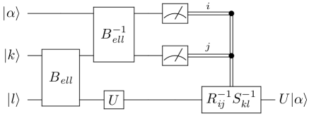
Figure 2: Fault-tolerant construction of the single-qubit gate $U$ in teleportation-based quantum computation using the Bell transform, as a diagrammatical representation of the teleportation equation (115) in terms of the teleportation operator (87). Alice prepares an unknown qubit state $|\alpha\rangle$ and shares with Bob a two-qubit state with the local action of the $U$ gate, and Alice makes the Bell measurements on her two-qubit system with the measurement outputs $(i,j)$. When Bob gets the two-bit message $(i,j)$ from Alice, he performs the local unitary correction operator $R^{-1}_{\textit{ij}}S_{\textit{kl}}^{-1}$ on his qubit to obtain the qubit state $U|\alpha\rangle$. Note that the examples for the $R_{\textit{ij}}$ and $S_{\textit{kl}}$ gates are shown in Table 7 and Table 8.

$B_{\textit{ell}}$	$U$	$R_{\textit{ij}}$	$S_{\textit{kl}}$
$C_{H}$		$Z^{j}X^{i}$	$Z^{l}X^{k}$
$B$		$X^{j+1}Z^{i+j}$	$X^{l+1}Z^{k+l}$
$Q$	$H$	$(-\sqrt{-1})^{j}Z^{i+j}X^{i}$	$(\sqrt{-1})^{l}Z^{k+l}X^{k}$
$R$		$(\sqrt{-1})^{j}X^{i}Z^{i+j}$	$(-\sqrt{-1})^{l}X^{k}Z^{k+l}$

Table 7: Local unitary operators $R_{\textit{ij}}$ and $S_{\textit{kl}}$ with $i,j=0,1$ and $k,l=0,1$ in the teleportation equation (115) (or in Figure 2) for the Bell transforms $B_{\textit{ell}}=C_{H},B,Q,R$ with the single-qubit gate $U$ as the Hadamard gate $H$.

$B_{\textit{ell}}$	$U$	$R_{\textit{ij}}$	$S_{\textit{kl}}$
$C_{H}$		$W^{j}Z^{i}$	$W^{l}Z^{k}$
$B$		$Z^{j+1}W^{i+j}$	$Z^{l+1}W^{k+l}$
$Q$	$T$	$(-\sqrt{-1})^{j}W^{i+j}Z^{i}$	$(\sqrt{-1})^{l}W^{k+l}Z^{k}$
$R$		$(\sqrt{-1})^{j}Z^{i}W^{i+j}$	$(-\sqrt{-1})^{l}Z^{k}W^{k+l}$

Table 8: Local unitary operators $R_{\textit{ij}}$ and $S_{\textit{kl}}$ with $i,j=0,1$ and $k,l=0,1$ in the teleportation equation (115) (or in Figure 2) for the Bell transforms $B_{\textit{ell}}=C_{H},B,Q,R$ with the single-qubit gate $U$ as the $T$ gate. Note that the single-qubit gate $W$ is the Clifford gate (11).

6.2 Teleportation-based quantum computation using the Bell transform

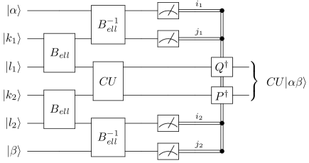
Figure 3: Fault-tolerant construction of the two-qubit gate CU in teleportation-based quantum computation using the Bell transform, as a diagrammatical representation of the teleportation equation (6.2). We prepare an unknown two-qubit state $|\alpha\beta\rangle$ and a four-qubit state with the action of the two-qubit gate CU, and perform the joint Bell measurements with the measurement outputs $(i_{1},j_{1})$ and $(i_{2},j_{2})$. With these two-bit messages, we perform the unitary correction operator $Q^{\dagger}\otimes P^{\dagger}$ to obtain $|\alpha\beta\rangle$ with the action of the CU gate. Note that the examples for the $Q$ and $P$ gates are shown in Table 9 and Table 10.

$B_{\textit{ell}}$	CU	$Q$	$P$
	CNOT	$E_{Q}X^{a}Z^{b}Z^{c}$	$E_{P}X^{a}Z^{c}X^{d}$
	CZ	$E_{Q}X^{a}Z^{b}Z^{d}$	$E_{P}Z^{a}Z^{c}X^{d}$
	$C_{H}$	$E_{Q}Z^{a}X^{b}Z^{c}$	$E_{P}X^{b}Z^{c}X^{d}$
	$C_{H}^{-1}$	$E_{Q}Z^{a}X^{b}X^{c}$	$E_{P}X^{a}Z^{c}X^{d}$
	$B$	$(-1)^{b}E_{Q}X^{a}Y^{b}X^{c}X^{d}$	$(-1)^{c}E_{P}Y^{b}X^{c}Z^{d}$
$C_{H}/Q$	$B^{-1}$	$E_{Q}X^{a}Y^{b}X^{c}X^{d}$	$(-1)^{d}E_{P}Y^{b}X^{c}Z^{d}$
	$Q$	$E_{Q}Z^{a}X^{b}Y^{c}Y^{d}$	$(-\sqrt{-1})^{d}E_{P}X^{a}X^{b}Y^{c}Z^{d}$
	$Q^{-1}$	$(\sqrt{-1})^{a}(\sqrt{-1})^{b}E_{Q}Z^{a}X^{b}Y^{c}$	$(\sqrt{-1})^{c}(\sqrt{-1})^{d}E_{P}Y^{a}Y^{b}X^{c}Y^{d}$
	$R$	$E_{Q}X^{a}X^{b}Y^{c}Z^{d}$	$(\sqrt{-1})^{d}E_{P}Z^{a}X^{b}Y^{c}Y^{d}$
	$R^{-1}$	$(-\sqrt{-1})^{a}(-\sqrt{-1})^{b}E_{Q}Y^{b}X^{c}Z^{d}$	$(-\sqrt{-1})^{c}(-\sqrt{-1})^{d}E_{P}Y^{a}X^{b}Y^{c}Y^{d}$

Table 9: Local unitary operators $Q$ and $P$ in the teleportation equation (6.2) (or in Figure 3), with the teleportation operator (87) in terms of the Bell transforms $C_{H}$ and $Q$, for two-qubit gates CU including the CNOT gate, the CZ gate, the Bell transforms $B_{\textit{ell}}=C_{H},B,Q,R$ and their inverses. The local unitary gates $Q$ and $P$ have the forms as products of the Pauli matrices $X$ and $Z$, with respective indices $a,b,c,d$ in Table 11 and respective phase factors $E_{Q}$ and $E_{P}$ in Table 12. Note that the $Y$ gate is defined in (12).

$B_{\textit{ell}}$	CU	$Q$	$P$
	CNOT	$E_{Q}Z^{a}X^{b}Z^{d}$	$E_{P}X^{b}X^{c}Z^{d}$
	CZ	$E_{Q}Z^{a}X^{b}Z^{c}$	$E_{P}Z^{b}X^{c}Z^{d}$
	$C_{H}$	$E_{Q}X^{a}Z^{b}Z^{d}$	$E_{P}X^{a}X^{c}Z^{d}$
	$C_{H}^{-1}$	$E_{Q}X^{a}Z^{b}X^{d}$	$E_{P}X^{b}X^{c}Z^{d}$
	$B$	$(-1)^{a}E_{Q}Y^{a}X^{b}X^{c}X^{d}$	$(-1)^{d}E_{P}Y^{a}Z^{c}X^{d}$
$B/R$	$B^{-1}$	$E_{Q}Y^{a}X^{b}X^{c}X^{d}$	$(-1)^{c}E_{P}Y^{a}Z^{c}X^{d}$
	$Q$	$E_{Q}X^{a}Z^{b}Y^{c}Y^{d}$	$(-\sqrt{-1})^{c}E_{P}X^{a}X^{b}Z^{c}Y^{d}$
	$Q^{-1}$	$(\sqrt{-1})^{a}(\sqrt{-1})^{b}E_{Q}X^{a}Z^{b}Y^{d}$	$(\sqrt{-1})^{c}(\sqrt{-1})^{d}E_{P}Y^{a}Y^{b}Y^{c}X^{d}$
	$R$	$E_{Q}X^{a}X^{b}Z^{c}Y^{d}$	$(\sqrt{-1})^{c}E_{P}X^{a}Z^{b}Y^{c}Y^{d}$
	$R^{-1}$	$(-\sqrt{-1})^{a}(-\sqrt{-1})^{b}E_{Q}Y^{a}Z^{c}X^{d}$	$(-\sqrt{-1})^{c}(-\sqrt{-1})^{d}E_{P}X^{a}Y^{b}Y^{c}Y^{d}$

Table 10: Local unitary operators $Q$ and $P$ in the teleportation equation (6.2) (or in Figure 3), with the teleportation operator (87) in terms of the Bell transforms $B$ and $R$, for two-qubit gates CU including the CNOT gate, the CZ gate, the Bell transforms $B_{\textit{ell}}=C_{H},B,Q,R$ and their inverses. Indices $a,b,c,d$ are shown in Table 11, and phase factors $E_{Q}$ and $E_{P}$ are in Table 12.

	$a$	$b$	$c$	$d$
$C_{H}$	$j_{1}+l_{1}$	$i_{1}+k_{1}$	$i_{2}+k_{2}$	$j_{2}+l_{2}$
$B$	$j_{1}+l_{1}$	$i_{1}+j_{1}+k_{1}+l_{1}$	$i_{2}+j_{2}+k_{2}+l_{2}$	$j_{2}+l_{2}$
$Q$	$i_{1}+j_{1}+k_{1}+l_{1}$	$i_{1}+k_{1}$	$i_{2}+k_{2}$	$i_{2}+j_{2}+k_{2}+l_{2}$
$R$	$i_{1}+k_{1}$	$i_{1}+j_{1}+k_{1}+l_{1}$	$i_{2}+j_{2}+k_{2}+l_{2}$	$i_{2}+k_{2}$

Table 11: The indices $a,b,c,d$ for the Bell transforms $B_{\textit{ell}}=C_{H},Q$ in Table 9 and the Bell transforms $B_{\textit{ell}}=B,R$ in Table 10. All the index addition $+$ is the binary addition.

	$E_{Q}$	$E_{P}$
$C_{H}$	$(-1)^{j_{1}\cdot k_{1}}$	$(-1)^{i_{2}\cdot l_{2}}$
$B$	$(-1)^{(k_{1}+l_{1})\cdot(j_{1}+1)}$	$(-1)^{(i_{2}+j_{2})\cdot(l_{2}+1)}$
$Q$	$(-1)^{(i_{1}+j_{1})\cdot k_{1}}(-\sqrt{-1})^{j_{1}}(\sqrt{-1})^{l_{1}}$	$(-1)^{(k_{2}+l_{2})\cdot i_{2}}(-\sqrt{-1})^{j_{2}}(\sqrt{-1})^{l_{2}}$
$R$	$(-1)^{(k_{1}+l_{1})\cdot i_{1}}(-\sqrt{-1})^{l_{1}}(\sqrt{-1})^{j_{1}}$	$(-1)^{(i_{2}+j_{2})\cdot k_{2}}(-\sqrt{-1})^{l_{2}}(\sqrt{-1})^{j_{2}}$

Table 12: The phase factors $E_{Q}$ and $E_{P}$ for the Bell transforms $B_{\textit{ell}}=C_{H},Q$ in Table 9 and the Bell transforms $B_{\textit{ell}}=B,R$ in Table 10. All the index multiplication $\cdot$ is the logical AND operation.

We study the fault-tolerant construction of the universal quantum gate set using the teleportation operator (87) or (88). Refer to Subsection 2.2, we know that an entangling two-qubit gate with all single-qubit gates are capable of performing universal quantum computation. An entangling two-qubit Clifford gate can be any one of the CNOT gate, the CZ gate, the Bell transforms $C_{H}$, $B$, $Q$, $R$ and their inverses $C^{-1}_{H}$, $B^{-1}$, $Q^{-1}$, $R^{-1}$. Single-qubit gates can be generated by the Hadamard gate $H$ and the $T$ gate. Note that all of these quantum gates have been defined in the previous sections and in the appendix.

To perform a single-qubit gate $U$ on the unknown qubit state $|\alpha\rangle$, namely $U|\alpha\rangle$, Alice prepares the quantum state given by

$$|\alpha\rangle\otimes|\psi_{U}(k^{\prime},l^{\prime})\rangle,$$ (114)

with $|\psi_{U}(k^{\prime},l^{\prime})\rangle=(1\!\!1_{2}\otimes U)B_{\textit{ell}}|kl\rangle$ (different from $|\Psi_{U}\rangle$ (108)). Note that the bijective mappings between $k^{\prime},l^{\prime}$ and $k,l$ are defined in (95). Then Alice applies the Bell measurement denoted by $B^{-1}_{\textit{ell}}\otimes 1\!\!1_{2}$ to the prepared quantum state. These two successive operations lead to the teleportation equation given by

$$(B_{\textit{ell}}^{-1}\otimes 1\!\!1_{2})(1\!\!1_{2}\otimes 1\!\!1_{2}\otimes U)(1\!\!1_{2}\otimes B_{\textit{ell}})|\alpha\rangle|\textit{kl}\rangle=\frac{1}{2}\sum_{i,j=0}^{1}|ij\rangle S_{\textit{kl}}R_{\textit{ij}}U|\alpha\rangle,$$ (115)

with $S_{\textit{kl}}R_{\textit{ij}}=U(V_{\textit{kl}}U_{\textit{ij}})U^{\dagger}$. When Bob gets the classical two-bit message $(i,j)$ from Alice, he performs the local unitary correction operator $R_{\textit{ij}}^{-1}S_{\textit{kl}}^{-1}$ on his qubit to obtain the expected qubit state $U|\alpha\rangle$. Refer to Figure 2 for the quantum circuit associated with the teleportation equation (115).

Note that the $V_{\textit{kl}}U_{\textit{ij}}$ gate (Table 6) is a Pauli gate. As the single-qubit gate $U$ is the Hadamard gate $H$, the $S_{\textit{kl}}R_{\textit{ij}}$ gate (Table 7) is still a Pauli gate. As the $U$ gate is the $T$ gate (9), the $S_{\textit{kl}}R_{\textit{ij}}$ gate (Table 8) is a Clifford gate. Hence, the fault-tolerant procedure of performing the $T$ gate consists of two steps [16]: The first step is to fault-tolerantly prepare the state $|\psi_{U}(k^{\prime},l^{\prime})\rangle$ with $U=T$, and the second step is to fault-tolerantly perform the associated Clifford gate $R_{\textit{ij}}^{-1}S_{\textit{kl}}^{-1}$.

The fault-tolerant construction of a two-qubit gate CU depends on the fault-tolerant construction of the quantum state given by

$$|\psi_{\textit{CU}}\rangle=(1\!\!1_{2}\otimes\textit{CU}\otimes 1\!\!1_{2})(B_{\textit{ell}}\otimes B_{\textit{ell}})|k_{1}l_{1}\rangle\otimes|k_{2}l_{2}\rangle,$$ (116)

which is a four-qubit state (different from $|\Psi_{\textit{CU}}\rangle$ (110)). This state together with an unknown two-qubit product state $|\alpha\beta\rangle$ given by

$$|\alpha\rangle\otimes|\psi_{\textit{CU}}\rangle\otimes|\beta\rangle,$$ (117)

is the prepared quantum state to be used. Applying the joint Bell measurement given by

$$B^{-1}_{\textit{ell}}\otimes 1\!\!1_{2}\otimes 1\!\!1_{2}\otimes B^{-1}_{\textit{ell}},$$ (118)

to the prepared quantum state (117) gives rise to the teleportation equation

$$(B^{-1}_{\textit{ell}}\otimes 1\!\!1_{2}\otimes 1\!\!1_{2}\otimes B^{-1}_{\textit{ell}})|\alpha\rangle\otimes|\psi_{\textit{CU}}\rangle\otimes|\beta\rangle$$

$$=\frac{1}{4}\sum_{i_{1},j_{1}=0}^{1}\sum_{i_{2},j_{2}=0}^{1}(1\!\!1_{2}\otimes 1\!\!1_{2}\otimes Q\otimes P\otimes 1\!\!1_{2}\otimes 1\!\!1_{2})|i_{1}j_{1}\rangle\otimes\textit{CU}|\alpha\beta\rangle\otimes|i_{2}j_{2}\rangle,$$ (119)

with $Q\otimes P$ defined by

$$Q\otimes P=\textit{CU}(V_{\textit{k}_{1}\textit{l}_{1}}U_{\textit{i}_{1}\textit{j}_{1}}\otimes V^{T}_{\textit{k}_{2}\textit{l}_{2}}U^{T}_{\textit{i}_{2}\textit{j}_{2}})\textit{CU}^{\dagger},$$ (120)

where the teleportation equations (97) and (100) have been exploited. Hence the unitary correction operator is given by $Q^{\dagger}\otimes P^{\dagger}$. Refer to Figure 3 for the quantum circuit associated with the teleportation equation (6.2) and refer to Table 9, Table 10, Table 11 and Table 12 for the local unitary operators $Q$ and $P$ (120).

We draw Figures 1–3 and make Tables 6–12 in order to present a detailed account on the fault-tolerant construction of single-qubit gates and two-qubit gates in teleportation-based quantum computation [16, 17, 18, 19] using the Bell transform. These results show that teleportation-based computation using the Bell transform presents a platform on which quantum Clifford gate computation [1, 22], quantum matchgate computation [27, 28, 29, 30, 31], and quantum computation using the Yang–Baxter gates [24, 25] can be performed.

7 Concluding remarks

Inspired by the quantum Fourier transform [1, 2] and its application to quantum information and computation, we define the unitary basis transformation from the product basis to the GHZ basis [8, 9] as the GHZ transform, with the Bell transform as the simplest example. Since the GHZ states are widely used in quantum information sicence, we expect that the GHZ transform plays the important roles in various topics of quantum information and computation. For example, in this paper, we clearly show that the teleportation operator using the Bell transform plays a crucial role in quantum teleportation [10, 11, 12, 13, 14, 15] and teleportation-based quantum computation [16, 17, 18, 19].

The following are remarks on possible further research topics. On the Bell transform, we study its generalized form as a function of parameters, refer to the Yang–Baxter gate $B(x)$ [24, 25, 21, 36] depending on the spectral parameter $x$. On quantum teleportation, we apply the GHZ transform to multi-qubit teleportation [37, 38, 39] or quantum teleportation via non-maximally entangling resources [40, 41, 42]. There remains a natural question about the multi-qubit generalization of the teleportation operators (87) and (88). On universal quantum computation, we study topological and algebraic aspects in the one-way quantum computation [43, 44, 45] using the GHZ transform. On quantum circuit models, we try to explore interesting quantum algorithms via the GHZ transform, with the help of quantum algorithms [46, 47, 48, 49, 50] based on the quantum Fourier transform.

Notes Added. After this paper had been completed for some time, the authors have realized in their another paper [51] that it is natural and meaningful to generalize the definitions of the GHZ transform (40) (or the Bell transform (66)). The generalized GHZ transform $\widetilde{\textit{GHZ}}^{(n)}$ is defined as

$$\begin{split}\widetilde{\textit{GHZ}}^{(n)}&=\sum_{j_{1},j_{2},\ldots,j_{n}=0}^{1}\,e^{i\phi_{\textit{k}_{1}\textit{k}_{2}\ldots\textit{k}_{n}}}\,(S^{(1)}_{\textit{k}_{1}\textit{k}_{2}\ldots\textit{k}_{n}}\otimes S^{(2)}_{\textit{k}_{1}\textit{k}_{2}\ldots\textit{k}_{n}}\otimes\ldots\otimes S^{(n)}_{\textit{k}_{1}\textit{k}_{2}\ldots\textit{k}_{n}})\\ &|G(k_{1},k_{2},\ldots,k_{n})\rangle\langle j_{1},j_{2},\ldots,j_{n}|,\end{split}$$

where $k_{l}=k_{l}(j_{1},j_{2},\ldots,j_{n})$, $l=1,\ldots,n$ are bijective functions of $j_{1},j_{2},\ldots,j_{n}$; $e^{i\phi_{\textit{k}_{1}\textit{k}_{2}\ldots\textit{k}_{n}}}$ is the phase factor; and $S^{(l)}_{\textit{k}_{1}\textit{k}_{2}\ldots\textit{k}_{n}}$, $l=1,\ldots,n$ are single-qubit gates. Note that the generalized GHZ transform (7) differs from the GHZ transform (40) because the latter does not involve single-qubit gates $S^{(l)}_{\textit{k}_{1}\textit{k}_{2}\ldots\textit{k}_{n}}$. For example, the generalized Bell transform $\widetilde{B}_{\textit{ell}}$ is defined as

$$\widetilde{B}_{\textit{ell}}=\sum_{k^{\prime},l^{\prime}=0}^{1}\,e^{i\phi_{\textit{kl}}}(S^{(1)}_{\textit{kl}}\otimes S^{(2)}_{\textit{kl}})|\psi(k,l)\rangle\langle k^{\prime},l^{\prime}|,$$ (121)

where $k=k(k^{\prime},l^{\prime})$ and $l=l(k^{\prime},l^{\prime})$ are bijective functions of $k^{\prime}$ and $l^{\prime}$, respectively; $e^{i\phi_{\textit{kl}}}$ is the phase factor; and $S^{(1)}_{\textit{kl}}$ and $S^{(2)}_{\textit{kl}}$ are single-qubit gates.

Appendix A The permutation gates and Clifford gates

In the defining relations of the GHZ transform (42) and the Bell transform (69), we introduce the permutation gates (41) and (68), which are not much involved in the paper. In this appendix, we perform a further study on the permutation gates. First, we verify the two-qubit permutation gate (68) as a Clifford gate. Second, we explain with examples that a multi-qubit permutation gate (41) is usually not a Clifford gate.

The permutation group $S_{2^{n}}$ is the set of all permutations of $2^{n}$ elements [1], and it is generated by transpositions $(J,J+1)$ with $1\leq J\leq 2^{n}-1$. As usual, we study algebraic properties of the transposition gates $T^{(n)}_{J,J+1}$ to understand the permutation gate (41). Note that the permutation gate (41) forms a unitary representation of the permutation group $S_{2^{n}}$. When the $n$-qubit product basis $|j_{1}j_{2}\ldots j_{n}\rangle$ is relabeled as $|J\rangle$ given by

$$J=2^{n-1}\cdot j_{1}+2^{n-2}\cdot j_{2}+\ldots+j_{n}+1,$$ (122)

with decimal addition, a unitary representation $T^{(n)}_{J,J+1}$ associated with the transposition $(J,J+1)$ is given by $T^{(n)}_{J,J+1}|J\rangle=|J+1\rangle$.

The two-qubit permutation gate (68) forms a representation of the permutation group $S_{4}$ of four elements, and the associated transposition gates are respectively denoted by $T^{(2)}_{12}$, $T^{(2)}_{23}$ and $T^{(2)}_{34}$. The transposition gate $T^{(2)}_{12}$ defined by $T^{(2)}_{12}|1\rangle=|2\rangle$ has the form

$$T^{(2)}_{12}|ij\rangle=|i,i+j+1\rangle,$$ (123)

so that the $T^{(2)}_{12}$ gate has the form

$$T^{(2)}_{12}=X_{2}\textit{CNOT}_{12},$$ (124)

with $X=HS^{2}H$. The transposition gate $T^{(2)}_{23}$ defined by $T^{(2)}_{23}|2\rangle=|3\rangle$ has the form of the SWAP gate [1] as a product of three CNOT gates,

$$T^{(2)}_{23}=\textit{SWAP}=\textit{CNOT}_{12}\textit{CNOT}_{21}\textit{CNOT}_{12}.$$ (125)

The transposition gate $T^{(2)}_{34}$ given by $T^{(2)}_{34}|3\rangle=|4\rangle$ has the form $T^{(2)}_{34}=\textit{CNOT}_{12}$. Since three transposition gates $T^{(2)}_{12}$, $T^{(2)}_{23}$ and $T^{(2)}_{34}$ are Clifford gates [1, 22], the permutation gate (68) generated by them is certainly the Clifford gate.

Operation	Input	Output
	$X_{1}$	$X_{1}\textit{CNOT}_{23}$
	$X_{2}$	$X_{2}\textit{CNOT}_{13}$
	$X_{3}$	$X_{3}$
Toffoli gate	$Z_{1}$	$Z_{1}$
	$Z_{2}$	$Z_{2}$
	$Z_{3}$	$Z_{3}\textit{CZ}_{12}$
	$X_{1}$	$X_{1}SWAP_{23}$
	$X_{2}$	$X_{2}\textit{CNOT}_{13}\textit{CNOT}_{12}$
	$X_{3}$	$X_{3}\textit{CNOT}_{13}\textit{CNOT}_{12}$
Fredkin gate	$Z_{1}$	$Z_{1}$
	$Z_{2}$	$Z_{2}\textit{CZ}_{13}\textit{CZ}_{12}$
	$Z_{3}$	$Z_{3}\textit{CZ}_{13}\textit{CZ}_{12}$

Table 13: Transformation properties of elements of the Pauli group ${\mathcal{P}}_{3}$ under conjugation by the Toffoli gate and Fredkin gate, respectively. For example, $(\textit{Toffoli})\,Z_{1}\,(\textit{Toffoli})^{\dagger}=Z_{1}$. The SWAP gate is defined in (125).

A three-qubit permutation gate (41) may not be a Clifford gate because two three-qubit transposition gates $T^{(3)}_{67}$ and $T^{(3)}_{78}$ are not Clifford gates. The transposition gate $T^{(3)}_{67}$ is the Fredkin gate [1] given by

$$T^{(3)}_{67}|j_{1}j_{2}j_{3}\rangle=|j_{1},j_{1}\cdot(j_{2}+j_{3})+j_{2},j_{1}\cdot(j_{2}+j_{3})+j_{3}\rangle,$$ (126)

which denotes the permutation between the product states $|101\rangle$ and $|110\rangle$. The other transposition gate $T^{(3)}_{78}$ is the Toffoli gate [1] given by

$$T^{(3)}_{78}|j_{1}j_{2}j_{3}\rangle=|j_{1},j_{2},j_{1}\cdot j_{2}+j_{3}\rangle,$$ (127)

which denotes the permutation between the product states $|110\rangle$ and $|111\rangle$. It is well-known that the Fredkin gate and the Toffoli gate are not Clifford gates, refer to Table 13 for transformation properties of the elements of the Pauli group ${\mathcal{P}}_{3}$ under conjugation by the Toffoli gate and Fredkin gate, respectively.

In accordance with the definition of the controlled operation [1], the Fredkin gate and Toffoli gate can be respectively viewed as the controlled SWAP gate and the controlled CNOT gate [1]. Hence we introduce the controlled controlled SWAP gate to denote a four-qubit transposition gate $T^{(4)}_{14,15}$ and the controlled controlled CNOT gate to denote a four-qubit transposition gate $T^{(4)}_{15,16}$. Both four-qubit transposition gates, $T^{(4)}_{14,15}$ and $T^{(4)}_{15,16}$, are not Clifford gates, so a four-qubit permutation gate (41) is not a Clifford gate. Similarly, with a series of controlled operations on the SWAP gate and the CNOT gate, we can respectively construct the $n$-qubit transposition gates $T^{(n)}_{2^{n}-2,2^{n}-1}$ and $T^{(n)}_{2^{n}-1,2^{n}}$, which are not Clifford gates, so that an $n$-qubit ($n\geq 3$) permutation gate $P^{(n)}$ (41) may not be a Clifford gate in general.

Appendix B Notes on representative examples for the Bell transform

In Section 4, we study the definition of the Bell transform with representative examples including the $C_{H}$ gate (14), the Yang–Baxter gate $B$ (20), and the magic gates $Q$ (22) and $R$ (24). Here we verify these representative gates and their inverses as maximally entangling Clifford gates and study exponential formulations of the $B$, $Q$, and $R$ gates with associated two-qubit Hamiltonians.

Operation	Input	Output
	$X_{1}$	$Z_{1}$
	$X_{2}$	$X_{2}$
$C_{H}$	$Z_{1}$	$X_{1}X_{2}$
	$Z_{2}$	$Z_{1}Z_{2}$
	$X_{1}$	$X_{1}$
	$X_{2}$	$X_{1}Z_{2}$
$B$	$Z_{1}$	$-Y_{1}Y_{2}$
	$Z_{2}$	$-X_{1}X_{2}$
	$X_{1}$	$Z_{1}X_{2}$
	$X_{2}$	$-iY_{1}Z_{2}$
$Q$	$Z_{1}$	$X_{1}X_{2}$
	$Z_{2}$	$Y_{1}Y_{2}$
	$X_{1}$	$X_{1}Z_{2}$
	$X_{2}$	$iZ_{1}Y_{2}$
$R$	$Z_{1}$	$X_{1}X_{2}$
	$Z_{2}$	$Y_{1}Y_{2}$

Table 14: Transformation properties of elements of the Pauli group ${\mathcal{P}}_{2}$ under conjugation by the Bell transforms $B_{\textit{ell}}=C_{H},B,Q,R$. For example, $C_{H}X_{1}C_{H}^{\dagger}=Z_{1}$. The symbol $i$ denotes the imaginary unit, and the $Y$ gate is defined in (12).

We recognize the Bell transforms $C_{H}$, $B$, $Q$ and $R$ as Clifford gates [1, 22]. For example, the elements of the Pauli group ${\mathcal{P}}_{2}$ on two qubits are transformed under conjugation by the Yang–Baxter gate $B$ in the way

$$\begin{aligned} BX_{1}B^{\dagger}&=X_{1},&BX_{2}B^{\dagger}&=X_{1}Z_{2},\\ BZ_{1}B^{\dagger}&=-Y_{1}Y_{2},&BZ_{2}B^{\dagger}&=-X_{1}X_{2},\end{aligned}$$ (128)

with the $Y$ gate defined in (12), and thus the Yang–Baxter gate $B$ is a Clifford gate preserving the Pauli group under conjugation. Refer to Table 14 for transformation properties of $X_{1}$, $X_{2}$, $Z_{1}$ and $Z_{2}$ under conjugation by the Bell transforms $B_{\textit{ell}}=C_{H},B,Q,R$. Therefore, the Bell transforms $B,Q,R$ can be respectively formulated as products of the CNOT gate, the $H$ gate and the phase gate $S$. The results are given by

$$\begin{aligned} B&=\textit{CNOT}_{12}\,H_{1}X_{1}\textit{CNOT}_{21}\textit{CZ}_{12}\textit{CNOT}_{21},\\ Q&=\textit{CNOT}_{12}\,H_{1}\textit{CNOT}_{12}S_{2},\\ R&=\textit{CNOT}_{12}\,H_{1}S_{1}S_{2}\textit{CNOT}_{12},\end{aligned}$$ (129)

where $\textit{CNOT}_{12}\,H_{1}=(C_{H})_{12}$ and the CZ gate has the form of

$$\textit{CZ}_{21}=(H\otimes 1\!\!1_{2})\textit{CNOT}_{21}(H\otimes 1\!\!1_{2}),$$ (130)

with $\textit{CZ}_{12}=\textit{CZ}_{21}$. Furthermore, with the research work [30] by Ramelow et al., the parity-preserving gate $G=G(A_{G},B_{G})$ (17) is reformulated as

$$G(A_{G},B_{G})=\textit{CNOT}_{12}\,\textit{CU}_{21}\,(A_{G}\otimes 1\!\!1_{2})\textit{CNOT}_{12},$$ (131)

where the controlled-$U$ gate $\textit{CU}_{21}$ given by

$$\textit{CU}_{21}=1\!\!1_{2}\otimes|0\rangle\langle 0|+B_{G}A_{G}^{-1}\otimes|1\rangle\langle 1|,$$ (132)

can be further decomposed as a tensor product of CNOT gates and single-qubit gates, refer to Nielsen and Chuang’s description on controlled operations [1]. The Yang–Baxter gate $B$ has the form

$$B=\textit{CNOT}_{12}\textit{CZ}_{21}(Z\,H\otimes 1\!\!1_{2})\textit{CZ}_{21}\textit{CNOT}_{12},$$ (133)

or equivalently

$$B=\textit{CNOT}_{12}(Z\,H\otimes 1\!\!1_{2})\textit{CNOT}_{21}\textit{CZ}_{21}\textit{CNOT}_{12},$$ (134)

which has a more simplified form

$$B=\textit{CNOT}_{21}(1\!\!1_{2}\otimes Z\,H)\textit{CNOT}_{21}.$$ (135)

The Bell transforms $Q$ and $R$ have the decomposition such as (135), respectively, given by

$$\begin{aligned} Q&=\textit{CNOT}_{12}(H\,S\otimes S)\textit{CZ}_{21}\textit{CNOT}_{12},\\ R&=\textit{CNOT}_{12}(H\,S^{\dagger}\otimes S^{\dagger})\textit{CNOT}_{12},\end{aligned}$$ (136)

with $S^{\dagger}=SZ$.

The Bell transforms $C_{H}$, $B$, $Q$ and $R$ are Clifford gates, so their inverses $C^{-1}_{H}$, $B^{-1}$, $Q^{-1}$ and $R^{-1}$ are also Clifford gates, refer to Table 15, for transformation properties of generators of the Pauli group ${\mathcal{P}}_{2}$ under conjugation by $C^{-1}_{H}$, $B^{-1}$, $Q^{-1}$ and $R^{-1}$, respectively. According to the description of quantum teleportation in Section 5 that the Bell transform (65) is explained as the creation operator of Bell states and the inverse of the Bell transform is associated with Bell measurements, the inverse of the Bell transform is not the Bell transform in general. We derive the explicit forms of $C^{-1}_{H}$, $B^{-1}$, $Q^{-1}$ and $R^{-1}$ in the following. The inverse of the Bell transform $C_{H}$ (14) has the form

$$C_{H}^{-1}=\frac{1}{\sqrt{2}}\left(\begin{array}[]{cccc}1&0&0&1\\ 0&1&1&0\\ 1&0&0&-1\\ 0&1&-1&0\\ \end{array}\right),$$ (137)

which gives rise to $C_{H}^{-1}|00\rangle={\frac{1}{\sqrt{2}}}(|00\rangle+|01\rangle)$, so the $C_{H}^{-1}$ gate is not the Bell transform. The inverse of the magic gate $Q$ (22) has the form

$$Q^{-1}=\frac{1}{\sqrt{2}}\left(\begin{array}[]{cccc}1&0&0&1\\ 0&-i&-i&0\\ 0&1&-1&0\\ -i&0&0&i\\ \end{array}\right),$$ (138)

which leads to $Q^{-1}|11\rangle=(1\!\!1_{2}\otimes S)|\psi(1,1)\rangle$, and the inverse of the magic gate $R$ (24) given by

$$R^{-1}=\frac{1}{\sqrt{2}}\left(\begin{array}[]{cccc}1&0&0&1\\ 0&i&i&0\\ 0&-1&1&0\\ i&0&0&-i\\ \end{array}\right),$$ (139)

has $R^{-1}|00\rangle=Q^{-1}|11\rangle$. So the $Q^{-1}$ and $R^{-1}$ gates are not the Bell transform. Note that the $Q^{-1}$ gate is a matchgate and the $R^{-1}$ gate is a parity-preserving non-matchgate. Occasionally, the inverse of the Yang–Baxter gate $B$ (20) given by

$$B^{-1}=\frac{1}{\sqrt{2}}\left(\begin{array}[]{cccc}1&0&0&-1\\ 0&1&1&0\\ 0&-1&1&0\\ 1&0&0&1\\ \end{array}\right),$$ (140)

is the Bell transform and the Yang–Baxter gate [24, 25].

Operation	Input	Output
	$X_{1}$	$Z_{1}X_{2}$
	$X_{2}$	$X_{2}$
$C_{H}^{-1}$	$Z_{1}$	$X_{1}$
	$Z_{2}$	$X_{1}Z_{2}$
	$X_{1}$	$X_{1}$
	$X_{2}$	$-X_{1}Z_{2}$
$B^{-1}$	$Z_{1}$	$Y_{1}Y_{2}$
	$Z_{2}$	$X_{1}X_{2}$
	$X_{1}$	$iZ_{1}Y_{2}$
	$X_{2}$	$iY_{2}$
$Q^{-1}$	$Z_{1}$	$iX_{1}Y_{2}$
	$Z_{2}$	$iY_{1}X_{2}$
	$X_{1}$	$-iY_{2}$
	$X_{2}$	$-iZ_{1}Y_{2}$
$R^{-1}$	$Z_{1}$	$-iY_{1}X_{2}$
	$Z_{2}$	$-iX_{1}Y_{2}$

Table 15: Transformation properties of elements of the Pauli group ${\mathcal{P}}_{2}$ under conjugation by the inverses of the Bell transforms $B^{-1}_{\textit{ell}}=C_{H}^{-1},B^{-1},Q^{-1},R^{-1}$. For example, $C_{H}^{-1}X_{2}C_{H}=X_{2}$.

The Bell transform and its inverse are maximally entangling two-qubit gates because the product states are separable states and the Bell states are maximally entangled states in any entanglement measurement theory [3, 4]. We calculate the entangling powers [5] of the Bell transforms $C_{H},B,Q,R$ and their inverses to support this statement. Any two-qubit gate $U$ [52] is locally equivalent to a two-qubit gate $e^{i(aX\otimes X+bY\otimes Y+cZ\otimes Z)}$ with three non-local parameters $(a,b,c)$, and the entangling power $e_{p}(U)$ [31] of this two-qubit gate $U$ has the form

$$e_{p}(U)=1-\cos^{2}2a\cos^{2}2b\cos^{2}2c-\sin^{2}2a\sin^{2}2b\sin^{2}2c,$$ (141)

with the maximum 1. The non-local parameters $(a,b,c)$ of the Bell transform $C_{H}$ and its inverse $C_{H}^{-1}$ are the same as those of the CNOT gate, which is $(\frac{\pi}{4},0,0)$. After some algebra, those of the Yang–Baxter gate $B$ and its inverse $B^{-1}$ are $(\frac{\pi}{4},0,0)$. The magic gate $Q$ and its inverse $Q^{-1}$ are locally equivalent to the inverse of the Yang–Baxter gate $B^{\prime}=e^{\frac{\pi}{4}Y\otimes X}$ (21) with $Q=(B^{\prime})^{-1}(Z\otimes S)$ or $Q^{-1}=(1\!\!1_{2}\otimes S^{\dagger})(B^{\prime})^{-1}(Z\otimes 1\!\!1_{2})$, so that the gates $Q$, $Q^{-1}$ and $(B^{\prime})^{-1}$ have the same non-local parameters. Note that the $(B^{\prime})^{-1}$ gate has non-local parameters $(\frac{\pi}{4},0,0)$. The magic gate $R$ and its inverse $R^{-1}$ are also associated with $(B^{\prime})^{-1}$ in the way

$$\begin{aligned} R&=e^{-i\frac{\pi}{4}}e^{i\frac{\pi}{4}Z\otimes Z}(B^{\prime})^{-1}(S\otimes 1\!\!1_{2}),\\ R^{-1}&=(S\otimes 1\!\!1_{2})(B^{\prime})^{-1}e^{i\frac{\pi}{4}Z\otimes Z}(1\!\!1_{2}\otimes Z),\end{aligned}$$ (142)

which give non-local parameters of the $R$ and $R^{-1}$ gates as $(\frac{\pi}{4},0,\frac{\pi}{4})$. With the formula (141), the entangling power of the Bell transforms $C_{H},B,Q,R$ and their inverses can be calculated exactly as 1, so all of them are maximally entangling gates.

We study how to prepare the Bell transforms $C_{H}$, $B$, $Q$ and $R$ and their inverses in experiments. They are Clifford gates so they can be generated by the elementary Clifford gates which are the ordinary quantum gates in experiments [1]; for example, the $C_{H}$ gate is easily performed as a tensor product of the CNOT gate and the Hadamard gate $H$. On the other hand, we study the exponential formulations of three parity-preserving gates $B$, $Q$ and $R$ with associated two-qubit Hamiltonians, and with the results we discuss the essential difference between the matchgates $B,Q$ and the non-matchgate $R$ from the viewpoint of universal quantum computation. Given the Hamiltonian $H_{B}=iX\otimes Y$, the Yang–Baxter gate $B$ has the form

$$B=e^{-iH_{B}\,\,t}|_{t=\frac{\pi}{4}},$$ (143)

where $t$ denotes the evolutional time. The magic gate $Q$ has the exponential form with the global phase $e^{i3\pi/4}$ given by

$$Q=e^{i\frac{3\pi}{4}}e^{-\frac{\pi}{4}Y\otimes X}e^{-i\frac{\pi}{4}(2Z\otimes 1\!\!1_{2}+1\!\!1_{2}\otimes Z)},$$ (144)

which gives rise to a time-dependent Hamiltonian,

$$H_{Q}(t)=\theta(\frac{\pi}{4}-t)(2Z\otimes{1\!\!1_{2}}+{1\!\!1_{2}}\otimes Z)+\theta(t-\frac{\pi}{4})(-iY\otimes X),$$ (145)

with the step functions $\theta(\frac{\pi}{4}-t)$ and $\theta(t-\frac{\pi}{4})$ and $0\leq t\leq\pi/2$. Equivalently, the magic gate $Q$ has the other exponential formulation

$$Q=e^{-i\frac{\pi}{4}}e^{-i\frac{\pi}{4}(-2X\otimes X+Y\otimes Y)}e^{-\frac{\pi}{4}(Y\otimes X)},$$ (146)

where the associated Hamiltonian has the form

$$H^{\prime}_{Q}(t)=\theta(\frac{\pi}{4}-t)(-iY\otimes X)+\theta(t-\frac{\pi}{4})(-2X\otimes X+Y\otimes Y),$$ (147)

with $t\in[0,\pi/2]$. The magic gate $R$ has the exponential form given by

$$R=e^{-i\frac{\pi}{4}(-iY\otimes X-Z\otimes Z)}e^{-i\frac{\pi}{4}(Z\otimes 1\!\!1_{2})},$$ (148)

with a time-dependent Hamiltonian given by

$$H_{R}(t)=\theta(\frac{\pi}{4}-t)(Z\otimes 1\!\!1_{2})+\theta(t-\frac{\pi}{4})(-iY\otimes X-Z\otimes Z),$$ (149)

and has the other equivalent exponential form

$$R=e^{-i\frac{\pi}{4}(X\otimes X-Z\otimes Z)}e^{-\frac{\pi}{4}(Y\otimes X)},$$ (150)

with the associated Hamiltonian

$$H^{\prime}_{R}(t)=\theta(\frac{\pi}{4}-t)(-iY\otimes X)+\theta(t-\frac{\pi}{4})(X\otimes X-Z\otimes Z),$$ (151)

with $t\in[0,\pi/2]$. Similarly, we can derive the exponential formulations of the inverses of the Bell transforms $B^{-1},Q^{-1}$ and $R^{-1}$ with associated two-qubit Hamiltonians, respectively, for example, $B^{-1}=-e^{-iH_{B}t}|_{t=3\pi/4}$. Note that a two-qubit matchgate [28] is generated by a Hamiltonian as a linear combination of $Z\otimes 1\!\!1_{2}$, $1\!\!1_{2}\otimes Z$, $X\otimes X$, $Y\otimes Y$, $X\otimes Y$ and $Y\otimes X$. Among the above Hamiltonians, only the Hamiltonians of the magic gate $R$ has an exceptional term $Z\otimes Z$, so the $B$ gate and $Q$ gate are matchgates and the $R$ gate is a non-matchgate. Quantum computation with matchgates $B$ or $Q$ can be efficiently simulated on a classical computer, whereas quantum computation with the parity-preserving gate $R$ can boost universal quantum computation mainly due to the computational power of the term $\exp^{i\pi/4(Z\otimes Z)}$, refer to [31, 53].

References

• [1] M. A. Nielsen and I. L. Chuang, Quantum Computation and Quantum Information (Cambridge University Press, Cambridge, UK, 2000 and 2011).
• [2] J. Preskill, Lecture Notes on Quantum Computation, http://www.theory.caltech.edu/preskill.
• [3] M. B. Plenio and S. Virmani, An introduction to entanglement measures, Quant. Inf. Comput. 7 (2007) 1–51.
• [4] D. Bruss, Characterizing entanglement, J. Math. Phys. 43 (2002) 4237.
• [5] P. Zanardi, C. Zalka and L. Faoro, Entangling power of quantum evolutions, Phys. Rev. A 62 (2000) 030301.
• [6] A. Einstein, B. Podolsky and N. Rosen, Can quantum-mechanical description of physical reality be considered complete?, Phys. Rev. 47 (1935) 777–780.
• [7] J. S. Bell, On the Einstein-Podolsky-Rosen paradox, Physics 1 (1964) 195–200.
• [8] D. M. Greenberger, M. A. Horne and A. Zeilinger, Going beyond Bell’s theorem, in Bell’s Theorem, Quantum Theory, and Conceptions of the Universe, eds. M. Kafatos (Kluwer Academic, Dordrecht, 1989), pp. 73–76.
• [9] D. M. Greenberger, M. A. Horne, A. Shirnony and A. Zeilinger, Bell’s theorem without inequalities, Am. J. Phys. 58 (1990) 1131–1143.
• [10] C. H. Bennett, G. Brassard, C. Crepeau, R. Jozsa, A. Peres and W. K. Wootters, Teleporting an unknown quantum state via dual classical and Einstein-Podolsky-Rosen channels, Phys. Rev. Lett. 70 (1993) 1895.
• [11] L. Vaidman, Teleportation of quantum states, Phys. Rev. A 49 (1994) 1473–1475.
• [12] G. Brassard, S. L. Braunstein and R. Cleve, Teleportation as a quantum computation, Physica D 120 (1998) 43–47.
• [13] S. L. Braunstein, G. M. D’Ariano, G. J. Milburn and M. F. Sacchi, Universal teleportation with a twist, Phys. Rev. Lett. 84 (2000) 3486–3489.
• [14] R. F. Werner, All teleportation and dense coding schemes, J. Phys. A: Math. Theor. 35 (2001) 7081–7094.
• [15] S. Pirandola, J. Eisert, C. Weedbrook, A. Furusawa and S. L. Braunstein, Advances in quantum teleportation, Nature Photonics 9 (2015) 641–652.
• [16] D. Gottesman and I. L. Chuang, Demonstrating the viability of universal quantum computation using teleportation and single-qubit operations, Nature 402 (1999) 390.
• [17] M. A. Nielsen, Universal quantum computation using only projective measurement, quantum memory, and preparation of the 00 state, Phys. Lett. A 308 (2003) 96.
• [18] D. W. Leung, Quantum computation by measurements, Int. J. Quant. Inf. 2 (2004) 33.
• [19] Y. Zhang, K. Zhang and J.-L. Pang, Teleportation-based quantum computation, extended Temperley–Lieb diagrammatical approach and Yang–Baxter equation, Quantum Inf. Process. 15 (2016) 405–464.
• [20] K. Fujii and T. Suzuki, On the magic matrix by Makhlin and the B-C-H formula in SO(4), Int. J. Geom. Meth. Mod. Phys. 4 (2007) 897–905. K. Fujii, H. Oike and T. Suzuki, More on the isomorphism $SU(2)\otimes SU(2)\cong SO(4)$, Int. J. Geom. Meth. Mod. Phys. 4 (2007) 471–485.
• [21] Y. Zhang and M. L. Ge, GHZ states, almost-complex structure and Yang–Baxter equation, Quantum Inf. Process. 6 (2007) 363–379. E. C. Rowell, Y. Zhang, Y.-S. Wu and M. L. Ge, Extraspecial two-groups, generalized Yang–Baxter equations and braiding quantum gates, Quant. Inf. Comput. 10 (2010) 0685–0702. C.-L. Ho, A. I. Solomon and C.-H. Oh, Quantum entanglement, unitary braid representation and Temperley–Lieb algebra, EPL 92 (2010) 30002.
• [22] D. Gottesman, Stabilizer codes and quantum error correction codes, Ph.D. thesis, Caltech, Pasadena, CA (1997).
• [23] C. N. Yang, Some exact results for the many body problems in one dimension with repulsive delta function interaction, Phys. Rev. Lett. 19 (1967) 1312–1314. R. J. Baxter, Partition function of the eight-vertex lattice model, Ann. Phys. 70 (1972) 193–228. J. H. H. Perk and H. Au-Yang, Yang–Baxter equations, Encyclopedia of Mathematical Physics, Vol. 5 (Elsevier Science, Oxford, 2006), pp. 465–473.
• [24] L. H. Kauffman and S. J. Lomonaco Jr., Braiding operators are universal quantum gates, New J. Phys. 6 (2004) 134. J. Franko, E. C. Rowell and Z. Wang, Extraspecial 2-groups and images of braid group representations, J. Knot Theory Ramifications 15 (2006) 413–428. H. Dye, Unitary solutions to the Yang–Baxter equation in dimension four, Quantum Inf. Process. 2 (2003) 117–150.
• [25] Y. Zhang, L. H. Kauffman and M. L. Ge, Universal quantum gate, Yang–Baxterization and Hamiltonian, Int. J. Quant. Inf. 4 (2005) 669–678.
• [26] Y. Makhlin, Nonlocal properties of two-qubit gates and mixed states and optimization of quantum computations, Quantum. Inf. Process. 1 (2002) 243.
• [27] L. Valiant, Quantum circuits that can be simulated classically in polynomial time, SIAM J. Computing 31 (2002) 1229–1254.
• [28] B. M. Terhal and D. P. DiVincenzo, Classical simulation of noninteracting-Fermion quantum circuits, Phys. Rev. A 65 (2002) 032325. E. Knill, Fermionic linear optics and matchgates, quant-ph/0108033.
• [29] R. Jozsa and A. Miyake, Matchgates and classical simulation of quantum circuits, Proc. R. Soc. A 464 (2008) 3089–3106. R. Jozsa, B. Kraus, A. Miyake and J. Watrous, Matchgate and space-bounded quantum computations are equivalent, Proc. R. Soc. A 466 (2010) 809–830. M. Van den Nest, Quantum matchgate computations and linear threshold gates, Proc. R. Soc. A 467 (2011) 821–840.
• [30] S. Ramelow, A. Fedrizzi, A. M. Steinberg and A. G. White, Matchgate quantum computing and non-local process analysis, New J. Phys. 12 (2010) 083027.
• [31] D. J. Brod and E. F. Galvão, Extending matchgates into universal quantum computation, Phys. Rev. A 84 (2011) 022310.
• [32] Y. Zhang, Teleportation, braid group and Temperley–Lieb algebra, J. Phys. A: Math. Theor. 39 (2006) 11599–11622.
• [33] P. O. Boykin, T. Mor, M. Pulver, V. Roychowdhury and F. Vatan, A new universal and fault-tolerant quantum basis, Inf. Process. Lett. 75 (2000) 101–107.
• [34] J. L. Brylinski and R. Brylinski, Universal quantum gates, in Mathematics of Quantum Computation, eds. R. Brylinski and G. Chen (Chapman & Hall/CRC Press, Boca Raton, Florida, 2002).
• [35] R. Jozsa, Embedding classical into quantum computation, in Mathematical Methods in Computer Science (Springer, Berlin, Heidelberg, 2008), pp. 43–49.
• [36] L.-W. Yu, Q. Zhao and M. L. Ge, Factorized three-body S-matrix restrained by Yang–Baxter equation and quantum entanglements, Ann. Phys. 348 (2014) 106–126. J.-L. Chen, K. Xue and M. L. Ge, Braiding transformation, entanglement swapping and Berry phase in entanglement space, Phys. Rev. A 76 (2007) 042324.
• [37] P.-X. Chen, S.-Y. Zhu and G.-C. Guo, General form of genuine multipartite entanglement quantum channels for teleportation, Phys. Rev. A 74 (2006) 032324.
• [38] C.-Y. Cheung and Z.-J. Zhang, Criterion for faithful teleportation with an arbitrary multiparticle channel, Phys. Rev. A 80 (2009) 022327.
• [39] M.-J. Zhao, Z.-G. Li, X. Li-Jost and S.-M. Fei, Multiqubit quantum teleportation, J. Phys. A: Math. Theor. 45 (2012) 405303.
• [40] W.-L. Li, C.-F. Li and G.-C. Guo, Probabilistic teleportation and entanglement matching, Phys. Rev. A 61 (2000) 034301.
• [41] P. Agrawal and A. K. Pati, Probabilistic quantum teleportation, Phys. Lett. A 305 (2002) 12.
• [42] G. Gordon and G. Rigolin, Generalized teleportation protocol, Phys. Rev. A 73 (2006) 042309.
• [43] R. Raussendorf and H. J. Briegel, A one-way quantum computer, Phys. Rev. Lett. 86 (2001) 5188.
• [44] R. Jozsa, An introduction to measurement based quantum computation, quant-ph/0508124.
• [45] A. M. Childs, D. W. Leung and M. A. Nielsen, Unified derivations of measurement-based schemes for quantum computation, Phys. Rev. A 71 (2005) 032318.
• [46] D. Deutsch and R. Jozsa, Rapid solutions of problems by quantum computation, Proc. R. Soc. A 439 (1992) 553.
• [47] D. R. Simon, On the power of quantum computation, in Proc. of the 35th IEEE Symposium on Foundations of Computer Science, Los Alamitos, CA (1994), pp. 116–123.
• [48] P. W. Shor, Algorithms for quantum computation: discrete logarithms and factoring, in Proc. of the 35th IEEE Symposium on Foundations of Computer Science, Los Alamitos, CA (1994), pp. 124–134.
• [49] A. Kitaev, Quantum measurements and the Abelian stabilizer problem, quant-ph/9511026.
• [50] R. Jozsa, Quantum algorithms and the Fourier transform, Proc. R. Soc. A 454 (1998) 323–337.
• [51] K. Zhang and Y. Zhang, Quantum teleportation and Birman–Murakami–Wenzl algebra, arXiv:1607.01774 (2016).
• [52] B. Kraus and J. I. Cirac, Optimal creation of entanglement using a two-qubit gate, Phys. Rev. A 63 (2001) 062309.
• [53] S. Bravyi and A. Kitaev, Fermionic quantum computation, Ann. Phys. 298 (2002) 210–226.