Synchrotron Polarization in Blazars

Abstract

We present a detailed analysis of time- and energy-dependent synchrotron polarization signatures in a shock-in-jet model for $\gamma$-ray blazars. Our calculations employ a full 3D radiation transfer code, assuming a helical magnetic field throughout the jet. The code considers synchrotron emission from an ordered magnetic field, and takes into account all light-travel-time and other relevant geometric effects, while the relevant synchrotron self-Compton and external Compton effects are taken care of with the 2D MCFP code. We consider several possible mechanisms through which a relativistic shock propagating through the jet may affect the jet plasma to produce a synchrotron and high-energy flare. Most plausibly, the shock is expected to lead to a compression of the magnetic field, increasing the toroidal field component and thereby changing the direction of the magnetic field in the region affected by the shock. We find that such a scenario leads to correlated synchrotron + SSC flaring, associated with substantial variability in the synchrotron polarization percentage and position angle. Most importantly, this scenario naturally explains large PA rotations by $\gtrsim 180^{\circ}$, as observed in connection with $\gamma$-ray flares in several blazars, without the need for bent or helical jet trajectories or other non-axisymmetric jet features.

1 Introduction

Blazars are an extreme class of Active Galactic Nuclei (AGNs). They are known to emit non-thermal-dominated radiation throughout the entire electromagnetic spectrum, from radio frequencies to $\gamma$-rays, and their emission is variable on all time scales, in some extreme cases down to just a few minutes (e.g., Aharonian et al., 2007; Albert et al., 2007). It is generally agreed that the non-thermal radio through optical-UV radiation is synchrotron radiation of ultrarelativistic electrons in localized emission regions which are moving relativistically (with bulk Lorentz factors $\Gamma\gtrsim 10$) along the jet. The origin of the high-energy (X-ray through $\gamma$-ray) emission is still controversial. Both leptonic models, in which high-energy radiation is produced by the same relativistic electrons through Compton scattering, and hadronic models, in which $\gamma$-ray emission results from proton synchrotron radiation and emission initiated by photo-pion-production, are currently still viable (for a review of leptonic and hadronic blazar emission models, see, e.g., Böttcher, 2007; Böttcher & Reimer, 2012; Krawczynski et al., 2012).

The radio through optical emission from blazars is also known to be polarized, with polarization percentages ranging from a few to tens of percent, in agreement with a synchrotron origin in a partially ordered magnetic field. Both the polarization percentage and position angle are often highly variable (e.g., D’Arcangelo et al., 2007). The general formalism for calculating synchrotron polarization is well understood (e.g., Westfold, 1959), and several authors have demonstrated that the observed range of polarization percentages and the dominant position angle in blazar jets are well explained by synchrotron emission from relativistically moving plasmoids in a jet that contains a helical magnetic field (e.g., Lyutikov et al., 2005; Pushkarev et al., 2005). Recently, also the expected X-ray and $\gamma$-ray polarization signatures in leptonic and hadronic models of blazars have been evaluated by Zhang & Böttcher (2013), demonstrating that high-energy polarization may serve as a powerful diagnostic between leptonic and hadronic $\gamma$-ray production.

Recent observations of large ($\gtrsim 180^{\circ}$) polarization-angle swings that occurred simultaneously with high-energy ($\gamma$-ray) flaring activity (Marscher et al. (2008, 2010); Abdo et al. (2010)), have been interpreted as additional evidence for a helical magnetic field structure. However, on the theory side, there is currently a disconnect between models focusing on a description of the synchrotron polarization features, and models for the broadband (radio through $\gamma$-ray) spectral energy distributions (SEDs) and variability. Models for the synchrotron polarization percentage and position angle necessarily take into account the detailed geometry of the magnetic field and the angle-dependent synchrotron emissivity and polarization (e.g., Lyutikov et al., 2005), but typically apply a simple, time-independent power-law electron spectrum and ignore possible predictions for the resulting high-energy emission. On the other hand, most models for the broadband SEDs and variability employ a chaotic magnetic field, where the synchrotron emissivity is angle-averaged, and any angle dependence of synchrotron and synchrotron-self-Compton emissions (in the co-moving frame of the emission region) is ignored.

An attempt to combine polarization variability simulations with a simultaneous evaluation of the high-energy emission, has recently been published by Marscher (2014). In his Turbulent, Extreme Multi-Zone (TEMZ) model, the magnetic field along the jet is assumed to be turbulent (i.e., with no preferred orientation), but as electrons in a small fraction of the jet are accelerated to ultrarelativistic energies when passing through a standing shock, a variable, non-zero percentage of polarization is expected stochastically from the addition of synchrotron radiation from a small number of energized cells with individually homogeneous magnetic fields. While this model does occasionally produce apparent polarization-position-angle rotations, it seems difficult to establish a statistical correlation between $\gamma$-ray flaring activity and position-angle swings in this model. More often, it is argued that an initially chaotic magnetic field is compressed by a shock. As a consequence, in the direction of the line of sight (LOS), the magnetic field may appear ordered locally (e.g., Laing, 1980). Alternatively, strong synchrotron polarization may result in a model in which the emission region moves in a helical trajectory (e.g., Villata & Raiteri, 1999) guided by a very strong large scale magnetic field, so that the magnetic field inside the emission region is very ordered. In this case the polarization-percentage and position-angle changes can be associated with the motion of the emission region.

In this paper, we investigate the synchrotron-polarization and high-energy emission signatures from a shock-in-jet model, in which the un-shocked jet is pervaded a helical magnetic field. As the shock moves along the jet, it accelerates particles to ultrarelativistic energies. We consider separately several potential mechanisms through which flaring activity may arise in such a scenario, including the amplification of the toroidal magnetic-field component. For the purpose of our simulations, we will employ the time-dependent 2D radiation transfer model developed by Chen et al. (2011, 2012). This model assumes an axisymmetric, cylindrical geometry for the emission region, and uses a locally isotropic Fokker-Planck equation to evolve the electron distributions. The latest development of this code includes a helical magnetic field structure to replace the original chaotic structure (with angle-averaged emissivities), which makes the evaluation of synchrotron polarization possible. However, this evaluation of polarization requires treatment of synchrotron emission in full 3D geometry. Since there is a large number of free parameters in this model, we will here focus on a general parameter study, simulating and comparing the polarization patterns for different possible flaring scenarios, rather than fit the observed data directly. In a future paper, we plan to combine MHD simulations with this code in order to constrain the free parameters pertaining to changes in the magnetic-field configuration, and fit the data directly. We will describe the code setup in §2, compare different scenarios in §3, and discuss the results in §4.

2 Code Setup

In this section, we will first give a brief review of the 2D radiation transfer model by Chen et al. (2011, 2012), then introduce the 3D polarization code setup and compare its result with that of the 2D code.

2.1 2D Monte-Carlo/Fokker-Planck (MCFP) Code

The code of Chen et al. (2011, 2012) assumes an axisymmetric cylindrical geometry for the emission jet, which is further divided evenly into zones in radial and longitudinal directions (Fig. 1). The plasma moves relativistically along the jet, which is pervaded by a helical magnetic field, and encounters a flat stationary shock. In the comoving frame of the emission region, the shock will temporarily change the plasma conditions as it passes through the jet plasma, and hence generate a flare. In this paper we consider four parameter changes that may characterize the effect of the shock: 1. amplification of the toroidal component of the magnetic field; 2. increase of the total magnetic field strength; 3. shortening of the acceleration time scale of the non-thermal electrons; and 4. injection of additional non-thermal electrons. The model uses a locally isotropic Fokker-Planck equation to evolve the electron distributions in each zone and applies the Monte-Carlo method to track the photons. Hence, the combined scheme is referred to as a Monte-Carlo/Fokker-Planck (MCFP) scheme. Within the Monte-Carlo scheme, all light travel time effects (LTTE) are considered.

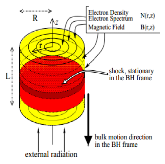
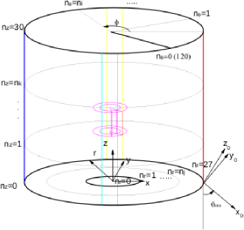
Figure 1: Left: Sketch of the geometry used in the MCFP code, adapted from Chen et al. (2012). Right: Sketch of the geometry (in the co-moving frame) of 3DPol with an enlarged illustration of one zone (in red) in the emission region. The model uses cylindrical coordinates, ($r$, $\phi$, $z$), with $n_{r}$, $n_{\phi}$, $n_{z}$ being the number of zones in the respective directions. We define a corresponding Cartesian coordinate system ($x,y,z$) where $z$ is along the jet axis and the $x$-axis is along the projection of the LOS onto the plane perpendicular to $z$. The Cartesian coordinates ($x_{0},y_{0},z_{0}$) are defined so that $x_{0}$ is along the LOS and $z_{0}$ is the projection of the jet axis onto the plane of the sky. Both Cartesian coordinate systems are in the co-moving frame of the emission region. $\theta_{\rm obs}$ is the observing angle between $x_{0}$ and $z$. Consequently, if $\theta_{\rm obs}=90^{\circ}$, ($x,y,z$) = ($x_{0},y_{0},z_{0}$). The region between the two cyan lines is the zone near the boundary of the emission region in the $-y$ direction, while the yellow region is offset from the center of the jet in the $+y$ direction. The red and blue lines represent the $x=+r_{max}$ (pre-peak) and $x=-r_{max}$ (post-peak) boundaries of the cylindrical emission region, respectively. Magenta region represents a near-central zone in the emission blob.

2.2 3D Multi-zone Synchrotron Polarization (3DPol) Code

We employ a similar geometry setup in the 3D multi-zone synchrotron polarization code. As a full 3D description is necessary to evaluate the polarization, we further divide the emission region evenly in the $\phi$ direction (Fig. 1). The assumption of axisymmetry of all parameters is still kept. As in the MCFP code, all calculations are performed in the co-moving frame of the emission region. The LOS is properly transformed via relativistic aberration. In each zone, we project the magnetic field onto the plane of sky in the comoving frame, and use the time-dependent electron distribution generated by the MCFP simulation, instead of a simple power-law, to evaluate the polarization via (Rybicki & Lightman, 1985)

$$\Pi(\omega)={P_{\perp}(\omega)-P_{\parallel}(\omega)\over P_{\perp}(\omega)+P_{\parallel}(\omega)}$$ (1)

where $\omega$ is the frequency, $P_{\parallel}(\omega)$ and $P_{\perp}(\omega)$ are the radiative powers with electric-field vectors parallel and perpendicular to the projection of the magnetic field onto the plane of the sky, respectively. $P_{\parallel}(\omega)$ and $P_{\perp}(\omega)$ are obtained via integration of the single-particle powers $P_{\parallel}(\omega,\gamma)$ and $P_{\perp}(\omega,\gamma)$ over the electron spectrum $N_{e}(\gamma)$, e.g., $P_{\parallel}(\omega)=\int_{1}^{\infty}P_{\parallel}(\omega,\gamma)\,N_{e}(\gamma)d\gamma$. Since the net electric-field vector is perpendicular to the projected magnetic field on the plane of sky in the comoving frame, the electric vector position angle, also known as polarization angle (PA), is obtained for each zone, hence we can obtain the Stokes parameters (without normalization) at every time step via

$$(I,Q,U)=L_{\nu}*(1,\Pi\cos 2\theta_{E},\Pi\sin 2\theta_{E})$$ (2)

where $L_{\nu}$ is the spectral luminosity at frequency $\nu$, $\Pi$ is the polarization percentage and $\theta_{E}$ is the electric vector position angle for that zone. The code then calculates the relative time delay to the observer for each zone, so as to take full account of the external LTTE, i.e., the time delay in the observed emission due to the spatial difference of each zone in the emission region. The internal LTTE, which is introduced through Compton scattering, is irrelevant for the present discussion of synchrotron polarization. Since the emission from different zones is incoherent, the total Stokes parameters are then calculated  by direct addition of the Stokes parameters for each zone from which emission arrives at the observer at the same time. In a post-processing routine to analyze the 3DPol output, we normalize the total Stokes parameters at every time step to evaluate the polarization, and transform the result back to the observer’s frame.

In order to test our code, we compare the total, time-dependent synchrotron spectra obtained with our 3DPol code, with the result of the MCFP code. This comparison is illustrated in Fig. 2. The overall agreement is excellent, although minor differences can be noticed, which can be attributed to the fact that the two codes use different ways to treat the radiation transfer. In particular, the larger number of zones in the 3D geometry used within 3DPol leads to slightly different LTTE compared to those in the 2D geometry of the MCFP code.

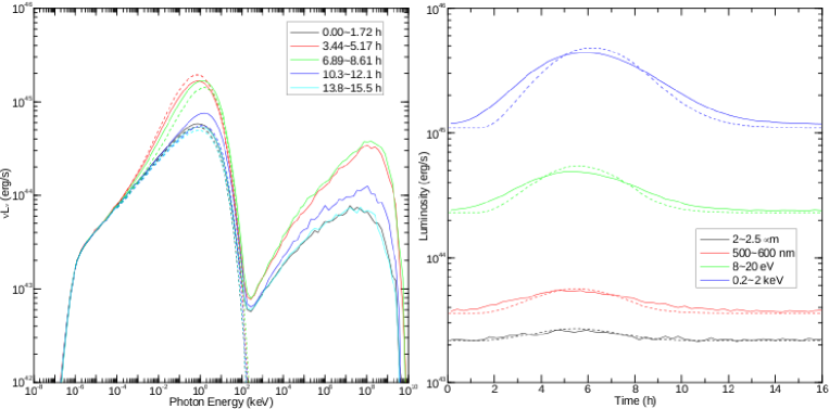
Figure 2: Comparison between the MCFP (solid lines) and the 3DPol (dashed lines) codes. Left: The SEDs of Mkn 421 for scenario 4. The time bins are chosen the same for both codes. Right: The light curves of Mkn 421 for scenario 4. The energy bins are identical as well.

3 Results

In this section, we present case studies for two blazars as examples to apply our polarization code: The high-frequency-peaked BL Lac object (HBL) Mkn 421, which is successfully fitted with a pure SSC (Synchrotron-self-Compton) model (Chen et al., 2011), and the Flat-Spectrum Radio Quasar (FSRQ) PKS 1510-089, which requires an additional EC (external Compton) component to model the $\gamma$-ray emission. In the model fit obtained in Chen et al. (2012), the external photons come from a dusty torus. Chen et al. (2011, 2012) presented model fits to the SEDs and light curves of these two blazars, using their shock-in-jet model as described above. In our polarization variability study, we will use similar parameters as in Chen et al. (2011, 2012) and compare the polarization signatures from all potential flaring scenarios 1 - 4, as described above. In order to facilitate a direct comparison, we choose the same initial parameters for all scenarios. The parameters are chosen in a way that they produce adequate flares for both sources in order to allow for direct comparisons and to mimic the observational data. Since both MCFP and 3DPol codes are time dependent, in the beginning there is a period for the electrons and the photons to reach equilibrium, before we introduce the parameter disturbance produced by the shock. The light curves shown in all our plots start after this equilibrium has been reached. As the flaring activity in the four scenarios exhibits different characteristics in duration and in strength, we define similar phases in the flare development for the purpose of a direct comparison. These phases correspond approximately to the early flare, flare peak, and late flare, and post-flare (end) states. As in Chen et al. (2011, 2012), the ratio between the emission-region dimensions $z$ and $r$ is chosen to be $\frac{4}{3}$, to mimic a spherical volume.

Due to the relativistic aberration, even though we are observing blazars nearly along the jet in the observer’s frame (typically, $\theta^{\ast}_{\rm obs}\sim 1/\Gamma$, where $\Gamma$ is the bulk Lorentz factor of the outflow along the jet), the angle $\theta_{\rm obs}$ between LOS and the jet axis in the comoving frame it is likely much larger. Specifically, if $\theta^{\ast}_{\rm obs}=1/\Gamma$, then $\theta_{\rm obs}=\pi/2$. Hence, for our base parameter studies, we set $\theta_{obs}=90^{\circ}$. This choice turns out to have a considerable effect on the result, which will be discussed in §4.1.

We define the PA in our simulations as follows. $PA=0^{\circ}$ corresponds to the electric-field vector being parallel to the projection of the jet on the plane of sky. Increasing PA corresponds to counter-clockwise rotation with respect to the LOS, to $180^{\circ}$ when it is anti-parallel to the projected jet (which is equivalent to $0^{\circ}$ due to the $180^{\circ}$ ambiguity). In all runs the zone numbers in three directions are set to $n_{z}=30$, $n_{r}=27$ and $n_{\phi}=120$, which we find to provide appropriate resolution. As is mentioned in §1, we will only focus on a parameter study and compare the general flux and polarization features of each scenario. All results are shown in the observer’s frame. Table 1 lists some key parameters.

Parameters	Initial Condition
Source	Mkn 421	PKS 1510-089
Bulk Lorentz factor $\Gamma$	$33.0$	$15.0$
$Z$ $(10^{16}cm)$	$1.0$	$8.0$
$R$ $(10^{16}cm)$	$0.75$	$6.0$
Size of the shock region in $z$ $(10^{16}cm)$	$0.1$	$0.8$
Magnetic field $B$ $(G)$	$0.13$	$0.2$
Magnetic field orientation $\theta_{B}$	$45^{\circ}$	$45^{\circ}$
Electron density $n_{e}$ $(10^{2}cm^{-3})$	$0.8$	$7.37$
Electron minimum energy $\gamma_{min}$	$10^{2}$	$50$
Electron maximum energy $\gamma_{max}$	$10^{5}$	$2*10^{4}$
Electron spectral index $p$	$2.3$	$3.2$
Electron acceleration time-scale $t_{acc}$ $(Z/c)$	$1.0$	$0.09$
Electron escape time-scale $t_{esc}$ $(Z/c)$	$0.3$	$0.015$
Orientation of LOS $\theta_{obs}$	$90^{\circ}$	$90^{\circ}$

Parameters	Scenario 1	Scenario 2
$B^{s}/B$	$\sqrt{50}$	$\sqrt{50}$
$\theta_{obs}^{s}$	$84.261^{\circ}$	$45^{\circ}$
Parameters	Scenario 3
Source	Mkn 421	PKS 1510-089
$t_{acc}^{s}/t_{acc}$	$1/5$	$1/3$

Parameters	Scenario 4
Source	Mkn 421	PKS 1510-089
Inj. $\gamma_{min}$	$10^{2}$	$3*10^{2}$
Inj. $\gamma_{max}$	$3*10^{4}$	$2*10^{5}$
Inj. $p$	$1.0$	$3.2$
Inj. rate $(erg/s)$	$5.0*10^{40}$	$5.0*10^{44}$

Table 1: Summary of model parameters. Top: Initial parameters. Notice that $\gamma_{min}$, $\gamma_{max}$ and $p$ can change before the electrons reach pre-flare equilibrium. Bottom: Shock parameters for each scenario. $s$-superscript indicates the parameters during the shock. Scenario 1&2 choose the same shock parameters for both sources. Scenario 4 lists the parameters for the injected electrons.

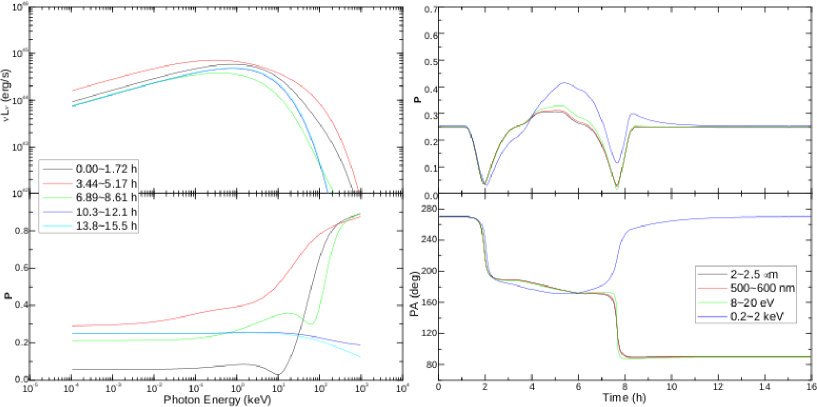
Figure 3: Flaring scenario 1 (change of direction and strength of the magnetic field) for Mkn 421. Upper left: The SEDs of Mkn 421 from the MCFP code. SEDs are chosen at approximately the beginning of the flare (black), peak (red), after peak (green), ending (blue) and back to equilibrium (cyan), with the same time bin size. Upper right: The light curves of Mkn 421 from the MCFP code, chosen at infrared (black), optical V band (red), UV (green) and soft X-ray (blue) frequencies. Lower left: The synchrotron SEDs (top) of Mkn 421 from the 3DPol code, and the polarization percentage vs. photon energy (bottom). The time bins are chosen the same as SEDs from MCFP. Lower right: The polarization percentage vs. time (top), and the polarization position angle vs. time (bottom). The energy bands are chosen the same as the light curves from MCFP.

3.1 Change of the Magnetic Field Orientation

In this scenario, the shock instantaneously increases the toroidal magnetic-field component at its location, so as to increase the total magnetic field strength and change its orientation in those zones. The new magnetic field will be kept until the shock moves out of the zone; at that time, it reverts back to its original (quiescent) strength and orientation due to dissipation.

For Mkn 421, since both synchrotron and SSC are proportional to the magnetic field strength, we see flares in both spectral bumps, though the $\gamma$-ray flare has a much lower amplitude (Fig. 3). It is also obvious that the polarization percentage has a dependence on the photon energy, although patterns above $\sim\!10$ keV are resulting from the electron distribution cut-off. In addition, it also has a time dependency. It is interesting to note that, unlike the light curve, which is symmetric in time, the polarization percentage has an asymmetric time profile, especially for higher energies. Furthermore, the polarization angles are shown to have $\sim\!180^{\circ}$ swings, although the X-ray polarization angle reverts back to its original orientation after the initial $\sim 90^{\circ}$ rotation, instead of continuing to rotate in the same direction, as in the lower-frequency bands. As we will elaborate in detail below, all these phenomena can be explained as the combined effect of electron evolution and LTTE.

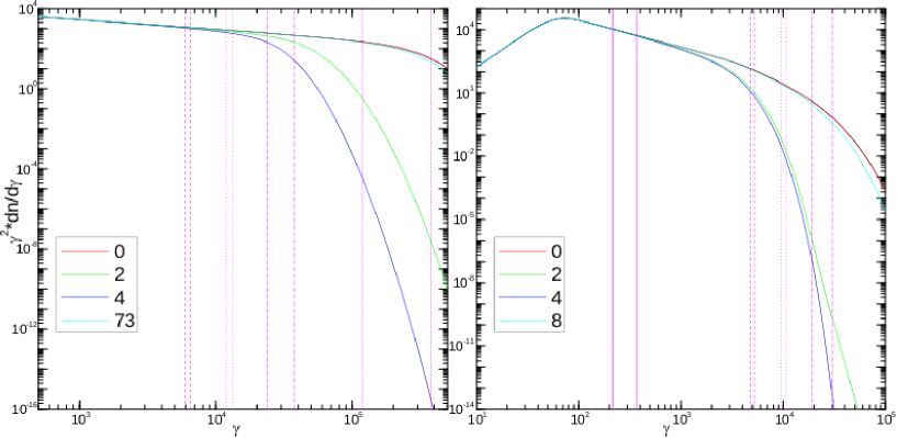
Figure 4: The electron spectra chosen at different time steps (code unit) for scenario 1 for Mkn 421 (left) and for PKS 1510-089 (right). $0$: shock turns on (identical to the pre-shock equilibrium, since the electrons have no time to evolve); $2$: in the middle of the shock; $4$: shock just turns off; and the final time step which varies by scenarios and sources is when the electron has evolved to the post-shock equilibrium (although given enough time, electrons will evolve back to the pre-shock equilibrium, but that process is extremely slow and not relevant to both luminosity and polarization). The region between magenta vertical lines represent the electron energies that correspond to the photon energies we choose in the light curves and polarization vs. time plots. Dashed is infrared, dotted is optical, dashed-dotted is UV, solid is radio (PKS 1510-089 only), short-dashed is X-rays (Mkn 421 only).

Since we assume that every zone in the jet has identical initial conditions and the shock will affect the same change everywhere, we can simply choose one zone to represent the electron evolution of the emission region (strictly speaking, due to internal LTTE and other geometric effects, different zones will be subject to slightly different SSC cooling rates; however, we have carefully checked the electron spectra and found this effect to be negligible in the cases studied here). This is illustrated in Fig. 4. When the shock reaches the zone, it will increase the magnetic field strength, hence synchrotron cooling becomes faster. Therefore the electron spectrum becomes softer while the shock is present, especially at higher electron energies, resulting in a higher possible maximal polarization percentage ($\Pi_{max}=\frac{p+1}{p+7/3}$, where $p$ is the local electron spectral index in the energy range responsible for the synchrotron emission at a given frequency, see Rybicki & Lightman (1985)). After the shock leaves the zone, the electrons gradually evolve back to equilibrium. This process takes longer at higher energies, hence the polarization percentage for more energetic photons recovers more slowly. Nevertheless, the X-ray light curve appears to evolve faster than at the lower-frequency ones. The reason for this is that the flare amplitude (compared to the equilibrium emission) is so low at X-ray frequencies, that even if the electrons have not yet reached equilibrium near the end of the flare, their contribution to the total synchrotron flux is negligible.

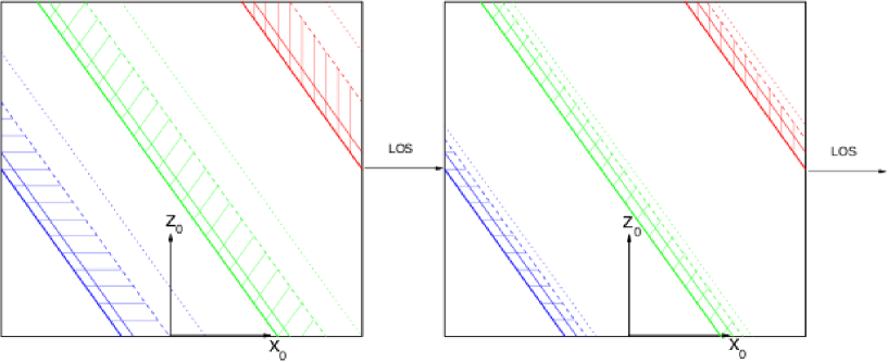
Figure 5: Sketches of a vertical slice of the cylindrical emission region at different times. Left: Sketch for Mkn 421. Right: Sketch for PKS 1510-089. The LOS is assumed to be directed in $+x$. The shock propagates through the jet from top to bottom. Solid lines demarcate regions in the jet where the shock is present at equal photon-arrival times at the observer. Red (approximately red in Fig. 1) corresponds to the pre-peak observer time, green (approximately cyan and yellow in Fig. 1) represents the flare peak and blue (approximately blue in Fig. 1) the post-peak time. The flaring region is between the bold and the thin solid lines, which correspond to the zones where the shock is currently present. The shaded region between the bold solid line and the dashed line is what we call the polarization region, containing the flaring region and the evolving region of recently shock-accelerated electrons. The dotted line represents the zones where electrons have evolved to the post-flare equilibrium. Although the electrons in the region between the dashed line and the dotted line are still evolving, their contribution to the polarization is negligible. Hence all points outside the polarization region are called the background region, or the non-flaring region.

We now discuss the influence of LTTEs on the polarization signatures. The situation is illustrated in Fig. 5. In equilibrium, the Stokes parameter $U$ will cancel out because of the axisymmetry. Additionally, despite the fact that $\theta_{B}=45^{\circ}$ implies $B_{\phi}=B_{z}$, the “effective toroidal component”, $B_{y_{0}}$, i.e., the $y_{0}$ component of $B_{\perp}$ on the plane of sky in the comoving frame, which is generally a fraction of $B_{\phi}$, is lower than the “effective poloidal component”, which is equal to $B_{z}$. Thus, the polarization is dominated by $B_{z}$. Therefore at the initial state, the polarization percentage is relatively low, and the polarization position angle is at $270^{\circ}$ (or $90^{\circ}$, considering the $180^{\circ}$ ambiguity). However, when the shock reaches the emission region, $B_{\phi}$ begins to dominate. Due to LTTE, the observer will initially only see the $+x$ side of the flaring region (Fig. 5), which has a preferential magnetic field predominantly in the $+y_{0}$ direction (Figs. 5, 6). Since the emission from the flaring region is much stronger than other parts of the emission blob, it will quickly cancel and then dominate over the polarization caused by $B_{z}$ in the background region. Hence the polarization percentage will first drop to almost zero and then rapidly increase, while the PA will drop to $\sim\!180^{\circ}$, representing an electric-field vector directed along the jet, caused by the dominant $B_{y_{0}}$. Furthermore, the electron spectrum evolves relatively slowly and the cooled high energy electrons give rise to very high $\Pi_{max}$. Therefore, the observed polarization will have contributions not only from the flaring region, but also from zones with more evolved electron distributions, where the shock has passed recently. We can observe in Fig. 5 that this “polarization region” is not symmetric from pre-peak to post-peak, resulting in an asymmetry in time, especially at higher energies.

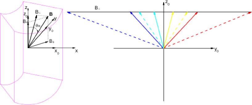
Figure 6: Sketches of magnetic field in the emission blob for $\theta_{obs}=90^{\circ}$. Left: Sketch for the magnetic field in the magenta zone shown in Fig. 1. The coordinates are illustrated in Fig. 1. The total magnetic field ${\bf B}$ in that zone is assumed to have only two components, $B_{z}$ and $B_{\phi}$; $\theta_{B}$ is the angle between ${\bf B}$ and the $z$-axis. $B_{\perp}$ is the projection of ${\bf B}$ on the plane of sky ($y_{0},z_{0}$). Right: Sketch for $B_{\perp}$ at different locations in the emission region. Red, yellow, cyan and blue correspond to the regions shown in Fig. 1. When $\theta_{obs}=90^{\circ}$, the $z_{0}$ component of $B_{\perp}$, $B_{z_{0}}=B_{z}$ throughout the emission blob, while $B_{y_{0}}\leq B_{\phi}$, and equality is obtained at the $x=+r_{max}$ (red) and $x=-r_{max}$ (blue) boundaries. The solid arrows represent the initial magnetic field orientation ($\theta_{B}=45^{\circ}$), while the dashed arrows illustrate the magnetic field orientation change in scenario 1 ($\theta_{B}\sim\!84.3^{\circ}$).

There is, however one additional factor. We can see in the light curves (Fig. 3) that the X-ray flare-to-equilibrium ratio is much smaller than at lower energies. Hence, in X-rays, the flaring region takes longer to dominate the polarization patterns, and they revert back to equilibrium faster. Furthermore, high energy electrons take longer to evolve back to equilibrium, while still providing a considerable $\Pi_{max}$. For this reason, the X-ray polarization region will be much larger than at lower energies. Therefore, when the flaring region moves to $-x$ in Fig. 5, where the preferential magnetic field is directed in $-y_{0}$, the X-ray photons will be dominated by the evolving and the background region on the $+x$ side, although lower energy photons are still dominated by the flaring region. This gives rise to the interesting phenomenon that at lower energies the PA will continuously drop to $90^{\circ}$ (which is equivalent to $270^{\circ}$ because of the $180^{\circ}$ ambiguity) as the polarization region gradually moves to $-x$ and out of the emission region; while for X-rays it instead reverts back, as the evolving region on the $+x$ side dominates the polarization, causing the magnetic field again to be preferentially oriented in the $+y_{0}$ direction, mimicking the pre-peak situation.

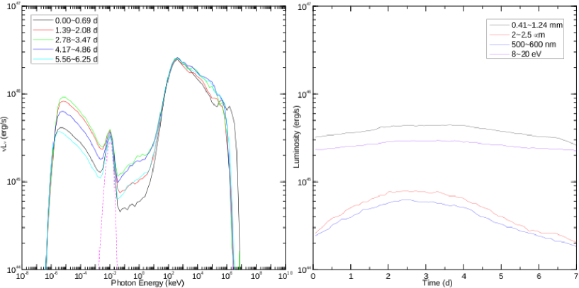
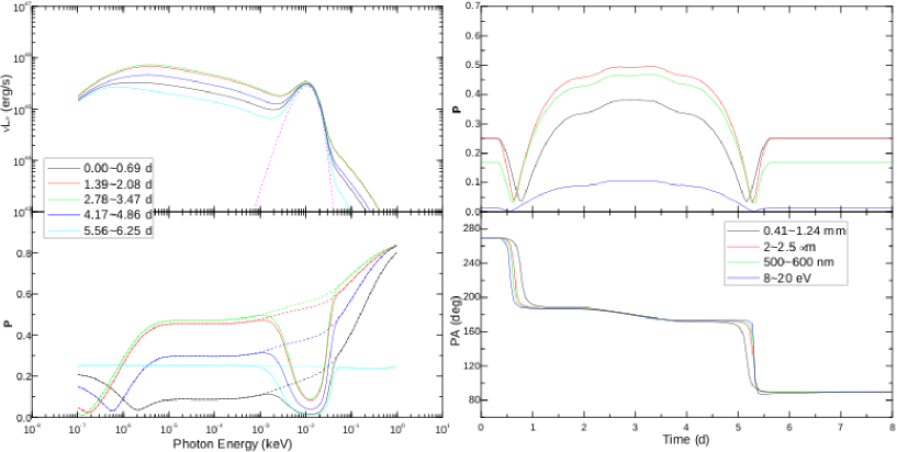
Figure 7: Flaring scenario 1 (change of direction and strength of the magnetic field) for PKS 1510-089. Upper left: SEDs of PKS 1510-089 including the external photon field contribution, at approximately the beginning of the flare (black), before peak (red), peak (green), after peak (blue) and back to equilibrium (cyan), with the dashed line for the external photon field contribution. Upper right: The light curves including the external photon field contribution, at radio (black), infrared (red), optical V band (green), UV (blue). Lower left: The synchrotron SEDs, including the external photon field, from 3DPol (top), with the dashed line for the external photon field contribution; and the polarization percentage vs. photon energy with the external photon contamination considered (bottom), where dashed lines represent the polarization percentage without the contamination. Lower right: The polarization percentage vs. time with external contamination (top), and PA vs. time (bottom).

PKS 1510-089 presents a similar situation, although there are some major differences. First, PKS1510-089 requires a dominating EC component at $\gamma$-ray energies, which is independent of the magnetic field strength. Thus in the current scenario, no flare is visible in the Compton bump (Fig. 7). Also, due to the contamination of the external thermal radiation from the dust torus, which is unpolarized, the observed polarization percentage will be considerably diminished. Furthermore, EC also introduces strong cooling to the electrons, leading to softer electron spectra (Fig. 4). As a result, $\Pi_{max}$ is much higher. Therefore at the flare peak, the polarization percentage is much higher than that in Mkn 421. Additionally, the relative electron evolution rate is faster (although the total flare time is longer than that of Mkn 421, due to the larger dimensions of the emission region). Consequently, the polarization region is much smaller, nearly equivalent to the flaring region (Fig. 5). This will make the polarization region highly symmetric from pre-peak ($+x$) to post-peak ($-x$), so that the time asymmetry found in Mkn 421 is not present in the case of PKS 1510-089. Additionally, at the flare peak the polarization region itself will concentrate on the central region (green) in Fig. 5, where $B_{y_{0}}$ is much weaker. Thus, the polarization dominated by the effective toroidal component will be diminished to a certain extent, creating a plateau at the flare peak, which is much lower than $\Pi_{max}\simeq\!0.75$. In fact, we also find a similar but weaker effect in Mkn 421, due to a larger polarization region; at X-rays, however, the very large polarization region suppresses this effect, which is why the X-ray polarization percentage exhibits a pronounced peak.

Comparing the predicted PA swings in Figs. 3 and 7 to the ones observed in several blazars, in connection with $\gamma$-ray flaring activity, one notices that the observed PA swings are more gradual than the ones predicted here. However, we remind the reader that we employ the simple assumption that the magnetic field is instantaneously changed by the shock. In reality, this change will occur over a finite amount of time. Therefore, with a more realistic time profile of the magnetic-field change, the predicted PA swing will be much smoother, instead of two rapid drops and a plateau in between. Note also that rather step-like PA rotations, similar to the features found in our simulations, have in fact been observed in S5 0716+714 by Ikejiri et al. (2011). We also point out that the $\sim\!180^{\circ}$ PA swing we show here is the result of one individual disturbance moving through the jet. If there are multiple disturbances (flares) in succession, the PA will rotate up to $180^{\circ}$ times the number of flares.

There is an ambiguity in the helical magnetic field handedness. In our model setup, we chose it to be right-handed and against the bulk motion direction. If it were left-handed, the PA rotation would appear to be in the opposite direction, but everything else would remain the same. Also notice that even the light curves will not be symmetric in time because of the asymmetry in time between the dynamics of the shock moving through the emission region and the electron cooling. However, in cases where the size of the active region, energized by the passing shock, is much smaller than the overall jet emission region (e.g., due to dominant EC cooling, the time scale for electron evolution in PKS 1510-089 is much shorter than in the case of Mkn421), this effect is minor, yielding nearly symmetric light curves.

The $\gamma$-ray emission from PKS 1510-089 is due to EC, for which changes in the synchrotron component are irrelevant, while the light curve features in our code are identical to those resulting from the MCFP code, as presented in Chen et al. (2011, 2012). In the discussion of the following scenarios, we will show the time-dependent SEDs and light curves only for Mkn 421, and restrict the discussion of PKS 1510-089 to the polarization signatures.

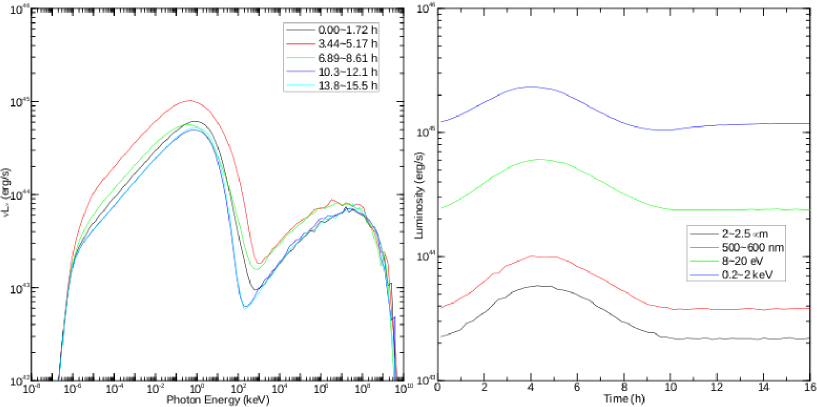
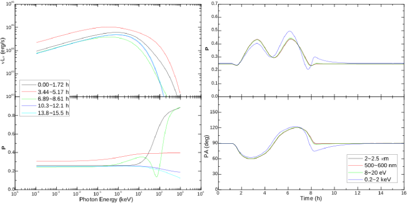
Figure 8: Flaring scenario 2 (increasing magnetic-field strength with unchanged orientation) for Mkn 421. Panels and line styles are as in Fig. 3.

3.2 Increase of the Magnetic Field Strength

In this scenario, we assume that the shock only increases the total magnetic field strength at its location, leaving its orientation unchanged. Since the electron evolution is independent of the magnetic field orientation, it appears identical to the above scenario (Fig. 4). The same applies to the SEDs and light curves. However, the polarization patterns in time show major differences. Since the magnetic field is oriented at $45^{\circ}$ to the $z$-axis, $B_{\phi}$ and $B_{z}$ will be equal throughout the emission region. Due to axisymmetry, $B_{\perp}$ in the polarization region will be confined in a cone of $\pm 45^{\circ}$. Therefore, the polarization induced by $B_{z}$, is always dominant, so that the PA will be confined to at most $(45^{\circ},135^{\circ})$. Since also the polarization of the background region is dominated by the effective poloidal component, these two will add up, resulting in a slightly higher maximal polarization percentage compared to scenario 1. However, in the immediate neighborhood of the starting and ending points of the flare, the situation is a little bit different: although the effective toroidal component $B_{y_{0}}$ is still weaker than $B_{z}$, the two components are closer in magnitude. Hence $B_{\phi}$ will diminish the polarization percentage by a small amount. Thus the two sharp dips shown in the previous polarization percentage patterns become much smaller.

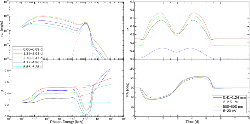
Figure 9: Flaring scenario 2 (increasing magnetic-field strength with unchanged orientation) for PKS 1510-089. Panels and line styles are as in the bottom two panels of Fig. 7.

After that, again due to LTTE, only the $+x$ side of the flaring region is observed initially, which has a preferential magnetic field oriented at $\sim\!-135^{\circ}$ (Fig. 6). Therefore the polarization is dominated by Stokes parameter $U$. Hence we observe that the polarization percentage increases and the PA moves to $45^{\circ}$. However, a basin forms at the flare peak, replacing the previous plateau, and the PA moves back to $90^{\circ}$. This is because the polarization region at the flare peak (${\it green}$ in Figs. 5, 6) is dominated by $B_{z}$, while the background region on the $-x$ and $+x$ side is just like the initial state. Therefore, the Stokes parameter $U$ contributions will cancel out due to axisymmetry, leaving the polarization dominated by $B_{z}$. The same applies when the polarization region moves to the post-peak position (blue in Fig. 5). Slight differences in the X-ray behavior are again explained by the slower electron evolution back to equilibrium.

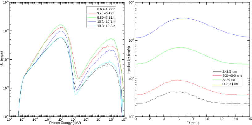
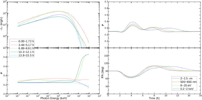
Figure 10: Scenario 3 (shortened acceleration timescale) for MKN 421. Panels and line styles are as in Fig. 3.

3.3 Shortening of the Acceleration Time Scale

In this scenario, the shock is assumed to lead to more efficient particle acceleration by instantaneously shortening the local acceleration time scale. As a result, the electrons will be accelerated to higher energy, leading to flares in both synchrotron and Compton emission (Figs. 10, 11). At the same time, the peaks of both spectral components move to considerably higher energies. However, since the magnetic field orientation remains unchanged, as in the previous scenario, the PA will stay confined to at most $(45^{\circ},135^{\circ})$.

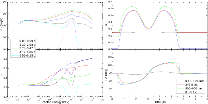
Figure 11: Scenario 3 (shortened acceleration timescale) for PKS 1510-089. Panels and line styles are as in Fig. 9.

For Mkn 421, due to the unchanged magnetic field, the higher-energy electrons take longer to cool than in the previous scenarios so that the flare duration is longer. Also, the electron spectral index remains nearly constant while the shock is present (Fig. 12), so that $\Pi_{max}$ will be nearly unchanged throughout the emission region. However, after the shock leaves a given zone, the spectrum hardens at lower energies while softening at higher energies. Since this effect acts extremely slowly and is very weak, its contribution to both luminosity and the polarization can only be seen during the post-peak phase. As a result, the polarization region dominates only because of its high luminosity. Another reason for the different polarization behavior with respect to the previous scenarios is that the polarization region is larger, containing more evolving zones. This effect is especially strong after the flare peak, when much of the emission region has been affected by the shock. Consequently, the emission region is nearly equivalent to the initial state, except that all zones radiate with higher luminosity. Therefore, we see that the polarization percentage is lower overall than in the previous scenarios, and the pre-peak polarization percentage is higher than in the post-peak phase. Just like the light curves, also the polarization percentage takes longer to evolve at higher energies.

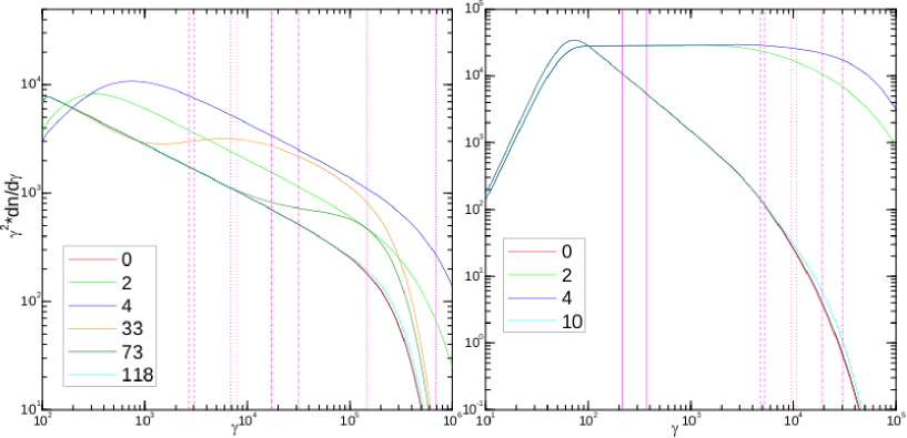
Figure 12: Time evolution of the electron spectra for scenario 3. This case has two additional lines (orange and olive) in Mkn 421 in the evolving period to show the hardening at lower energies and the softening at higher energies. Otherwise panels (left: Mkn 421; right: PKS 1510-089) and line styles are as in Fig. 4.

The situation for PKS 1510-089 is somewhat different. When the shock reaches a given zone, the shortened acceleration timescale results in a much harder spectrum, which will give lower $\Pi_{max}$. After the shock leaves the zone, due to the strong EC cooling, the electron spectrum quickly evolves back to equilibrium (Fig. 12). As a result, the polarization region is very narrow. However, a much more significant factor is that the flare-to-equilibrium luminosity ratio is very large in this case (Fig. 11). Therefore, the contribution from background regions to the polarization is negligible. Hence, although $\Pi_{max}$ is lower in the polarization region, this effect is compensated by the highly ordered magnetic field in the polarization region in the pre-peak ($\sim\!-45^{\circ}$) and post-peak ($\sim\!-135^{\circ}$) periods of the flare. The basin at the flare peak is, again, due to the axisymmetry of the polarization region. The PA shows similar features, achieving its minimum quickly at the beginning of the flare, gradually evolving to $90^{\circ}$ at the peak, then to maximum at the end of the flare and back to $90^{\circ}$ in equilibrium. There is one exception, however: At radio frequencies, the flare-to-equilibrium ratio is nearly $1$, thus we see both the polarization percentage and angle staying nearly constant.

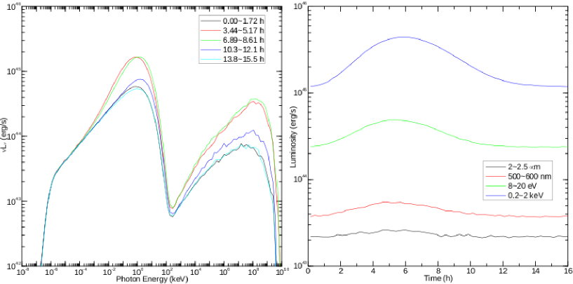
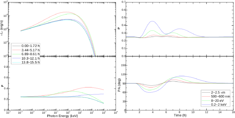
Figure 13: Scenario 4 (injection of additional high-energy electrons) for Mkn 421. Panels and line styles are as in Fig. 3.

3.4 Injection of Particles

In this scenario, the shock is assumed to continuously inject relativistic particles in the zones that it crosses (parameters for the injected electrons can be found in Table 1). The newly injected electrons will evolve and radiate immediately after the injection, in the same way as the original electrons in that zone. This scenario is similar to the previous one, except for the following differences.

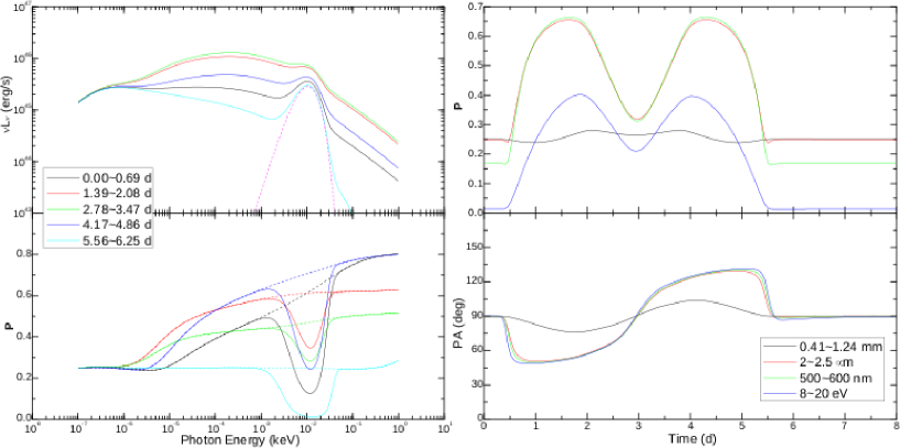
Figure 14: Scenario 4 (injection of additional high-energy electrons) for PKS 1510-089. Panels and line styles are as in Fig. 9.

First, in the case of Mkn 421, the newly injected electrons occupy an energy range not extending beyond the equilibrium electron distribution (see Fig. 15). In particular, the flare electron spectrum will not extend to higher energies than the equilibrium distribution, and therefore the electron cooling timescales remain almost unaffected. Consequently, the X-ray flare in Mkn 421 again stops earlier (Fig. 13). Second, although immediately after the injection the electron spectrum hardens, at the highest energies, it will become softer than the initial spectrum while the additional high-energy electrons cool off to lower energies, resulting in a higher $\Pi_{max}$. However, at lower energies the flare electron spectrum will generally be harder than the equilibrium spectrum. Therefore, the polarization percentage in general increases at higher energies, but decreases at lower energies (Figs. 13, 14). The same applies to PKS 1510-089, but we observe that the polarization percentage increases a little bit in radio but decreases in ultraviolet. The reason is that the radio has a little bit higher flare-to-equilibrium luminosity ratio than that in the previous scenario, while that for ultraviolet is lower, so that its polarization is contaminated more by the external photon field in the dusty torus. The PA swings follow similar patterns as in the previous scenario.

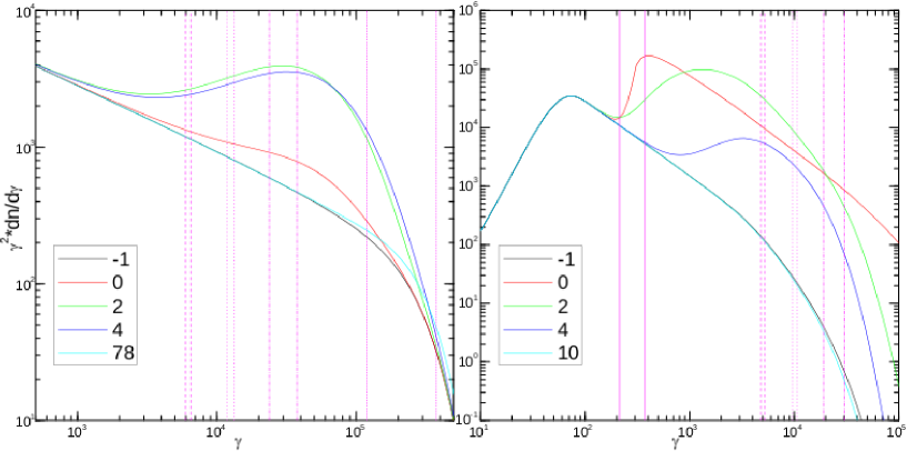
Figure 15: Time evolution of the electron spectra for scenario 4. Notice in this case the spectra at pre-shock equilibrium and at the onset of the shock are different, as the electrons are injected. Panels (left: Mkn 421; right: PKS 1510-089) and line styles are as in Fig. 4.

4 Discussion

In §3, we have shown both the energy and the time dependencies of the synchrotron fluxes and polarization patterns in a generic shock-in-jet scenario for 4 different possible mechanisms through which a shock may result in synchrotron flaring behavior. We have chosen model parameter values that have been shown to be appropriate to reproduce SEDs and light curves or Mkn 421 and PKS 1510-089. However, there are still parameter degeneracies, and some of the geometric parameters, such as the ratio between $z$ and $r$, and the viewing angle, i.e., the direction of the LOS with respect to the jet axis, $\theta_{\rm obs}$, have been fixed without strict observational constraints. In this section, we will show that the choice of these parameters may have a non-negligible influence on the predicted polarization patterns. Specifically, we use $\theta_{\rm obs}$ as an example to discuss the geometric effect on the polarization.

4.1 Dependence on the viewing angle

Throughout §3, we have assumed that we are observing the blazar jet from the side ($\theta_{\rm obs}=90^{o}$) in the co-moving frame, due to relativistic aberration. However, the relativistic beaming effects will be very similar for viewing angles that are a few degrees off this angle — in particular towards smaller viewing angles. Here we investigate the scenario 1 (for which we have shown that large PA rotations are naturally predicted) under two different viewing angles, $\theta_{\rm obs}$, namely $60^{\circ}$ and $80^{\circ}$, to illustrate this geometric effect on the polarization. $\theta_{obs}$ is unlikely to be substantially greater than $90^{\circ}$, as we are observing the blazar jet from within the relativistic beaming cone, given by $\theta^{\ast}_{\rm obs}\lesssim\!1/\Gamma$ in the observer’s frame, which corresponds to $\theta_{\rm obs}\lesssim 90^{\circ}$ in the comoving frame.

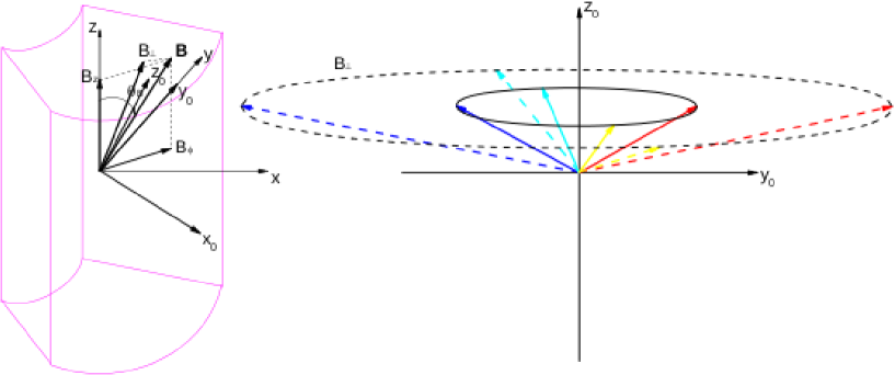
Figure 16: Similar to Fig. 6 but for $\theta_{obs}=60^{\circ}$. Here the yellow ($+y$) and cyan ($-y$) regions are not symmetric, hence the strengths of $B_{x_{0}}$ and $B_{y_{0}}$ change accordingly.

With an off-side $\theta_{\rm obs}$, the polarization region will be a bit smaller and located differently. $B_{y_{0}}$ is as well not affected, but the major change here is $B_{z_{0}}$. We observe that $B_{\perp}$, as well as the effective poloidal component $B_{z_{0}}$, is stronger in $-y$ while weaker in $+y$ (Fig. 16). Thus the axisymmetry discussed in §3 is invalid. As a result, the emission from $-y$, where $B_{\perp}$ has a relatively stronger poloidal contribution, will dominate over the emission from $+y$, where $B_{\perp}$ has a dominant toroidal contribution. However, in the initial state, although $B_{z_{0}}$ is stronger near the $-y$ axis, it is much weaker near the $+y$ axis and near the $x=\pm r_{max}$ boundaries, thus the polarization due to $B_{z_{0}}$ is overall weaker than that in the $\theta_{\rm obs}=90^{\circ}$ case. Therefore, at the pre-flare and post-flare equilibrium states, the PA has the same value as before, while the polarization percentage is lower.

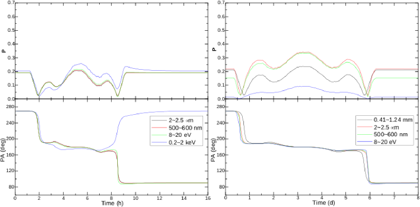
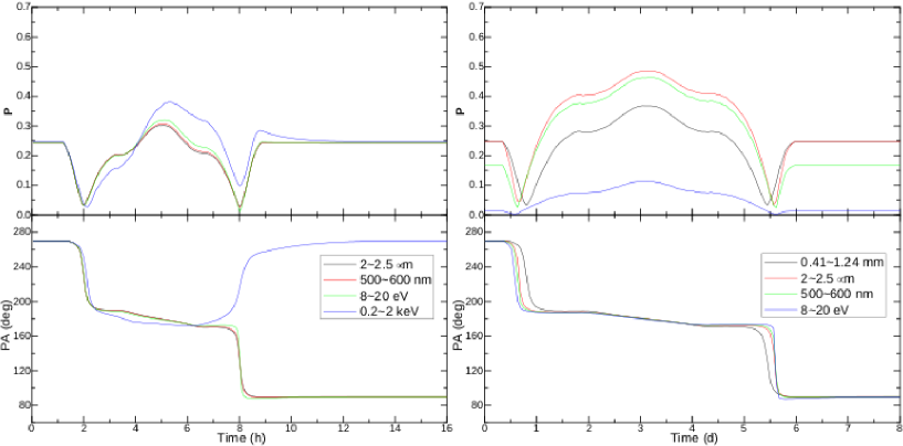
Figure 17: Polarization vs time plots for flaring scenario 1, for different viewing angles, for comparison with Figs. 3 and 7. Left column: Mkn 421. Right column: PKS 1510-089. Top row: $\theta_{obs}=60^{\circ}$. Bottom row: $\theta_{obs}=80^{\circ}$.

During the flare, however, unlike in §3.1 where amplification of $B_{\phi}$ leads to a dramatic increase in $B_{y_{0}}$, this time it also contributes to $B_{z_{0}}$, especially at the flare peak (Fig. 16). As a result, the polarization due to $B_{y_{0}}$ will be balanced out more by that from $B_{z_{0}}$. Hence the polarization caused by the toroidal magnetic-field component takes longer to reach maximum after its dominance over the original polarization due to $B_{z_{0}}$, so that the dip in the polarization percentage vs time is wider (Fig. 17), and the polarization percentage is generally lower with smaller $\theta_{obs}$ (obviously, the net polarization goes to zero in the limit $\theta_{\rm obs}\to 0^{\circ}$). This effect is particularly strong in the $\theta_{obs}=60^{\circ}$ case shown in Fig. 17, where we observe that in the pre-peak and the post-peak flaring state, there are two small dips in the polarization percentage with corresponding fluctuations in the PA. This is because the toroidal component is less dominant: At the beginning of the flare, the polarization region is small, but the toroidal component is highly ordered and is oriented in the $y_{0}$ direction (Fig. 16). This will give strong polarization in $PA=180^{\circ}$, which will quickly cancel out the background $PA=270^{\circ}$ polarization and dominate. However, when the polarization region moves closer to the center, $B_{z_{0}}$ will increase on the $-y$ side, which dominates the emission; meanwhile, the background region will be dominated by emission from the central and $-x$ regions, which will have stronger poloidal polarization than produced in the $+x$ region in the initial state. Hence, the poloidal contribution to the polarization increases. When the polarization region moves to the flare-peak position, however, the central region is affected by the shock. Although $B_{z_{0}}$ will become even stronger near the $-y$ axis, $B_{\perp}$ in its neighborhood has a stronger $B_{y_{0}}$ component. Since the polarization region extends to neighboring regions, the polarization due to $B_{y_{0}}$ will regain its dominance. The post-peak and the post-flare equilibrium evolve in the same way, as the polarization region is symmetric in the time domain, except for slight differences in X-ray.

5 Summary and Conclusions

In this paper, we have presented a detailed analysis of time- and energy-dependent synchrotron polarization signatures in a shock-in-jet model for $\gamma$-ray blazars. Our calculations employ a full 3D radiation transfer code, assuming a helical magnetic field throughout the jet, carefully taking into account light-travel-time and all other relevant geometric effects. We considered several possible mechanisms through which a relativistic shock propagating through the jet may affect the jet plasma to produce a synchrotron and high-energy flare. Among the scenarios investigated, we found that a compression of the magnetic field, increasing the toroidal field component and thereby changing the direction of the magnetic field in the region affected by the shock, leads to correlated synchrotron + SSC flaring, associated with substantial variability in the synchrotron polarization percentage and position angle. Most importantly, this scenario naturally explains large PA rotations by $\gtrsim 180^{o}$, as observed in connection with $\gamma$-ray flares in several blazars. In particular, we have falsified the claim (e.g., Abdo et al., 2010) that pattern propagation through an axisymmetric, straight jet can not produce large PA swings and rotations.

Alternative models to explain polarization variability and PA rotations, include a helical guiding magnetic field, which forces plasmoids to move along helical paths (Villata & Raiteri, 1999), and the TEMZ model by Marscher (2014). Abdo et al. (2010) have suggested that PA swings correlated with $\gamma$-ray flaring activity may result when a shock or other disturbance propagates along a curved (helical) jet. In the course of the propagation along a curved trajectory, the observer’s viewing angle with respect to the co-moving magnetic field in the active region changes, leading to possible PA swings. While such an explanation seems plausible on geometric grounds, no quantitative analysis of the resulting, correlated synchrotron and high-energy flux and polarization features has been presented for such a model, and there is currently no evidence (e.g., from observations or from MHD simulations) that blazar jets are guided by sufficiently strong, helical magnetic fields that would be able to guide relativistic pattern propagation along helical trajectories. Our analysis in this paper has demonstrated that light-travel time effects lead to much more complicated time-dependent polarization features than predicted by purely geometric considerations that neglect LTTEs.

By the stochastic nature of the TEMZ model (Marscher, 2014), it predicts generally asymmetrical light curves and random polarization patterns that do only occasionally (by coincidence) lead to large-angle PA swings, which will generally not be correlated with pronounced flaring activity at higher energies. Observed polarization angle changes do, in fact, often appear stochastic in nature, and even the polarization-swing event reported in Abdo et al. (2010) showed signs of non-unidirectional PA changes and may therefore be interpreted by a stochastic model such as the TEMZ model. The TEMZ code of Marscher (2014) takes into account SSC scattering (and its influence on electron cooling) only with seed photons from the central mach disk. Therefore, it is well applicable for blazars in which $\gamma$-ray emission and electron cooling are dominated by Comptonization of external radiation fields, which appears to be the case in low-frequency peaked blazars (FSRQs, LBLs), but not for HBLs like Mrk 421, in which the $\gamma$-ray emission is well modeled as being dominated by SSC radiation.

The strength of the PA rotation model presented here is that it very naturally explains large PA rotations, correlated with $\gamma$-ray flaring events, without the need for non-axisymmetric jet features. It is supported by observations of large-angle, uni-directional polarization swings, e.g., in 3C279 (Kiehlmann et al., 2013), which suggest that such features are unlikely to be caused by a stochastic process, but are likely the result of preferentially ordered structures. For these reasons, we prefer our quite natural explanation of PA swings correlated with synchrotron and high-energy flares, resulting from light-travel-time effects in a shock-in-jet model in a straight, axisymmetric jet embedded in a helical magnetic field.

References

- Abdo et al. (2010) Abdo, A. A., et al., 2010, Nature, 463, 919
- Aharonian et al. (2007) Aharonian, F. A., et al., 2007, ApJ, 664, L71
- Albert et al. (2007) Albert, J., et al., 2007, ApJ, 669, 862
- Böttcher (2007) Böttcher, M., 2007, ApSS, 309, 95
- Böttcher & Reimer (2012) Böttcher, M., & Reimer, A., in “Relativistic Jets from Active Galactic Nuclei”, Eds. Böttcher, M., Harris, D., & Krawczynski, H., Wiley-VCH, Berlin, 2012, Chapter 3, p. 39
- Chen et al. (2011) Chen, X., Fossati, G., Liang, E., & Böttcher, M., 2011, MNRAS, 416, 2368
- Chen et al. (2012) Chen, X., Fossati, G. Böttcher, M., & Liang, E., 2012, MNRAS, 424, 789
- D’Arcangelo et al. (2007) D’Arcangelo, F. D., et al., 2007, ApJ, 659, L107
- Ikejiri et al. (2011) Ikejiri, Y., et al., 2011, PASJ, 63, 639
- Kiehlmann et al. (2013) Kiehlmann, S., et al., 2013, arXiv:1311.3126
- Krawczynski et al. (2012) Krawczynski, H., Böttcher, M., & Reimer, A., in “Relativistic Jets from Active Galactic Nuclei”, Eds. Böttcher, M., Harris, D., & Krawczynski, H., Wiley-VCH, Berlin, 2012, Chapter 8, p. 215
- Laing (1980) Laing, R., 1980, MNRAS, 193, 439
- Lyutikov et al. (2005) Lyutikov, M., Pariev, V. I., & Gabuzda, D. C., 2005, MNRAS, 360, 869
- Marscher et al. (2008) Marscher, A. P., et al., 2008, Nature, 452, 966
- Marscher et al. (2010) Marscher, A. P., et al., 2010, ApJ, 710, L126
- Marscher (2014) Marscher, A. P., 2014, ApJ, 780, 87
- Pushkarev et al. (2005) Pushkarev, A. B., Gabuzda, D. C., Vetukhnovskaya, Yu. N., & Yakimov, V. E., 2005, MNRAS, 356, 859
- Rybicki & Lightman (1985) Rybicki, G. B., Lightman, A. P. 1985, Radiative processes in Astrophysics, Wiley-VCH
- Villata & Raiteri (1999) Villata, M., & Raiteri, C. M., 1999, A&A, 347, 30
- Westfold (1959) Westfold, K. C., 1959, ApJ, 130, 241
- Zhang & Böttcher (2013) Zhang, H., & Böttcher, M., 2013, ApJ, 774, 18