Current-driven filamentation upstream of magnetized relativistic collisionless shocks

Abstract

The physics of instabilities in the precursor of relativistic collisionless shocks is of broad importance in high energy astrophysics, because these instabilities build up the shock, control the particle acceleration process and generate the magnetic fields in which the accelerated particles radiate. Two crucial parameters control the micro-physics of these shocks: the magnetization of the ambient medium and the Lorentz factor of the shock front; as of today, much of this parameter space remains to be explored. In the present paper, we report on a new instability upstream of electron-positron relativistic shocks and we argue that this instability shapes the micro-physics at moderate magnetization levels and/or large Lorentz factors. This instability is seeded by the electric current carried by the accelerated particles in the shock precursor as they gyrate around the background magnetic field. The compensation current induced in the background plasma leads to an unstable configuration, with the appearance of charge neutral filaments carrying a current of the same polarity, oriented along the perpendicular current. This “current-driven filamentation” instability grows faster than any other instability studied so far upstream of relativistic shocks, with a growth rate comparable to the plasma frequency. Furthermore, the compensation of the current is associated with a slow-down of the ambient plasma as it penetrates the shock precursor (as viewed in the shock rest frame). This slow-down of the plasma implies that the “current driven filamentation” instability can grow for any value of the shock Lorentz factor, provided the magnetization $\sigma\,\lesssim\,10^{-2}$. We argue that this instability explains the results of recent particle-in-cell simulations in the mildly magnetized regime.

1 Introduction

The physics of particle acceleration at relativistic collisionless shock waves plays a key role in the description of a number of powerful astrophysical objects, e.g. blazars, pulsar wind nebulae, gamma-ray bursts etc. One of the lessons learned in the past decade in this field of research, is the importance of the non-linear relationship that ties the acceleration process and the generation of micro-turbulence in the shock vicinity. It was anticipated early on that the self-generation of micro-turbulence on length scales much smaller than the gyroradius of the accelerated particles is a necessary condition for the proper development of the relativistic Fermi process (Lemoine et al. 2006), in agreement with test particle Monte Carlo simulations (Niemiec et al. 2006). This small-scale nature of the turbulence comes with a number of important consequences, most notably the limited maximal energy of particles accelerated at ultra-relativistic shock waves, e.g. Kirk & Reville (2010), Bykov et al. (2012), Plotnikov et al. (2013a).

The particle-in-cell (PIC) numerical simulations of Spitkovsky (2008a,b) have confirmed the validity of these arguments and offered a more exhaustive picture of the acceleration process in the ultra-relativistic unmagnetized limit. These simulations have shown that the accelerated (supra-thermal) particle population excites filamentation instabilities upstream of unmagnetized shock waves (meaning, shock waves propagating in an unmagnetized medium), see also Nishikawa et al. (2009); these instabilities build up a magnetic barrier on plasma scales $c/\omega_{\rm p}$ and at the same time serve as scattering centers for the acceleration process. As the magnetic field energy density grows to an equipartition fraction $\epsilon_{B}\,\sim\,10^{-1}$ ($\epsilon_{B}$ denotes the fraction of incoming kinetic energy flux in the shock front rest frame stored in magnetic energy), incoming particles can be isotropized on a coherence length scale of the order of $\sim 10c/\omega_{\rm p}$, thereby initiating the shock transition. The gyroradius of accelerated particles remains larger than this length scale and the Fermi acceleration process develops as anticipated. These simulations have been confirmed, and followed by further PIC simulations with different conditions, in particular regarding the degree of magnetization of the upstream (background) plasma, the obliquity of the magnetic field and the nature (pairs vs electron-proton) of the incoming flow (e.g. Keshet et al. 2009, Martins et al. 2009, Sironi & Spitkovsky 2009, 2011, Haugbølle 2011, Sironi et al. 2013).

The physics of the electromagnetic instabilities that lead to the formation of a ultra-relativistic collisionless shock and to the self-sustainance of the shock have naturally received a lot of attention: e.g. Hoshino & Arons (1991), Hoshino et al. (1992) and Gallant et al. (1992) for magnetized shock waves; for weakly magnetized shock waves, see e.g. Medvedev & Loeb (1999), Wiersma & Achterberg (2004), Lyubarsky & Eichler (2006), Milosavljević & Nakar (2006), Achterberg & Wiersma (2007), Achterberg et al. (2007), Pelletier et al. (2009), Lemoine & Pelletier (2010, 2011), Bret et al. (2010), Rabinak et al. (2011) and Shaisultanov et al. (2012). To summarize in a few lines the current understanding, the Weibel/filamentation instability appears to play a leading role in the generation of the small-scale magnetic field in the weakly magnetized shock limit, although electrostatic oblique modes and Buneman modes retain their importance in pre-heating the electrons away from the shock front; see the discussion in Lemoine & Pelletier (2011). At strongly magnetized shock waves, the synchrotron maser instability is recognized as the leading agent of dissipation, e.g. Hoshino & Arons (1991), Hoshino et al. (1992) and Gallant et al. (1992).

However, at intermediate magnetizations and/or very large Lorentz factors, the physics remains poorly known. Indeed, the filamentation instability and other two stream modes cannot be excited in these regions of parameter space, because the timescale on which the incoming particles cross the precursor becomes shorter than the timescale on which such instabilities can be excited (Lemoine & Pelletier 2010, 2011). Therefore, how the shock is structured in such conditions remains an open question.

We report here on a new current-driven instability which is likely to emerge as the dominant instability in this range of magnetization and at very large Lorentz factors. The electric current is carried by the suprathermal particles (or shock reflected particles) and results from their gyration in the background magnetic field: assuming that the magnetic field is oriented along the $\boldsymbol{z}$ axis, while the incoming plasma flows along $\boldsymbol{-x}$ in the shock rest frame, the current is generated along $\boldsymbol{-y}$, since the Lorentz force deflects positive and negative suprathermal particles in opposite directions. As the ambient plasma penetrates the precursor, it develops a compensating current along $\boldsymbol{+y}$. This configuration is found to be unstable, because a current fluctuation can couple to a density fluctuation and excite a combination of extraordinary modes and compressive modes of the ambient plasma. This will be made explicit further on.

As viewed from the rest frame of the ambient plasma, this perpendicular electric current is extraordinarily large. If one writes $\xi_{\rm cr}$ the fraction of incoming kinetic energy flux carried by the suprathermal particles – see Eq. (1) below – with $\xi_{\rm cr}\sim 0.1$ indicated by PIC simulations, $\gamma_{\rm sh}\,\gg\,1$ the Lorentz factor of the shock wave in the ambient plasma frame and $n_{\rm u}$ the proper density of the ambient plasma, the induced current reads $j_{y,\rm cr}\,\sim\,\gamma_{\rm sh}\xi_{\rm cr}n_{\rm u}ec$. For $\gamma_{\rm sh}\xi_{\rm cr}\,\gtrsim\,1$, as expected in ultra-relativistic shocks, this current cannot be compensated by the ambient plasma at rest. As we will demonstrate, the latter is actually accelerated to relativistic velocities relatively to its initial rest frame and it is squashed to an apparent density $\sim\gamma_{\rm sh}\xi_{\rm cr}n_{\rm u}$ in the frame in which there is no bulk motion along $\boldsymbol{x}$ (denoted ${\cal R}$ in the following); then, particle motion at relativistic velocities along $\boldsymbol{y}$ leads to current compensation.

In this work, we focus on an electron-positron shock; in electron-ion shocks, a similar current develops but excites other modes, in particular Whistler waves. This case will be discussed in a forthcoming paper. In Section 2, we discuss the physics of the instability at the linear level, using a relativistic two-fluid model for the incoming background plasma exposed to a rigid external current set by the suprathermal particles. In Section 3, we discuss the relevance of this instability in relativistic collisionless shocks and compare it to results of recent PIC simulations. We discuss the structure of the precursor in Appendix A and provide conclusions in Sec. 4.

2 Current-driven filamentation instability

We describe the shock precursor as follows, in the shock front frame. The incoming plasma flows with 4-velocity $u_{x}<0$, carrying magnetic field $\boldsymbol{B}=B_{z}\,\boldsymbol{z}$ and convective electric field $\boldsymbol{E}=\gamma_{\rm sh}\beta_{\rm sh}B_{\rm u}\,\boldsymbol{y}$, with $\beta_{\rm sh}<0$ the velocity of the incoming background plasma in the shock rest frame in units of $c$, i.e. $\gamma_{\rm sh}\,\equiv\,\left(1-\beta_{\rm sh}^{2}\right)^{-1/2}$. In principle, $B_{z}$ depends on $x$, while $B_{\rm u}$ corresponds to the upstream magnetic field measured in the upstream rest frame well beyond the precursor. The precursor also contains a population of relativistic suprathermal particles, which rotate around $\boldsymbol{B}$ and thereby induce a current along $\boldsymbol{y}$, $\boldsymbol{j_{\rm cr}}\sim-\gamma_{\rm sh}\xi_{\rm cr}n_{\rm u}ec\,\boldsymbol{y}$. The quantity $\xi_{\rm cr}$ characterizes the fraction of the incoming particle energy carried by the suprathermal particles:

$$\xi_{\rm cr}\,\equiv\,\frac{e_{\rm cr}}{\gamma_{\rm sh}^{2}n_{\rm u}mc^{2}}\ ,$$ (1)

with $e_{\rm cr}\,=\,n_{\rm cr}\gamma_{\rm sh}mc^{2}$ in the shock frame, assuming that the supra-thermal particles carry a density $n_{\rm cr}$ and typical Lorentz factor $\gamma_{\rm sh}$; from Eq. (1), one derives $n_{\rm cr}\,=\,\gamma_{\rm sh}\xi_{\rm cr}n_{\rm u}$, whence the expression for the current density $\boldsymbol{j_{\rm cr}}$.

The spatial profile of this current and the overall structure of the precursor are described in detail in App. A; Fig. 1 offers a sketch of the precursor. The typical size of the precursor is $c/\omega_{\rm c}$, with $\omega_{\rm c}=eB_{\rm u}/(mc)$ the upstream cyclotron frequency; this size also corresponds to the typical gyration radius $r_{\rm L}$ of the suprathermal particles in the shock front rest frame, whose typical Lorentz factor $\sim\gamma_{\rm sh}$.

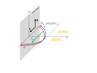
Figure 1: Sketch of the precursor of a relativistic magnetized pair shock, as viewed in the shock front rest frame. The reflected/shock-accelerated suprathermal particles (in red and blue) gyrate in the background magnetic field and accelerate parallel to the convective electric field, thereby generating a net perpendicular current $j_{y,\rm cr}$. The incoming plasma must compensate this current as it penetrates the precursor.

As the incoming particles cross the precursor, they are deflected along $\boldsymbol{y}$ in order to compensate the cosmic ray perpendicular current. Positrons drift towards $\boldsymbol{+y}$ while electrons drift towards $\boldsymbol{-y}$. The absolute value of the 4-velocity $y-$component for both fluids is equal, $|u_{y}|\sim\gamma_{\rm sh}\xi_{\rm cr}$ (in units of c), hence $|u_{y}|\,\gtrsim\,1$ is expected for relativistic shocks, possibly $|u_{y}|\,\gg\,1$.

The deflection of the incoming flow along $\boldsymbol{y}$ implies a substantial deceleration of the flow along $\boldsymbol{x}$, which has drastic consequences regarding the development of the instability. The profile of the velocity of the flow is discussed in detail in App. A, but one can apprehend this slow-down as follows: the total Lorentz factor of the flow remains large, in particular the total 3-velocity $|\boldsymbol{\beta}|\sim 1$, up to corrections of order $\gamma_{\rm sh}^{-2}$; however, a transverse velocity develops with magnitude $|\beta_{y}|\,\simeq\,\xi_{\rm cr}$; the combination of these two facts implies that $\beta_{\rm x}$ deviates from unity by quantities of order $\gamma_{\rm sh}^{-2}$ or $\xi_{\rm cr}^{2}$, whichever is larger. In other words, assuming that $\gamma_{\rm sh}\xi_{\rm cr}\,\gg\,1$, as expected in ultra-relativistic shocks, leads to $|\beta_{\rm x}|\,\simeq\,1-\xi_{\rm cr}^{2}/2$. If $\gamma_{\rm sh}\xi_{\rm cr}\,\ll\,1$, $\beta_{\rm x}$ remains unchanged compared to the asymptotic value outside the precursor.

This is a quite remarkable feature: the compensation of the current slows down the incoming plasma down to the (longitudinal) velocity $\beta_{\rm x}$; thus, the ${\cal R}$ frame which corresponds to the instantaneous rest frame of the plasma, in which there is no bulk motion along $\boldsymbol{x}$, moves with velocity $\beta_{{\cal R}|\rm sh}=\beta_{\rm x}$ relative to the shock front rest frame. At large values of the current, $\gamma_{\rm sh}\xi_{\rm cr}\,\gg\,1$, the relative Lorentz factor between the ${\cal R}$ frame and the shock front rest frame becomes of the order of $1/\xi_{\rm cr}$, independent of the far upstream Lorentz factor. In this sense, the shock precursor plays the role of a buffer, with important consequences for the physics of the shock, discussed in Sec. 3.

The Lorentz factor that corresponds to the relative velocity between this new rest frame ${\cal R}$ and the far upstream rest frame is easily calculated and well approximated by:

$$\gamma_{{\cal R}|\rm u}\,\simeq\,{\rm max}\left(1,\gamma_{\rm sh}\xi_{\rm cr}/2\right)\ .$$ (2)

In the following, we analyze the evolution of the instability in the linear regime by adopting a relativistic two-fluid description of the incoming plasma, where two-fluid refers to the electron and positron components of the background plasma. This means, in particular, that we neglect the response of the cosmic rays and we treat as external the current that these suprathermal particles carry. The latter assumption is discussed in Sec. 3. In this section, we assume that current compensation is achieved to high accuracy in the shock precursor, as motivated by our discussion in Sec. A.1; see also the discussion in Sec. 5.3.1 of Lemoine & Pelletier (2011). This two-fluid description allows us to probe the physics of the instability up to the inertial scale of the incoming plasma, where the growth rate is found to peak.

We write and solve the system in the instantaneous rest frame ${\cal R}$ of the plasma, in which there is no bulk motion along $\boldsymbol{x}$. In such a rest frame, the instability is expected to be absolute (vs convective), provided the growth rate exceeds the inverse crossing time of the precursor. In the ${\cal R}$ frame, $u_{x|{\cal R}}\,=\,0$ (henceforth, all quantities concern the incoming plasma), but the (unperturbed) background electric and magnetic fields read

$$B_{z|{\cal R}}\,=\,\gamma_{{\cal R}|\rm u}B_{\rm u},\quad E_{y|{\cal R}}\,=\,-\gamma_{{\cal R}|\rm u}\beta_{{\cal R}|\rm u}B_{\rm u}\ .$$ (3)

2.1 Linear analysis

For simplicity, we assume the plasma and the velocity profile to be uniform throughout the precursor. It is possible to incorporate the terms associated to the variation of the profile by writing the system first in the shock front frame, then boosting it to the instantaneous rest frame of the incoming plasma. The new terms that appear contain spatial derivatives (along $x$) of the various unperturbed quantities. The typical magnitude of these inhomegeneous terms relative to the other terms is of order $\omega_{\rm c}/\omega$ in Fourier variables; therefore, the above assumption will be justified provided $|k_{x}|\,\gg\,\omega_{\rm c}/c$. As we show in the following, the growth rate peaks at values close to $\omega_{\rm p}$ on short wavelengths, i.e. $k\,\simeq\,\omega_{\rm p}/c$; this therefore justifies the above approximation of a uniform precursor.

Our linear analysis is based on a relativistic two-fluid model of the background plasma subject to the external current imposed by the gyrating supra-thermal particles. We thus perturb all variables of the incoming flow and the electromagnetic structure. The unperturbed equations are:

$$\partial_{\mu}\left(n_{\pm}u_{\pm}^{\mu}\right) \,=\, 0$$

$$\partial_{\mu}T^{\mu\nu}_{\pm} \,=\, \pm en_{\pm}u_{\pm}^{\mu}\,F^{\nu}_{\,\,\mu}\ .$$ (4)

The indices $\pm$ refer to the positron/electron species of the background plasma, $u^{\mu}_{\pm}$ to the $4-$velocity and $T^{\mu\nu}_{\pm}$ to the corresponding energy-momentum tensors. The perturbed system then reads:

$$u^{\mu}_{\pm}\partial_{\mu}\left(\frac{\delta n_{\pm}}{n}\right)+\partial_{\mu}\delta u^{\mu}_{\pm} \,=\, 0$$

$$u_{\pm}^{\mu}\partial_{\mu}\delta u^{\nu}_{\pm}+\beta_{\rm s}^{2}\partial^{\nu}\left(\frac{\delta n_{\pm}}{n}\right) \,=\, \pm\frac{e}{m}\delta u^{\sigma}_{\pm}F^{\nu}_{\,\,\sigma}\pm\frac{e}{m}u^{\sigma}_{\pm}\delta F^{\nu}_{\,\,\sigma}\ ,$$

together with the Maxwell equations. We have implicitly assumed a cold background plasma limit, although we incorporate temperature effects through the sound velocity $\beta_{\rm s}$.

We recombine the two fluid variables $\delta n_{\pm}$ and $\delta u_{\pm}^{\mu}$ into:

$$\delta n \,\equiv\, \frac{\delta n_{+}+\delta n_{-}}{2},\quad\delta\rho\,\equiv\,\frac{\delta n_{+}-\delta n_{-}}{2}$$ (6)

$$\delta u^{\mu} \,\equiv\, \frac{\delta u_{+}^{\mu}+\delta u_{-}^{\mu}}{2},\quad\Delta u^{\mu}\,\equiv\,\frac{\delta u_{+}^{\mu}-\delta u_{-}^{\mu}}{2}\ .$$ (7)

Of course, to zeroth order, $n_{-}=n_{+}\equiv n$, $u_{-}^{0}=u_{+}^{0}\equiv u^{0}$, $u_{+,y}=-u_{-,y}\equiv u_{y}$. Furthermore, $\left(u_{\pm}^{\mu}+\delta u_{\pm}^{\mu}\right)\left(u_{\pm\mu}+\delta u_{\pm\mu}\right)=-1$ implies

$$\delta u^{0}\,=\,\beta_{y}u^{0}\Delta u_{y}\ ,\quad\Delta u^{0}\,=\,\beta_{y}u^{0}\delta u_{y}\ ,$$ (8)

with $\beta_{y}\,\equiv\,u_{y}/u^{0}$. In the ${\cal R}$ frame, in which we are working here, $u^{0}\,=\,(1+u_{y}^{2})^{1/2}$; therefore $u_{y}\,\sim\,\gamma_{\rm sh}\xi_{\rm cr}\,\gg\,1$ at large shock Lorentz factors implies $|\beta_{y}|\,\sim\,1$. In the limit $\gamma_{\rm sh}\xi_{\rm cr}\,\gg\,1$ (but $\xi_{\rm cr}\,\ll\,1$), the parameters $\gamma_{{\cal R}|\rm u}/u^{0}\,\simeq\,1/2$ and $\beta_{{\cal R}|\rm u}\,\simeq\,1$.

The perturbed current $\delta j^{\mu}=\delta j^{\mu}_{+}+\delta j^{\mu}_{-}$ reads

$$\delta j^{0} \,=\, 2nec\,\left(\Delta u^{0}+u^{0}\delta\rho/n\right),$$ (9)

$$\delta j_{x} \,=\, 2nec\,\Delta u_{x},$$ (10)

$$\delta j_{y} \,=\, 2nec\,\left(\Delta u_{y}+\beta_{y}u^{0}\delta n/n\right),$$ (11)

$$\delta j_{z} \,=\, 2nec\,\Delta u_{z}\ .$$ (12)

We define the plasma frequency following: $\omega_{p}^{2}\,=\,\omega_{p+}^{2}+\omega_{p-}^{2}\,=\,8\pi ne^{2}/m_{e}$, and the magnetization parameter:

$$\sigma\,=\,\frac{B_{\rm u}^{2}}{8\pi nm_{e}c^{2}}\,=\,\frac{\omega_{\rm c}^{2}}{\omega_{\rm p}^{2}}\ .$$ (13)

The full dispersion relation is calculated from the linear system discussed in App. B, by going through Fourier variables, then taking the determinant of the matrix using the Mathematica package. This dispersion relation is too lengthy to be reported here.

However, it can be given in the following form in the 1D approximation $k_{y}=k_{z}=0$, cold plasma limit $\beta_{\rm s}=0$:

$$\begin{split}\omega^{5}+i\beta_{{\cal R}|\rm u}\beta_{y}\kappa\omega_{\rm c}\omega^{4}\\ -\left[k_{x}^{2}c^{2}+\kappa^{2}\omega_{\rm c}^{2}+(1-\beta_{y}^{2})\omega_{\rm p}^{2}\right]\omega^{3}-i\beta_{{\cal R}|\rm u}\beta_{y}\kappa k_{x}^{2}c^{2}\omega_{\rm c}\omega^{2}\\ +\left(\kappa^{2}k_{x}^{2}c^{2}\omega_{\rm c}^{2}-\beta_{y}^{2}k_{x}^{2}c^{2}\omega_{\rm p}^{2}-i\kappa\beta_{y}^{3}k_{x}c\omega_{\rm c}\omega_{\rm p}^{2}\right)\omega\\ -i\beta_{{\cal R}|\rm u}\beta_{y}^{3}\kappa k_{x}^{2}c^{2}\omega_{\rm c}\omega_{\rm p}^{2}\,=\,0\\ \end{split}$$

We recall here the definition $\kappa\,\equiv\,\gamma_{{\cal R}|\rm u}/u^{0}$, see App. B. The growth rate is represented as a function of $k_{x}$ for various values of the parameters $\beta_{y}$ and $\sigma$ in Fig. 2. The global trend that emerges is a maximal growth rate

$$\Im\omega\,\sim\,\beta_{y}\omega_{\rm p}\quad\left(k_{x}c\,\sim\,\omega_{\rm p},\,\,\beta_{y}\,\gg\,\sqrt{\sigma},\,\,\beta_{y}\,\gg\,\beta_{\rm s}\right)\ .$$ (14)

The growth rate collapses as soon as one of the conditions indicated in the brackets is no longer satisfied. The last condition $\beta_{y}\,\gg\,\beta_{\rm s}$ is typical of current-driven instabilities: as the temperature rises and the thermal velocity exceeds the drift velocity, the instability disappears. However, we do not expect this situation in ultra-relativistic pair shocks with $\gamma_{\rm sh}\xi_{\rm cr}\,\gg\,1$, since $\beta_{y}\,\sim\,1$ in that limit, while the heating of the incoming flow inside the precursor remains limited to sub-relativistic velocities, see e.g. Lemoine & Pelletier (2011) for a discussion and Spitkovsky (2008a) for PIC simulations.

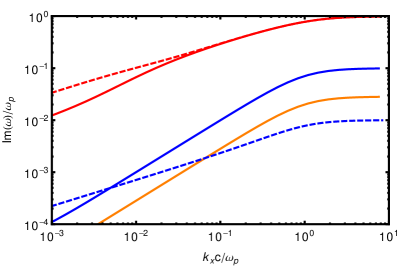
Figure 2: Growth rate $\Im\omega/\omega_{\rm p}$ vs $k_{x}c/\omega_{\rm p}$ for $k_{y}=k_{z}=0$. In solid lines, $\sigma=10^{-4}$, $\beta_{\rm s}=0$ and from top to bottom, $\beta_{y}=0.99$ (red, corresponding to $u_{y}=\gamma_{\rm sh}\xi_{\rm cr}\,\simeq\,7.0$), $\beta_{y}=0.1$ (blue, corresponding to $\gamma_{\rm sh}\xi_{\rm cr}=0.1$), and $\beta_{y}=0.03$ (orange, $\gamma_{\rm sh}\xi_{\rm cr}=0.03$). In dashed lines, same as above for $\sigma=10^{-2}$ (the growth is strongly suppressed for $\beta_{y}=0.03$ in this case).

In the 2D $k_{y}=0$, cold plasma ($\beta_{\rm s}=0$), and small current limit ($\xi_{\rm cr}\gamma_{\rm sh}\,\ll\,1$, in which case $\beta_{{\cal R}|\rm u}\,\sim\,0$ and $u^{0}\,\sim\,1$), the dispersion relation also reduces to the compact form:

$$\omega^{6}-\omega^{4}\left(\omega_{\rm p}^{2}+\omega_{\rm c}^{2}+k_{x}^{2}c^{2}+k_{z}^{2}c^{2}-\beta_{y}^{2}\omega_{\rm p}^{2}\right)$$

$$+\,\omega^{2}\left[(k_{x}^{2}+k_{z}^{2})c^{2}\omega_{\rm c}^{2}-\beta_{y}^{2}(k_{x}^{2}+k_{z}^{2})c^{2}\omega_{\rm p}^{2}-i\beta_{y}^{3}k_{x}c\omega_{\rm p}^{2}\omega_{\rm c}\right]$$

$$+\,\beta_{y}^{2}k_{z}^{2}c^{2}\omega_{\rm c}^{2}\omega_{\rm p}^{2}\,=\,0\ .$$ (15)

In this limit, the instability can be shown to result from a coupling between the high frequency branch of the extraordinary mode with the acoustic mode, as discussed in the following Sec. 2.2.

We now present numerical solutions of this dispersion relation in the various 2D planes: $(k_{x},k_{z})$ in Fig. 3 assuming $k_{y}=0$; $(k_{x},k_{y})$ in Fig. 4 assuming $k_{z}=0$; and $(k_{y},k_{z})$ in Fig. 5 assuming $k_{x}=0$.

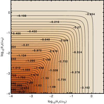
Figure 3: Contour plot of ${\rm log}_{10}\left(\Im\omega/\omega_{\rm p}\right)$ assuming $k_{y}\,=\,0$, for $\gamma_{\rm sh}u_{y}\,=\,7$ (i.e. $\beta_{y}\,=\,0.99$), $\sigma=10^{-3}$, $\beta_{\rm s}\,=\,0$.

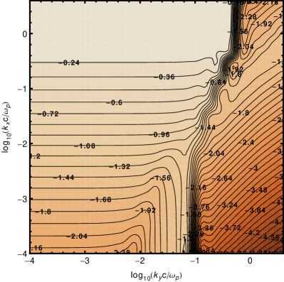
Figure 4: Same as Fig. 3, in the plane $(k_{x},k_{y})$, for $k_{z}=0$.

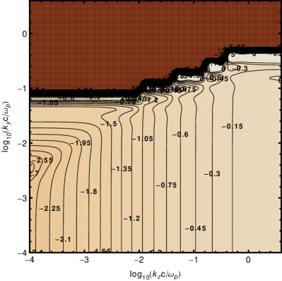
Figure 5: Same as Fig. 3, in the plane $(k_{y},k_{z})$, for $k_{x}=0$. The growth rate vanishes at large values of $k_{y}$.

The global trend that emerges from these numerical simulations is, here as well, a maximum growth rate of order $\beta_{y}\omega_{\rm p}$ at wavenumbers $\sim\omega_{\rm p}$, provided the thermal dispersion velocity $\beta_{\rm s}$ remains much smaller than the drift velocity $\beta_{y}$.

2.2 Interpretation and analytical approximations

The above instability can be best understood in the limit $k_{y}\,=\,0$, in the non-relativistic regime $\beta_{y}\,\ll\,1$, which formally corresponds to $\gamma_{\rm sh}\xi_{\rm cr}\,\ll\,1$. In this limit, one can neglect the acceleration of the plasma relative to the far upstream, $\beta_{{\cal R}|\rm u}\,\sim\,0$, so that the convective electric field can be neglected; furthermore, $\kappa=\gamma_{{\cal R}|\rm u}/u^{0}\,\sim\,1$. Although relativistic shock waves should rather lead to $\gamma_{\rm sh}\xi_{\rm cr}\,\gtrsim\,1$, we find little difference in the growth rate between the above approximation and the numerical calculation, suggesting that it remains a good approximation.

In this $\beta_{y}\,\ll\,1$ regime, the instability involves only velocity fluctuations $\delta u_{x}$, $\delta u_{z}$, a density fluctuation $\delta n$, and electromagnetic perturbations $\delta B_{x}$, $\delta B_{z}$ and $\delta E_{y}$. One then finds that a combination of the acoustic mode along $B_{z}$ and the high frequency superluminal branch of the extraordinary mode is destabilized by the drift motion that results from the compensation of the current $j_{y}$.

To see this, we use the perturbed $y-$component of the electromagnetic vector potential $\delta A_{y}$ and the displacement $\boldsymbol{\xi}$ of the plasma. Maxwell equations then imply

$$c^{2}\boldsymbol{\nabla\cdot\nabla}\,\delta A_{y}-\partial_{t}^{2}\,\delta A_{y}+4\pi c\delta j_{y}\,=\,0,$$ (16)

with $\delta j_{y}\,=\,\delta j_{y}^{\rm(r)}+\delta j_{y}^{\rm(c)}$, with the following notations:

$$\delta j_{y}^{\rm(r)}\,\equiv\,2e\,c\,n\,\Delta u_{y}$$ (17)

and

$$\delta j_{y}^{\rm(c)}\,\equiv\,2e\,c\,\beta_{y}\,\delta n\ .$$ (18)

Note the difference between $\Delta u_{y}$ and $\delta u_{y}$, defined in Eq. (7). Note also that $u^{0}\,\sim\,1$ because we work here in the rest frame of the ambient plasma under the approximation $\gamma_{\rm sh}\xi_{\rm cr}\,\ll\,1$.

The response current $\delta j_{y}^{\rm(r)}$ evolves according to the dynamical equation:

$$\partial_{t}\delta j_{y}^{\rm(r)}=\frac{\omega_{\rm p}^{2}}{4\pi}\left(\delta E_{y}-\delta u_{x}B_{\rm u}\right)$$ (19)

The perturbed bulk velocity can be written: $\boldsymbol{\delta u}=\partial_{t}\boldsymbol{\xi}$, and $\delta E_{y}\,=\,-\partial_{t}\delta A_{y}/c$. Thus we obtain the simple relation

$$\delta j_{y}^{\rm(r)}=-\frac{\omega_{\rm p}^{2}}{4\pi c}\left(\delta A_{y}+B_{\rm u}\xi_{x}\right)\ .$$ (20)

The dynamics of the center of mass is governed by a MHD-type equation (with $\rho=2\,n\,m$):

$$\rho\partial_{t}\boldsymbol{\delta u}+\rho c_{\rm s}^{2}\boldsymbol{\nabla}\frac{\delta n}{n}\,=\,\frac{1}{c}\boldsymbol{j}\times\boldsymbol{\delta B}+\frac{1}{c}\boldsymbol{\delta j^{\rm(r)}}\times\boldsymbol{B_{\rm u}}\ ,$$ (21)

with of course, $\boldsymbol{j}\,\equiv\,2necu_{y}\,\boldsymbol{y}$. Note that $\delta j^{\rm(c)}$ does not contribute to the Lorentz force because the term in $\delta n$ cancels out with the equilibrium condition. Note also that $\delta B_{x}=-\partial_{z}\delta A_{y}$ and $\delta B_{z}=\partial_{x}\delta A_{y}$. In particular the $x-$component reads:

$$\rho\partial_{t}^{2}\xi_{x}+\rho c_{\rm s}^{2}\partial_{x}\frac{\delta n}{n}\,=\,\frac{1}{c}j_{y}\delta B_{z}+\frac{1}{c}\delta j_{y}^{\rm(r)}B_{\rm u}\ ,$$ (22)

which can be rewritten as (introducing $\delta\tilde{A}_{y}\,\equiv\,\delta A_{y}/B_{\rm u}$):

$$\partial_{t}^{2}\xi_{x}+c_{\rm s}^{2}\partial_{x}\frac{\delta n}{n}\,=\,\omega_{\rm c}\beta_{y}c\partial_{x}\delta\tilde{A}_{y}-\omega_{\rm c}^{2}\left(\delta\tilde{A}_{y}+\xi_{x}\right)\ .$$ (23)

One can use also the $z-$component, however it turns out that the equation for sound evolution is more convenient; we obtain it by taking the divergence of the dynamical equation:

$$\left(\partial_{t}^{2}-c_{\rm s}^{2}\Delta\right)\frac{\delta n}{n}\,=\,\omega_{\rm c}^{2}\partial_{x}\left(\delta\tilde{A}_{y}+\xi_{x}\right)-\omega_{\rm c}\beta_{y}c\Delta\delta\tilde{A}_{y}\ .$$ (24)

Therefore we have obtained three dynamical equations of second order in time derivative that couple $\delta A_{y}$, $\delta n$ and $\xi_{x}$. Equation (16) for $\delta A_{y}$ can be rewritten as

$$c^{2}\Delta\delta\tilde{A}_{y}-\partial_{t}^{2}\delta\tilde{A}_{y}-\omega_{\rm p}^{2}\delta\tilde{A}_{y}-\omega_{\rm p}^{2}\xi_{x}+\frac{\omega_{\rm p}^{2}}{\omega_{\rm c}}\beta_{y}\frac{\delta n}{n}\,=\,0\ .$$ (25)

This system leads to the following dispersion relation:

$$\left[P_{X}(\omega^{2})-\beta_{y}^{2}\omega_{\rm p}^{2}k^{2}c^{2}\right]\omega^{2}+\beta_{y}^{2}\omega_{\rm p}^{2}\omega_{\rm c}^{2}k_{z}^{2}c^{2}$$

$$\quad\quad-k^{2}c_{\rm s}^{2}\left[P_{X}(\omega^{2})+\frac{k_{x}^{2}}{k^{2}}\omega_{\rm c}^{2}(\omega^{2}-k^{2}c^{2})\right] \,=\, 0$$ (26)

with

$$P_{X}(\omega^{2})\equiv\omega^{4}-(\omega_{\rm p}^{2}+\omega_{\rm c}^{2}+k^{2}c^{2})\omega^{2}+\omega_{\rm c}^{2}k^{2}c^{2}\ ,$$ (27)

and $k^{2}=k_{x}^{2}+k_{z}^{2}$; $P_{X}(\omega^{2})=0$ gives the dispersion relation of the extraordinary mode in the cold plasma limit.

This dispersion relation matches well Eq. (15) up to relativistic corrections in $\beta_{y}$. Let us discuss Eq. (26) in several limits of interest.

2.2.1 Cold and weakly magnetized: $\beta_{\rm s}^{2}\,\ll\,\sigma\,\ll\,1$

Let us analyze the instability in the cold plasma limit, and at small values of $\sigma$, however not necessarily smaller than $\beta_{y}^{2}$ when this parameter is small. The dispersion relation reduces to:

$$P_{X}(\omega^{2})-\omega_{\rm p}^{2}k^{2}\beta_{y}^{2}c^{2}=0\ .$$ (28)

This leads to a negative root in $\omega^{2}$:

$$\omega_{-}^{2}=-(\beta_{y}^{2}-\sigma)\omega_{\rm p}^{2}\,F(k^{2}\delta^{2})\ ,$$ (29)

with $\delta\,\equiv\,c/\omega_{\rm p}$, and

$$F(k^{2}\delta^{2})=\frac{2k^{2}\delta^{2}}{1+k^{2}\delta^{2}+\left[(1+k^{2}\delta^{2})^{2}+4(\beta_{y}^{2}-\sigma)k^{2}\delta^{2}\right]^{1/2}}\ .$$ (30)

In the latter expression, the contribution of $\sigma$ must be kept when it is no longer negligible compared to $\beta_{y}^{2}$. For $k^{2}\delta^{2}\ll 1$, $F(k^{2}\delta^{2})\simeq k^{2}\delta^{2}$ and

$$\omega_{-}^{2}\simeq-\omega_{\rm p}^{2}(\beta_{y}^{2}-\sigma)k^{2}\delta^{2}\ .$$ (31)

For $k^{2}\delta^{2}\gg 1$, $F(k^{2}\delta^{2})\simeq 1$ and

$$\omega_{-}^{2}\simeq-\omega_{\rm p}^{2}(\beta_{y}^{2}-\sigma)\ ;$$ (32)

which gives the maximum growth rate. Clearly the instability occurs at low magnetization, precisely when $\sigma<\beta_{y}^{2}$, in very good agreement with the analysis of the previous Section.

2.2.2 Long wavelength modes, $k^{2}\delta^{2}\,\ll\,1$ and finite $\sigma$

In this limit $k^{2}\delta^{2}\,\ll\,1$, we find

$$\omega_{-}^{2}\simeq-\beta_{y}\omega_{\rm p}^{2}\sqrt{\frac{\sigma}{1+\sigma}}k_{z}\delta\ ;$$ (33)

i.e. a growth rate for small $\sigma$

$$\Im\omega\,\simeq\,\sqrt{\omega_{\rm c}k_{z}\beta_{y}c}\ ;$$ (34)

which extends previous results obtained in Pelletier et al. (2009) and in Casse et al. (2013) in the MHD regime for similar configurations; see also Riquelme & Spitkovsky (2010), Nekrasov (2013) for similar configurations in the non-relativistic limit. It thus indicates that this instability has a kinetic origin and that the MHD solution describes its long wavelength behaviour.

2.2.3 Warm plasma with $\sigma\ll\beta_{\rm s}^{2}$

From the general dispersion relation we find:

$$\omega_{-}^{2}=-\omega_{\rm p}^{2}\left[\beta_{y}^{2}-\beta_{\rm s}^{2}(1+k^{2}\delta^{2})\right]F_{s}(k^{2}\delta^{2},\beta_{\rm s})\ ,$$ (35)

where

$$F_{s}(k^{2}\delta^{2},\beta_{\rm s}) \,=\, 2k^{2}\delta^{2}\biggl{\{}1+(1+\beta_{s}^{2})k^{2}\delta^{2}$$ (36)

$$+\biggl{[}\left[1+(1+\beta_{s}^{2})k^{2}\delta^{2}\right]^{2}$$

$$+4(\beta_{y}^{2}-\beta_{s}^{2}(1+k^{2}\delta^{2})k^{2}\delta^{2})\biggr{]}^{1/2}\biggr{\}}^{-1}\ ,$$

which can be well approximated by

$$F_{s}(k^{2}\delta^{2})\,\simeq\,\frac{k^{2}\delta^{2}}{1+k^{2}\delta^{2}}\ ,$$ (37)

The main conclusion is that temperature effects quench the instability when $\beta_{\rm s}\,\gtrsim\,\beta_{y}$, as reported in the previous Section.

2.3 Description and evolution

The instability presents the character of a common current instability that is triggered when the drift velocity is larger than the sound velocity and also the character of a Weibel type electromagnetic instability when the threshold is strongly overstepped. The growth rate can reach values as large as $\omega_{\rm p}$ and makes the instability faster than all instabilities previously studied, including the filamentation instability triggered by the reflected particles ($\Im\omega\,\simeq\,\sqrt{\xi_{\rm cr}}\omega_{\rm p}$), the oblique two stream instability ($\Im\omega\,\simeq\,\xi_{\rm cr}^{1/3}\omega_{\rm p}$) etc.

We find that this instability is quenched at high temperatures, when $\beta_{y}\,\lesssim\,\beta_{\rm s}\sim\sqrt{kT/mc^{2}}$. However, in the precursor of relativistic shocks, one expects $\beta_{y}\,\sim\,1$ and for pair shocks, the preheating inside the precursor remains moderate. Therefore, such temperature effects are not expected to contribute strongly.

In the 2D setting $k_{y}=0$, this instability leads to filamentation of the plasma in a way similar to the standard Weibel-filamentation instability, with some noticeable differences. In particular, the current perturbation is here produced by a global charge neutral density variation, $\delta j_{y}^{\rm(c)}=\beta_{y}\delta nec$, not by a charge perturbation as in the Weibel/filamentation instability. This density variation is itself produced by the compression effect associated to the Lorentz force, derived from the drift $\beta_{y}$. In contrast, the perturbed current in the Weibel/filamentation instability $\delta j^{\rm(w)}\,=\,\beta_{\rm w}\delta\rho\,ec$, with $\beta_{\rm w}$ the drift velocity of two $e^{-}$ counterstreaming beams (assuming that charge neutralization is ensured, e.g. by ions) and $\delta\rho\,e$ the charge perturbation (as before). The Lorentz force then couples this charge perturbation to the electromagnetic potential through

$$\partial_{t}^{2}\delta\rho=-\beta_{\rm w}\frac{\omega_{\rm p}^{2}}{4\pi ec}\Delta\delta A_{y}\ .$$ (38)

In this counterstreaming (symmetric) situation, the Weibel instability gives rise to small scale magnetic perturbations with a growth rate similar to that of the current-driven filamentation instability. The difference pointed above, namely charge perturbation vs density perturbation, brings in a major difference between these two instabilities, which is related to the polarity of the current filaments. While in the Weibel instability, the counterstreaming beams contain particles of similar charge, which thus deviate in a perturbed magnetic field in different directions to form filaments of opposite current, in the current-driven filamentation instability, the beams contain particles of opposite charge, which thus deviate in the same direction and create filaments with a current oriented in the same direction, i.e. so as to compensate the current of the suprathermal particles. This picture is sketched in Fig. 6. Current driven filamentation is thus subject to coalescence and reconnection. The non-linear evolution of this instability will be addressed in a forthcoming study (Plotnikov et al. 2013b).

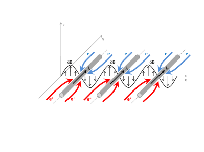
Figure 6: Sketch of the development of the current-driven filamentation instability in 1D, with a perturbation along $x$. The current carried by the suprathermal particles, oriented along $-y$, is not indicated here. Electrons and positrons of the ambient plasma flow in opposite directions to compensate this current; if present, a magnetic fluctuation along $z$ leads to density enhancements along filaments, thereby creating a current perturbation which feeds back positively on the magnetic fluctuation.

3 Discussion

In our treatment of the instability, we have neglected the response of the plasma of suprathermal particles. This choice is dictated by simplicity, as including the response involves doubling the number of fluid variables, which renders the problem untractable. However, one should expect this approximation to be valid at maximal growth rate, since $\Im\omega$ then becomes larger than the plasma frequency of the suprathermal particles, $\omega_{\rm pb}=\xi_{\rm cr}^{1/2}\omega_{\rm p}$, with $\omega_{\rm p}$ the plasma frequency of the ambient (upstream) plasma. As the instability develops and turbulence grows, one should of course expect the orbits of these suprathermal particles to deviate from their zeroth order form given in App. A; this influence will be made more precise in the following Sec. 3.2.

3.1 Relevance to relativistic shocks

Let us now discuss why the current-driven filamentation instability is likely to play a central role in shaping the precursor, the shock and the acceleration process in the relativistic mildly magnetized regime.

Advection through the shock front provides a crucial limitation for the growth of instabilities upstream of a relativistic shock front. In the upstream plasma rest frame, this can be understood as follows: the precursor extends at most to a distance $c/(\gamma_{\rm sh}\omega_{\rm c})$ (e.g. Milosavljević & Nakar 2006, Pelletier et al. 2009), because the suprathermal particles only rotate by an amount $1/\gamma_{\rm sh}$ before being caught back by the shock front; this takes a time $t_{\rm u}\,\sim\,\gamma_{\rm sh}\omega_{\rm c}^{-1}$, but the distance between the shock front and the tip of this precursor does not exceed $t_{\rm u}(1-\beta_{\rm sh}^{2})\sim t_{\rm u}/(2\gamma_{\rm sh}^{2})$. Therefore, as measured in the upstream plasma rest frame (indicated by _|u), any instability whose growth rate $\Im\omega_{|{\rm u}}\,\lesssim\,\gamma_{\rm sh}\omega_{\rm c}$ cannot grow on the crossing time of the precursor. For the filamentation instability, $\Im\omega_{|\rm u}\,\sim\,\xi_{\rm cr}^{1/2}\omega_{\rm p}$, therefore the instability can grow only if $\gamma_{\rm sh}^{2}\sigma\xi_{\rm cr}^{-1}\,\lesssim\,1$ (Lemoine & Pelletier 2010, 2011). This indicates that mildly magnetized and/or large Lorentz factor shock waves cannot be mediated by the Weibel-filamentation instability, as mentioned in the introduction.

The present current-driven filamentation instability modifies this picture, because it grows faster than any of the other instabilities discussed in the context of relativistic shocks, and mostly because of the impact of the current on the incoming plasma in the shock front frame: as discussed in App. A and Sec. 2, if $\gamma_{\rm sh}\xi_{\rm cr}\,\gtrsim\,1$, the upstream cannot compensate the current at rest; it is therefore accelerated along $x$ to a Lorentz factor $\gamma_{{\cal R}|\rm u}\,\sim\,\gamma_{\rm sh}\xi_{\rm cr}/2$ in the upstream rest frame, and its apparent density increases by a similar amount. In the shock front frame, the incoming plasma is slowed down to velocities $\beta_{x,\rm in}\,\sim\,-(1-\xi_{\rm cr}^{2}/2)$, which means that the rest frame of the plasma effectively moves with a Lorentz factor (along $\boldsymbol{-x}$): $\gamma_{{\cal R}|\rm sh}\,\sim\,1/\xi_{\rm cr}$. This change of rest frame, relative to far infinity, strongly modifies the criterion under which the instability has or does not have time to grow. In the ${\cal R}$ frame, which defines the rest frame of the background plasma after its acceleration phase, the shock front moves with a Lorentz factor $\gamma_{{\cal R}|\rm sh}$, therefore the precursor size extends to $c/\left(\gamma_{{\cal R}|\rm sh}\omega_{\rm c}\right)$ and the timescale for a plasma mode to cross this precursor now reads

$$t_{x|{\cal R}}\,\simeq\,\frac{1}{\gamma_{{\cal R}|\rm sh}|\beta_{{\cal R}|\rm sh}|\omega_{\rm c}}\ ,$$ (39)

so that the instability can grow whenever $\Im\omega\,t_{x|{\cal R}}\,\gtrsim\,1$, or

$$\sigma\,\lesssim\,\xi_{\rm cr}^{2}\ ,$$ (40)

For typical values $\xi_{\rm cr}\,\sim\,0.1$, this implies that growth is possible up to magnetization levels $\sigma\sim 10^{-2}$, irrespective of the Lorentz factor of the shock. The latter point is of importance, because it guarantees the growth of instabilities at large $\gamma_{\rm sh}$, for which the precursor becomes very short in the upstream rest frame. This result appears compatible with recent PIC simulations, as we argue in Sec. 3.3.

Once micro-turbulence grows upstream of a relativistic collisionless shock, one may expect the Fermi process to develop (e.g. Lemoine et al. 2006, Niemiec et al. 2006) although how well it develops depends on the relative efficiency of scattering in the micro-turbulence relatively to advection in the large scale field (Pelletier et al. 2009, Lemoine & Pelletier 2010). To discuss this on quantitative grounds, we write the scattering frequency in the downstream rest frame

$$\nu_{\rm s}\,\sim\,c\lambda_{\delta B}/r_{\rm g}^{2}\,\sim\,\epsilon_{B,\rm d}\left(\lambda_{\delta B}\omega_{\rm p}/c\right)\,\omega_{\rm p}\ ,$$ (41)

$\epsilon_{B,\rm d}$ denoting an average value of the equipartition fraction of the magnetic field downstream of the shock, $\lambda_{\delta B}$ representing the coherence length of the field; the above equation holds for typical supra-thermal particles of Lorentz factor $\gamma_{\rm sh}$ in the downstream frame. As discussed in Lemoine & Pelletier (2010), scattering beats advection, hence the Fermi process develops, when

$$\nu_{\rm s}\,\gg\,\omega_{\rm c}\,\Leftrightarrow\,\sigma\,\ll\,\epsilon_{B,\rm d}^{2}\left(\lambda_{\delta B}\omega_{\rm p}/c\right)^{2}\ .$$ (42)

PIC simulations suggest $\epsilon_{B,\rm d}\,\sim\,0.01$ and $\lambda_{\delta B}\,\sim\,1-10c/\omega_{\rm p}$ with some degree of uncertainty. Nevertheless, the above result indicates that the current driven instability that we are discussing here must also play a key role in the switch-on of the Fermi process, by building up the micro-turbulence for any value of the shock Lorentz factor, up to magnetization levels as high as $\sigma\,\lesssim\,10^{-2}$.

3.2 Current-driven instability vs Weibel/filamentation

At very low magnetization levels, one must expect this current-driven filamentation to gradually disappear, once the other more standard (Weibel-filamentation, two stream etc.) instabilities can grow. To see this, consider the extreme $\sigma\,\rightarrow\,0$ limit: the Weibel/filamentation instability then grows, excites turbulence which scatters the suprathermal particles; since this turbulence has no preferred direction in the tranverse plane $(\boldsymbol{y},\boldsymbol{z})$, no net perpendicular current arises and current-driven filamentation does not take place.

At finite magnetization, the average current does not vanish, but it may be randomized by the micro-turbulence. This effect has not been taken into in the present calculations, which work at linear order and which neglect the response of the cosmic rays. In order to quantify the magnitude of the back-reaction of the turbulence on the particle trajectories, one must compare the upstream residence time derived under the assumption that microturbulence controls the scattering process with that derived assuming a coherent gyration in the background field. Furthermore, this comparison must be made upstream, in the proper frame of the micro-turbulence. In what follows, we assume that this frame corresponds to ${\cal R}$. In this ${\cal R}$ frame, the turbulent magnetic field strength $\delta B_{\cal R}\,\simeq\,\delta B/\gamma_{{\cal R}|\rm sh}$ relatively to that measured in the shock front; similarly, the typical Lorentz factor of a supra-thermal particle can be written $\overline{\gamma}_{\cal R}\,\simeq\,\gamma_{{\cal R}|\rm sh}\gamma_{\rm sh}$; the background field has a strength $B_{z|\cal R}\,\simeq\,\gamma_{{\cal R}|\rm u}B_{\rm u}$ [see Eq. (2)]. In this ${\cal R}$ frame, return to the shock takes place once the particle has been scattered by an angle $\delta\theta_{\cal R}\,\sim\,1/\gamma_{{\cal R}|\rm sh}$ (see the discussion in Milosavljević & Nakar 2006, Plotnikov et al. 2013a). If the supra-thermal particles gyrate coherently in the background electromagnetic field, return occurs on a timescale $t_{{\rm r}\omega|\cal R}\,\sim\,\delta\theta_{\cal R}/\omega_{\cal R}$, with $\omega_{\cal R}\,\simeq\,\left(\gamma_{{\cal R}|\rm u}/\overline{\gamma}_{\cal R}\right)\omega_{\rm c}$. If micro-turbulence controls the scattering with scattering frequency $\nu_{\rm s|\cal R}\,\sim\,c\lambda_{\delta B|\cal R}/r_{\rm g|\cal R}^{2}$, return takes place on a timescale $t_{{\rm r}\nu|\cal R}\,\sim\,\delta\theta_{\cal R}^{2}/\nu_{\rm s|\cal R}$. Comparing the two timescales leads to a critical magnetization level:

$$\sigma_{\rm c}\,\sim\,\xi_{\rm cr}^{2}\,\epsilon_{B,\rm u}^{2}\,\left(\lambda_{\delta B|\cal R}\omega_{\rm p}/c\right)^{2}\ .$$ (43)

The quantity $\epsilon_{B,\rm u}$ denotes the typical level of micro-turbulence, usptream of the shock, as measured in the shock front frame. The factor $\xi_{\rm cr}$ appears in this formula because the comparison has been made in the ${\cal R}$ frame. If the upstream magnetization $\sigma\,\lesssim\,\sigma_{\rm c}$, then micro-turbulent scattering efficiently randomizes the trajectories in the shock front plane, hence the perpendicular current as well. Conversely, if $\sigma\,\gtrsim\,\sigma_{\rm c}$, the return trajectories maintain their coherence, hence the current-driven instability develops efficiently.

An interesting question is what happens at large Lorentz factors and low magnetization levels $\sigma\,\ll\,\sigma_{\rm c}$, where feedback from the turbulence should not be neglected, but where the Weibel-filamentation instability does not have time to grow (in the absence of slow-down of the plasma, see below). This area of parameter space corresponds to $\sigma\gamma_{\rm sh}^{2}\xi_{\rm cr}^{-1}\,\gtrsim\,1$ and $\sigma\,\lesssim\,\sigma_{\rm c}$. Our analysis suggests that the current-driven instability must develop at the tip of the precursor, where the turbulence is sufficiently weak that its back-reaction can be neglected. Furthermore, the deceleration of the plasma, which results from current compensation, now allows the Weibel/filamentation instability to grow: Eq. (39) indicates that growth becomes possible in the ${\cal R}$ frame whenever $\sigma\,\lesssim\,\xi_{\rm cr}^{3}$. This instability may then step over closer to the shock front, where the back-reaction of the turbulence strongly randomizes the return trajectories of the supra-thermal particles.

Nevertheless, one expect the precursor to be shaped by the size $c/\omega_{\rm c}$ if the current-driven instability shapes the precursor, or even the tip of the precursor: beyond that length scale, the turbulence must die away quickly, because the plasma has not yet slowed down and instabilities cannot grow there; inside the precursor, one may expect some form of equilibrium to be reached between the level of the turbulence, the slow-down of the plasma and the growth rate of the instabilities. Its detailed study lies beyond the present work.

This description contrasts with what one expects in the region of parameter space in which the Weibel-filamentation instability can grow without the slow-down imposed by the current, i.e. $\sigma\gamma_{\rm sh}^{2}\xi_{\rm cr}^{-1}\,\lesssim\,1$ and $\sigma\,\ll\,10^{-5}$. There, as discussed above, the current is mostly randomized by the near isotropicity of the trajectories of suprathermal particles in the shock front plane. In this limit, the precursor extends to a scale $\epsilon_{B}^{-1}\left(\lambda_{\delta B}\omega_{\rm p}/c\right)^{-1}\,c/\omega_{\rm p}$, smaller than $c/\omega_{\rm c}$, since the return of suprathermal particles is controlled by the scattering in the small-scale turbulence (Milosavljević & Nakar 2006, Pelletier et al. 2009). This situation actually matches the unmagnetized shock limit; hence, one may expect to find a universal precursor profile, independent of the magnetization parameter. The detailed discussion of the profile in this regime is also left open for further study.

3.3 Comparison to PIC simulations

Particle-in-cell simulations offer valuable tools to probe the physics of relativistic collisionless shock waves. So far, most studies have discussed the unmagnetized or strongly magnetized limit and few have addressed the mild magnetization regime, of interest here. We thus confront our findings to the recent simulations of Sironi et al. (2013), which have explored the regime of moderate magnetizations $\sigma\,=\,10^{-4}\rightarrow 10^{-2}$ at various shock Lorentz factors $\gamma_{\rm sh}\,=\,5\rightarrow 200$. Such simulations are performed in the downstream plasma rest frame, which does not differ much from the shock rest frame. In this rest frame, the slow-down of the plasma along $\boldsymbol{x}$ is difficult to measure, because the relative modification of $u_{x,\rm in}$ is only of order $\xi_{\rm cr}$, see App. A.

However, their Fig. 7 is particular interesting, because it reveals a precursor whose profile does not depend on $\sigma$, provided one rescales the distances by $\sigma^{1/2}\,=\,\omega_{\rm c}/\omega_{\rm p}$, i.e. provided the distances are expressed in units of $c/\omega_{\rm c}$. It is actually possible to infer directly from their figure the typical scale height of the precursor, $\sim 2c/\omega_{\rm c}$, with a rough exponential dependence. For the parameters probed in this figure, $\gamma_{\rm sh}=21$ ($=\sqrt{2}\gamma_{0}$ with their $\gamma_{0}=15$) and $\sigma=10^{-4}\rightarrow 10^{-3}$, the Weibel-filamentation instability cannot grow without the slow-down of the plasma imparted by the current-driven filamentation. Therefore these simulations directly probe the region of parameter space discussed above, in which the current-driven filamentation instability plays the central role. The structure of the precursor conforms well to the expectations, with a size $\sim c/\omega_{\rm c}$.

In their Fig. 5, these authors show the magnetic structure of the precursor in 3D simulations for similar parameters; the magnetic field appears to be structured in sheets parallel to the $x-y$ plane rather than filaments oriented along $\boldsymbol{x}$, which would be expected for a standard Weibel/filamentation instability. Finally, they report no dependence on the shock Lorentz factor, whereas a rather strong dependence is expected if the Weibel-filamentation instability alone shapes the precursor: as the line $\sigma\gamma_{\rm sh}^{2}\xi_{\rm cr}^{-1}=1$ is crossed, one expects to transit in a region in which the Weibel-filamentation instability can no longer grow. This independence relative to the Lorentz factor directly results from the slow-down imposed by the current compensation in the $\gamma_{\rm sh}\xi_{\rm cr}\,\gg\,1$ limit: inside the precursor, everything happens as if the shock were moving relative to upstream with the Lorentz factor $\gamma_{{\cal R}|\rm sh}\,\sim\,1/\xi_{\rm cr}$, so that all memory of the initial $\gamma_{\rm sh}$ is lost.

These trends strongly suggest that the present current-driven filamentation instability shapes the precursor and the shock of weakly magnetized ($\sigma\,\ll\,1$) relativistic shock waves.

Finally, the picture that we have elaborated in Sec. 3.1 also allows to understand, at least qualitatively, the results of Sironi et al. (2013) concerning the development of Fermi acceleration. Their simulations indicate that Fermi acceleration develops for any value of the shock Lorentz factor, for magnetization levels $\sigma\,\lesssim\,10^{-5}$. This conforms well with Eq. (42) and the discussion in Lemoine & Pelletier (2010). There, current-driven filamentation can grow, irrespectively of the shock Lorentz factor; it builds up turbulence and, because $\sigma\,\lesssim\,10^{-5}$, scattering in the micro-turbulence downstream of the shock front beats advection, hence the Fermi process develops. At larger values of $\sigma$, the same simulations indicate that Fermi acceleration develops in a restricted dynamic range, with a maximum energy scaling as $\sigma^{-1/4}$. Equation (42), taken at face value, would indicate that Fermi acceleration should not develop in this limit. However, this argument assumes a homogeneous micro-turbulence downstream of the shock, of strength $\epsilon_{B,\rm d}$, whereas the micro-turbulence seen in PIC simulations actually decreases away from the shock front. If the law of evolution of $\epsilon_{B}$ were known, one could improve on Eq. (42) by comparing the scattering time in this evolving micro-turbulence and the gyration time in the background field. In the absence of such a well-defined law, one can nevertheless understand on a qualitative level the scaling of the maximal energy: as the magnetization increases beyond $10^{-5}$, the condition $\sigma\,\lesssim\,\epsilon_{B,\rm d}^{2}$ remains true only in a finite layer close to the shock front; since the scattering length-scale evolves as the square of the particle energy, the restricted size of this layer leads to the existence of a maximal energy. Let us note, that if this layer were of infinite extent, there would nevertheless be a maximal energy, scaling as $\sigma^{-1/2}$, as dicussed in Pelletier et al. (2009).

3.4 Consequences

The above discussion directly impacts our understanding of shock structuration and of particle acceleration. For instance, Sironi et al. (2013) argue that in front of the shock, there exists a layer of size $\sim c/\omega_{\rm c}$ filled with Weibel turbulence at a level $\epsilon_{B}\,\sim\,10^{-2}$; this observation is based on the simulations reported above, in the range $\sigma=10^{-4}\rightarrow 10^{-2}$. According to the above discussion, this layer actually reflects the constrained growth of current-driven filamentation and Weibel- filamentation instabilities in the precursor, whose size is set by the current profile, which extends on $c/\omega_{\rm c}$, and the turbulence is not of Weibel origin.

These authors then extrapolate their results to the regime of low magnetization $\sigma\,\ll\,10^{-5}$ to discuss the maximal energy of particles accelerated at relativistic shocks. The above arguments indicate that such an extrapolation is not justified, because the physics of the precursor are likely to change as one transits from the region controlled by the current-driven filamentation instability to that controlled solely by the Weibel-filamentation mode. In particular, as $\sigma\rightarrow 0$, the diverging scale $c/\omega_{\rm c}$ must decouple and one expects the precursor profile to be entirely controlled by the micro-turbulence, as in the unmagnetized limit. The above discussion indicates that this transition takes place close to the line $\sigma\gamma_{\rm sh}^{2}\xi_{\rm cr}^{-1}\,\sim\,1$ and $\sigma\,\sim\,10^{-5}$ to $10^{-4}$; for $\gamma_{\rm sh}=21$ as used in these simulations, both limits reduce to the latter $\sigma\,\sim\,10^{-5}$ to $10^{-4}$.

4 Conclusions

This work reports on a new current-driven filamentation instability usptream of a magnetized relativistic collisionless shock front. As viewed in the shock front frame, the suprathermal particles, which are reflected on the shock front, or accelerated at the shock, gyrate around the perpendicular magnetic field in the shock precursor, thereby depositing a strong current $j_{\rm cr}\,\sim\,\xi_{\rm cr}\gamma_{\rm sh}\,n_{\rm u}\,e\,c$, which is both perpendicular to the magnetic field and to the shock normal. As the incoming plasma enters the precursor, it seeks to compensate this current within a few skin depth scales. If $\xi_{\rm cr}\gamma_{\rm sh}\,\gtrsim\,1$, which is a likely situation for highly relativistic shocks, the incoming plasma cannot compensate this current in the upstream rest frame; it is thus accelerated to a large Lorentz factor $\sim\xi_{\rm cr}\gamma_{\rm sh}/2$ (relative to far upstream), which increases the apparent density of the plasma by a similar factor; particles then drift at relativistic velocities in the perpendicular direction to achieve current compensation, electrons and positrons drifting in opposite directions. In the shock front rest frame, the incoming plasma is decelerated along the shock normal at the same time as it is accelerated in this perpendicular direction.

As we have argued, this current destabilizes a combination of the high frequency branch of the extraordinary mode and of the acoustic mode along the magnetic field. In a 2D configuration, in which one neglects perturbations along the direction of the current, this instability bears some resemblance to the Weibel-filamentation instability. However, in the present case, the electromagnetic perturbation couples to a density fluctuation, not to a charge fluctuation, because the counterstreaming electrons and positrons carry opposite charges. This leads to the formation of current filaments of a same polarity, all currents being oriented so as to compensate the cosmic ray current induced in the precursor. We find that this instability has a very fast growth rate, of order $\Im\omega\,\sim\,\beta_{y}\,\omega_{\rm p}$ on skin depth scales, with $\beta_{y}\,\sim\,1$ the drift velocity. This instability is likely to play a key role in shaping the precursor of weakly magnetized relativistic collisionless shocks, in which the growth of other instabilities is very often impeded by the fast transit across the precursor.

In particular, we have shown that this instability can grow at any value of the Lorentz factor, provided the magnetization parameter $\sigma\,\lesssim\,\xi_{\rm cr}^{2}\,\sim\,10^{-2}$. The relative independence to the Lorentz factor of the shock, which controls the size of the precursor $c/(\gamma_{\rm sh}\omega_{\rm c})$ (upstream rest frame), stems from the deceleration that the incoming plasma suffers inside the precursor: the relative Lorentz factor between the shock front frame and the rest frame of the plasma now falls to $\gamma_{{\cal R}|\rm sh}\,\sim\,1/\xi_{\rm cr}$, independent of $\gamma_{\rm sh}$. In this picture, the shock foot plays the role of a buffer that transforms the interaction with the fast incoming flow into a more moderate regime, depending on the parameter $\xi_{\rm cr}$, over a well defined distance $\xi_{\rm cr}c/\omega_{\rm c}$ (in the instantaneous rest frame of the incoming plasma).

In previous studies, we have argued that the filamentation, oblique two stream modes etc., can grow only at small values of $\sigma$ and moderate values of $\gamma_{\rm sh}$, e.g. such that $\sigma\gamma_{\rm sh}^{2}\xi_{\rm cr}^{-1}\,\lesssim\,1$ for the Weibel-filamentation mode (Lemoine & Pelletier 2010, 2011). Otherwise, the incoming plasma transits faster across the precursor than a growth time of the instability. Therefore, the current-driven filamentation instability emerges as the leading instability outside this region of parameter space. At very low magnetizations, $\sigma\,\ll\,10^{-5}$, and in the region where the standard filamentation mode can grow, the current-driven filamentation instability should gradually disappear, as the turbulent small scale electromagnetic fields randomize the return trajectories of the suprathermal particles in the shock front plane. In this limit, one transits to the unmagnetized limit, in which the precursor size is no longer controlled by the background magnetic field, but by the profile of the micro-turbulence.

Outside this region, up to $\sigma\,\sim\,10^{-2}$, the current driven filamentation instability is likely to play a dominant role. The interesting physics of the shock at low magnetizations and at Lorentz factor so large that the standard Weibel-filamentation mode cannot grow, deserves close scrutiny. In this region, the current filamentation instability can grow in the absence of strong microturbulence; however the very growth of this instability and of the filamentation mode, thanks to the deceleration of the plasma, builds up the small scale turbulence, which then back reacts on the current profile. The profile of the precursor in this regime is left open for further study.

Our analysis at linear level indicates that the growth rate of the current-driven filamentation instability is maximal on plasma skin depth scales. This does not affect previous results concerning the maximal energy of accelerated particles, which assume micro-turbulence set on skin depth scales, e.g. Kirk & Reville (2010), Bykov et al. (2012), Plotnikov et al. (2013a).

Appendix A Profile of the precursor

We construct here the profile of the precursor in the cold plasma limit, in the shock rest frame. We seek here a 1D zeroth order stationary solution of the shock precursor, with $\partial_{t}\,=\partial_{y}\,=\,\partial_{z}\,=\,0$, as dictated by the geometry of the problem. The perturbation of this solution leads to the linear system discussed in Sec. 2.1 and App. B. As discussed in Sec. 2, the zeroth order solution is characterized by the profile of the magnetic field $\boldsymbol{B}\,=\,B_{z}\,\boldsymbol{z}$, the convective electric field $\boldsymbol{E}\,=\,E_{y}\,\boldsymbol{y}$, and the fluid four-velocities of the various species.

Note that the $x-$component of the current density vanishes for both incoming particles and for suprathermal particles, as a consequence of the stationary state: current conservation $\partial_{\mu}j^{\mu}_{\alpha}\,=\,0$ for any species $\alpha$ implies the conservation law $\partial_{x}j^{x}_{\alpha}\,=\,0$; since the $x-$component of the current density of incoming particles, summed over electrons and positrons, vanishes as $x\rightarrow+\infty$, it also vanishes in the precursor, and similarly for the suprathermal particles. As particles gyrate in the $(\boldsymbol{x},\boldsymbol{y})$ plane, we set $u_{\alpha}^{z}\,=\,0$, hence $j_{z,\alpha}\,=\,0$ for all species.

Furthermore, we do not expect any non-zero $E_{x}$ component to emerge inside the precursor because of the charge symmetry of the pair plasma. One can check that the above solution is self-consistent. In particular, the magnetic field does not possess other components, as a result of $\boldsymbol{\nabla}\cdot\boldsymbol{B}\,=0\,$, $\partial_{y}\,=\,\partial_{z}\,=\,0$ and $j_{z}\,=\,0$.

A.1 Simplified MHD model

In Sec. 2, we provide a relativistic two-fluid description of the instability, the term two-fluid referring to the electrons and positrons of the incoming background plasma. This description thus extends beyond any MHD picture of the instability, up to the inertial scale of the pair plasma. Nevertheless, it is instructive to describe briefly the structure of the precursor in an ideal MHD picture, in which one assumes that the magnetic field remains frozen in the plasma all throughout the precursor.

Treating the suprathermal particle component as a tenuous fluid carrying a current density $\boldsymbol{j_{\rm cr}}\,=\,j_{y,\rm cr}\,\boldsymbol{y}$, with $j_{y,\rm cr}\,=\,-\gamma_{\rm sh}\xi_{\rm cr}n_{\rm u}ec$, the electric field is fixed through the frozen-in condition:

$$E_{y}\,=\,\overline{\beta}_{x,\rm in}B_{z}\ ,$$ (44)

with $\overline{\beta}_{x,\rm in}$ denoting the center-of-mass $3-$velocity $x-$component of the incoming plasma. Then $\boldsymbol{\nabla\times E}\,=\,0$ imposes $\partial_{x}\left(\overline{\beta}_{x,\rm in}B_{z}\right)\,=\,0$, or

$$\overline{\beta}_{x,\rm in}B_{z}\,=\,\beta_{\rm sh}B_{\infty}\ ,$$ (45)

with $B_{\infty}\,=\,\gamma_{\rm sh}B_{\rm u}$. To keep the analysis brief, here, we assume $\gamma_{\rm sh}\xi_{\rm cr}\,\ll\,1$, meaning that the velocity of the electrons/positrons of the background plasma along the $\boldsymbol{y}$ direction is much smaller than $c$. This allows to set $\overline{\beta}_{x,\rm in}\,\simeq\,\overline{u}_{x,\rm in}/\left(1+\overline{u}_{x,\rm in}^{2}\right)^{1/2}$ in the above equations, with $\overline{u}_{x,\rm in}$ the $x-$component of the center-of-mass $4-$velocity.

The current density flowing in the incoming background plasma is itself fixed through

$$j_{y,\rm in}\,=\,-j_{y,\rm cr}-\frac{c}{4\pi}\partial_{x}B_{z}\ .$$ (46)

Particle number conservation $\partial_{x}\left(n_{\rm u}u_{x}\right)\,=\,0$ and energy-momentum conservation in the cold plasma limit then lead to the equation:

$$n_{\rm u}m_{e}c^{2}\overline{u}_{x,\rm in}\partial_{x}\overline{u}_{x,\rm in}\,=\,\frac{1}{c}j_{y,\rm in}B_{z}\ .$$ (47)

This equation of motion becomes an equation for $\overline{u}_{x,\rm in}$, once Eqs. (45) and (46) have been taken into account. This equation can be rewritten in the following compact form:

$$\left[1-\frac{\beta_{\rm sh}^{2}\gamma_{\rm sh}^{2}\overline{\beta}_{x,\rm in}^{2}}{\overline{u}_{x,\rm in}^{4}}\sigma\right]\,\overline{\beta}_{x,\rm in}\overline{u}_{x,\rm in}\partial_{x}\overline{u}_{x,\rm in}\,=\,\beta_{\rm sh}\gamma_{\rm sh}\xi_{\rm cr}\frac{\omega_{\rm c}}{c}\ .$$ (48)

In this equation, we have used the definition of the magnetization parameter, Eq. (13) and $\omega_{\rm c}\,=\,eB_{\rm u}/(m_{e}c)\,=\,eB_{\infty}/\left(\gamma_{\rm sh}m_{e}c\right)$. Equation (48) is particularly useful, because it allows to obtain a quick estimate of the slow-down of the plasma due to the Lorentz force: one first notes that the second term in the brackets, which originates from the uncompensated part of the current in the precursor, is much smaller than unity, and can be safely neglected; then, one finds that between entry into the precursor and shock crossing, the variation of $\overline{u}_{x,\rm in}$ reads

$$\Delta\overline{u}_{x,\rm in}\,\simeq\,-u_{\infty}\xi_{\rm cr}\ ,$$ (49)

with $u_{\infty}\,=\,\gamma_{\rm sh}\beta_{\rm sh}$; note that the scale of variation is set by the precursor size $c/\omega_{\rm c}$. Assuming now that the transverse $3-$velocity of electrons and positrons, along $\boldsymbol{y}$, is of order $\pm\gamma_{\rm sh}\xi_{\rm cr}$, one can check that the $3-$velocity $\overline{\beta}_{x,\rm in,0}$ close to the shock front is of the order of

$$\overline{\beta}_{x,\rm in,0}\,\simeq\,\beta_{\rm sh}\,\left(1-\frac{\xi_{\rm cr}^{2}}{2}\right)\ .$$ (50)

These results will remain true in the following multi-fluid description, even at large values of the quantity $\gamma_{\rm sh}\xi_{\rm cr}$. In the above MHD model, $\partial_{x}B_{z}/B_{z}\,=\,-\partial_{x}\overline{\beta}_{x,\rm in}/\overline{\beta}_{x,\rm in}$, therefore the above scalings allow to derive an estimate of $(c/4\pi)\partial_{x}B_{z}$, which characterizes the departure from current compensation in the precursor:

$$\left|\frac{4\pi j_{y,\rm cr}}{c\,\partial_{x}B_{z}}\right|\,\approx\,\frac{1}{\xi_{\rm cr}\sigma}\,\gg\,1\ ,$$ (51)

indicating that the current is indeed compensated to very high accuracy in the precursor.

A.2 Multi-fluid model

We now turn to a more exhaustive multi-fluid model of the precursor, which is necessary to construct the steady state on which the linear analysis of Sec. 2 relies. In particular, we relax the frozen-in condition of the magnetic field inside the precursor and we follow the kinematics of the various particle populations along the $\boldsymbol{y}$ direction. Of course, well outside the precursor, one still assumes $E_{y}\,=\,\beta_{\rm sh}B_{z}$, corresponding to the assumption of zero electric field in the rest frame of the background plasma as $x\rightarrow+\infty$.

We consider the following populations of particles: the incoming particles, denoted by the subscript _in, and the suprathermal particle population, which we divide into two sub-populations, those moving toward $\boldsymbol{+x}$ from the shock front up to the tip of the precursor (subscript _r+) and those moving toward $\boldsymbol{-x}$ from the tip of the precursor toward the shock front (subscript _r-). We set the shock front at $x=0$ and the tip of the precursor at $x_{1}$. All throughout this section, we denote by $u^{\mu}_{\alpha}$ the four-velocity of the positron component of species $\alpha$, with $\alpha\,\in\,\left({\rm in},{\rm r+},{\rm r-}\right)$. As discussed in Sec. 2, the $x-$ components of the $4-$velocities of the electrons match those of the positrons, while the $y-$components are opposite.

Alsop & Arons (1988) have described the structure of the precursor of a strongly magnetized relativistic shock; they do so by solving the fluid and Maxwell equations with one population of incoming particles, which gyrate in the compressed magnetic field. The present description is slightly different: we set a boundary at $x=0$, corresponding to the shock transition, into which the incoming population flows and out of which the suprathermal particle population emerges, with no specific relation between these two populations.

In the cold plasma limit, the coherent rotation of the suprathermal particles at the tip of the precursor implies $\beta_{x,\rm r\pm}(x_{1})=0$, therefore $n_{\rm r\pm}(x_{1})\,\rightarrow\,+\infty$, and consequently $|j_{y}(x_{1})|\,\rightarrow\,\infty$. This singular behaviour disappears of course when warm plasma effects are introduced. Indeed, the suprathermal particle population should be described in the present shock rest frame as a relativistically hot plasma with mean Lorentz factor $\sim\gamma_{\rm sh}$ and roughly isotropic distribution function. Such effects are discussed in the next App. A.3. The cold plasma approximation, which we use here, has the advantage of providing quantitative estimates for the various quantities used in the manuscript.

The electromagnetic profile is thus determined by $B_{z}\,\equiv\,\gamma_{\rm sh}B_{\rm u}(1+b)$, by the current $j_{y}$ and the four-velocities of the respective fluids. This profile of the precursor can be solved as a shooting problem, with three parameters to be determined by the boundary conditions: $b_{1}$, $\gamma_{\rm r1}$, corresponding respectively to the deviation from $\gamma_{\rm sh}B_{\rm u}$, the Lorentz factor of suprathermal particles at the tip of the precursor, and $x_{1}$. The boundary conditions are:

$$u_{x,\rm r+,0}\,=\,u_{\rm sh}\ ,\quad u_{y,\rm r+,0}\,=\,0\ ,$$

$$n_{\rm r-,0}u_{y,\rm r-,0}\,=\,-n_{\rm in,0}u_{y,\rm in,0}\ .$$ (52)

The first two conditions specify the inital data for the suprathermal particle population: we have chosen here a normal incidence to the shock front and a Lorentz factor $\gamma_{\rm sh}$, as expected at relativistic shocks. The third condition imposes a vanishing net flux of particles along the shock front in the $\boldsymbol{y}$ direction.

In the cold plasma limit, and under the stationary state approximation $\partial_{t}\,=\,0$, the fluid equations $\partial_{\mu}\left(n_{\alpha}u_{\alpha}^{\mu}\right)\,=\,0$ and $\partial_{\mu}T^{\mu\nu}_{\alpha}\,=\,+e\,n_{\alpha}u^{\mu}_{\alpha}F^{\nu}_{\,\,\mu}$ (for the positron components) read:

$$\partial_{x}\left(n_{\alpha}u_{\alpha}^{x}\right) \,=\, 0\ ,$$

$$\beta_{x,\alpha}\,\partial_{x}u^{x}_{\alpha} \,=\, \frac{e}{m_{e}}\beta_{\alpha,y}B_{z}\ ,$$

$$\beta_{x,\alpha}\,\partial_{x}u^{y}_{\alpha} \,=\, \frac{e}{m_{e}}\left(E_{y}-\beta_{\alpha,x}B_{z}\right)\ ,$$

$$\beta_{x,\alpha}\,\partial_{x}\gamma_{\alpha} \,=\, \frac{e}{m_{e}}\beta_{y,\alpha}E_{y}\ .$$ (53)

Here, $\gamma_{\alpha}\,\equiv\,u^{0}_{\alpha}$. For the various species, the continuity equations imply that at each point: $n_{\rm in}u_{x}\,=\,n_{\infty}u_{\infty}$ with $u_{\infty}=\gamma_{\rm sh}\beta_{\rm sh}<0$, $n_{\rm r+}u_{x,\rm r+}\,=\,\xi_{\rm cr}n_{\infty}u_{\rm x,r+,0}$, $n_{\rm r-}u_{x,\rm r-}\,=\,-\xi_{\rm cr}n_{\infty}u_{\rm x,r+,0}$. The quantity $n_{\infty}$ represents the proper particle density as $x\rightarrow+\infty$, while $u_{x,r\pm,0}$ represents the $x-$component of the 4-velocity of species $r\pm$ at the shock front.

Complemented with Ampère’s law $\partial_{x}B_{z}\,=\,-4\pi j_{y}/c$, the system Eq. (53) may then be rewritten:

$$\beta_{x,\alpha}\partial_{x}\beta_{x,\alpha} \,=\, \frac{\omega_{\rm L,\alpha}}{c}\left[(1+b)-\beta_{x,\alpha}\beta_{\rm sh}\right]\beta_{y,\alpha}\ ,$$

$$\beta_{x,\alpha}\partial_{x}\beta_{y,\alpha} \,=\, \frac{\omega_{\rm L,\alpha}}{c}\left[\beta_{\rm sh}\left(1-\beta_{y,\alpha}^{2}\right)-\beta_{x,\alpha}(1+b)\right]\ ,$$

$$\beta_{x,\alpha}\partial_{x}\gamma \,=\, \frac{\omega_{\rm L,\alpha}}{c}\gamma\beta_{y,\alpha}\beta_{\rm sh}\ ,$$

$$\partial_{x}b \,=\, -\frac{\omega_{\rm c}}{\sigma\gamma_{\rm sh}n_{\infty}c}\left(n_{\rm in}u_{y,\rm in}+n_{\rm r+}u_{y,\rm r+}+n_{\rm r-}u_{y,\rm r-}\right)\ ,$$

with $\omega_{\rm L,\alpha}\,\equiv\,e\gamma_{\rm sh}B_{\rm u}/(\gamma_{\alpha}mc)\,=\,\omega_{\rm c}\gamma_{\rm sh}/\gamma_{\alpha}$, in terms of $\omega_{\rm c}\,\equiv\,eB_{\rm u}/(mc)$ the upstream cyclotron frequency, which sets the spatial scale $c/\omega_{\rm c}$ of the precursor. As discussed above, $u_{y,\rm in}$, $u_{y,\rm r+}$ and $u_{y,\rm r-}$ represent the $y-$components of the $4-$velocities of the incoming, suprathermal ${\rm r+}$ and ${\rm r-}$ positron components respectively. The last equation for $b$ implicitly uses the fact that the $y-$velocities of electrons are opposite to those of the positrons, for both incoming and suprathermal particles, hence their $y-$current densities add up; the magnetization $\sigma$ is defined in Eq. (13). This last equation holds in the shock precursor where the various populations mix.

Given the above three parameters $b_{1}$, $\gamma_{\rm r1}$ and $x_{1}$, these fluid equations must then be matched to the boundary conditions; this determines the profile of the precursor.

Numerical examples of the profile are represented in Fig. 7. We have set $\sigma=0.01$, $\xi_{\rm cr}=0.1$ and $\gamma_{\rm sh}=10^{3}$, but the profile does not depend on $\gamma_{\rm sh}$ in the ultra-relativistic limit; it is entirely controlled by $\sigma$ and $\xi_{\rm cr}$.

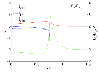
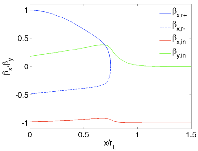
Figure 7: Structure of the precursor for $\sigma=0.01$, $\xi_{\rm cr}=0.1$ and $\gamma_{\rm sh}=1000$ ($r_{\rm L}\,\equiv\,c/\omega_{\rm c}$). Top panel: spatial profiles of the $y-$current carried by the suprathermal particle population in units of $en_{\rm u}c$ (in blue), and of the compensating current carried by the inflowing ambient plasma (in red); in green, the spatial profile of the perturbed magnetic field $b=B_{z}/B_{z,0}-1$. Bottom panel: spatial profiles of the $x-$velocities of the suprathermal particle population (in blue), of the inflowing background plasma (in red), and of the $y-$velocity of the background plasma positrons (in green).

One can obtain an approximation to the above profile as follows. In the vicinity of $x_{1}$, $n_{\rm r\pm}(x)\,\gg\,n_{\rm in}(x)$, therefore the incoming particle contribution to Ampère’s law can be neglected. Furthermore, one can approximate the motion of r+ particles close to $x_{1}$ as uniform deceleration, implying $\beta_{x}\,\simeq\,\left[2|\dot{\beta}_{x}(x_{1})|(x-x_{1})\right]^{1/2}$, with $|\dot{\beta}_{x}(x_{1})|\,=\,\omega_{\rm L1}(1+b_{1})\beta_{y,\rm r+}(x_{1})$ given that $\beta_{x}(x_{1})=0$, and $\omega_{\rm L1}\,\equiv\,\omega_{\rm L,r+}(x_{1})$. This allows to determine the singular profile of the density close to $x_{1}$, using the continuity equation. Plugging this result and the similar estimate for r- particles into Ampère’s law, one derives

$$b\,\simeq\,b_{1}\,\left[1+\frac{\xi_{\rm cr}}{\sigma}\frac{|\beta_{x,\rm r+}(0)|\sqrt{\beta_{y,\rm r+}(x_{1})}}{\sqrt{2}(1+b_{1})^{1/2}b_{1}}\omega_{\rm L1}^{1/2}\left(x-x_{1}\right)^{1/2}\right]\ .$$ (55)

The term in the brackets determine the scale over which $b$ varies close to $x_{1}$, $\Delta x\,\sim\,\sigma^{2}\xi_{\rm cr}^{-2}b_{1}^{3}c/(\sqrt{2}\omega_{\rm L1})$. Using Ampère’s law with $\partial_{x}b\,\sim\,b_{1}/\Delta x$, $\omega_{\rm L1}\,\sim\,\omega_{\rm c}$ and assuming $b\,\gg\,1$ leads to

$$b_{1}\,\sim\,\left(\frac{\xi_{\rm cr}}{\sigma}\right)^{1/2}\ .$$ (56)

The above turns out to provide the correct scaling seen in the numerical calculations. In turn, this leads to $\Delta x\sim\sigma^{1/2}\xi_{\rm cr}^{-1/2}c/\omega_{\rm c}\,\sim\,\xi_{\rm cr}^{-1/2}c/\omega_{\rm p}$: current compensation takes place on skin depth scales, as anticipated in Lemoine & Pelletier (2011).

Outside the precursor, the field goes down to its asymptotic far upstream value on skin depth scales as well. Equations (LABEL:eq:prec) can be used in this region, with $n_{\rm r\pm}\rightarrow 0$ in Ampère’s law. As discussed in Alsop & Arons (1988), the system then admits the two integrals of motion

$$\gamma_{\rm in} \,=\, \gamma_{\rm sh}\left(1-\sigma b\right)\ ,$$

$$u_{x,\rm in} \,=\, u_{\infty}\left[1-\frac{\sigma}{2\beta_{\rm sh}^{2}}b\left(b+2\right)\right]\ .$$ (57)

These two integrals, combined with Eqs. LABEL:eq:prec allow to derive the following equation for the profile of $b$:

$$\partial_{x}b\,=\,-\frac{\omega_{\rm c}}{\sqrt{\sigma}c}\frac{\left[b^{2}-\sigma b^{2}/(\gamma_{\rm sh}^{2}\beta_{\rm sh}^{2})-\sigma b^{3}/\beta_{\rm sh}^{2}-\sigma b^{4}/(4\beta_{\rm sh}^{2})\right]^{1/2}}{1-\sigma b(b+2)/(2\beta_{\rm sh}^{2})}\ .$$ (58)

This equation reveals the length scale of the profile: $c/\omega_{\rm p}$, and allows to solve for $b$, by integrating from $b_{1}$ up to $+\infty$, then for $u_{\rm in}$.

Using the integrals of motion, one computes the typical change in Lorentz factor at the entrance into the precursor,

$$\gamma(x_{1}) \,=\, \gamma_{\rm sh}\left(1-\sqrt{\sigma\xi_{\rm cr}}\right)\ ,$$

$$u_{x,\rm in}(x_{1}) \,\simeq\, u_{\infty}\left(1-\xi_{\rm cr}/2\right)\ ,$$ (59)

$$|u_{y,\rm in}(x_{1})| \,\simeq\, -u_{\infty}\sqrt{\xi_{\rm cr}}\ .$$ (60)

The variation in Lorentz factor is small compared to that of $u_{x}$ and $u_{y}$, but the slow-down along $x$ is substantial: at $x_{1}$, the particles move at velocity $\beta_{x,\rm in}(x_{1})\,\simeq\,1-\xi_{\rm cr}/2$ in the shock front frame. This slow-down is obvious in Fig. 7.

Well inside the precursor, current compensation implies

$$|u_{y,\rm in}|\,\simeq\,\xi_{\rm cr}\gamma_{\rm sh}\ .$$ (61)

In order to derive the slow-down imparted to incoming particles, one first notes that $b\,\ll\,1$ outside the peak at the tip of the precursor, as indicated by Eqs. (55) and (56). The dynamics of incoming particles is then given by Eq. (LABEL:eq:prec) with $b\,\ll\,1$, which implies that the flow is slowed by an amount

$$\Delta u_{x,\rm in}\,\simeq\,\gamma_{\rm sh}\xi_{\rm cr}\ ,$$ (62)

between the far upstream value and the value of $u_{x,\rm in}$ well inside the precursor. This value matches that at entry into the precursor, Eq. (59), and it also matches the value obtained in the simplified MHD model, Eq. (49). This slow-down appears as a direct consequence of current compensation, which imposes a Lorentz force directed in the $\boldsymbol{+x}$ direction. In a similar way, one derives $\Delta\gamma_{\rm in}\,\sim\,-\gamma_{\rm sh}\xi_{\rm cr}$. Thus the Lorentz factor of both flows remains large after its modification by the Lorentz force. In terms of 3-velocity, this implies that $\boldsymbol{\beta}^{2}$ remains close to unity, up to $1/(2\gamma_{\rm sh}^{2})$. Using Eqs. (61) and (62), one derives the $3-$velocities well inside the precursor:

$$|\beta_{y}|\,\simeq\,\xi_{cr}\ ,$$ (63)

and, at large values of $\gamma_{\rm sh}$,

$$\beta_{x,\rm in}\,\simeq\,\beta_{\rm sh}\left(1-\xi_{\rm cr}^{2}/2\right)\ .$$ (64)

Therefore, if $\gamma_{\rm sh}\xi_{\rm cr}\,\gg\,1$, then $\beta_{x,\rm in}\,\simeq\,-\left(1-\xi_{\rm cr}^{2}/2\right)$, while $\beta_{x,\rm in}\,\simeq\,\beta_{\rm sh}$ in the opposite limit, which corresponds to negligible, sub-relativistic deceleration.

Assuming that $\gamma_{\rm sh}\xi_{\rm cr}\,\gg\,1$, the relative Lorentz factor between the shock front frame and the frame ${\cal R}$ in which the incoming is at rest along $\boldsymbol{x}$, i.e. $u_{x,\rm in|{\cal R}}\,\equiv\,0$, has fallen from $\gamma_{\rm sh}$ outside the precursor down to

$$\gamma_{{\cal R}|\rm sh}\,\simeq\,\frac{1}{\xi_{\rm cr}}\ .$$ (65)

As viewed in the upstream rest frame, the ambient plasma has been picked up by the current layer and accelerated towards $\boldsymbol{+x}$ to a Lorentz factor

$$\gamma_{{\cal R}|\rm u}\,\simeq\,\gamma_{\rm sh}\frac{\xi_{\rm cr}}{2}\quad\quad\left(\gamma_{\rm sh}\xi_{\rm cr}\,\gg\,1\right)\ .$$ (66)

Finally, in the ${\cal R}$ frame in which the ambient plasma is at rest, the particles move with velocity $|\beta_{y,{\rm in}|{\cal R}}|\,\sim\,1$ with bulk Lorentz factor $\sim\gamma_{\rm sh}\xi_{\rm cr}/2$, provided of course that $\gamma_{\rm sh}\xi_{\rm cr}\,\gg\,1$. In the opposite (weak current) limit, $\gamma_{\rm sh}\xi_{\rm cr}\,\ll\,1$, one finds $|\beta_{y,{\rm in}|{\cal R}}|\,\sim\,\gamma_{\rm sh}\xi_{\rm cr}$, $\beta_{{\cal R}|\rm u}\,\sim\,0$ and $\gamma_{{\cal R}|\rm u}\,\sim\,1$; similarly, $\gamma_{{\cal R}|\rm sh}\,\sim\,\gamma_{\rm sh}$.

A.3 Warm plasma limit

The above discussion assumed a cold plasma of returning particles, with initial momentum (on the shock surface) directed along the shock normal. Here we introduce the effects of angular dispersion of the beam of returning particles. For simplicity, we neglect the dispersion in Lorentz factor of the returning particles; this dispersion can be taken into account but it should not modify strongly the overall shape of the current profile.

The number density of returning particles at the shock front (considering $e^{+}/e^{-}$ species altogether), with momentum oriented within a solid angle element $\boldsymbol{{\rm d}\Omega_{\rm i}}$, is written ${\rm d}n_{\rm r+,i}\left(\boldsymbol{\Omega_{\rm i}}\right)$. The magnitude of the current deposited by those particles in the precursor can be written:

$${\rm d}j_{y,\rm r+}(x)\,=\,\left|\beta_{y}(x)\right|\,{\rm d}n_{\rm r+}(x,\boldsymbol{\Omega_{\rm i}})ec\ .$$ (67)

Assuming that the particle population ${\rm r-}$ deposit the same amount of current as ${\rm r+}$, and using the equation of conservation for the number density of ${\rm r+}$ particles, the total current element deposited by supra-thermal particles emitted in the $\boldsymbol{\Omega_{\rm i}}$ direction reads:

$${\rm d}j_{y}(x)\,\simeq\,2\,\frac{\left|\beta_{y,\rm r+}(x)\right|}{\beta_{x,\rm r+}(x)}\beta_{x,\rm r+,i}{\rm d}n_{\rm r+,i}(\boldsymbol{\Omega_{\rm i}})ec\ ,$$ (68)

$\beta_{x,\rm r+,i}$ denoting the initial $x-$component of the 3-velocity of $\rm r+$ particles. This equation can be simplified using the result of the previous section, which indicate that $\beta_{x,\rm r+}(x)\,\simeq\,\left|2\dot{\beta}_{x,\rm r+}(x_{1})\,(x-x_{1})\right|^{1/2}$ in the vicinity of the turning point $x_{1}$, so that most of the current ${\rm d}j_{y}(x)$ is deposited at $x_{1}$. Note that $x_{1}$ depends on the initial direction $\boldsymbol{\Omega_{\rm i}}$. We then approximate the spatial profile of the current element Eq. (68) with a delta function in $x$:

$${\rm d}j_{y}(x)\,\simeq\,{\cal A}\,\,\delta\left(x-x_{1}\right)\,{\rm d}F_{\rm r+,i}(\boldsymbol{\Omega_{\rm i}})\,e\,$$ (69)

with ${\rm d}F_{\rm r+,i}(\boldsymbol{\Omega_{\rm i}})\,=\,\beta_{x,\rm r+,i}c\,{\rm d}n_{\rm r+,i}(\boldsymbol{\Omega_{\rm i}})$ the inital flux element. The prefactor is calculated by normalizing the integrated current element along $x$ in Eq. (69) to that obtained in Eq. (68).

In order to express ${\cal A}$ as a function of the initial velocities $\beta_{x,\rm r+,i}$ and $\beta_{y,\rm r+,i}$, one needs to express the quantity $|\beta_{y,\rm r+}(x)/\beta_{x,\rm r+}(x)|$ in the vicinity of $x_{1}$ using the equations of motion. These equations of motion must be written in the upstream rest frame then Lorentz transformed to the shock frame. We compute the trajectories of the returning particles in the background electromagnetic field, neglecting in particular the perturbed component of the magnetic field; this should remain a good approximation, given that the overall effect of the angular dispersion of the beam is to spread out over the precursor length scale the current profile. One then obtains first the turning point:

$$x_{1}(\boldsymbol{\Omega_{\rm i}}) \,=\, \frac{c}{\omega_{\rm c,0}}\,\gamma_{\rm sh}^{3}\,\left(1-\beta_{\rm sh}\beta_{x,\rm r+,i}\right)$$

$$\times\left[\beta_{x,\rm i|u}\sin\varpi_{1}+\beta_{y,\rm i|u}\left(1-\cos\varpi_{1}\right)+\beta_{\rm sh}\varpi_{1}\right]\ ,$$

as a function of the upstream-frame initial velocities

$$\beta_{x,\rm i|u}\,=\,\frac{\beta_{x,\rm r+,i}-\beta_{\rm sh}}{1-\beta_{x,\rm r+,i}\beta_{\rm sh}},\quad\beta_{y,\rm i|u}\,=\,\frac{\beta_{y,\rm r+,i}}{\gamma_{\rm sh}(1-\beta_{x,\rm r+,i}\beta_{\rm sh})}\ ,$$ (71)

and the quantity $\varpi_{1}$, which is defined implicitly by:

$$\beta_{x,\rm i|u}\cos\varpi_{1}+\beta_{y,\rm i|u}\sin\varpi_{1}\,=\,-\beta_{\rm sh}\ .$$ (72)

Recall that $\beta_{\rm sh}\,<\,0$ in our present notations. The initial cyclotron frequency of the returning particles reads $\omega_{\rm c,0}\,=\,e\gamma_{\rm sh}B_{\rm u}/\left(\gamma_{0,\rm r+}mc\right)$, with $\gamma_{0,\rm r+}\simeq\gamma_{\rm sh}$ their initial Lorentz factor. One derives eventually:

$${\cal A} \,=\, 2\sqrt{2}\left(x_{1}c/\omega_{\rm c,0}\right)^{1/2}\left[\gamma_{\rm sh}(1-\beta_{\rm sh}\beta_{x,\rm r+,i})\right]^{1/2}$$ (73)

$$\quad\times\left|(\beta_{x,\rm r+,i}\sin\varpi_{1}-\beta_{y,\rm r+,i}\cos\varpi_{1})\right|^{1/2}\ .$$

Finally, the flux is normalized through $\int{\rm d}F_{\rm r+,i}(\boldsymbol{\Omega_{\rm i}})\,=\,\gamma_{\rm sh}\xi_{\rm cr}n_{\infty}c$.

In the limit $\gamma_{\rm sh}\,\rightarrow\,+\infty$, all above quantities reach finite asymptotes, as it should; we use these asymptotic values in the numerical calculation of the integral over the angular variables. One finally obtains the current profile depicted in Fig. 8.

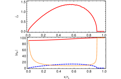
Figure 8: Upper panel: profile of $j_{y}$ (in units of $\gamma_{\rm sh}\xi_{\rm cr}n_{\infty}ec$) carried by returning particles as a function of $x/r_{\rm L}$ ($r_{\rm L}=c/\omega_{\rm c}$) in the limit $\gamma_{\rm sh}\,\gg\,1$, including the effects of angular dispersion at the shock. Lower panel: modulus of the 4-velocity components $|u_{x,\rm in}|$ (solid red), $|u_{y,\rm in}|$ (dashed blue) and $\gamma_{{\cal R}|\rm sh}$ (dotted orange); the lower panel assumes $\gamma_{\rm sh}=100$ and $\xi_{\rm cr}=0.1$.

This profile allows to estimate the velocity profile of the incoming plasma inside the foot. As in the cold plasma limit, current compensation imposes the following scalings inside the precursor

$$|u_{y,\rm in}|\,\sim\,\xi_{\rm cr}\gamma_{\rm sh}\ ,u_{x,\rm in}\,\sim\,-\left(1-\xi_{\rm cr}\right)\gamma_{\rm sh}\ ,$$ (74)

so that the relative Lorentz factor between the shock front frame and the frame ${\cal R}$ in which the incoming is at rest along $+x$ is, as before, $\gamma_{{\cal R}|\rm sh}\,\simeq\,1/\xi_{\rm cr}$ if $\gamma_{\rm sh}\xi_{\rm cr}\,\gg\,1$. Figure 8 shows a numerical calculation of the evolution of $u_{x,\rm in}$, $|u_{y,\rm in}|$ and $\gamma_{{\cal R}|\rm sh}$ inside the precursor (assuming $|b|\,\ll\,1$) for $\gamma_{\rm sh}\,=\,100$ and $\xi_{\rm cr}=0.1$, which confirms the above scalings.

Appendix B Linear system

We explicit here the linear system used to compute the dispersion relation, for reference. We rescale the time and space derivatives by $\omega_{\rm c}$ (cyclotron frequency in the upstream rest frame): $\partial_{\tilde{t}}\,\equiv\,\omega_{\rm c}^{-1}\partial_{t}$, $\partial_{\tilde{x}}\,\equiv\,c\omega_{\rm c}^{-1}\partial_{x}$ etc. We rescale all electromagnetic fields by the background value $B_{z{\cal R}}$ (e.g. $\delta\tilde{B}_{x}\,\equiv,\delta B_{x}/B_{z{\cal R}}$) and we introduce the notations: $\kappa\,\equiv\,\gamma_{{\cal R}|\rm sh}/u^{0}$, $\tilde{\beta}_{\rm s}^{2}\,\equiv\,\beta_{\rm s}^{2}/u^{0\,2}$, $\delta_{n}\,\equiv\,\delta n/n$, $\delta_{\rho}\,\equiv\,\delta\rho/n$, and we rescale $\delta u^{\mu}$ and $\Delta u^{\mu}$ by $u^{0}$, e.g. $\delta\tilde{u}^{\mu}\,\equiv\,\delta u^{\mu}/u^{0}$. This leads to the following adimensioned system

$$\partial_{\tilde{t}}\delta_{n}+\beta_{y}\partial_{\tilde{y}}\delta_{\rho}+\beta_{y}\partial_{\tilde{t}}\Delta\tilde{u}_{y}+\partial_{\tilde{x}}\delta\tilde{u}_{x}+\partial_{\tilde{y}}\delta\tilde{u}_{y}+\partial_{\tilde{z}}\delta\tilde{u}_{z} \,=\, 0$$

$$\partial_{\tilde{t}}\delta_{\rho}+\beta_{y}\partial_{\tilde{y}}\delta_{n}+\beta_{y}\partial_{\tilde{t}}\delta\tilde{u}_{y}+\partial_{\tilde{x}}\Delta\tilde{u}_{x}+\partial_{\tilde{y}}\Delta\tilde{u}_{y}+\partial_{\tilde{z}}\Delta\tilde{u}_{z} \,=\, 0$$

$$\partial_{\tilde{t}}\delta\tilde{u}_{x}+\beta_{y}\partial_{\tilde{y}}\Delta\tilde{u}_{x}+\tilde{\beta}_{\rm s}^{2}\partial_{\tilde{x}}\delta_{n}-\kappa\Delta\tilde{u}_{y}-\beta_{y}\kappa\delta\tilde{B}_{z} \,=\, 0$$

$$\partial_{\tilde{t}}\Delta\tilde{u}_{x}+\beta_{y}\partial_{\tilde{y}}\delta\tilde{u}_{x}+\tilde{\beta}_{\rm s}^{2}\partial_{\tilde{x}}\delta_{\rho}-\kappa\delta\tilde{u}_{y}-\kappa\delta\tilde{E}_{x} \,=\, 0$$

$$\partial_{\tilde{t}}\delta\tilde{u}_{y}+\beta_{y}\partial_{\tilde{y}}\Delta\tilde{u}_{y}+\tilde{\beta}_{\rm s}^{2}\partial_{\tilde{y}}\delta_{n}+\beta_{{\cal R}|\rm u}\kappa\beta_{y}\delta\tilde{u}_{y}+\kappa\Delta\tilde{u}_{x} \,=\, 0$$

$$\partial_{\tilde{t}}\Delta\tilde{u}_{y}+\beta_{y}\partial_{\tilde{y}}\delta\tilde{u}_{y}+\tilde{\beta}_{\rm s}^{2}\partial_{\tilde{y}}\delta_{\rho}+\beta_{{\cal R}|\rm u}\kappa\beta_{y}\Delta\tilde{u}_{y}$$

$$-\kappa\delta\tilde{E}_{y}+\kappa\delta\tilde{u}_{x} \,=\, 0$$

$$\partial_{\tilde{t}}\delta\tilde{u}_{z}+\beta_{y}\partial_{\tilde{y}}\Delta\tilde{u}_{z}+\tilde{\beta}_{\rm s}^{2}\partial_{\tilde{z}}\delta_{n}+\beta_{y}\kappa\delta\tilde{B}_{x} \,=\, 0$$

$$\partial_{\tilde{t}}\Delta\tilde{u}_{z}+\beta_{y}\partial_{\tilde{y}}\delta\tilde{u}_{z}+\tilde{\beta}_{\rm s}^{2}\partial_{\tilde{z}}\delta_{\rho}-\kappa\delta\tilde{E}_{z} \,=\, 0$$

$$\partial_{\tilde{t}}\delta\tilde{B}_{x}+\partial_{\tilde{y}}\delta\tilde{E}_{x}-\partial_{\tilde{z}}\delta\tilde{E}_{y} \,=\, 0$$

$$\partial_{\tilde{t}}\delta\tilde{B}_{y}+\partial_{\tilde{z}}\delta\tilde{E}_{x}-\partial_{\tilde{x}}\delta\tilde{E}_{z} \,=\, 0$$

$$\partial_{\tilde{t}}\delta\tilde{B}_{z}+\partial_{\tilde{x}}\delta\tilde{E}_{y}-\partial_{\tilde{y}}\delta\tilde{E}_{x} \,=\, 0$$

$$\partial_{\tilde{t}}\delta\tilde{E}_{x}-\partial_{\tilde{y}}\delta\tilde{B}_{z}+\partial_{\tilde{z}}\delta\tilde{B}_{y}+\frac{1}{\kappa\sigma}\Delta\tilde{u}_{x} \,=\, 0$$

$$\partial_{\tilde{t}}\delta\tilde{E}_{y}-\partial_{\tilde{z}}\delta\tilde{B}_{x}+\partial_{\tilde{x}}\delta\tilde{B}_{z}+\frac{1}{\sigma}\Delta\tilde{u}_{y}+\frac{1}{\kappa\sigma}\beta_{y}\delta_{n} \,=\, 0$$

$$\partial_{\tilde{t}}\delta\tilde{E}_{z}-\partial_{\tilde{x}}\delta\tilde{B}_{y}+\partial_{\tilde{y}}\delta\tilde{B}_{x}+\frac{1}{\kappa\sigma}\Delta\tilde{u}_{z} \,=\, 0$$

References

- [] Achterberg, A., Gallant, Y., Kirk, J. G., Guthmann, A. W., 2001, MNRAS 328, 393
- [] Achterberg, A., Wiersma, J., 2007, AA, 475, 19
- [] Achterberg, A., Wiersma, J., Norman, C. A., 2007, AA, 475, 1
- [] Alsop, D., Arons, J., 1988, Phys. Fluids, 31, 839
- [] Bret, A., Gremillet, L., Bénisti, D., 2010, Phys. Rev. E, 81, 036402
- [] Bykov, A., Gehrels, N., Krawczynski, H., Lemoine, M., Pelletier, G., Pohl, M., 2012, Space Sci. Rev., 173, 309
- [] Casse, F., Marcowith, A., Keppens, R., 2013, MNRAS, 433, 940
- [] Gallant, Y.A., Hoshino M., Langdon A.B., Arons J., Max C.E. 1992, ApJ, 391, 73
- [] Haugbølle, T., 2011, ApJ, 739, L42
- [] Hoshino, M., Arons, J., 1991, Phys. Fluids B, 3, 818
- [] Hoshino, M., Arons, J., Gallant, Y. A., Langdon, A. B., 1992, ApJ 390, 454
- [] Keshet, U., Katz, B., Spitkovsky, A., Waxman E., 2009, ApJ, 693, L127
- [] Kirk, J., Reville, B., 2010, ApJ, 710, 16
- [] Lemoine, M., Pelletier, G., Revenu, B., 2006, ApJ, 645, L129
- [] Lemoine, M., Pelletier, G., 2010, MNRAS, 402, 321
- [] Lemoine, M., Pelletier, G., 2011, MNRAS, 417, 1148
- [] Lyubarsky, Y., Eichler, D., 2006, ApJ, 647, L1250
- [] Martins, S. F., Fonseca, R. A., Silva, L. O., Mori, W. B., 2009, ApJ, 695, L189
- [] Medvedev, M. V., Loeb, A., 1999, ApJ, 526, 697
- [] Melrose, D. B., 1986, “Instabilities in Space and Laboratory Plasmas”, Cambridge University Press.
- [] Milosavljević, M., Nakar, E., 2006, ApJ, 651, 979
- [] Nekrasov, A. K., 2013, Plasma Phys. Control. Fusion, 55, 085007
- [] Niemiec, J., Ostrowski, M., Pohl, M., 2006, ApJ, 650, 1020
- [] Nishikawa, K.-I., Niemiec, J., Hardee, P. E., Medvedev, M., Sol, H., Mizuno, Y., Zhang, B., Pohl, M., Oka, M., Hartmann, D. H., 2009, ApJ, 698, L10
- [] Pelletier, G., Lemoine, M., Marcowith, A., 2009, MNRAS, 393, 587
- [] Plotnikov, I., Pelletier, G., Lemoine, M., 2013a, MNRAS, 430, 1208
- [] Plotnikov, I., Pelletier, G., Lemoine, M., Gremillet, L., 2013b, in prep.
- [] Rabinak, I., Katz, B., Waxman, E., 2011, ApJ, 736, 157
- [] Riquelme, M., Spitvkosky, A., 2010, ApJ, 717, 1054
- [] Shaisultanov R., Lyubarsky Y., Eichler D., 2012, ApJ, 744, 182
- [] Sironi, L., Spitkovsky, A., 2011, ApJ, 726, 75
- [] Sironi, L., Spitkovsky, A., Arons, J., 2013, ApJ, 771, 54
- [] Spitkovsky, A., 2008a, ApJ 673, L39
- [] Spitkovsky, A., 2008b, ApJ 682, L5
- [] Wiersma, J., Achterberg, A., 2004, AA, 428, 365