Asymptotic states and renormalization in Lorentz-violating quantum field theory

Abstract

Asymptotic single-particle states in quantum field theories with small departures from Lorentz symmetry are investigated perturbatively with focus on potential phenomenological ramifications. To this end, one-loop radiative corrections for a sample Lorentz-violating Lagrangian contained in the Standard-Model Extension (SME) are studied at linear order in Lorentz breakdown. It is found that the spinor kinetic operator, and thus the free-particle physics, is modified by Lorentz-violating operators absent from the original Lagrangian. As a consequence of this result, both the standard renormalization procedure as well as the Lehmann–Symanzik–Zimmermann reduction formalism need to be adapted. The necessary adaptations are worked out explicitly at first order in Lorentz-breaking coefficients.

I Introduction

Current understanding of physics at the fundamental level is based on two distinct theories: general relativity (GR) and the Standard Model (SM) of particle physics. It is commonly believed that these two theories arise as the low-energy limit of an underlying Planck-scale framework that consistently merges gravity and quantum mechanics. Since direct measurements at this scale are presently impractical, experimental research in this field relies largely on ultrahigh-precision searches for Planck-suppressed effects at attainable energies.

One possible effect in this context is a minute breakdown of Lorentz invariance. Lorentz symmetry is a fundamental feature of both GR and the SM, so that any observed deviation from this symmetry would imply new physics. A number of theoretical approaches to physics beyond the SM, such as strings ksp , noncommutative field theories ncqed , cosmologically varying scalar fields spacetimevarying , quantum gravity qg , random-dynamics models fn , multiverses bj , brane-world scenarios brane , and massive gravity modgrav , are believed to allow for small violations of Lorentz invariance at low energies. Searches for such violations are also motivated by the apparent fundamental character of Lorentz symmetry. Consequently, Lorentz invariance ought to be supported as firmly as possible by experimental evidence.

It is natural to expect that Lorentz-violating effects can be described within effective field theory, at least at currently attainable energies kp . The framework generally adopted in this context is the Standard-Model Extension (SME) sme ; ssb , which contains both GR and the SM as limiting cases. The additional Lagrangian terms present in the SME include all operators for Lorentz violation that are scalars under coordinate changes. The SME has constituted the basis for the analysis of numerous experimental searches for Lorentz breakdown DataTables .

Paralleling the conventional Lorentz-symmetric case, perturbative quantum-field analyses within the SME also rely on a few key theoretical concepts. Some of these, such as canonical quantization quant1 ; quant2 and renormalization Kostelecky:2001jc ; renorm ; Shapiro , have previously been studied and generalized to the SME. Another such core concept concerns the treatment of external states. They span the asymptotic Hilbert space, so their determination is of fundamental importance for perturbation theory. For example, explicit S-matrix calculations require a separate, independent determination of the external legs up to the desired order. This special status of external-leg physics is highlighted by the usual Feynman rules: external-leg corrections cannot be incorporated into the diagram for a scattering process; the rules for S-matrix calculations specifically call for “amputed” diagrams. The usual treatment of radiative corrections to external legs involves sophisticated theoretical concepts like the Källén–Lehmann representation KallenLehmann and the Lehmann–Symanzik–Zimmermann (LSZ) reduction formalism LSZ . Although a number of prior investigations have considered radiative corrections from various other perspectives (CS, ; loops, ), we are unaware of any dedicated study to generalize the Lorentz-invariant external-leg treatment to Lorentz-violating field theories.

A second need for a proper understanding of the asymptotic Hilbert space in the presence of Lorentz breakdown derives from its phenomenological importance: external-state effects govern the physics of free particles and are therefore also crucial for numerous Lorentz tests. Examples include various kinematical threshold effects in cosmic rays crays , photon birefringence and dispersion KM02 ; cphotons , collider kinematics and interferometry colliders ; hohensee ; synchrotron ; graal , and neutrino propagation neutrinos . Paralleling the conventional Lorentz-symmetric case, all previous analyses have been performed under the tacit assumption that the physics of free particles is determined by the quadratic pieces of the corresponding Lagrangian Colladay:2001wk . However, this approach disregards the self-interactions of the particle, although such effects are always present, even for asymptotic states. Consequently, they need to be considered, e.g., in any scattering process beyond tree level. In a conventional renormalizable quantum field theory (QFT), Lorentz symmetry implies that the quadratic Lagrangian can only acquire a mass shift and a field-strength factor, both of which can be treated by renormalization of existing quantities. The external QFT legs are then identical in structure to the quadratic-Lagrangian solutions, which therefore indeed describe the propagation of free particles correctly. A nonperturbative rigorous justification for this feature is given by the aforementioned LSZ reduction formalism LSZ . However, in the presence of Lorentz violation a similar line of reasoning fails, and the question regarding the determination of free-particle properties arises.

The present work is intended to initiate a theoretical investigation of these issues. In particular, we demonstrate that in the absence of Lorentz symmetry the external legs in perturbative quantum field theory exhibit a different structure than the plane-wave solutions arising from the quadratic Lagrangian GravCase . This result is in accordance with a recent work Potting:2011yj in which a generalization of the Källén–Lehmann representation for the propagator was derived for a field-theoretic model with fermions that are coupled to the same Lorentz-violating SME coefficients as the ones we are considering in this work. In fact, we will use the results obtained in Ref. Potting:2011yj to extract consistently the one-particle poles at first order in Lorentz violation. These poles define the external states of scattering amplitudes. To this end, we generalize the conventional LSZ reduction formula to include Lorentz-breaking SME corrections at linear order.

For this analysis, we restrict ourselves to a subset of the minimal SME’s electrodynamics sector for simplicity. Moreover, we are primarily focused on effects that may potentially be of phenomenological relevance and affect the usual perturbative expansion of quantum field theory. Our analysis is therefore performed at first order in SME coefficients, an approach justified on observational grounds. A future nonperturbative treatment of these issues within formal field theory would be interesting, but lies outside our present scope. Throughout, we adopt natural units $c=\hbar=1$, and our convention for the metric signature is timelike $\eta^{\mu\nu}={\rm diag}(+,-,-,-)$.

The outline of this paper is as follows. In Sec. II, our Lorentz-violating model Lagrangian is introduced and some of its properties are reviewed. Section III contains a discussion of the fermion two-point function within this model, the correct way to extract the one-particle pole in the Lorentz-violating case, and the derivation of a general formula for the corresponding spinor wave-function renormalization factor. In Sec. IV, the one-loop radiative corrections to the fermion propagator are evaluated, the one-particle pole is extracted, and the dispersion relation as well as the spinor wave-function renormalization factor are obtained. Section V extends the LSZ formalism to the Lorentz-violating case and establishes the associated Feynman expansion of the scattering matrix. In Sec. VI, the formalism developed in this paper is applied to the example of Coulomb scattering. Our summary and an outlook are contained in Sec. VII. Supplemental material is collected in various Appendixes.

II Model Basics and Scope

Our model is based on the bare gauge-invariant flat-spacetime Lagrange density for single-flavor quantum electrodynamics (QED) within the minimal SME:

$$\mathcal{L}_{\rm SME}\! = \!{\textstyle\frac{1}{2}}{\it i}\,\overline{\psi}_{B}\,{\Gamma}^{\mu}_{B}\!\!\stackrel{{\scriptstyle\;\leftrightarrow}}{{D}}\!\!{}_{\mu}^{B}\,{\psi}_{B}-\overline{\psi}_{B}\,M_{B}\,{\psi}_{B}-{\textstyle\frac{1}{4}}(F_{B})^{2}$$ (1)

$$\!{}-{\textstyle\frac{1}{4}}(k^{B}_{F})_{\mu\nu\rho\sigma}F^{\mu\nu}_{B}F^{\rho\sigma}_{B}+(k^{B}_{AF})^{\mu}A^{\nu}_{B}\tilde{F}^{B}_{\mu\nu}\;.$$

The label $B$ denotes bare quantities, $\psi_{B}$ is a Dirac spinor and $F^{B}_{\mu\nu}=\partial_{\mu}A^{B}_{\nu}-\partial_{\nu}A^{B}_{\mu}$ a gauge-field strength. We have also implemented the conventional notation for the U(1)-covariant derivative $D^{B}_{\mu}=\partial_{\mu}+ie_{B}A^{B}_{\mu}$ and for the dual field-strength tensor $\tilde{F}_{B}^{\mu\nu}={\textstyle\frac{1}{2}}\varepsilon^{\mu\nu\rho\sigma}F^{B}_{\rho\sigma}$. The Lorentz-violating effects are contained in the quantities $(k^{B}_{F})_{\mu\nu\rho\sigma}$ and $(k^{B}_{AF})^{\mu}$ as well as in the generalized gamma matrices $\Gamma^{\mu}_{B}$ and the generalized mass matrix $M_{B}$. The latter are given by the explicit expressions

$$\Gamma_{B}^{\mu}\! = \!\gamma^{\mu}+c_{B}^{\mu\nu}\gamma_{\nu}+d_{B}^{\mu\nu}\gamma_{5}\gamma_{\nu}+if_{B}^{\mu}+{\textstyle\frac{1}{2}}g_{B}^{\lambda\nu\mu}\sigma_{\lambda\nu}+e_{B}^{\mu}\,,$$

$$M_{B}\! = \!m_{B}+a_{B}^{\mu}\gamma_{\mu}+b_{B}^{\mu}\gamma_{5}\gamma_{\mu}+{\textstyle\frac{1}{2}}H_{B}^{\mu\nu}\sigma_{\mu\nu}\,.$$ (2)

The nondynamical spacetime constant quantities $(k^{B}_{F})_{\mu\nu\rho\sigma}$, $(k^{B}_{AF})^{\mu}$, $a^{\mu}_{B}$, $b^{\mu}_{B}$, $c^{\mu\nu}_{B}$, $d^{\mu\nu}_{B}$, $e^{\mu}_{B}$, $f^{\mu}_{B}$, $g^{\lambda\mu\nu}_{B}$, and $H^{\mu\nu}_{B}$ control the type and extent of Lorentz and CPT breakdown. It has been shown that this flat-spacetime Lagrangian is multiplicatively renormalizable at one-loop order Kostelecky:2001jc and that this renormalizability property is maintained in curved spacetimes Shapiro .

The complete one-loop structure of Lagrangian (1) would be of interest, but lies beyond the scope of this work. Our present goal is rather to initiate the study of finite radiative corrections in the presence of Lorentz violation by highlighting several theoretical issues that can arise within this context. For such illustrative purposes, it seems appropriate to simplify the model (1) such that tractability, phenomenological importance, and theoretical relevance are optimized. Considerations along these lines are presented next.

A key simplification is setting to zero all Lorentz-violating coefficients, with the exception of $c_{B}^{\mu\nu}$ and $(k_{F}^{B})_{\mu\nu\rho\sigma}$. We may also take the $c^{B}_{\mu\nu}$ coefficient to be symmetric because its antisymmetric piece can be removed from the Lagrangian by a field redefinition at leading order sme . Moreover, we will choose $k_{F}^{B}$ to be of the form

$$(k_{F}^{B})^{\mu\nu\rho\sigma}={\textstyle\frac{1}{2}}(\eta^{\mu\rho}\tilde{k}_{B}^{\nu\sigma}-\eta^{\nu\rho}\tilde{k}_{B}^{\mu\sigma}-\eta^{\mu\sigma}\tilde{k}_{B}^{\nu\rho}+\eta^{\nu\sigma}\tilde{k}_{B}^{\mu\rho})\,,$$ (3)

where $\tilde{k}_{B}^{\mu\nu}$ is taken as symmetric, traceless, and given by

$$\tilde{k}_{B}^{\mu\nu}=(k_{F}^{B})^{\mu\alpha\nu}{}_{\alpha}$$ (4)

We remark that the above choice of Lorentz-violating couplings is compatible with the structure of the renormalization constants, as will become apparent below. In particular, no additional operators are needed to absorb ultraviolet divergences in the perturbative quantum-field expansion of the model. The above choice of SME coefficients also requires a number of additional considerations, which we present next.

First, we note that Eqs. (3) and (4) are incompatible in spacetime dimensions $d\neq 4$. When dimensional regularization is employed, it might then appear that this could lead to interpretational difficulties with previously determined $(k^{B}_{F})_{\mu\nu\rho\sigma}$ and $c^{B}_{\mu\nu}$ counterterms Kostelecky:2001jc in the context of minimal subtraction, affect finite radiative corrections, or may even be associated with trace anomalies. However, it turns out that such spurious issues can be avoided altogether by considering a model with $\tilde{k}_{B}^{\mu\nu}$ in its own right rather than as the limit of the full $(k^{B}_{F})_{\mu\nu\rho\sigma}$ Lagrangian. Throughout this work, we follow this latter, independent interpretation of our model.

Second, the identification of observables in Lorentz-violating field theories requires special care due various types field redefinitions and reinterpretions fieldredef . In the present case, it turns out that the $c^{\mu\nu}$ and $\tilde{k}^{\mu\nu}$ coefficients are observationally indistinguishable at leading order in any fermion–photon system; only their difference $2c^{\mu\nu}-\tilde{k}^{\mu\nu}$ can be measured within the context of Lagrangian (1). This feature has previously been discussed from various perspectives KM02 ; rescaling ; hohensee . For example, suitable coordinate rescalings can eliminate the $c^{\mu\nu}$ coefficient in favor of $\tilde{k}^{\mu\nu}$, or vice versa. Such coordinate redefinitions can be exploited to simplify calculations. In what follows, however, we will for the most part avoid the choice of a particular coordinate scaling by keeping both $c^{\mu\nu}$ and $\tilde{k}^{\mu\nu}$ nonzero. This will provide an independent partial test of our results, since coordinate-scalar expressions for physically observable radiative effects should only depend on $2c^{\mu\nu}-\tilde{k}^{\mu\nu}$.

Third, we also note that various experimental investigations have sought to constrain $2c^{\mu\nu}-\tilde{k}^{\mu\nu}$. In particular, measurements have been performed in the context of resonance cavities cavities , kinematical threshold studies at colliders hohensee , synchrotron radiation synchrotron , Compton-edge investigations in electron–photon scattering graal , and astrophysical observations astro . Through these investigations, all components of $2c^{\mu\nu}-\tilde{k}^{\mu\nu}$ are currently obeying bounds at the levels of $10^{-13}\ldots 10^{-17}$. At present, $2c^{\mu\nu}-\tilde{k}^{\mu\nu}$ nevertheless remains the parameter combination in Lagrangian (1) with the weakest experimental limits providing additional phenomenological justification for dropping the other SME coefficients from our analysis. We finally mention that further constraints on $2c^{\mu\nu}-\tilde{k}^{\mu\nu}$ may, for example, also be determined with spectroscopic studies of hydrogen adkins and ultrahigh-energy photon-shower measurements (Rubtsov:2012kb, ).

Paralleling the conventional case, perturbative calculations within the present model are conveniently performed by fixing a gauge and allowing for the need to regularize infrared divergences. For the general description of massive Lorentz-violating photons, a modified Stueckelberg procedure has recently been developed Stueckelberg . It essentially consists of amending any Lorentz-violating QED Lagrange density by

$$\Delta{\cal L}=-{\textstyle\frac{1}{2}}\xi^{-1}(\partial_{\mu}\tilde{\eta}_{B}^{\mu\nu}\!A^{B}_{\nu})^{2}+{\textstyle\frac{1}{2}}m_{\gamma}^{2}\,A^{B}_{\mu}\tilde{\eta}_{B}^{\mu\nu}\!A^{B}_{\nu}\,,$$ (5)

where $\xi$ denotes a gauge parameter and $m_{\gamma}$ parametrizes the gap in the photon dispersion relation. The tensorial structure $\tilde{\eta}_{B}^{\mu\nu}\equiv\eta^{\mu\nu}+\delta\tilde{\eta}_{B}^{\mu\nu}$ can involve small, but otherwise arbitrary Lorentz-breaking contributions $\delta\tilde{\eta}^{\mu\nu}$. Note that both the $\xi$ and the $m_{\gamma}$ term need to contain the same tensor $\tilde{\eta}_{B}^{\mu\nu}$ Stueckelberg .

The choice of $\delta\tilde{\eta}_{B}^{\mu\nu}$ in the present context needs to be compatible with the specific purpose of the $m_{\gamma}$ term as a regulator: no Lorentz violation in addition to $c$ and $\tilde{k}$ should be introduced. One obvious possibility would be the Lorentz-symmetric choice $\delta\tilde{\eta}_{B}^{\mu\nu}=0$. Another possibility is to match the Lorentz-violating structure of the effective kinetic term of the photon. At leading order in $c$ and $\tilde{k}$, this kinetic term depends on the combination $\eta^{\mu\nu}+\tilde{k}_{B}^{\mu\nu}$. If radiative corrections are included, the $c_{B}^{\mu\nu}$ coefficient may also appear, but only in the combination $(2c_{B}^{\mu\nu}-\tilde{k}_{B}^{\mu\nu})$, as discussed above. These considerations suggest the following choice for $\delta\tilde{\eta}^{\mu\nu}$:

$$\delta\tilde{\eta}_{B}^{\mu\nu}=\tilde{k}_{B}^{\mu\nu}+f(2c_{B}^{\mu\nu}-\tilde{k}_{B}^{\mu\nu})\,.$$ (6)

Here, $f$ is a free multiplicative coefficient that may for example be chosen to match the radiative corrections to free-photon propagation. In the present work, it will be convenient to select the choice (6). Since our primary focus is the fermion two-point function, we will set $f=0$.

Altogether, the above considerations lead to the following bare Lagrange density ghostfn :

$$\mathcal{L} =\bar{\psi}_{B}\left[i\left(\gamma^{\mu}+c^{\mu\nu}_{B}\gamma_{\nu}\right)\left(\partial_{\mu}+ie_{B}A^{B}_{\mu}\right)-m_{B}\right]\psi_{B}$$

$$\quad{}-\frac{1}{4}\tilde{\eta}_{B}^{\mu\nu}\tilde{\eta}_{B}^{\alpha\beta}F^{B}_{\mu\alpha}F^{B}_{\nu\beta}-\frac{1}{2\xi}\left(\partial_{\mu}\tilde{\eta}_{B}^{\mu\nu}A^{B}_{\nu}\right)^{2}$$

$$\quad{}+\frac{m_{\gamma}^{2}}{2}\,A^{B}_{\mu}\tilde{\eta}_{B}^{\mu\nu}A^{B}_{\nu}\,.$$ (7)

The next step is to define finite fields and couplings. To this end, we employ the usual multiplicative renormalization procedure with its Lorentz-violating generalization established in Ref. Kostelecky:2001jc :

$$\begin{array}[]{c}\psi_{B}=\sqrt{Z_{\psi}}\,\psi\,,\qquad A_{B}^{\mu}=\sqrt{Z_{A}}\,A^{\mu}\,,\\ m_{B}=Z_{m}\,m\,,\qquad e_{B}=Z_{e}\,e\,,\\ c_{B}^{\mu\nu}=(Z_{c})^{\mu\nu}{}_{\alpha\beta}\,c^{\alpha\beta}\equiv(Z_{c}c)^{\mu\nu}\,,\\ \tilde{k}_{B}^{\mu\nu}=(Z_{k})^{\mu\nu}{}_{\alpha\beta}\,\tilde{k}^{\alpha\beta}\equiv(Z_{k}\tilde{k})^{\mu\nu}\,.\end{array}$$ (8)

Adopting Feynman gauge ($\xi=1$), working in $4-\epsilon$ dimensions, and employing minimal subtraction, we have at one-loop order Kostelecky:2001jc :

$$Z_{m}=1-{\displaystyle{3e^{2}\over 8\pi^{2}\epsilon}}\,,\quad Z_{e}=1+{\displaystyle{e^{2}\over 12\pi^{2}\epsilon}}\,,$$ (9)

$$Z_{\psi}=1-{\displaystyle{e^{2}\over 8\pi^{2}\epsilon}}\,,\quad Z_{A}=1-{\displaystyle{e^{2}\over 6\pi^{2}\epsilon}}\,,$$ (10)

$$(Z_{c}c)^{\mu\nu}=c^{\mu\nu}+{\displaystyle{e^{2}\over 6\pi^{2}\epsilon}}\left(2c^{\mu\nu}-\tilde{k}^{\mu\nu}\right)\,,$$ (11)

$$(Z_{k}\tilde{k})^{\mu\nu}=\tilde{k}^{\mu\nu}+{\displaystyle{e^{2}\over 6\pi^{2}\epsilon}}\left(\tilde{k}^{\mu\nu}-2c^{\mu\nu}\right)\,.$$ (12)

We remark that these expressions are compatible with the usual QED Ward–Takahashi identity $Z_{e}\sqrt{Z_{A}}=1$. In terms of the above physical couplings and fields, our model Lagrange density reads

$$\mathcal{L}_{c\tilde{k}} =Z_{\psi}\bar{\psi}\Bigl{[}i\Bigl{(}\gamma^{\mu}+(Z_{c}c)^{\mu\nu}\gamma_{\nu}\Bigr{)}$$

$$\qquad\qquad{}\times\left(\partial_{\mu}+iZ_{e}\sqrt{Z_{A}}eA_{\mu}\right)-Z_{m}m\Bigr{]}\psi$$

$$\quad{}-\frac{Z_{A}}{4}\left(\eta^{\mu\nu}+(Z_{k}\tilde{k})^{\mu\nu}\right)\left(\eta^{\alpha\beta}+(Z_{k}\tilde{k})^{\alpha\beta}\right)F_{\mu\alpha}F_{\nu\beta}$$

$$\quad{}-\frac{Z_{A}}{2\xi}\left(\bigl{(}\eta^{\mu\nu}+(Z_{k}\tilde{k})^{\mu\nu}\bigr{)}\partial_{\mu}A_{\nu}\right)^{2}$$

$$\quad{}+\frac{Z_{A}m_{\gamma}^{2}}{2}A_{\mu}\left(\eta^{\mu\nu}+(Z_{k}\tilde{k})^{\mu\nu}\right)A_{\nu}\,.$$ (13)

III The fermion two-point function

Our main objective being the treatment of external fermion states in the context of Lorentz-violating field theory, we will turn in this section to the general procedure of determining the on-shell limit of the two-point function in our model (13). We are interested in particular in the Lorentz-breaking radiative corrections to this limit. In Lorentz-symmetric field theory, one extracts from the general off-shell two-point function the one-particle pole and its residue, which respectively determine the asymptotic single-particle solutions and the wave-function renormalization coefficient. Lorentz invariance strongly restricts the form of the different types of terms that can occur in the fermion two-point function. In the presence of the Lorentz-violating parameters $c^{\mu\nu}$ and $\tilde{k}^{\mu\nu}$, this procedure has to be generalized because more general terms can (and do) occur, the only fundamental restriction being that they are observer Lorentz scalars. What makes this generalization particularly nontrivial is the fact that some of the terms involving gamma matrices become noncommuting, an effect that does not occur in the usual Lorentz-symmetric case.

In a recent study Potting:2011yj , a generalization of the Källén–Lehmann spectral representation was derived for scalar and fermion field theories in the presence of a Lorentz-violating background of the type considered in this work. We will use the form derived for the one-particle pole in that work as a guiding principle for extracting the one-particle fermion pole in the present analysis.

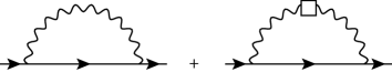
Figure 1: $\mathcal{O}(\alpha,\tilde{k})$ loop contributions to the fermion self-energy in the first perturbation scheme with $c^{\mu\nu}=0$. The single solid and wavy lines denote conventional Lorentz-symmetric electron and photon propagators, respectively. The box represents the Lorentz-violating $\tilde{k}$ insertion footnote-1 .

We begin our general discussion of the two-point function with a few general remarks about the choice of perturbation scheme. (An actual perturbative calculation of this function will have to wait until the next section.) To set up perturbation theory for calculating the radiative corrections to the two-point function we have to make a suitable choice of a zeroth-order system with known solutions, such that the remaining piece can be considered a small perturbation relative to this zeroth-order system. While usually one takes as the zeroth-order system the full quadratic part of the action, in the case at hand there are at least two reasonable choices one might consider.

In the first scheme, one defines as a basis the renormalized quadratic Lagrangian of the conventional Lorentz-symmetric case. All Lorentz-violating contributions to the Lagrangian are then taken as perturbations. One can, for example, use the minimal-subtraction scheme to define the counterterms (either Lorentz-symmetric or Lorentz-violating).

In the second scheme, one defines as a basis the full renormalized quadratic Lagrangian, including the Lorentz-violating part. The perturbations are then just the nonquadratic contributions to the Lagrangian. For the latter, it is convenient to join the corresponding Lorentz-symmetric and Lorentz-violating vertices in the same diagram. One can do this also for the counterterms.

A key difference between the two schemes concerns their kinematical features, which is best explained by an example. Consider the one-loop fermion self energy. In the conventional Lorentz-symmetric case, energy–momentum kinematics prohibits the internal photon and fermion lines from going on-shell simultaneously for physical incoming momenta. Let us next look at the leading-order Lorentz-violating generalization of this process in the above two schemes with focus on the special case with a photon $\tilde{k}$ coefficient only.

In the first scheme, this process involves the conventional diagram plus another version of the diagram with a $\tilde{k}$ insertion on the photon line represented by a box in Fig. 1. Both of these diagrams exhibit the same Lorentz-symmetric propagators and the same Lorentz-symmetric dispersion relation for external momenta. The energy–momentum kinematics is therefore unchanged relative to the conventional case. In particular, the internal photon and fermion propagators cannot go on-shell simultaneously for physical incoming momenta at this order in perturbation theory.

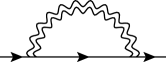
Figure 2: $\mathcal{O}(\alpha,\tilde{k})$ loop contributions to the fermion self energy in the second perturbation scheme with $c^{\mu\nu}=0$. The single solid line denotes the conventional Lorentz-symmetric electron propagator. The double wavy line represents the full Lorentz-violating photon propagator including all tree-level $\tilde{k}$ effects footnote-1 .

In the second scheme, there is a single diagram analogous to the conventional one, but with the usual photon propagator replaced by a Lorentz-violating propagator containing $\tilde{k}$, represented by a double photon line in Fig. 2. At this order, the dispersion relation of the incoming momentum remains Lorentz symmetric, but the $\tilde{k}$ propagator modifies the internal kinematics of the self-energy diagram. In particular, the internal photon and fermion lines can now go on-shell simultaneously for physical incoming momenta in certain regimes. This is evident from the well-established result AltCer that photons that are slowed down by certain values of $\tilde{k}$ lead to vacuum Cherenkov radiation at ultrahigh energies: a real free fermion can now emit a real photon. The nonzero cross section for this effect is then directly related to imaginary contributions to the fermion self-energy via the optical theorem. Note that imaginary contributions are absent in the first scheme.

Such Cherenkov instabilities are relatively rare: they do not occur for all Lorentz-violating coefficients and are in any case only present at ultrahigh energies in our model. They correspond exactly to the two-particle regime discussed in Ref. Potting:2011yj , where the Källén–Lehmann representation of the fermion two-point function was analyzed in the presence of a $c^{\mu\nu}$-type Lorentz-violating perturbation. As was shown there, for ultrahigh momenta the two-point function can pass from a stable one-particle regime into an unstable two-particle regime and provoke a Cherenkov-type decay. In the case at hand, the latter consists of the fermion plus a photon.

In this work, we are primarily interested in the properties of external states before such rare instabilities lead to their decay. We therefore omit imaginary contributions to the fermion self-energy. If needed, the physics of such instabilities may still be included subsequently, for example via cut diagrams using Cutkosky’s rules Cut . For the above purpose, which disregards instabilities, the two schemes become equivalent—a fact we have verified explicitly at one-loop order. For definiteness, we present our analysis in the second scheme. It has the advantage of being more economical, as the number of diagrams is considerably reduced. In particular, the diagrams in this scheme are in one-to-one correspondence with the diagrams in the Lorentz-symmetric case. Moreover, in the present context this scheme is free of momentum-routing ambiguities. Although the prescription for calculating the corresponding amplitude is more involved due to the Lorentz-violating coefficients, we have found that the full calculation is easier to carry out in the second scheme and is also less prone to error.

Explicitly, the second scheme implies that our model Lagrange density (13) is split into the following three pieces:

$$\mathcal{L}_{c\tilde{k}}=\mathcal{L}_{0}+\mathcal{L}_{1}+\mathcal{L}_{2}\,,$$ (14)

where

$$\mathcal{L}_{0} =\bar{\psi}\left[i\left(\gamma^{\mu}+c^{\mu\nu}\gamma_{\nu}\right)\partial_{\mu}-m\right]\psi$$

$$\>{}-\frac{1}{4}\left(\eta^{\mu\nu}+\tilde{k}^{\mu\nu}\right)\left(\eta^{\alpha\beta}+\tilde{k}^{\alpha\beta}\right)F_{\mu\alpha}F_{\nu\beta}$$

$$\>{}-\frac{1}{2\xi}\left(\partial_{\mu}A^{\mu}+\tilde{k}^{\mu\nu}\partial_{\mu}A_{\nu}\right)^{2}+\frac{m_{\gamma}^{2}}{2}A_{\mu}\left(\eta^{\mu\nu}+\tilde{k}^{\mu\nu}\right)A_{\nu}\,,$$ (15)

$$\mathcal{L}_{1} =\bar{\psi}\left[-e\left(\gamma^{\mu}+c^{\mu\nu}\gamma_{\nu}\right)A_{\mu}\right]\psi\,,$$ (16)

and

$$\mathcal{L}_{2} =\bar{\psi}\Bigl{[}\bigl{(}(Z_{\psi}-1)\eta^{\mu\nu}+Z_{\psi}(Z_{c}\,c)^{\mu\nu}-c^{\mu\nu}\bigr{)}i\gamma_{\nu}\left(\partial_{\mu}+ieA_{\mu}\right)$$

$$\qquad\qquad{}-(Z_{\psi}Z_{m}-1)m\Bigr{]}\psi$$

$$\quad{}-\frac{1}{4}\biggl{[}\left(Z_{A}-1\right)\eta^{\mu\nu}\eta^{\alpha\beta}+2\left(Z_{A}(Z_{k}\,\tilde{k})^{\mu\nu}-\tilde{k}^{\mu\nu}\right)\eta^{\alpha\beta}$$

$$\qquad\qquad{}+\Bigl{(}Z_{A}(Z_{k}\,\tilde{k})^{\mu\nu}(Z_{k}\,\tilde{k})^{\alpha\beta}-\tilde{k}^{\mu\nu}\tilde{k}^{\alpha\beta}\Bigr{)}\biggr{]}$$

$$\qquad\qquad{}\times\left(F_{\mu\alpha}F_{\nu\beta}+\frac{2}{\xi}\left(\partial_{\mu}A_{\nu}\right)\left(\partial_{\alpha}A_{\beta}\right)\right)$$

$$\quad{}+\frac{m_{\gamma}^{2}}{2}A_{\mu}\left[(Z_{A}-1)\eta^{\mu\nu}+Z_{A}(Z_{k}\,\tilde{k})^{\mu\nu}-\tilde{k}^{\mu\nu}\right]A_{\nu}\,.$$ (17)

The corresponding Feynman rules, which are collected in Appendix A, now facilitate an order-by-order calculation of our model’s two-point function

$$\Gamma^{(2)}(p)=\Gamma^{\mu}p_{\mu}-m-\Sigma(p^{\mu})\,.$$ (18)

Paralleling the conventional perturbative determination of this function, $\Sigma$ denotes the contribution of the one-particle irreducible Feynman diagrams. The summation procedure for these diagrams, which does not rely on Lorentz symmetry, closely parallels the conventional case and leads directly to Eq. (18).

Before proceeding with an actual one-loop calculation, it is instructive to determine the general structure of $\Sigma$. This structure is constrained by the requirement of coordinate independence, which dictates that $\Sigma$ can only depend on coordinate scalars formed by contractions of model parameters, external momenta, and gamma matrices. In particular, one can consider the propagator as an effective function of these contracted Lorentz scalars. This represents a direct generalization of the conventional case, where a single independent scalar, $\not{p}$, can be formed and the propagator can be treated as depending on $\not{p}$.

With these considerations in mind, we may decompose $\Sigma$ as

$$\Sigma=\Sigma_{\rm LI}(\not{p})+\Sigma_{\rm LV}(p^{2},c^{p}_{\gamma},\,\tilde{k}^{p}_{\gamma})+\delta\Sigma(p^{\mu},c^{\mu\nu},\tilde{k}^{\mu\nu})\,,$$ (19)

where we have defined $c^{p}_{\gamma}\equiv c^{\mu\nu}\gamma_{\mu}p_{\nu}$ and $\tilde{k}^{p}_{\gamma}\equiv\tilde{k}^{\mu\nu}\gamma_{\mu}p_{\nu}$. In this decomposition, $\Sigma_{\rm LI}(\not{p})$ denotes the Lorentz-symmetric contributions equivalent to the conventional diagrams; it can thus only be a function of $\not{p}$, as usual:

$$\Sigma_{\rm LI}(\not{p})=f_{0}(p^{2})m+f_{1}(p^{2})\,\not{p}\,,$$ (20)

where both $f_{0}(p^{2})$ and $f_{1}(p^{2})$ are understood to depend on the fine-structure constant $\alpha=e^{2}/4\pi$ and the square of the 4-momentum $p^{2}$. The remaining two terms involve deviations from Lorentz symmetry, so we will describe them in more detail.

The second term $\Sigma_{\rm LV}(p^{2},c^{p}_{\gamma},\tilde{k}^{p}_{\gamma})$ contains all those Lorentz-violating terms with a gamma-matrix structure that is already present in the fermion Lagrange density (i.e., a Lorentz-breaking symmetric traceless 2-tensor contracted with a gamma matrix and a single momentum factor). For example, $\Sigma_{\rm LV}$ includes the counterterms for $c^{\mu\nu}$ and $\tilde{k}^{\mu\nu}$ together with the corresponding (regulated) infinities they cancel to yield an ultraviolet finite expression:

$$\Sigma_{\rm LV}(p^{2},c^{p}_{\gamma},\tilde{k}^{p}_{\gamma})=f_{2}^{c}(p^{2})\,c^{p}_{\gamma}+f_{2}^{\tilde{k}}(p^{2})\,\tilde{k}^{p}_{\gamma}\,,$$ (21)

where $f_{2}^{c}(p^{2})$ and $f_{2}^{\tilde{k}}(p^{2})$ depend only on $\alpha$ and $p^{2}$ since we are working at leading order in Lorentz violation. Explicit expressions for $f_{2}^{c}(p^{2})$ and $f_{2}^{\tilde{k}}(p^{2})$ can in principle be determined within perturbation theory to any given order in $\alpha$. Below we will calculate $f_{2}^{c}(p^{2})$ and $f_{2}^{\tilde{k}}(p^{2})$ at one loop, i.e., at ${\cal O}(\alpha)$. Initially, $f_{2}^{c}(p^{2})$ and $f_{2}^{\tilde{k}}(p^{2})$ may also depend on an infrared regulator and an arbitrary mass scale introduced by the chosen ultraviolet regularization procedure. But a consistent treatment of infrared effects and the renormalization conditions should remove free parameters from $\Sigma_{\rm LV}(p^{2},c^{p}_{\gamma},\tilde{k}^{p}_{\gamma})$.

The remaining term $\delta\Sigma(p^{\mu},c^{\mu\nu},\tilde{k}^{\mu\nu})$ contains novel Lorentz-breaking structures that are not already present in the original Lagrange density (13). Like the second term, it must involve combinations of $p^{\mu}$ factors, $\gamma$ matrices, and—since we are working at linear order in Lorentz violation—a single $c^{\mu\nu}$ or $\tilde{k}^{\mu\nu}$ coefficient. Up to factors consisting of powers of $p^{2}$, a multitude of terms can be constructed that satisfy these requirements. They are

$$c^{\mu\nu}p_{\mu}p_{\nu}\,,\quad\not{p}\,c^{\mu\nu}p_{\mu}p_{\nu}\,,\quad\gamma^{5}c^{\mu\nu}p_{\mu}p_{\nu}\,,\quad\gamma^{5}\not{p}\,c^{\mu\nu}p_{\mu}p_{\nu}\,,$$

$$\gamma^{5}c^{\mu\nu}\gamma_{\mu}p_{\nu}\,,\quad\sigma^{\lambda\mu}c_{\lambda}{}^{\nu}p_{\mu}p_{\nu}\,,\quad\gamma^{5}\sigma^{\lambda\mu}c_{\lambda}{}^{\nu}p_{\mu}p_{\nu}\,,$$ (22)

as well as an additional seven terms with $c^{\mu\nu}$ replaced by $\tilde{k}^{\mu\nu}$ footnote0 .

The above list (III) can be constrained further by noting that electromagnetic interactions preserve C, P, and T. Quantum corrections linear in $c^{\mu\nu}$ and $\tilde{k}^{\mu\nu}$ must exhibit the same discrete symmetries as the original Lorentz-violating operators. This fact together with our scope set out earlier (i.e., omitting instabilities and thus non-Hermitian expressions) leaves only the first two terms in the list (III) and their $\tilde{k}^{\mu\nu}$ analogues footnote1 . For this reason, $\delta\Sigma(p^{\mu},c^{\mu\nu},\tilde{k}^{\mu\nu})$ can only depend on $c^{p}_{p}\equiv c^{\mu\nu}p_{\mu}p_{\nu}$ and $\tilde{k}^{p}_{p}\equiv\tilde{k}^{\mu\nu}p_{\mu}p_{\nu}$, and we may write

$$\delta\Sigma(p^{\mu},c^{p}_{p},\tilde{k}^{p}_{p}) =f_{3}^{c}(p^{2})\,\frac{c^{p}_{p}}{m}+f_{4}^{c}(p^{2})\,\frac{\not{p}c^{p}_{p}}{m^{2}}$$

$$\qquad{}+f_{3}^{\tilde{k}}(p^{2})\,\frac{\tilde{k}^{p}_{p}}{m}+f_{4}^{\tilde{k}}(p^{2})\,\frac{\not{p}\tilde{k}^{p}_{p}}{m^{2}}\,.$$ (23)

Here, we have introduced the dimensionless functions $f_{3}^{c}(p^{2})$, $f_{4}^{c}(p^{2})$, $f_{3}^{\tilde{k}}(p^{2})$, and $f_{4}^{\tilde{k}}(p^{2})$, which can in principle be calculated within perturbation theory to any given order in $\alpha$. These functions may initially still contain infrared regulators, which can presumably be removed by a soft-photon treatment. Disregarding the aforementioned possibility of high-energy non-Hermitian contributions, Eqs. (19), (20), (21), and (III) determine the full off-shell structure of the fermion two-point function in our $c\tilde{k}$ model (13) at all orders in $\alpha$ and at linear order in Lorentz violation.

Before deriving explicit expressions for the scalar functions appearing in the corrections (20), (21), and (III)—a task to which we will turn in Sec. IV—it is instructive to construct a general procedure for extracting the on-shell external-leg physics determined by the structure of these corrections. In general, external tree-level momentum-space Dirac spinors $w_{0}$ satisfy $P_{0}w_{0}=0$, where $P_{0}$ denotes the free Dirac operator of the theory (e.g., $P_{0}=\not{p}-m$ in the conventional case). The external states $w$ in the fully interacting theory must then satisfy an equation of the structure $(P_{0}+\delta P^{\prime})w=0$, where $\delta P^{\prime}$ is a small correction to $P_{0}$ PertCom . It is customary to rearrange this equation such that all terms proportional the matrix $\not{p}$ are removed from $\delta P^{\prime}$ ZCom . This yields $\mathcal{Z}_{R}^{-1}(P_{0}+\delta P)w=0$, where $\mathcal{Z}_{R}$ is some scalar function and $\delta P$ is properly adjusted relative to $\delta P^{\prime}$. For sufficiently small interactions, $\mathcal{Z}_{R}=1+\delta\mathcal{Z}_{R}$ should remain close to unity and is thus regular for on-shell momenta.

The expression $\bar{P}\equiv P_{0}+\delta P$ can be interpreted as the effective single-particle Dirac operator in the fully interacting theory, which governs the propagation of external states. Standard arguments now directly imply that the momentum-space Green function associated with $\bar{P}$ must have the structure $\mathcal{Z}_{R}\bar{P}{}^{-1}$. In addition to this one-particle pole, the two-point function may also contain additional off-shell effects and multiparticle physics, which can be included via a general term $R$ that remains regular in the vicinity of the pole:

$$\Gamma^{(2)}(p)^{-1}=\mathcal{Z}_{R}\bar{P}{}^{-1}-R\,.$$ (24)

This result is fully consistent with both the original Källen–Lehmann representation KallenLehmann and its recent generalization to Lorentz-violating theories Potting:2011yj .

The reasoning leading Eq. (24) leaves undetermined the detailed structures of $\mathcal{Z}_{R}$, $\delta P$, and $R$. However, perturbative expressions for these quantities can be determined. For example, one may compare an explicit loop-expansion result for $\Gamma^{(2)}(p)$ to the following form of Eq. (24),

$$\Gamma^{(2)}(p)=\mathcal{Z}_{R}^{-1}\bar{P}+\bar{P}\big{[}\mathcal{Z}_{R}^{-2}R(\openone-\mathcal{Z}_{R}^{-1}\bar{P}R)^{-1}\big{]}\bar{P}\,.$$ (25)

Note that up to this point, the above procedure, and in particular the result (25), are general and do not rely on Lorentz invariance. Symmetry considerations typically enter in the next step, when a general ansatz for $\delta P$ is posited and the free parameters contained in this ansatz are determined via comparison to the loop expression for $\Gamma^{(2)}(p)$.

As an example, let us briefly review the essence of the conventional QED case. A perturbative evaluation of the two-point function yields

$$\Gamma^{(2)}_{\rm LI}=A(p^{2})\not{p}+M(p^{2})\openone=A(\not{p}\not{p})\not{p}-M(\not{p}\not{p})\openone\,,$$ (26)

with explicit expressions for $A(p^{2})$ and $M(p^{2})$ that depend on the order in pertubation theory LIcomment . One then considers the ansatz

$$\bar{P}=\not{p}-m_{\rm ph}$$ (27)

for the dispersion relation LIcomment , where $m_{\rm ph}$ is a free parameter to be determined. Note that this is the most general form of $\bar{P}$ that represents a correction to the tree-level case and exhibits the canonical normalization of $\not{p}$, as discussed above.

With this ansatz, we may rewrite $\Gamma^{(2)}_{\rm LI}$ in Eq. (26) as a function of $\bar{P}$ rather than $\not{p}$:

$$\Gamma^{(2)}_{\rm LI}(\bar{P}) = A(\bar{P}{}^{2}+2m_{\rm ph}\bar{P}+m_{\rm ph}^{2})\bar{P}$$ (28)

$${}+m_{\rm ph}A(\bar{P}{}^{2}+2m_{\rm ph}\bar{P}+m_{\rm ph}^{2})\openone$$

$${}-M(\bar{P}{}^{2}+2m_{\rm ph}\bar{P}+m_{\rm ph}^{2})\openone\,.$$

The on-shell condition $\Gamma^{(2)}_{\rm LI}(\bar{P}=0)=0$ yields an implicit relation for $m_{\rm ph}$

$$0=m_{\rm ph}A(m_{\rm ph}^{2})-M(m_{\rm ph}^{2})\,,$$ (29)

which can be employed to determine the physical mass.

Expanding $\Gamma^{(2)}_{\rm LI}(\bar{P})$ around the pole $\bar{P}=0$ gives

$$\Gamma^{(2)}_{\rm LI}(\bar{P})=\Gamma^{(2)}_{\rm LI}{}^{\prime}(0)\,\bar{P}+\bar{P}\Big{[}\sum_{n=2}^{\infty}\frac{\Gamma^{(2)}_{\rm LI}{}^{(n)}(0)}{n!}\,\bar{P}{}^{n-2}\Big{]}\bar{P}\,,$$ (30)

where the zeroth-order term in the expansion vanishes by virtue of Eq. (29). Comparison with the general result (25) then establishes

$$\mathcal{Z}_{R}^{-1} = \Gamma^{(2)}_{\rm LI}{}^{\prime}(0)$$ (31)

$$= 2m_{\rm ph}^{2}\big{[}A^{\prime}(m_{\rm ph}^{2})-M^{\prime}(m_{\rm ph}^{2})\big{]}+A(m_{\rm ph}^{2})\,.$$

It is now apparent that Eqs. (29) and (31) completely fix the expression for pole. Note that in the above Lorentz-symmetric situation, the only nontrivial Dirac-matrix structure is $\not{p}$, so that no matrix-ordering issues arise.

In the present Lorentz-violating case, we may follow a similar line of reasoning, albeit with generalized versions of the above Eqs. (26) and (27). Our previous result for the general structure of our model’s two-point function, which is summarized in Eqs. (18)–(III), may be recast into the following form:

$$\Gamma^{(2)}=A(p^{2}\!,c^{p}_{p},\tilde{k}^{p}_{p})\not{p}+C(p^{2})c^{p}_{\gamma}+K(p^{2})\tilde{k}^{p}_{\gamma}-M(p^{2}\!,c^{p}_{p},\tilde{k}^{p}_{p})\,.$$ (32)

Using our previous definitions, we have at leading order in Lorentz violation:

$$A\! = \!1-f_{1}(p^{2})-f_{4}^{c}(p^{2})\frac{c^{p}_{p}}{m^{2}}-f_{4}^{\tilde{k}}(p^{2})\frac{\tilde{k}^{p}_{p}}{m^{2}}\,,$$

$$C\! = \!1-f_{2}^{c}(p^{2})\,,$$

$$K\! = \!-f_{2}^{\tilde{k}}(p^{2})\,,$$

$$M\! = \!m\big{[}1+f_{0}(p^{2})\big{]}+f_{3}^{c}(p^{2})\frac{c^{p}_{p}}{m}+f_{3}^{\tilde{k}}(p^{2})\frac{\tilde{k}^{p}_{p}}{m}\,.$$ (33)

Note that the presence of the Lorentz-breaking parameters $c^{\mu\nu}$ and $\tilde{k}^{\mu\nu}$ leads to two new features relative to the Lorentz-symmetric expression (26). First, the coefficient functions $A$ and $M$ can now also depend $c^{p}_{p}$ and $\tilde{k}^{p}_{p}$; these are the only coordinate scalars in addition to $p^{2}$ that can be formed at leading order in Lorentz violation. Second, two additional gamma-matrix structures, namely $c^{p}_{\gamma}$ and $\tilde{k}^{p}_{\gamma}$, and their respective coefficient functions $C(p^{2},c^{p}_{p},\tilde{k}^{p}_{p})$ and $K(p^{2},c^{p}_{p},\tilde{k}^{p}_{p})$ can now be formed. As for the Lorentz-invariant case, the detailed expressions for $A$, $M$, $C$, and $K$ depend on the order in $\alpha$ under consideration.

Next, we need the generalization of the ansatz (27). Employing the results of Ref. Potting:2011yj at leading order in $c^{\mu\nu}$ and $\tilde{k}^{\mu\nu}$, we find the most general form for the pole to be

$$\bar{P}=\not{p}-\bar{m}+\bar{x}c^{p}_{\gamma}+\bar{y}\tilde{k}^{p}_{\gamma}\,.$$ (34)

Here, the coefficient functions $\bar{m}$, $\bar{x}$, and $\bar{y}$ do not depend on $p^{2}$. This is intuitively reasonable, since on-shell we may replace $p^{2}\to m_{\rm ph}^{2}+{\cal O}(c^{p}_{p},\tilde{k}^{p}_{p})$. In any case, this follows rigorously from the results in Ref. Potting:2011yj . This means we can take $\bar{x}$ and $\bar{y}$ to be free constants to be determined later. Similarly,

$$\bar{m}=m_{\rm ph}+m_{c}c^{p}_{p}+m_{k}\tilde{k}^{p}_{p}\,,$$ (35)

with $m_{\rm ph}$, $m_{c}$, and $m_{k}$ momentum-independent parameters to be determined below. Note that as opposed to the usual Lorentz-symmetric ansatz (27), which contains the single free quantity $m_{\rm ph}$, the corresponding ansatz for our Lorentz-violating model is parametrized by five free coefficients $\bar{x}$, $\bar{y}$, $m_{\rm ph}$, $m_{c}$, and $m_{k}$.

Paralleling the usual Lorentz-invariant reasoning, we now use our ansatz (34) to replace $\not{p}$ and $p^{2}=\not{p}\not{p}$ by $\bar{P}$ in the expression for the two-point function (32). To this end, it is useful to write

$$p^{2}=\not{p}\not{p}=\bar{P}\bar{P}+2\bar{m}\bar{P}+\bar{\beta}\,,$$ (36)

where at leading order in Lorentz violation

$$\bar{\beta}=\bar{m}^{2}-2\bar{x}c^{p}_{p}-2\bar{y}\tilde{k}^{p}_{p}\,.$$ (37)

This produces the Lorentz-breaking analogue of Eq. (28):

$$\Gamma^{(2)}(\bar{P}) = A(\bar{P}{}^{2}+2\bar{m}\bar{P}+\bar{\beta},c^{p}_{p},\tilde{k}^{p}_{p})\bar{P}$$ (38)

$${}+\bar{m}A(\bar{P}{}^{2}+2\bar{m}\bar{P}+\bar{\beta},c^{p}_{p},\tilde{k}^{p}_{p})\openone$$

$${}-M(\bar{P}{}^{2}+2\bar{m}\bar{P}+\bar{\beta},c^{p}_{p},\tilde{k}^{p}_{p})\openone$$

$${}+C(\bar{P}{}^{2}+2\bar{m}\bar{P}+\bar{\beta})c^{p}_{\gamma}$$

$${}-\bar{x}A(\bar{P}{}^{2}+2\bar{m}\bar{P}+\bar{\beta},c^{p}_{p},\tilde{k}^{p}_{p})c^{p}_{\gamma}$$

$${}+K(\bar{P}{}^{2}+2\bar{m}\bar{P}+\bar{\beta})\tilde{k}^{p}_{\gamma}$$

$${}-\bar{y}A(\bar{P}{}^{2}+2\bar{m}\bar{P}+\bar{\beta},c^{p}_{p},\tilde{k}^{p}_{p})\tilde{k}^{p}_{\gamma}\,.$$

Although some higher-order terms in Lorentz violation appear in this expression for notational convenience, Eq. (38) holds at linear order in $c^{\mu\nu}$ and $\tilde{k}^{\mu\nu}$.

We proceed by evaluating $\Gamma^{(2)}(\bar{P})$ at $\bar{P}=0$. As $\bar{P}$ is our ansatz for the pole, we must have $\Gamma^{(2)}(\bar{P}=0)=0$. This yields

$$0 = \big{[}C(\bar{\beta},c^{p}_{p},\tilde{k}^{p}_{p})-\bar{x}A(\bar{\beta},c^{p}_{p},\tilde{k}^{p}_{p})\big{]}c^{p}_{\gamma}$$ (39)

$${}+\big{[}K(\bar{\beta},c^{p}_{p},\tilde{k}^{p}_{p})-\bar{y}A(\bar{\beta},c^{p}_{p},\tilde{k}^{p}_{p})\big{]}\tilde{k}^{p}_{\gamma}$$

$${}+\big{[}\bar{m}A(\bar{\beta},c^{p}_{p},\tilde{k}^{p}_{p})-M(\bar{\beta},c^{p}_{p},\tilde{k}^{p}_{p})\big{]}\openone\,.$$

Since $c^{\mu\nu}$ and $\tilde{k}^{\mu\nu}$ are in general not proportional PropComment , we take $c^{p}_{\gamma}$ and $\tilde{k}^{p}_{\gamma}$ to be linearly independent, so that each square bracket in Eq. (39) must vanish separately. The two relations resulting from the first two brackets are needed at zeroth order in Lorentz violation; they can be cast into the following form:

$$\bar{x} = \frac{C(m_{\rm ph}^{2})}{A(m_{\rm ph}^{2})}\,,$$ (40)

$$\bar{y} = \frac{K(m_{\rm ph}^{2})}{A(m_{\rm ph}^{2})}\,.$$ (41)

Notice that $A(m_{\rm ph}^{2},0,0)=A(m_{\rm ph}^{2})$ is the conventional coefficient function for the Lorentz-invariant case. In a similar manner, we have defined $C(m_{\rm ph}^{2})\equiv C(m_{\rm ph}^{2},0,0)$ and $K(m_{\rm ph}^{2})\equiv K(m_{\rm ph}^{2},0,0)$. The relation arising from the third square bracket in Eq. (39) is needed at first order in Lorentz violation, so we may expand in $c^{p}_{p}$ and $\tilde{k}^{p}_{p}$ as follows:

$${}0\! = \!\bar{m}A(\bar{\beta},c^{p}_{p},\tilde{k}^{p}_{p})-M(\bar{\beta},c^{p}_{p},\tilde{k}^{p}_{p})$$ (42)

$$= \!\big{[}m_{\rm ph}A(m_{\rm ph}^{2})-M(m_{\rm ph}^{2})\big{]}$$

$$\!{}+\partial_{c^{p}_{p}}\big{[}\bar{m}A(\bar{\beta},c^{p}_{p},\tilde{k}^{p}_{p})-M(\bar{\beta},c^{p}_{p},\tilde{k}^{p}_{p})\big{]}_{c^{p}_{p},\tilde{k}^{p}_{p}=0}\;c^{p}_{p}$$

$$\!{}+\partial_{\tilde{k}^{p}_{p}}\big{[}\bar{m}A(\bar{\beta},c^{p}_{p},\tilde{k}^{p}_{p})-M(\bar{\beta},c^{p}_{p},\tilde{k}^{p}_{p})\big{]}_{c^{p}_{p},\tilde{k}^{p}_{p}=0}\;\tilde{k}^{p}_{p}\,.$$

We note that $M(m_{\rm ph}^{2},0,0)=M(m_{\rm ph}^{2})$ is the usual Lorentz-symmetric coefficient function. As we have taken $c^{\mu\nu}$ and $\tilde{k}^{\mu\nu}$ to be linearly independent, each square bracket in Eq. (42) must be equal to zero individually, which yields three algebraic equations:

$$0 = m_{\rm ph}A(m_{\rm ph}^{2})-M(m_{\rm ph}^{2})\,,$$ (43)

$$0 = \partial_{c^{p}_{p}}\big{[}\bar{m}A(\bar{\beta},c^{p}_{p},\tilde{k}^{p}_{p})-M(\bar{\beta},c^{p}_{p},\tilde{k}^{p}_{p})\big{]}_{c^{p}_{p},\tilde{k}^{p}_{p}=0}\,,$$ (44)

$$0 = \partial_{\tilde{k}^{p}_{p}}\big{[}\bar{m}A(\bar{\beta},c^{p}_{p},\tilde{k}^{p}_{p})-M(\bar{\beta},c^{p}_{p},\tilde{k}^{p}_{p})\big{]}_{c^{p}_{p},\tilde{k}^{p}_{p}=0}\,.$$ (45)

The five relations (40), (41), (43), (44), and (45) determine the five parameters $m_{\rm ph}$, $\bar{x}$, $\bar{y}$, $m_{c}$, and $m_{k}$ in our ansatz for the pole (34) in terms of the functions $A$, $C$, $K$, and $M$, which are calculable in perturbation theory. It follows that the expression for $\bar{P}$ is now completely fixed. These five relations constitute a direct generalization of Eq. (29) valid in the usual Lorentz-symmetric context. In particular, Eq. (29) governing the Lorentz-invariant case is identical to Eq. (43) in the Lorentz-breaking situation. We remark that as a consequence the value of the physical mass $m_{\rm ph}$—which we interpret as the momentum-independent piece of the coefficient of $\overline{\psi}\psi$—remains unaffected by Lorentz violation.

The remaining task is to extract the field-strength renormalization ${\cal Z}_{R}$. To this end, we may again proceed in a manner similar to the Lorentz-invariant situation and expand the perturbation-theory two-point function $\Gamma^{(2)}(\bar{P})$ around $\bar{P}=0$. As opposed to the conventional case, where only a single nontrivial matrix given by $\not{p}$ appears, the present Lorentz-violating situation involves the three matrices $\not{p}$, $c^{p}_{\gamma}$, and $\tilde{k}^{p}_{\gamma}$, which are in general noncommuting. For this reason, the expansion of $\Gamma^{(2)}(\bar{P})$, which we have relegated to Appendix B, requires special care to avoid matrix-ordering ambiguities. We find

$${\cal Z}_{R}^{-1}\! = \!A(\bar{\beta},c^{p}_{p},\tilde{k}^{p}_{p})+2\bar{m}\big{[}\bar{m}A^{\prime}(\bar{\beta},c^{p}_{p},\tilde{k}^{p}_{p})-M^{\prime}(\bar{\beta},c^{p}_{p},\tilde{k}^{p}_{p})\big{]}$$ (46)

$${}\!+2\big{[}C^{\prime}(m_{\rm ph}^{2})-\bar{x}A^{\prime}(m_{\rm ph}^{2})\big{]}c^{p}_{p}$$

$${}\!+2\big{[}K^{\prime}(m_{\rm ph}^{2})-\bar{y}A^{\prime}(m_{\rm ph}^{2})\big{]}\tilde{k}^{p}_{p}\,,$$

where a prime denotes the derivative with respect to the first argument.

IV One-loop calculation of the modified propagator

An interesting question concerns the determination of the functions $f_{0}(p^{2})$, $f_{1}(p^{2})$, $f_{2}^{c}(p^{2})$, $f_{2}^{\tilde{k}}(p^{2})$, $f_{3}^{c}(p^{2})$, $f_{4}^{c}(p^{2})$, $f_{3}^{\tilde{k}}(p^{2})$, and $f_{4}^{\tilde{k}}(p^{2})$ perturbatively at leading order in the fine-structure constant $\alpha$. To this end, we will adopt the perturbative scheme based on the expressions (14)–(17), in which the propagators are built from the full quadratic Lagrange density, including the Lorentz-violating parts. The corresponding Feynman rules are presented in Appendix A, and the only loop diagram involved in the fermion self-energy is shown in Fig. 3.

This diagram together with the corresponding counterterm contributions contains the conventional Lorentz-symmetric $\mathcal{O}(\alpha)$ results

$$f_{0}(p^{2}) =\frac{\alpha}{\pi}\left[-\frac{1}{2}-\gamma_{E}-\int_{0}^{1}dy\,\ln\left(\frac{\Delta}{4\pi\mu^{2}}\right)\right]\,,$$ (47)

$$f_{1}(p^{2}) =\frac{\alpha}{4\pi}\left[1+\gamma_{E}+2\int_{0}^{1}dy\,(1-y)\ln\left(\frac{\Delta}{4\pi\mu^{2}}\right)\right]$$ (48)

Here,

$$\Delta=-y(1-y)p^{2}+y(m^{2}-m_{\gamma}^{2})+m_{\gamma}^{2},$$ (49)

$\gamma_{E}=0.57721\ldots$ denotes the Euler–Mascheroni constant, $m_{\gamma}$ represents a fictitious photon mass introduced as an infrared regulator, and the arbitrary mass scale $\mu$ is a remnant from dimensional regularization. The integrations over $y$ can be performed requiring $p^{2}$ to be close to the conventional mass shell: $(m-m_{\gamma})^{2}<p^{2}<(m+m_{\gamma})^{2}$. They yield the infrared-finite limits on the (conventional) mass shell,

$$f_{0}(m^{2}) = \frac{\alpha}{\pi}\left[\frac{3}{2}-\gamma_{E}-\ln\left(\frac{m^{2}}{4\pi\mu^{2}}\right)\right]\,,$$ (50)

$$f_{1}(m^{2}) = \frac{\alpha}{\pi}\left[-\frac{1}{2}+\frac{\gamma_{E}}{4}+\frac{1}{4}\ln\left(\frac{m^{2}}{4\pi\mu^{2}}\right)\right].$$ (51)

For the on-shell values of their first and second derivatives we find at leading order in $m_{\gamma}$,

$$f_{0}^{\prime}(m^{2}) = \frac{\alpha}{\pi m^{2}}\left[\ln\left(\frac{m}{m_{\gamma}}\right)-1\right],$$ (52)

$$f_{0}^{\prime\prime}(m^{2}) = \frac{\alpha}{4\pi m^{4}}\left[\pi\,\frac{m}{m_{\gamma}}-8\ln\left(\frac{m}{m_{\gamma}}\right)+6\right],$$ (53)

$$f_{1}^{\prime}(m^{2}) = \frac{\alpha}{\pi m^{2}}\left[-\frac{1}{2}\ln\left(\frac{m}{m_{\gamma}}\right)+\frac{3}{4}\right],$$ (54)

$$f_{1}^{\prime\prime}(m^{2}) = \frac{\alpha}{8\pi m^{4}}\left[-\pi\,\frac{m}{m_{\gamma}}+12\ln\left(\frac{m}{m_{\gamma}}\right)-14\right].\quad$$ (55)

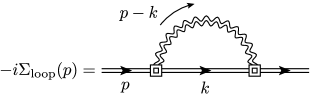
Figure 3: One-loop Feynman diagram for the determination of the fermion self-energy at ${\cal O}(\alpha)$. The complete $\Sigma$ at this order also contains counterterm insertion diagrams that have not been included above.

An explicit calculation also yields ultraviolet-finite expressions for the remaining, Lorentz-violating contributions to $\Sigma$. For the functions $f_{i}^{c}(p^{2})$, we obtain

$${}f_{2}^{c}(p^{2}) = \frac{\alpha}{2\pi}\biggl{[}\frac{1}{6}-\frac{5\gamma_{E}}{6}$$ (56)

$$\>{}-\int_{0}^{1}dy(1-y)(1+2y)\ln\left(\frac{\Delta}{4\pi\mu^{2}}\right)\biggl{]},$$

$${}f_{3}^{c}(p^{2}) = \frac{2\alpha m^{2}}{\pi}\int_{0}^{1}dy\frac{y(1-y)^{2}}{\Delta}\,,$$ (57)

$${}f_{4}^{c}(p^{2}) = -\frac{\alpha m^{2}}{\pi}\int_{0}^{1}dy\frac{y(1-y)^{3}}{\Delta}\,.$$ (58)

While $f_{2}^{c}(p^{2})$ is infrared finite, this is not the case for $f_{3}^{c}(p^{2})$ and $f_{4}^{c}(p^{2})$: the latter both diverge on the conventional mass shell $p^{2}=m^{2}$ when the limit $m_{\gamma}\to 0$ is taken:

$$f_{2}^{c}(m^{2}) = \frac{\alpha}{\pi}\left[\frac{10}{9}-\frac{5\gamma_{E}}{12}-\frac{5}{12}\ln\left(\frac{m^{2}}{4\pi\mu^{2}}\right)\right],$$ (59)

$$f_{3}^{c}(m^{2}) = \frac{\alpha}{\pi}\left[2\ln\left(\frac{m}{m_{\gamma}}\right)-3\right],$$ (60)

$$f_{4}^{c}(m^{2}) = \frac{\alpha}{\pi}\left[-\ln\left(\frac{m}{m_{\gamma}}\right)+\frac{11}{6}\right].$$ (61)

Below, we will also need the derivatives of these functions at their on-shell value $p^{2}=m^{2}$. To this effect, we use that

$$\frac{d}{dp^{2}}\ln\Delta=-\frac{y(1-y)}{\Delta}\,,\qquad\frac{d}{dp^{2}}\frac{1}{\Delta}=\frac{y(1-y)}{\Delta^{2}}\,.$$ (62)

Applying these relations to Eqs. (56)–(58), and evaluating the integrals on the conventional mass shell yields the following results:

$$f_{2}^{c}{}^{\prime}(m^{2}) = \frac{\alpha}{2\pi m^{2}}\left[\ln\left(\frac{m}{m_{\gamma}}\right)-\frac{5}{6}\right],$$ (63)

$$f^{c}_{3}{}^{\prime}(m^{2}) = \frac{\alpha}{\pi m^{2}}\left[\frac{\pi}{2}\frac{m}{m_{\gamma}}-6\ln\left(\frac{m}{m_{\gamma}}\right)+7\right],$$ (64)

$$f_{4}^{c}{}^{\prime}(m^{2}) = \frac{\alpha}{\pi m^{2}}\left[-\frac{\pi}{4}\frac{m}{m_{\gamma}}+4\ln\left(\frac{m}{m_{\gamma}}\right)-\frac{35}{6}\right].$$ (65)

Note that $f_{3}^{c}{}^{\prime}(p^{2})$ and $f_{4}^{c}{}^{\prime}(p^{2})$ have linear, rather than logarithmic, infrared divergences.

For the coefficients $f_{i}^{\tilde{k}}(p^{2})$ one finds

$$f_{2}^{\tilde{k}}(p^{2}) = \frac{\alpha}{\pi}\Bigl{[}\frac{1}{12}+\frac{\gamma_{E}}{3}$$ (66)

$${}+\frac{1}{2}\int_{0}^{1}dy(1-y^{2})\ln\left(\frac{\Delta}{4\pi\mu^{2}}\Bigr{)}\right]\,,$$

$$f_{3}^{\tilde{k}}(p^{2}) = \frac{\alpha m^{2}}{\pi}\int_{0}^{1}dy\frac{y^{2}(1-y)}{\Delta}\,,$$ (67)

$$f_{4}^{\tilde{k}}(p^{2}) = -\frac{\alpha m^{2}}{2\pi}\int_{0}^{1}dy\frac{y^{2}(1-y)^{2}}{\Delta}\,.$$ (68)

All three coefficients $f_{i}^{\tilde{k}}(p^{2})$ are infrared finite on the conventional mass shell:

$$f_{2}^{\tilde{k}}(m^{2}) = \frac{\alpha}{\pi}\left[-\frac{29}{36}+\frac{\gamma_{E}}{3}+\frac{1}{3}\ln\left(\frac{m^{2}}{4\pi\mu^{2}}\right)\right]\,,$$ (69)

$$f_{3}^{\tilde{k}}(m^{2}) = \frac{\alpha}{2\pi}\,,$$ (70)

$$f_{4}^{\tilde{k}}(m^{2}) = -\frac{\alpha}{6\pi}\,.$$ (71)

Applying the relations (62) to Eqs. (66)–(68) and evaluating the integrals at $p^{2}=m^{2}$, one finds the infrared-divergent expressions

$$f_{2}^{\tilde{k}}{}^{\prime}(m^{2}) = \frac{\alpha}{\pi m^{2}}\left[-\frac{1}{2}\ln\left(\frac{m}{m_{\gamma}}\right)+\frac{7}{12}\right],$$ (72)

$$f_{3}^{\tilde{k}}{}^{\prime}(m^{2}) = \frac{\alpha}{\pi m^{2}}\left[\ln\left(\frac{m}{m_{\gamma}}\right)-2\right],$$ (73)

$$f_{4}^{\tilde{k}}{}^{\prime}(m^{2}) = \frac{\alpha}{\pi m^{2}}\left[-\frac{1}{2}\ln\left(\frac{m}{m_{\gamma}}\right)+\frac{7}{6}\right].$$ (74)

Let us now see how the above one-loop calculation and the general formalism developed in Sec. III can be used to determine explicit ${\cal O}(\alpha)$ expressions for $\bar{P}$ and ${\cal Z}_{R}$ in terms of our model’s coefficients. This section’s results together with the definitions (III) yield the one-loop approximation of Eq. (43), which can be solved at ${\cal O}(\alpha)$:

$$m_{\rm ph}\! = \!m\big{[}1+f_{0}(m^{2})+f_{1}(m^{2})\big{]}$$ (75)

$$= \!m+\frac{\alpha}{\pi}\left[1-\frac{3\gamma_{E}}{4}-\frac{3}{4}\ln\left(\frac{m^{2}}{4\pi\mu^{2}}\right)\right]m\,.$$

With this result, the parameters $\bar{x}$ and $\bar{y}$ directly follow from Eqs. (40) and (41) at one-loop order:

$$\bar{x} = 1+f_{1}(m^{2})-f_{2}^{c}(m^{2})$$ (76)

$$= 1+2\frac{\alpha}{\pi}\left[-\frac{29}{36}+\frac{\gamma_{E}}{3}+\frac{1}{3}\ln\left(\frac{m^{2}}{4\pi\mu^{2}}\right)\right],$$

$$\bar{y} = -f_{2}^{\tilde{k}}(m^{2})$$ (77)

$$= -\frac{\alpha}{\pi}\left[-\frac{29}{36}+\frac{\gamma_{E}}{3}+\frac{1}{3}\ln\left(\frac{m^{2}}{4\pi\mu^{2}}\right)\right].$$

We continue with the determination of $m_{c}$ and $m_{k}$ from Eqs. (44) and (45), respectively. To this end, notice that $\bar{\beta}=m^{2}-2c^{p}_{p}+\mathcal{O}(\alpha)$, which gives

$$\big{[}\partial_{c^{p}_{p}}f_{0}(\bar{\beta})\big{]}_{c^{p}_{p},\tilde{k}^{p}_{p}=0}=-2f^{\prime}_{0}(m^{2})+\mathcal{O}(\alpha^{2})\,,$$ (78)

with an analogous result for the function $f_{1}$. We then find at leading order in $\alpha$:

$$m_{c}\! = \!-2m\big{[}f_{0}^{\prime}(m^{2})+f_{1}^{\prime}(m^{2})\big{]}+\frac{1}{m}\big{[}f_{3}^{c}(m^{2})+f_{4}^{c}(m^{2})\big{]}$$ (79)

$$= \!-\frac{2\alpha}{3\pi m}\,,$$

$$m_{k}\! = \!\frac{1}{m}\big{[}f_{3}^{\tilde{k}}(m^{2})+f_{4}^{\tilde{k}}(m^{2})\big{]}$$ (80)

$$= \!\frac{\alpha}{3\pi m}\,.$$

The above results together with the general formula (46) allow us to give the following explicit form of the wave-function renormalization at one-loop order:

$$\mathcal{Z}_{R}^{-1} =1-f_{1}(m^{2})-2m^{2}\Big{[}f_{0}^{\prime}(m^{2})+f_{1}^{\prime}(m^{2})\Big{]}$$

$$\quad{}+2c^{p}_{p}\bigg{[}2f_{1}^{\prime}(m^{2})+2m^{2}f_{0}^{\prime\prime}(m^{2})+2m^{2}f_{1}^{\prime\prime}(m^{2})$$

$$\quad{}-f_{2}^{c}{}^{\prime}(m^{2})-f_{3}^{c}{}^{\prime}(m^{2})-f_{4}^{c}{}^{\prime}(m^{2})-\frac{f_{4}^{c}(m^{2})}{2m^{2}}\bigg{]}$$

$$\quad{}-2\tilde{k}^{p}_{p}\bigg{[}f_{2}^{\tilde{k}}{}^{\prime}(m^{2})+f_{3}^{\tilde{k}}{}^{\prime}(m^{2})+f_{4}^{\tilde{k}}{}^{\prime}(m^{2})+\frac{f_{4}^{\tilde{k}}(m^{2})}{2m^{2}}\bigg{]}$$

$$=1-\frac{\alpha}{\pi}\left[\ln\left(\frac{m}{m_{\gamma}}\right)-1+\frac{\gamma_{E}}{4}+\frac{1}{4}\ln\left(\frac{m^{2}}{4\pi\mu^{2}}\right)\right]$$

$$\quad{}-\frac{2\alpha}{3\pi m^{2}}(2\,c^{p}_{p}-\tilde{k}^{p}_{p})\,.$$ (81)

The Lorentz-symmetric piece of $\mathcal{Z}_{R}$ is identical to the conventional one-loop wave-function renormalization constant for the fermion in QED. In particular, it exhibits the usual logarithmic infrared divergence. On the other hand, the linear and logarithmic infrared divergences that are present in the various individual $f$ coefficient functions that multiply $c^{p}_{p}$ and $\tilde{k}^{p}_{p}$ in the intermediate step are absent in the final expression of Eq. (81). As is well known, the Lorentz-symmetric infrared divergences cancel in scattering cross sections when the contributions of soft-photon emission from the corresponding external legs are taken into account. In Sec. VI, we will verify that these soft-photon contributions do not introduce additional infrared divergences proportional to $c^{p}_{p}$ or $\tilde{k}^{p}_{p}$, so that physical observables remain infrared finite. We also note that the Lorentz-violating radiative corrections indeed appear in the combination $(2c^{\mu\nu}-\tilde{k}^{\mu\nu})$, as anticipated in Sec. II.

A novel feature relative to the Lorentz-invariant situation is the momentum dependence of ${\cal Z}_{R}$. We do not see any conceptual issues arising from this feature in the momentum range that is of phenomenological interest. However, bounds on ${\cal Z}_{R}$ obtained nonperturbatively on physical grounds may perhaps be used together with Eq. (81) to investigate the validity of perturbation theory at ultrahigh momenta.

We are now also in a position to determine explicit expressions for physically measurable model parameters. These can be identified via inspection of Eqs. (34) and (35). For example, it is apparent that $m_{\rm ph}$, which is given explicitly at order $\alpha$ in Eq. (75), is the measurable mass parameter governing the propagation of asymptotic states. The terms $\bar{x}c^{p}_{\gamma}$ and $\bar{y}k^{p}_{\gamma}$ in the inverse propagator (34) cannot individually be resolved in an experiment. Instead, their sum is interpreted to determine the physical $c$ coefficient denoted by $c_{\rm ph}^{\mu\nu}$,

$$c_{\rm ph}^{\mu\nu} =\bar{x}c^{\mu\nu}+\bar{y}\tilde{k}^{\mu\nu}$$

$$=c^{\mu\nu}-\frac{\alpha}{3\pi}\left[\frac{29}{12}-\gamma_{E}-\ln\left(\frac{m^{2}}{4\pi\mu^{2}}\right)\right](2c^{\mu\nu}-\tilde{k}^{\mu\nu})\,,$$ (82)

where the last equality is based on our above one-loop results. Note again that the radiative corrections depend on $(2c^{\mu\nu}-\tilde{k}^{\mu\nu})$ in line with our discussion in Sec. II. Note also that $c_{\rm ph}^{\mu\nu}$ is free of infrared divergences. We finally remark that unlike $c_{\rm ph}^{\mu\nu}$, both $c^{\mu\nu}$ and the scale $\mu$ are unphysical renormalization-scheme-dependent quantities. In particular, the running of $c^{\mu\nu}$ with $\mu$ Kostelecky:2001jc cancels the explicit appearances of $\mu$ in Eq. (82), so that $c_{\rm ph}^{\mu\nu}$ is independent of $\mu$. This situation is completely analogous to the conventional relation (75) expressing the constant $m_{\rm ph}$ in terms of $\mu$ and the running mass $m$.

Relative to the tree-level expression

$$\bar{P}_{\scriptsize\rm tree}(p)=\not{p}+c^{p}_{\gamma}-m\,,$$ (83)

the full Dirac operator (34) not only contains the above radiative corrections to the existing $m$ and $c^{\mu\nu}$ pieces, but it also displays the new structures $m_{c}c^{p}_{p}$ and $m_{k}k^{p}_{p}$, which possess more than a single power of momentum. Our results (79) and (80) show that the coefficients $m_{c}$ and $m_{k}$ are nonzero. At one-loop order, the asymptotic Dirac operator $\bar{P}_{1}$ can therefore be written in the form k_comment

$$\bar{P}_{1}=\not{p}+(c_{\scriptsize\rm ph})^{p}_{\gamma}-m_{\scriptsize\rm ph}+\frac{\alpha}{3\pi m}\big{[}2(c_{\scriptsize\rm ph})^{p}_{p}-(\tilde{k}_{\scriptsize\rm ph})^{p}_{p}\big{]}\,.$$ (84)

In accordance with the general expectation discussed in Sec. II, the new structures—shown as the last term in Eq. (84)—enter in the combination $(2c^{\mu\nu}-\tilde{k}^{\mu\nu})$. The fact that in addition to shifts in existing model parameters, asymptotic states in Lorentz-violating field theories also acquire novel higher-derivative $\mu$-independent structures represents a key finding of our work. We remark that this result is fully compatible with the general form of the one-particle fermion pole of the Källén–Lehmann representation derived in Ref. Potting:2011yj .

With the asymptotic Dirac operator (34) and its one-loop approximation (84) at hand, we may determine various properties of the external fermion states. For example, the corresponding two forms of the dispersion relation are given by

$$0 =p^{2}+2\bar{x}c^{p}_{p}+2\bar{y}\tilde{k}^{p}_{p}-m_{\rm ph}^{2}-2m_{\rm ph}(m_{c}c^{p}_{p}+m_{k}k^{p}_{p})$$

$$=p^{2}+2(c_{\rm ph})^{p}_{p}-m_{\rm ph}^{2}+\frac{2\alpha}{3\pi}\big{[}2(c_{\scriptsize\rm ph})^{p}_{p}-(\tilde{k}_{\scriptsize\rm ph})^{p}_{p}\big{]}.$$ (85)

The associated eigenspinors and some of their properties will be discussed as part of Sec. V.

We mention again the pleasing fact that the procedure outlined in this section consistently avoids infrared divergences in physical observables, despite their presence in most of the $f$ coefficient functions and their derivatives. For example, we see that the dispersion relation (85) is infrared finite. One can also readily verify that this is in fact the case for all coefficients $A(\bar{\beta},c^{p}_{p},k^{p}_{p})$, $M(\bar{\beta},c^{p}_{p},k^{p}_{p})$, $C(\bar{\beta},c^{p}_{p},k^{p}_{p})$, and $K(\bar{\beta},c^{p}_{p},k^{p}_{p})$ up the order required for our purposes and also for the coefficients $\bar{x}$, $\bar{y}$, $m_{c}$, and $m_{k}$. We conjecture that infrared divergences will continue to cancel at any order in the perturbative expansion.

Passing the momenta to derivatives, it becomes apparent that the Lagrangian describing the asymptotic on-shell free fermion field acquires higher spacetime derivatives. This is the case for both the Lagrangian derived from the original proper two-point function and for the one derived from the operator $\bar{P}(p)$. Often, it might be possible to avoid working directly with the physical field and employ the bare field instead, treating the higher-dimensional Lorentz-violating terms perturbatively. However, this becomes problematic or impossible if we consider on-shell external states, as in the derivation of the LSZ reduction formula, which computes scattering amplitudes for on-shell external physical states. In the next section, we will analyze how this situation generalizes to loop-corrected Lorentz-violating Lagrangians.

V External states in Feynman diagrams and the LSZ formula

How do the Lorentz-violating radiative corrections parametrized by the coefficient functions $\bar{x}$, $\bar{y}$, and $\bar{m}$ in Eq. (34) contribute to S-matrix elements? Let us reflect a moment on how we can determine the latter.

In the quantum-field description of scattering experiments, it is presupposed that the Fock space of physical states is generated from a unique vacuum by free fields $\psi_{in}(x)$ and $\bar{\psi}_{in}(x)$ (here we will only consider fermions in the asymptotic states and ignore the possibility of photons). One assumes that the coupling terms in the equations of motion are affected by some adiabatic cut-off function equal to unity at finite times and vanishing smoothly as $|t|\to\infty$, and the particles in the initial and final states have become well separated. Then, according to the usual adiabatic hypothesis the interacting fields $\psi(x)$ and $\bar{\psi}(x)$ are presumed to satisfy, in a weak sense,

$$\psi(x)\to Z^{1/2}\psi_{in}(x)\qquad\textrm{as}\qquad t\to-\infty\qquad$$ (86)

[and similarly for $\bar{\psi}(x)$] for some normalization constant $Z$ that should be smaller than one, in order to account for the fact that the content of the state $\psi(x)|0\rangle$ is not exhausted by the matrix elements with one-particle states, while $\psi_{in}|0\rangle$ is.

In Sec. IV, we saw that for the Lorentz-violating model we are considering the normalization constant analogous to the constant $Z$ in Eq. (86) is not only Lorentz violating, but becomes dependent on the momentum of the external particle: $Z\to\mathcal{Z}_{R}(p)$, see Eq. (81). To see how this will affect the usual treatment of external states in scattering amplitudes, let us begin by looking at the free field $\psi_{in}(x)$ (the out-field $\psi_{out}(x)$ will be analogous). Consider the spinor wave functions $u^{s}_{in}(\vec{p})$ and $v^{s}_{in}(\vec{p})$ of the physical field $\psi_{in}(x)$. They are modified with respect to the Lorentz-invariant situation. While in the latter case we have $(\not{p}-m)u^{s}_{in}(\vec{p})=0$ (with $p^{0}=\omega_{p}>0$) and $(\not{p}-m)v^{s}_{in}(\vec{p})=0$ (with $p^{0}=-\omega_{p}<0$), the spinors now satisfy

$$\bar{P}(p)u^{s}_{in}(\vec{p})=0\,,\qquad(p^{0}>0)$$ (87)

for the positive-energy solutions and

$$\bar{P}(p)v^{s}_{in}(\vec{p})=0\,,\qquad(p^{0}<0)$$ (88)

for the negative-energy solutions corresponding to a given 3-momentum. Thus, we conclude that our model’s external spinors, unlike in the Lorentz-invariant case, are modified by the one-loop radiative-correction terms calculated in the previous section.

Note also that we get the Lorentz-violating multiplicative contribution $\mathcal{Z}_{R}\bigl{(}(c,k)^{p}_{p}\bigr{)}$ (wave-function renormalization) to the S-matrix for every external fermion that factors out of the fermion propagator pole.

Let us analyze in some more detail the new equations of motion for the spinors, Eqs. (87) and (88). To all orders in $\alpha$ and to first order in Lorentz-violating parameters, we can use Eqs. (34) and (35), which yield

$$\left(\not{p}+\bar{x}\,c^{p}_{\gamma}+\bar{y}\,\tilde{k}^{p}_{\gamma}-m_{\rm ph}-m_{c}\,c^{p}_{p}-m_{k}\,\tilde{k}^{p}_{p}\right)u^{s}_{in}(\vec{p})=0\,.$$ (89)

For fixed 3-momentum $\vec{p}$, the value of $p^{0}$ in Eq. (89) is determined as the positive root of the dispersion relation (85). Every term in the dispersion relation is of even order in the 4-momentum, so that when $(p^{0},\vec{p}\,)$, where $p^{0}>0$, satisfies the dispersion relation (85), so does $(-p^{0},-\vec{p}\,)$. The latter solution is taken to correspond to $v^{s}_{in}(\vec{p})$, an antifermion with momentum $\vec{p}$ and energy $p^{0}$. Thus,

$$\left(\not{p}+\bar{x}\,c^{p}_{\gamma}+\bar{y}\,\tilde{k}^{p}_{\gamma}+m_{\rm ph}+m_{c}\,c^{p}_{p}+m_{k}\,\tilde{k}^{p}_{p}\right)v^{s}_{in}(\vec{p})=0\,,$$ (90)

where $p^{0}$ takes the same value as in Eq. (89). The fact that a fermion and an antifermion with the same momentum have equal energy is a consequence of CPT invariance, which is unbroken by the $c^{\mu\nu}$ (and by the $\tilde{k}^{\mu\nu}$) coefficients.

On the other hand, in general there are Lorentz-violating quadratic terms in the dispersion relation (85) that mix $p^{0}$ and $\vec{p}$. As a consequence, the fact that $(p^{0},\vec{p}\,)$ (with $p^{0}>0$) satisfies Eq. (85) does not imply the same for $(-p^{0},\vec{p}\,)$. This expresses the fact that the $c^{0i}$ (and $\tilde{k}^{0i}$) violate parity. Another useful observation is that the dispersion relation (85) is not sensitive to the spin label $s$. Note that spin-dependence does play a role for some of the other types of SME coefficients, but we will not consider them in this work.

We see from Eqs. (89) and (90) that the equation of motion has terms quadratic in the momentum due to the presence of $c^{p}_{p}$ and $\tilde{k}^{p}_{p}$. These terms make a rigorous analysis of the equation of motion for the external fermion field and a quantization of the latter along the lines of Appendix C problematic. For instance, they likely introduce spurious unphysical solutions. For this reason, we use the zeroth-order dispersion relation $p^{0}=\sqrt{\vec{p}\,^{2}+m^{2}}\equiv\omega_{p}$ to substitute for $c^{p}_{p}$,

$$c^{p}_{p}\to c^{00}\omega_{p}^{2}-2c^{0i}p^{0}p^{i}+c^{ij}p^{i}p^{j}$$ (91)

and similarly for $\tilde{k}^{p}_{p}$. For simplicity, we will suppress the $\tilde{k}$ terms in the following. Equation (89) becomes

$$\bigl{(}\Gamma^{\mu}p_{\mu} -m_{\rm ph}-m_{c}c^{00}\omega_{p}^{2}$$

$${}+2m_{c}c^{0i}p^{0}p^{i}-m_{c}c^{ij}p^{i}p^{j}\bigr{)}u^{s}_{in,1}(\vec{p})=0\,,$$ (92)

with

$$\Gamma^{\mu}=\gamma^{\mu}+\bar{x}c^{\mu\nu}\gamma_{\nu}\,.$$ (93)

The spinor $u^{s}_{in,1}(\vec{p})$ satisfying Eq. (92) differs from the original one $u^{s}_{in}(\vec{p})$ by terms of second order (and higher) in the Lorentz-violating coefficients. We remark that this higher-order difference between the spinors permits a self-consistent treatment of the asymptotic Hilbert space in terms of $u^{s}_{in,1}(\vec{p})$, while also allowing us to switch back to the original spinors $u^{s}_{in}(\vec{p})$ at a later point in the calculation.

With these considerations, we can proceed as in Appendix C. The equation of motion can be written in the form of an eigenvalue equation:

$$\tilde{\Gamma}^{0}(\vec{p}\,)^{-1}\Bigl{[}\Gamma^{i}p^{i}+m_{\rm ph}+m_{c}c^{00}\omega_{p}^{2}+ m_{c}c^{ij}p^{i}p^{j}\Bigr{]}u^{s}_{in,1}(\vec{p})$$

$${}=p^{0}u^{s}_{in,1}(\vec{p})\,,$$ (94)

where

$$\tilde{\Gamma}^{0}(\vec{p}\,)=\Gamma^{0}+2m_{c}c^{0i}p^{i}\,.$$ (95)

The operator acting on the left-hand side of Eq. (94) on the spinor is Hermitian with respect to the inner product

$$(u_{1}|u_{2})\equiv\bar{u}_{1}\tilde{\Gamma}^{0}(\vec{p}\,)u_{2}\,,$$ (96)

which is different from that in Eq. (172). Consequently, it has real eigenvalues, with the corresponding eigenspinors forming an orthonormal basis in spinor space $\{u^{s=1}_{in,1}(\vec{p}),u^{s=2}_{in,1}(\vec{p}),v^{s=1}_{in,1}(-\vec{p}),v^{s=2}_{in,1}(-\vec{p})\}$ satisfying the relations

$$\bar{u}^{r}_{in,1}(\vec{p})\tilde{\Gamma}^{0}(\vec{p}\,)u^{s}_{in,1}(\vec{p})=\frac{\omega_{p}}{m}\delta_{rs}\,,$$

$$\bar{v}^{r}_{in,1}(-\vec{p})\tilde{\Gamma}^{0}(\vec{p}\,)v^{s}_{in,1}(-\vec{p})=\frac{\omega_{p}}{m}\delta_{rs}\,,$$ (97)

as well as

$$\sum_{s=1}^{2}\big{[}u^{s}_{in,1}(\vec{p})\bar{u}^{s}_{in,1}(\vec{p})+v^{s}_{in,1}(-\vec{p})\bar{v}^{s}_{in,1}(-\vec{p})\big{]}\tilde{\Gamma}^{0}(\vec{p}\,)=\frac{\omega_{p}}{m}\openone\,,$$ (98)

in analogy to Eqs. (173) and (174). Incidentally, note the Hermiticity relation $\tilde{\Gamma}^{0}(\vec{p}\,)^{\dagger}=\gamma^{0}\tilde{\Gamma}^{0}(\vec{p}\,)\gamma^{0}$ for $\tilde{\Gamma}^{0}(\vec{p}\,)$.

The free field has the Fourier decomposition

$$\psi_{in}(x)= \int\!\frac{d^{3}\vec{p}}{(2\pi)^{3}}\,\frac{m}{\omega_{p}}\sum_{s=1}^{2}\big{[}b^{in}_{s}(\vec{p})u^{s}_{in,1}(\vec{p})e^{-ip\cdot x}$$

$$\hskip 70.0001pt+d_{s}^{in}{}^{\dagger}(\vec{p})v^{s}_{in,1}(\vec{p})e^{ip\cdot x}\big{]}\,.$$ (99)

From Eq. (92) we see that it satisfies the (linearized) equation of motion,

$$\bigl{[}i\Gamma^{\mu}\partial_{\mu} -m_{\rm ph}+m_{c}c^{00}(\nabla^{2}-m^{2})$$

$${}-2m_{c}c^{0i}\partial^{0}\partial^{i}+m_{c}c^{ij}\partial_{i}\partial_{j}\bigr{]}\psi_{in}(x)=0\,.$$ (100)

The creation and annihilation operators can be expressed by the following projections,

$$b^{in}_{s}{}^{\dagger}(\vec{p})\!\! = \!\!\!\int\!\!d^{3}x\,e^{-ip\cdot x}\bar{\psi}_{in}(x)\tilde{\Gamma}^{0}(\vec{p}\,)u^{s}_{in,1}(\vec{p})\,,$$ (101)

$$d^{in}_{s}{}^{\dagger}(\vec{p})\!\! = \!\!\!\int\!\!d^{3}x\,e^{-ip\cdot x}\bar{v}^{s}_{in,1}(\vec{p})\tilde{\Gamma}^{0}(-\vec{p}\,)\psi_{in}(x)\,,$$ (102)

and their Hermitian conjugates. We remind the reader that the zeroth components of the momentum in the plane-wave exponentials in Eqs. (101) and (102) depend on the corresponding mode: $p^{0}_{u,s}$ and $p^{0}_{v,s}$.

The results derived in Appendix C for the free-field quantization in the presence of Lorentz violation hold analogously for the field $\psi_{in}(x)$. Note in particular the (Feynman) propagator

$$\langle 0|T\psi_{in}(x)\bar{\psi}_{in}(y)|0\rangle=\>\int\frac{d^{4}p}{(2\pi)^{4}}\frac{i\,e^{-ip\cdot(x-y)}}{\Gamma^{\mu}p_{\mu}-m_{\rm ph}-m_{c}(c^{00}\omega_{p}^{2}-2c^{0i}p^{0}p^{i}+c^{ij}p^{i}p^{j})+i\epsilon}\approx\int\frac{d^{4}p}{(2\pi)^{4}}\frac{i\,e^{-ip\cdot(x-y)}}{\bar{P}(p)+i\epsilon}\,.$$ (103)

In the last step, we have retained only the leading-order Lorentz-violating corrections to the denominator of the integrand. This approximation holds provided one ignores any possible unphysical poles far from the mass shell that might appear in the integration over $p^{0}$ when taking $\bar{P}(p)$ as the momentum-space two-point function.

From the discussion at the beginning of this section, we can now give a more precise formulation of the adiabatic hypothesis for the interacting field $\psi(x)$ and the free field $\psi_{in}(x)$. Comparing Eq. (103) with the on-shell limit of Eq. (24) it follows that instead of relation (86) we now have, in the limit $x_{0}\to-\infty$:

$$\psi(x)\to \int\!\frac{d^{3}\vec{p}}{(2\pi)^{3}}\,\frac{m}{\omega_{p}}\,\mathcal{Z}^{{1\over 2}}_{R}\bigl{(}(c,\tilde{k})^{p}_{p}\bigr{)}\sum_{s=1}^{2}\big{[}b^{in}_{s}(\vec{p})u^{s}_{in,1}(\vec{p})e^{-ip\cdot x}$$

$$\hskip 60.00009pt+d_{s}^{in}{}^{\dagger}(\vec{p})v^{s}_{in,1}(\vec{p})e^{ip\cdot x}\big{]}\,.$$ (104)

For large negative times, Eq. (101) can thus be written in terms of the interacting field,

$$b^{in}_{s}{}^{\dagger}(\vec{p})=\int\!\!d^{3}x\,e^{-ip\cdot x}\bar{\psi}(x)\tilde{\Gamma}^{0}(\vec{p}\,)u^{s}_{in,1}(\vec{p})\mathcal{Z}^{-{1\over 2}}_{R}\bigl{(}(c,\tilde{k})^{p}_{p}\bigr{)}\,,$$ (105)

and similarly for $d_{in}^{\dagger}$. In the same way we can express the out-oscillators in terms of the interacting field for large positive times.

We will now use the above results to derive the LSZ reduction formula for the Lorentz-violating case. For this expression to exist, it is important that the Cauchy initial-value problem of the field theory be well defined. Fortunately, the above procedure leading to a spinor equation of motion linear in the zeroth component of the 4-momentum is exactly what is needed for a consistent derivation of the LSZ formula, as we will see below.

We begin by defining a smearing procedure for the definite-momentum creation and annihilation operators, so that the states created by the smeared operators can be localized in position space. For example,

$$b_{\vec{q},s}^{\dagger}\equiv\int\widetilde{d^{3}p}\,f_{q}(\vec{p}\,)b_{s}^{\dagger}(\vec{p})\,,$$ (106)

with analogous definitions for the various other creation and annihilation operators. Here, we have abbreviated $\widetilde{d^{3}p}\equiv(m\,d^{3}\vec{p})/(\omega_{p}8\pi^{3})$, and $f_{q}(\vec{p}\,)\sim\exp[-(\vec{p}-\vec{q})^{2}/4\sigma^{2}]$, describing the creation of a particle localized in 3-momentum space near $\vec{q}$ and localized in 3-position space near the origin. In the Schrödinger picture, a state created by this operator evolves in time. Applying this smearing to $b^{in}_{s}{}^{\dagger}$ given in the form of Eq. (105) yields

$$b^{in}_{\vec{q},s}{}^{\dagger} =\int\!\widetilde{d^{3}p}\,f_{q}(\vec{p}\,)\int\!d^{3}x\,e^{-ip\cdot x}\bar{\psi}(x)\tilde{\Gamma}^{0}(\vec{p}\,)u^{s}_{in,1}(\vec{p})\,\mathcal{Z}^{-{1\over 2}}_{R}\bigl{(}(c,\tilde{k})^{p}_{p}\bigr{)}|_{t=-\infty}$$

$$=b^{out}_{\vec{q},s}{}^{\dagger}-\int\!\widetilde{d^{3}p}\,f_{q}(\vec{p}\,)\int\!d^{4}x\,\partial_{0}\Big{[}e^{-ip\cdot x}\bar{\psi}(x)\tilde{\Gamma}^{0}(\vec{p}\,)u^{s}_{in,1}(\vec{p})\,\mathcal{Z}^{-{1\over 2}}_{R}\bigl{(}(c,\tilde{k})^{p}_{p}\bigr{)}\Big{]}$$

$$=b^{out}_{\vec{q},s}{}^{\dagger}+i\!\int\!\widetilde{d^{3}p}\,f_{q}(\vec{p}\,)\int\!d^{4}x\,\bar{\psi}(x)\tilde{\Gamma}^{0}(\vec{p}\,)(i\stackrel{{\scriptstyle\hskip 3.14998pt\reflectbox{\scalebox{1.0}[-1.0]{\raisebox{-3.43004pt}[1.39998pt][0.0pt]{$\vec{}$}}}}}{{\raisebox{0.0pt}{$\partial$}}}_{0}{}+p^{0})u^{s}_{in,1}(\vec{p})\,e^{-ip\cdot x}\mathcal{Z}^{-{1\over 2}}_{R}\bigl{(}(c,\tilde{k})^{p}_{p}\bigr{)}\,.$$ (107)

We can now use the equation of motion (94) for $u^{s}_{in,1}(\vec{p})$ to express $\tilde{\Gamma}^{0}p^{0}$ in the last equation in terms of $\vec{p}$. We then trade the $p^{i}$ components for partial derivatives acting to the right on the exponential. By performing partial integrations they can be converted to partial derivatives acting to the left, which yields

$$b^{in}_{\vec{q},s}{}^{\dagger}-b^{out}_{\vec{q},s}{}^{\dagger}=$$

$$=i\!\int\!\widetilde{d^{3}p}\,f_{q}(\vec{p}\,)\int\!d^{4}x\,\bar{\psi}(x)\biggl{[}i\stackrel{{\scriptstyle\hskip 3.14998pt\reflectbox{\scalebox{1.0}[-1.0]{\raisebox{-3.43004pt}[1.39998pt][0.0pt]{$\vec{}$}}}}}{{\raisebox{0.0pt}{$\partial$}}}_{0}\tilde{\Gamma}^{0}(i\stackrel{{\scriptstyle\hskip 1.75pt\reflectbox{\scalebox{1.0}[-1.0]{\raisebox{-3.43004pt}[1.39998pt][0.0pt]{$\vec{}$}}}}}{{\raisebox{0.0pt}{$\nabla$}}})+i\Gamma^{i}\stackrel{{\scriptstyle\hskip 3.14998pt\reflectbox{\scalebox{1.0}[-1.0]{\raisebox{-3.43004pt}[1.39998pt][0.0pt]{$\vec{}$}}}}}{{\raisebox{0.0pt}{$\partial$}}}_{i}{}+m_{\rm ph}+m_{c}\left(c^{00}(m^{2}-\stackrel{{\scriptstyle\hskip 1.75pt\reflectbox{\scalebox{1.0}[-1.0]{\raisebox{-3.43004pt}[1.39998pt][0.0pt]{$\vec{}$}}}}}{{\raisebox{0.0pt}{$\nabla$}}}{}^{2})-c^{ij}\stackrel{{\scriptstyle\hskip 3.14998pt\reflectbox{\scalebox{1.0}[-1.0]{\raisebox{-3.43004pt}[1.39998pt][0.0pt]{$\vec{}$}}}}}{{\raisebox{0.0pt}{$\partial$}}}_{i}\stackrel{{\scriptstyle\hskip 3.14998pt\reflectbox{\scalebox{1.0}[-1.0]{\raisebox{-3.43004pt}[1.39998pt][0.0pt]{$\vec{}$}}}}}{{\raisebox{0.0pt}{$\partial$}}}_{j}\right)\biggr{]}u^{s}_{in,1}(\vec{p})\,e^{-ip\cdot x}\mathcal{Z}^{-{1\over 2}}_{R}\bigl{(}(c,\tilde{k})^{p}_{p}\bigr{)}$$

$$=i\!\int\!\widetilde{d^{3}p}\,f_{q}(\vec{p}\,)\int\!d^{4}x\,\bar{\psi}(x)\biggl{[}i\tilde{\Gamma}^{\mu}\stackrel{{\scriptstyle\hskip 3.14998pt\reflectbox{\scalebox{1.0}[-1.0]{\raisebox{-3.43004pt}[1.39998pt][0.0pt]{$\vec{}$}}}}}{{\raisebox{0.0pt}{$\partial$}}}_{\mu}{}+m_{\rm ph}-m_{c}\left(c^{\mu\nu}\stackrel{{\scriptstyle\hskip 3.14998pt\reflectbox{\scalebox{1.0}[-1.0]{\raisebox{-3.43004pt}[1.39998pt][0.0pt]{$\vec{}$}}}}}{{\raisebox{0.0pt}{$\partial$}}}_{\mu}\stackrel{{\scriptstyle\hskip 3.14998pt\reflectbox{\scalebox{1.0}[-1.0]{\raisebox{-3.43004pt}[1.39998pt][0.0pt]{$\vec{}$}}}}}{{\raisebox{0.0pt}{$\partial$}}}_{\nu}{}-c^{00}(\hskip 1.00006pt\stackrel{{\scriptstyle\hskip 1.75pt\reflectbox{\scalebox{1.0}[-1.0]{\raisebox{-3.43004pt}[1.39998pt][0.0pt]{$\vec{}$}}}}}{{\raisebox{0.0pt}{$\square$}}}{}+m^{2})\right)\biggr{]}u^{s}_{in,1}(\vec{p})\,e^{-ip\cdot x}\mathcal{Z}^{-{1\over 2}}_{R}\bigl{(}(c,\tilde{k})^{p}_{p}\bigr{)}$$

$$\approx-i\!\int\!\widetilde{d^{3}p}\,f_{q}(\vec{p}\,)\int\!d^{4}x\,\bar{\psi}(x)\tilde{P}(-i\stackrel{{\scriptstyle\hskip 3.14998pt\reflectbox{\scalebox{1.0}[-1.0]{\raisebox{-3.43004pt}[1.39998pt][0.0pt]{$\vec{}$}}}}}{{\raisebox{0.0pt}{$\partial$}}}\hskip 1.99997pt)u^{s}_{in,1}(\vec{p})\,e^{-ip\cdot x}\mathcal{Z}^{-{1\over 2}}_{R}\bigl{(}(c,\tilde{k})^{p}_{p}\bigr{)}.$$ (108)

The last identity is valid to first order in Lorentz violation, on the physical mass shell (i.e., any spurious, unphysical solutions of $\bar{P}(p)=0$ far from the mass shell should be disregarded). Similarly, if we start with an antifermion in the initial state:

$$d^{in}_{\vec{q},s}{}^{\dagger}-d^{out}_{\vec{q},s}{}^{\dagger}\approx i\!\int\!\widetilde{d^{3}p}\,f_{q}(\vec{p}\,)\int\!d^{4}x\,\bar{v}^{s}_{in,1}(\vec{p})\;e^{-ip\cdot x}\tilde{P}(i\vec{\partial}\,)\psi(x)\mathcal{Z}^{-{1\over 2}}_{R}\bigl{(}(c,\tilde{k})^{p}_{p}\bigr{)}\,.$$ (109)

Suppose we have fermions labeled ($p_{1},\ldots$) and antifermions labeled ($p^{\prime}_{1},\ldots$) in the in-state, and fermions labeled ($q_{1},\ldots$) and antifermions labeled ($q^{\prime}_{1},\ldots$) in the out-state (label for spin degrees of freedom and vector arrows suppressed for clarity). The conjugate spacetime variables are respectively denoted $(x_{1},\ldots)$, $(x^{\prime}_{1},\ldots)$, $(y_{1},\ldots)$, and $(y^{\prime}_{1},\ldots)$. It follows that the scattering amplitude,

$$\langle f|i\rangle=\langle\mathrm{out}|\cdots d^{out}_{q^{\prime}_{1}}\cdots b^{out}_{q_{1}}b^{in}_{p_{1}}{}^{\dagger}\cdots d^{in}_{p_{1}^{\prime}}{}^{\dagger}\cdots|\mathrm{in}\rangle\,,$$ (110)

can be expressed, using Eqs. (108) and (109) and their Hermitian conjugates, as the LSZ reduction formula

$$\langle f|i\rangle= \int\!d^{4}x_{1}\cdots d^{4}y^{\prime}\cdots\exp\big{[}-i(p\cdot x+\cdots+p^{\prime}\cdot x^{\prime}+\cdots-q\cdot y-\cdots-q^{\prime}\cdot y^{\prime}-\cdots)\big{]}$$

$$\qquad{}\times\cdots(-i)\mathcal{Z}^{-{1\over 2}}_{R}\bigl{(}(c,\tilde{k})^{q_{1}}_{q_{1}}\bigr{)}\bar{u}_{in}(\vec{q}_{1})\tilde{P}(i\vec{\partial}_{y_{1}})\cdots i\mathcal{Z}^{-{1\over 2}}_{R}\bigl{(}(c,\tilde{k})^{p_{1}^{\prime}}_{p_{1}^{\prime}}\bigr{)}\bar{v}_{in}(\vec{p}\,^{\prime}_{\!1})\tilde{P}(i\vec{\partial}_{x^{\prime}_{1}})$$

$$\qquad{}\times\langle 0|T[\cdots\bar{\psi}(y_{1}^{\prime})\cdots\psi(y_{1})\bar{\psi}(x_{1})\cdots\psi(x_{1}^{\prime})\cdots]|0\rangle$$

$$\qquad{}\times\tilde{P}(-i\stackrel{{\scriptstyle\hskip 3.14998pt\reflectbox{\scalebox{1.0}[-1.0]{\raisebox{-3.43004pt}[1.39998pt][0.0pt]{$\vec{}$}}}}}{{\raisebox{0.0pt}{$\partial$}}}_{x_{1}})u_{in}(\vec{p}_{1})(-i)\mathcal{Z}^{-{1\over 2}}_{R}\bigl{(}(c,\tilde{k})^{p_{1}}_{p_{1}}\bigr{)}\cdots\tilde{P}(-i\stackrel{{\scriptstyle\hskip 3.14998pt\reflectbox{\scalebox{1.0}[-1.0]{\raisebox{-3.43004pt}[1.39998pt][0.0pt]{$\vec{}$}}}}}{{\raisebox{0.0pt}{$\partial$}}}_{y_{1}})v_{in}(\vec{q}\,^{\prime}_{\!1})i\mathcal{Z}^{-{1\over 2}}_{R}\bigl{(}(c,\tilde{k})^{q_{1}^{\prime}}_{q_{1}^{\prime}}\bigr{)}\cdots$$

$${}+\mathrm{disconnected\ terms}.$$ (111)

As in the derivation for the Lorentz-invariant case (see, e.g., Ref. Itzykson ), the introduction of the time-ordered product in Eq. (111) is necessary so that the field operators are in a convenient order with respect to the in- and out-vacua. In deriving Eq. (111), we have taken the momentum distributions $f_{q}(\vec{p}\,)$ to the delta-function limit,

$$f_{q}(\vec{p}\,)\to\delta^{3}(\vec{p}-\vec{q}).$$ (112)

In practical calculations it is most useful to express the scattering amplitude in terms of truncated Green’s functions. Using the definition

$$\tilde{G}_{2n}(p_{1}^{\prime},\ldots p_{n}^{\prime};p_{1},\ldots,p_{n})=\int\prod_{i=1}^{n}d^{4}z_{i}^{\prime}\,d^{4}z_{i}\,\exp\Big{[}i\sum_{i=1}^{n}(p_{i}^{\prime}\cdot z_{i}^{\prime}+p_{i}\cdot z_{i})\Big{]}T\Big{[}\prod_{i=1}^{n}\bar{\psi}(z_{i}^{\prime})\prod_{j=1}^{n}\psi(z_{j})\Big{]}$$ (113)

in Eq. (111), the connected scattering amplitude can be expressed as

$$\langle f|i\rangle_{c} =\cdots(-i)\mathcal{Z}^{-{1\over 2}}_{R}\bigl{(}(c,\tilde{k})^{q_{1}}_{q_{1}}\bigr{)}\bar{u}_{in}(\vec{q}_{1})\bar{P}(-q_{1})\cdots i\mathcal{Z}^{-{1\over 2}}_{R}\bigl{(}(c,\tilde{k})^{p_{1}^{\prime}}_{p_{1}^{\prime}}\bigr{)}\bar{v}_{in}(\vec{p}\,^{\prime}_{\!1})\bar{P}(p^{\prime}_{1})\tilde{G}^{(2n)}(-q^{\prime}_{1},\ldots,p_{1},\ldots;-q_{1},\ldots,p_{1}^{\prime},\ldots)$$

$$\quad{}\times\bar{P}(-p_{1})u_{in}(\vec{p}_{1})(-i)\mathcal{Z}^{-{1\over 2}}_{R}\bigl{(}(c,\tilde{k})^{p_{1}}_{p_{1}}\bigr{)}\cdots\bar{P}(q_{1}^{\prime})v_{in}(\vec{q}\,^{\prime}_{\!1})i\mathcal{Z}^{-{1\over 2}}_{R}\bigl{(}(c,\tilde{k})^{q_{1}^{\prime}}_{q_{1}^{\prime}}\bigr{)}\cdots\,.$$ (114)

If we now introduce the truncated Green’s functions,

$$(2\pi)^{4} \delta\left(\sum p_{i}+p_{i}^{\prime}\right)G^{(2n)}_{\mathrm{\tiny trunc}}(p_{1}^{\prime},\ldots p_{n}^{\prime};p_{1},\ldots,p_{n})=\prod_{i=1}^{n}\left[\Gamma^{(2)}(p_{i}^{\prime})\,\Gamma^{(2)}(p_{i})\right]\tilde{G}_{2n}(p_{1}^{\prime},\ldots p_{n}^{\prime};p_{1},\ldots,p_{n})\,,$$ (115)

in which all external legs are multiplied by the inverses of the corresponding complete propagators, it follows from Eqs. (159), (114), and (113) that

$$\langle f|i\rangle_{c} =(2\pi)^{4}\delta^{4}(\sum p_{i}+\sum p^{\prime}_{i}-\sum q_{i}-\sum q^{\prime}_{i})\cdots(-i)\mathcal{Z}^{{1\over 2}}_{R}\bigl{(}(c,\tilde{k})^{q_{1}}_{q_{1}}\bigr{)}\bar{u}_{in}(\vec{q}_{1})\cdots i\mathcal{Z}^{{1\over 2}}_{R}\bigl{(}(c,\tilde{k})^{p_{1}^{\prime}}_{p_{1}^{\prime}}\bigr{)}\bar{v}_{in}(\vec{p}\,^{\prime}_{\!1})$$

$$\quad{}\times G^{(2n)}_{\mathrm{\tiny trunc}}(-q^{\prime}_{1},\ldots,p_{1},\ldots;-q_{1},\ldots,p_{1}^{\prime},\ldots)u_{in}(\vec{p}_{1})(-i)\mathcal{Z}^{{1\over 2}}_{R}\bigl{(}(c,\tilde{k})^{p_{1}}_{p_{1}}\bigr{)}\cdots v_{in}(\vec{q}\,^{\prime}_{\!1})i\mathcal{Z}^{{1\over 2}}_{R}\bigl{(}(c,\tilde{k})^{q_{1}^{\prime}}_{q_{1}^{\prime}}\bigr{)}\cdots\,.$$ (116)

Note that $G^{(2n)}_{\mathrm{\tiny trunc}}$ carries $2n$ Dirac indices (that are contracted with the spinors), which are suppressed here for readability.

Formula (116) embodies the Feynman rules for the scattering amplitude, incorporating:

• a momentum-conserving delta-function;

• the amputated Green’s function;

• a momentum-dependent wave-function renormalization factor $\pm i\mathcal{Z}^{{1\over 2}}_{R}\bigl{(}(c,\tilde{k})^{p}_{p}\bigr{)}$ for every external leg;

• a Dirac spinor for every external leg:

  • $u^{s}_{in}(\vec{p})$ for an incoming fermion;

  • $\bar{u}^{s}_{in}(\vec{p})$ for an outgoing fermion;

  • $v^{s}_{in}(\vec{p})$ for an outgoing antifermion;

  • $\bar{v}^{s}_{in}(\vec{p})$ for an incoming antifermion.

We will end this section with a derivation of some explicit formulas for the spinors $u^{s}_{in}(p)$ and $v^{s}_{in}(p)$ satisfying Eqs. (87) and (88). The most convenient way to achieve this is to take them proportional to the usual Lorentz-invariant spinor functions $u^{s}_{LI}(p)$ and $v^{s}_{LI}(p)$, but then not calculated for the real, physical momentum $p^{\mu}$, but for a redefined momentum value $\tilde{p}^{\mu}$ satisfying

$$\tilde{\not{p}}-m_{\rm ph}\propto\bar{P}(p)\,.$$ (117)

Thus

$$u^{s}_{in}(p) = C_{u}(\vec{p}\,)u^{s}_{LI}(\tilde{p})$$ (118)

$$v^{s}_{in}(p) = C_{v}(\vec{p}\,)v^{s}_{LI}(\tilde{p})$$ (119)

where $C_{u}(\vec{p}\,)$ and $C_{v}(\vec{p}\,)$ are normalization constants to be determined below. One easily checks that

$$\tilde{p}^{\mu} =\left(1-\frac{m_{c}}{m_{\rm ph}}c^{p}_{p}-\frac{m_{k}}{m_{\rm ph}}\tilde{k}^{p}_{p}\right)p^{\mu}+\left(\bar{x}c^{\mu\nu}+\bar{y}\tilde{k}^{\mu\nu}\right)p_{\nu}$$

$$=\left(1+\frac{\alpha}{3\pi m^{2}}(2c^{p}_{p}-\tilde{k}^{p}_{p})\right)p^{\mu}+(c_{\scriptsize\rm ph})^{\mu\nu}p_{\nu}$$ (120)

satisfies Eq. (117) to first order in the Lorentz-violating parameters and obeys the dispersion relation $\tilde{p}^{2}=m_{\rm ph}^{2}$.

Let us work out the normalization constants $C_{u}(\vec{p}\,)$ and $C_{v}(\vec{p}\,)$, in accordance with Eq. (97). Consider the case of $C_{u}(\vec{p}\,)$ first. For $u^{s}_{LI}(\vec{p})$ we have the usual relations

$$\bar{u}^{r}_{LI}(\tilde{p})\gamma^{\mu}u^{s}_{LI}(\tilde{p}) = \frac{\tilde{p}^{\mu}}{m_{\rm ph}}\delta_{rs}\,,$$ (121)

$$\bar{u}^{r}_{LI}(\tilde{p})u^{s}_{LI}(\tilde{p}) = \delta_{rs}\,.$$ (122)

Demanding now that $u^{s}_{in}(p)$ satisfies the normalization condition (97) it follows that

$$|C_{u}(\vec{p}\,)|^{2}\bar{u}^{r}_{LI}(\tilde{p})\tilde{\Gamma}^{0}(\vec{p}\,)u^{s}_{LI}(\tilde{p})=\frac{\omega_{p}}{m}\delta_{rs}\,.$$ (123)

Using Eqs. (121) and (122) and working to first order in Lorentz violation one obtains the following expression for the normalization constant:

$$|C_{u}(\vec{p}\,)|^{-2}$$

$$={} \frac{m}{\omega_{p}\,m_{\rm ph}}\left[\tilde{p}^{0}+(c_{\scriptsize\rm ph})^{0\nu}\tilde{p}_{\nu}+\frac{2\alpha}{3\pi}(2c^{0i}-\tilde{k}^{0i})\tilde{p}^{i}\right]$$

$$={} \frac{m\,\omega_{\tilde{p}}}{\omega_{p}\,m_{\rm ph}}\left[1+\frac{1}{\omega_{\tilde{p}}}\left((c_{\scriptsize\rm ph})^{0\nu}\tilde{p}_{\nu}+\frac{2\alpha}{3\pi}(2c^{0i}-\tilde{k}^{0i})\tilde{p}^{i}\right)\right]\,.$$ (124)

In the last equation, we defined $\omega_{\tilde{p}}\equiv\tilde{p}^{0}=\sqrt{\tilde{p}^{i}\tilde{p}^{i}+m_{\rm ph}^{2}}$. Note that the same analysis can be done for the $v^{s}_{in}(p)$ spinors. The normalization constant turns out to be the same as for the $u$ spinors, so that we can safely suppress the $u$ and $v$ indices:

$$C_{v}(\vec{p}\,)=C_{u}(\vec{p}\,)\equiv C(\vec{p}\,)\,.$$ (125)

As an additional simplification, the normalization constants are also independent of the spin index $s$. This allows us to determine spin-sum formulas. They follow directly from the usual expressions for the Lorentz-invariant case:

$$\sum_{s}u^{s}_{in}(\vec{p})\bar{u}^{s}_{in}(\vec{p}) = |C(\vec{p}\,)|^{2}\,\frac{\tilde{\not{p}}+m_{\rm ph}}{2m_{\rm ph}}$$ (126)

$$\sum_{s}v^{s}_{in}(\vec{p})\bar{v}^{s}_{in}(\vec{p}) = |C(\vec{p}\,)|^{2}\,\frac{\tilde{\not{p}}-m_{\rm ph}}{2m_{\rm ph}}$$ (127)

In Eqs. (126) and (127), it is understood that $p^{0}\equiv p^{0}_{u}=p^{0}_{v}$ [see Eqs. (89) and (90)].

VI Sample calculation: infrared divergences in Coulomb scattering

It is instructive to apply the techniques described above to a particular case. We will do this for the Coulomb (or rather Mott) scattering of a fermion off a stationary charge. For simplicity, we will assume that only the Lorentz-violating parameter $\tilde{k}^{\mu\nu}$ is nonzero.

Let us review quickly the Lorentz-invariant case. We have for the scattering amplitude at tree level

$$S_{fi}=ie\frac{m}{V\sqrt{E_{i}E_{f}}}\int\!d^{4}x\,\bar{u}^{s}(p_{f})\not{A}(x)e^{i(p_{f}-p_{i})\cdot x}u^{r}(p_{i})\,.$$ (128)

Here, we have normalized the states in a finite volume $V$. For the Coulomb problem, we can take $\vec{A}=0$ and $A_{0}=Ze/4\pi|\vec{x}|$, so

$$S_{fi}= \frac{iZ\alpha}{V}\frac{m}{\sqrt{E_{i}E_{f}}}2\pi\delta(E_{f}-E_{i})$$

$$\qquad{}\times\int\!d^{3}x\,\frac{e^{-i\vec{q}\cdot\vec{x}}}{|\vec{x}|}\,\bar{u}^{s}(p_{f})\gamma^{0}u^{r}(p_{i})\,.$$ (129)

We can now pass to the cross section by squaring the absolute value of Eq. (129), multiplying by the number of possible final states $V\,d^{3}p_{f}/(2\pi)^{3}$ and dividing by the incident flux $|\vec{v}_{i}|/V$ and the time interval $T$. Note that for large time intervals $T$, one can take $|2\pi\delta(E_{f}-E_{i})|^{2}\equiv T2\pi\delta(E_{f}-E_{i})$. It then follows that

$$d\sigma_{fi}^{0} =\int\frac{4Z^{2}\alpha^{2}m^{2}}{|\vec{p}_{i}|E_{f}|\vec{q}\,|^{4}}\,\delta(E_{f}-E_{i})$$

$$\quad{}\times|\bar{u}^{s}(p_{f})\gamma^{0}u^{r}(p_{i})|^{2}p_{f}^{2}dp_{f}d\Omega_{f}\,.$$ (130)

Using now that

$$|\vec{p}_{i}|=|\vec{p}_{f}|=p_{f}\qquad\mbox{and}\qquad p_{f}dp_{f}=E_{f}dE_{f}\,,$$ (131)

it follows that

$$d\sigma_{fi}^{0}=\frac{4Z^{2}\alpha^{2}m^{2}}{|\vec{q}\,|^{4}}|\bar{u}^{s}(p_{f})\gamma^{0}u^{r}(p_{i})|^{2}d\Omega_{f}\,.$$ (132)

If we do not observe the final polarization, we must sum over $s$, while for an unpolarized incident wave we average over the initial polarizations $r$. With the usual formulas for the spin sums one obtains

$$\left.\frac{d\sigma_{fi}^{0}}{d\Omega}\right|_{\mbox{\tiny unpol}} =\frac{4Z^{2}\alpha^{2}m^{2}}{|\vec{q}\,|^{4}}\frac{1}{2}\mbox{tr}\left(\gamma^{0}\frac{\not{p}_{i}+m}{2m}\gamma^{0}\frac{\not{p}_{f}+m}{2m}\right)$$

$$=\frac{Z^{2}\alpha^{2}}{4|\vec{p}\,|^{2}\beta^{2}\sin^{4}(\theta/2)}\left(1-\beta^{2}\sin^{2}\frac{\theta}{2}\right)\,.$$ (133)

When turning on Lorentz violation, various adaptations have to be made to the formulas (129)–(133) at tree level:

1. The Maxwell equations become Lorentz violating:

   $$\square A^{\mu}=j^{\mu}\quad\Rightarrow\quad\tilde{\square}\,\tilde{\eta}^{\mu\nu}A_{\nu}=j^{\mu}\,,$$ (134)

   where $\tilde{\eta}^{\mu\nu}=\eta^{\mu\nu}+\tilde{k}^{\mu\nu}$ and $\tilde{\square}=\partial_{\alpha}\tilde{\eta}^{\alpha\beta}\partial_{\beta}$. This means that the Fourier transform of the Coulomb potential becomes

   $${}\hskip 20.00003pt\hat{A}_{\mu}=Ze\frac{\delta^{0}_{\mu}-\tilde{k}^{0}_{\mu}}{q_{\alpha}\tilde{\eta}^{\alpha\beta}q_{\beta}}\delta(q^{0})=Ze\frac{\delta^{0}_{\mu}-\tilde{k}^{0}_{\mu}}{q_{i}\tilde{\eta}^{ij}q_{j}}\delta(q^{0})\,.$$ (135)

2. The incident velocity is now given by the group velocity $v_{i}^{g}=\partial E/\partial p^{i}$, which is fixed by the dispersion relation (85). However, note that, as in this example we choose $c^{\mu\nu}=0$, there is no Lorentz-violating effect at tree level.

3. The dispersion relation (85) also implies Lorentz-violating modifications to the integration-variable transformation from $dp_{f}$ to $dE_{f}$ implied by Eq. (131). However, also here there is no effect at tree level because we take $c^{\mu\nu}=0$. Incidentally, note that the factors $\sqrt{E_{i}}$ and $\sqrt{E_{f}}$ in the denominator of Eq. (129) remain equal to their Lorentz-invariant form $\sqrt{\omega_{i,f}}$ ($\omega\equiv\sqrt{\vec{p}\,^{2}+m^{2}}$).

4. The spinors are modified according to the relations (118)–(120) and (124). In the unpolarized cross section (133), we have to use the modified spin sum (126) or (127), as appropriate. Again, there is no effect at tree level as we take $c^{\mu\nu}=0$.

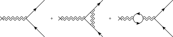
Figure 4: Diagrammatic topologies contributing to the vertex function up to one-loop order with $c^{\mu\nu}=0$. Counterterm contributions have been omitted for clarity.

It is straightforward but tedious to adapt the formulas for the tree-level cross sections (132) and (133) to the Lorentz-violating case accordingly. Rather than doing this explicitly, we will move our attention to radiative corrections. The diagrams shown in Fig. 4 contribute to one-loop order. Note that the fermion self-energy diagrams are taken into account implicitly in the order $\alpha$ corrections to the external spinors in formulas (118)–(124), as well as by the inclusion of the wave-function renormalization $\mathcal{Z}_{R}^{1/2}$ for each external fermion leg.

Instead of carrying out the full calculation of the one-loop diagrams, we will just concentrate on the infrared-divergent contributions to the scattering amplitude. We will then show that they indeed cancel in the experimental cross section, just as in the Lorentz-invariant case.

Paralleling the usual Lorentz-invariant case, the vacuum-polarization diagram is infrared finite, so that we only have to consider the vertex-correction diagram. With the modified photon propagator (recall that we have chosen $c^{\mu\nu}=0$) the amplitude for the vertex correction is given by

$$-iq\Gamma^{\mu}(p^{\prime},p)=(-iq)^{3}\mu^{\epsilon}\int\frac{d^{d}k}{(2\pi)^{d}}\frac{\gamma^{\alpha}i(\not{p}^{\prime}-\not{k}+m)\gamma^{\mu}i(\not{p}-\not{k}+m)\gamma^{\beta}(-i)(\eta_{\alpha\beta}-\tilde{k}_{\alpha\beta})}{\bigl{(}(p^{\prime}-k)^{2}-m^{2}+i\epsilon\bigr{)}\bigl{(}(p-k)^{2}-m^{2}+i\epsilon\bigr{)}\bigl{(}k^{2}+2\tilde{k}^{k}_{k}-m_{\gamma}^{2}+i\epsilon\bigr{)}}\,.$$ (136)

The integral on the right-hand side of Eq. (136) is infrared divergent. This divergence arises from the residue of the photon propagator. In order to isolate it, we can use the fermion on-shell relations $p^{2}-m^{2}=\mathcal{O}(\alpha)\approx 0$ and $(p^{\prime})^{2}-m^{2}=\mathcal{O}(\alpha)\approx 0$. It is then straightforward to show that

$$\bar{u}^{r}(p^{\prime})\gamma^{\alpha}(\not{p}^{\prime}+m)\gamma^{\mu}(\not{p}+m)\gamma^{\beta}u^{s}(p)(\eta_{\alpha\beta}-\tilde{k}_{\alpha\beta})=4\bar{u}^{r}(p^{\prime})\gamma^{\mu}u^{s}(p)(p^{\prime}\cdot p-\tilde{k}^{p^{\prime}}_{p})$$ (137)

by using the (approximate) equations of motion for the spinors. Moreover, we can drop terms linear in $k$ in the numerator and quadratic in $k$ in the fermion pole factors in the denominator. It then follows that

$$\bar{u}^{r}(p^{\prime})\Gamma^{\mu}(p^{\prime},p)u^{s}(p)\approx-iq^{2}\mu^{\epsilon}\bar{u}^{r}(p^{\prime})\gamma^{\mu}u^{s}(p)\int\frac{d^{d}k}{(2\pi)^{d}}\frac{p^{\prime}\cdot p-\tilde{k}^{p^{\prime}}_{p}}{k^{2}+2\tilde{k}^{k}_{k}-m_{\gamma}^{2}+i\epsilon}\frac{1}{(p^{\prime}\cdot k)(p\cdot k)}\,.$$ (138)

We can evaluate the integral (138) by using the identity

$$\frac{1}{k^{2}+2\tilde{k}^{k}_{k}-m_{\gamma}^{2}+i\epsilon}=\mbox{P}\frac{1}{k^{2}+2\tilde{k}^{k}_{k}-m_{\gamma}^{2}}-i\pi\delta(k^{2}+2\tilde{k}^{k}_{k}-m_{\gamma}^{2})\,,$$ (139)

where P denotes the principle-value part. Omitting the infrared-finite contribution from the principal value we find

$$\bar{u}^{r}(p^{\prime})\Gamma^{\mu}(p^{\prime},p)u^{s}(p)=-\frac{\alpha}{4\pi^{2}}\bar{u}^{r}(p^{\prime})\gamma^{\mu}u^{s}(p)\int d^{4}k\,\delta(k^{2}+2\tilde{k}^{k}_{k}-m_{\gamma}^{2})\frac{p^{\prime}\cdot p-\tilde{k}^{p^{\prime}}_{p}}{(p^{\prime}\cdot k)(p\cdot k)}.$$ (140)

It follows that the one-loop contributions to the elastic Coulomb scattering amplitude are obtained by substituting $\mathcal{M}_{0}\equiv\bar{u}^{s_{f}}(p_{f})\gamma^{0}u^{s_{i}}(p_{i})$ in Eq. (132) by

$$\mathcal{M}=\mathcal{M}_{0}\left\{1-\frac{\alpha}{4\pi^{2}}\int d^{4}k\delta(k^{2}+2\tilde{k}^{k}_{k}-m_{\gamma}^{2})\frac{p^{\prime}\cdot p-\tilde{k}^{p^{\prime}}_{p}}{(p^{\prime}\cdot k)(p\cdot k)}\right\}\mathcal{Z}_{R}^{1/2}(p^{\prime})\mathcal{Z}_{R}^{1/2}(p)+\cdots\,.$$ (141)

where the ellipsis indicates infrared-finite contributions. For the elastic cross section, this implies

$$\frac{d\sigma_{fi}^{el}}{d\Omega}=\frac{d\sigma_{fi}^{0}}{d\Omega}\left\{1-\frac{\alpha}{2\pi^{2}}\int d^{4}k\delta(k^{2}+2\tilde{k}^{k}_{k}-m_{\gamma}^{2})\frac{p^{\prime}\cdot p-\tilde{k}^{p^{\prime}}_{p}}{(p^{\prime}\cdot k)(p\cdot k)}\right\}\mathcal{Z}_{R}(p^{\prime})\mathcal{Z}_{R}(p)+\cdots\,.$$ (142)

The term proportional to $\alpha$ as well as the factors $\mathcal{Z}_{R}$ in expression (142) are infrared divergent for $m_{\gamma}\to 0$.

In the Lorentz-invariant case, infrared divergences are canceled if one incorporates the fact that some final states that include soft photons are experimentally indistinguishable. We will now proceed to check that this continues to hold true in the case at hand.

Following the usual procedure, we consider final states that include one soft photon with energy smaller than the detector resolution $\Delta E$. The amplitude for this process is

$$\mathcal{M}=q\mathcal{M}_{0}\left[\frac{2p^{\prime}\cdot\epsilon_{r}}{2p^{\prime}\cdot k}+\frac{2p\cdot\epsilon_{r}}{-2p\cdot k}\right]\,,$$ (143)

where $\mathcal{M}_{0}$ is the amplitude for elastic scattering without photon emission. To get the cross section for this process, we have to include also the final-state volume element for the photon. As shown in Appendix D, a consistent way to do this is to take

$$\frac{d^{3}k}{(k_{0+}+k_{0-})(2\pi)^{3}}$$ (144)

rather than the conventional factor $d^{3}k/(2\omega_{k}(2\pi)^{3})$. Here, $k_{0\pm}(\vec{k})$ are the absolute values of the solutions for $k_{0}$ to the modified dispersion relation.

Combining Eqs. (143) and (144) and employing formula (207) one then finds for the cross section for this (soft-bremsstrahlung) process

$$\frac{d\sigma_{fi}^{1\gamma}}{d\Omega}\approx\frac{d\sigma_{fi}^{0}}{d\Omega}\frac{q^{2}}{2(2\pi)^{3}}\int_{\omega\leq\Delta E}d^{4}k\,\tilde{\eta}^{00}\delta^{4}\bigl{(}k^{2}+\tilde{k}^{k}_{k}-m_{\gamma}^{2}\bigr{)}\sum_{\lambda=1}^{3}\left[\frac{2p^{\prime}\cdot\epsilon^{(\lambda)}(k)}{2p^{\prime}\cdot k}+\frac{2p\cdot\epsilon^{(\lambda)}(k)}{-2p\cdot k}\right]^{2}.$$ (145)

Using the polarization-sum formula (206), Eq. (145) reduces to

$$\frac{d\sigma_{fi}^{1\gamma}}{d\Omega}\approx\frac{d\sigma_{fi}^{0}}{d\Omega}\frac{\alpha}{(2\pi)^{2}}\int_{\omega\leq\Delta E}d^{4}k\,\delta^{4}\bigl{(}k^{2}+\tilde{k}^{k}_{k}-m_{\gamma}^{2}\bigr{)}\left[-\frac{(p^{\prime})^{2}-\tilde{k}^{p^{\prime}}_{p^{\prime}}}{(p^{\prime}\cdot k)^{2}}-\frac{p^{2}-\tilde{k}^{p}_{p}}{(p\cdot k)^{2}}+\frac{2p^{\prime}\cdot p-2\tilde{k}^{p^{\prime}}_{p}}{(p^{\prime}\cdot k)(p\cdot k)}\right].$$ (146)

Comparing the third term inside brackets in Eq. (146) with Eq. (142) we see that both contain integrals over the same $p,p^{\prime}$ term, with opposite sign, so that the corresponding infrared divergences cancel.

To verify that the same happens for the $p,p$ and the $p^{\prime},p^{\prime}$ terms in Eq. (146) and the $\mathcal{Z}_{R}(p^{\prime})\mathcal{Z}_{R}(p)$ factors in Eq. (142), we evaluate the $k$ integral over, say, the $p,p$ term in Eq. (146). To this end, we perform a change of variables $k^{\mu}\to\bar{k}^{\mu}$ such that

$$\bar{k}^{2}=k^{2}+\tilde{k}^{k}_{k}\,.$$ (147)

To first order, this means that $\bar{k}^{\mu}=k^{\mu}+\frac{1}{2}\tilde{k}^{\mu\nu}k_{\nu}$. To lowest order, the measure $d^{4}k$ is invariant under this transformation, as

$$\mbox{Det}\left[\frac{\partial\bar{k}}{\partial k}\right]\approx\mbox{Det}\Bigl{[}\delta^{\mu}_{\nu}+\frac{1}{2}\tilde{k}^{\mu}_{\nu}\Bigr{]}\approx 1+\frac{1}{2}\tilde{k}^{\mu}_{\mu}=1\,.$$ (148)

It follows that

$$\int_{\omega\leq\Delta E}d^{4}k\,\delta\bigl{(}k^{2}+\tilde{k}^{k}_{k}-m_{\gamma}^{2}\bigr{)}\frac{p^{2}-\tilde{k}^{p}_{p}}{(p\cdot k)^{2}}$$

$$\approx\int_{\bar{\omega}\leq\Delta E}d^{4}\bar{k}\,\delta(\bar{k}^{2}-m_{\gamma}^{2})\frac{\tilde{p}^{2}}{(\bar{k}\cdot\tilde{p})^{2}}\,,$$ (149)

where we have defined $\tilde{p}^{\mu}=(\eta^{\mu\nu}-\frac{1}{2}\tilde{k}^{\mu\nu})p_{\nu}$. Note that strictly speaking, the upper limit of the transformed energy $\bar{\omega}$ is modified by the transformation, but the result is an effect of higher order in $\tilde{k}$ and can be ignored. The resulting integration is a standard one with result, Itzykson

$$4\pi\ln\left(\frac{\Delta E}{m_{\gamma}}\right)+\cdots\,,$$ (150)

where the ellipsis indicates terms that are finite as $m_{\gamma}\to 0$. Substitution in Eq. (146) gives (for the second term)

$$-\frac{d\sigma_{fi}^{0}}{d\Omega}\,\frac{\alpha}{\pi}\ln\left(\frac{\Delta E}{m_{\gamma}}\right)+\mbox{finite}.$$ (151)

It follows that the infrared divergence in Eq. (151) indeed cancels the corresponding one in the elastic cross section (142) arising from the multiplicative renormalization function $\mathcal{Z}_{R}(p)$ that was evaluated in Eq. (81):

$$\mathcal{Z}_{R}\bigl{(}(c,k)^{p}_{p}\bigr{)}=1+\frac{\alpha}{\pi}\ln\left(\frac{m}{m_{\gamma}}\right)+\mbox{finite}.$$ (152)

VII Summary and outlook

Perturbative Lorentz-invariant quantum field theory rests on a few core field-theoretic techniques. One of these concerns the order-by-order determination of the asymptotic Hilbert space, and thus the calculation of quantum corrections to the external states. Such effects govern the propagation of free particles and are indispensable for scattering amplitudes. The present work for the first time has addressed the issue how to generalize this core technique to Lorentz-violating quantum-field theories. To illustrate the salient features of this generalization, we have focused on a particular sector of the SME. We expect, though, that our reasoning can also be applied to other Lorentz-violating field theories with a more complex structure and a wider variety of coefficients.

Specifically, we considered the SME’s single-flavor QED sector in the presence of the $c^{\mu\nu}$ and the nonbirefringent piece of the $k_{F}^{\mu\nu\alpha\beta}$ coefficients. Working perturbatively, we found that the presence of these Lorentz-breaking terms in the Lagrangian has some profound consequences for the radiative corrections to the pole structure of the external states. In particular, the Dirac equation satisfied by the external-state spinors turns out to be modified by Lorentz-violating operators not present in the Lagrangian, a feature that is unknown in usual Lorentz-symmetric field theories. Our analysis also shows that the wave-function renormalization will typically contain Lorentz-breaking coefficients contracted with momenta. We note that this is in contrast to the usual one-loop QED result, where $Z_{\psi}$ is a momentum-independent constant. Momentum dependence of the wave-function renormalization is known to occur in certain other contexts momemtum_dep_Z .

We have limited our present study primarily to theoretical techniques for determining quantum corrections to external states in Lorentz-violating backgrounds. However, our results indicate that such corrections may have profound phenomenological implications for Lorentz tests, which can be seen as follows. The new, radiatively induced term exhibits two powers of the momentum, whereas the existing terms contain only up to a single power. The correction term should therefore grow faster with the momentum than the existing terms. This opens the possibility—at least in principle—that the Lorentz-breaking radiative corrections become larger than the original tree-level Lorentz violation. Note that this does not necessarily signal a breakdown of perturbation theory because the perturbation Hamiltonian also includes the conventional electromagnetic interaction, which is comparatively much larger.

In our simple model, the radiative-correction term of size $\sim\frac{\alpha}{3\pi m}(2c^{p}_{p}-\tilde{k}^{p}_{p})$ can reach the size of the tree-level contribution $c^{p}_{\gamma}$ when $\alpha\,p\sim m$. It follows that for Lorentz tests involving free electrons with energies $\mathrel{\hbox to0.0pt{\lower 3.0pt\hbox{$\sim$}\hss}\raise 2.0pt\hbox{$>$}}100\;$MeV, radiative Lorentz-breaking corrections may not always be negligible relative to the tree-level Lorentz violation. Note that electrons in such an energy range are routinely employed in various Lorentz tests. We remark, however, that in our particular model the resulting fermion eigenenergies are free of this effect. This may be a special property of our model as both the tree-level Lorentz violation and the induced correction have the same C, P, and T properties. Nevertheless, the model discussed in this work could still exhibit other observables, such as ones involving the one-loop eigenspinors, in which the Lorentz-breaking correction dominates the tree-level effects. In the context of more general models involving the parity-odd weak interaction, the radiatively induced terms are likely to display a greater variety of structures since they do not necessarily have to share the same C, P, and T properties of the tree-level Lorentz violation. Then, even the eigenenergies may show the effects mentioned above.

Another immediate consequence of our result concerns multimetric theories multimetric , such as recently proposed bimetric models bimetric ; bimcrit . The basic idea in models of this type is that different fields experience different effective metrics. But our analysis shows that the concept of two metrics is difficult to maintain in a quantum theory: beyond tree level, radiative corrections to particle propagation typically induce higher-order terms incompatible with an effective-metric interpretation. This difficulty by itself does not affect the consistency of such models; it rather illustrates, for example, that the trajectory of the particle is not a geodesic with respect to some metric.

To see this more explicitly, consider first the free electromagnetic field in our model. Inspection of Eqs. (6) and (7) establishes that $\hat{\eta}^{\mu\nu}=\eta^{\mu\nu}+\tilde{k}^{\mu\nu}$ can be interpreted as the effective (inverse) metric that governs photon propagation at tree level. Similarly, comparison of our fermion kinetic term ${\textstyle\frac{1}{2}}i\overline{\psi}(\delta^{\mu}_{a}+c^{\mu}_{a})\gamma^{a}\!\!\!\stackrel{{\scriptstyle\;\leftrightarrow}}{{\partial}}_{\!\!\mu}\!\!\psi$ with that in general coordinates ${\textstyle\frac{1}{2}}ie\overline{\psi}e^{\mu}_{a}\gamma^{a}\!\!\!\stackrel{{\scriptstyle\;\leftrightarrow}}{{\partial}}_{\!\!\mu}\!\!\psi$ reveals that we may interpret $\delta^{\mu}_{a}+c^{\mu}_{a}$ as the vierbein $e^{\mu}_{a}$ c=const_comment . It is then apparent that the fermion propagation is controlled by the (inverse) effective metric $(g_{f})^{\mu\nu}=e^{\mu}_{a}e^{\nu}_{b}\eta^{ab}=\eta^{\mu\nu}+2c^{\mu\nu}+{\cal O}(c^{2})$ at tree level. We see that in the absence of quantum corrections our Lorentz-violating QED extension can indeed be interpreted as a bimetric model in the flat-spacetime limit. We remark in passing that this is consistent with our earlier discussion that only $2c^{\mu\nu}-\tilde{k}^{\mu\nu}$ is observable. On the other hand, our analysis has shown that the leading radiative corrections to the free-fermion propagation—displayed in Eq. (84)—are determined by a term of the form $\overline{\psi}(2c^{\mu\nu}-\tilde{k}^{\mu\nu})\partial_{\mu}\partial_{\nu}\psi$. But such a term precludes an interpretation of the fermion’s propagation as being governed by an effective metric.

On a more practical level, we applied our formalism to Coulomb scattering for the case $c^{\mu\nu}=0$, $\tilde{k}^{\mu\nu}\neq 0$. We showed that, just like in the usual Lorentz-symmetric case, infrared divergences cancel when soft-photon emission is taken into account in the final fermion states. It should be stressed that this result involves a nontrivial cancellation between various infrared-divergent Lorentz-violating terms. Our study also demonstrates how to extract the S-matrix of a process with external fermion states in the presence of Lorentz-breaking coefficients, generalizing the usual LSZ reduction formula to incorporate leading-order SME effects.

In this paper, we have only considered linear Lorentz-violating radiative effects on fermion external states, which suggests two natural avenues for further exploration. One of these concerns a nonperturbative treatment of asymptotic states at all orders in Lorentz breaking within formal field theory. A study of this kind could yield additional theoretical insight, such as the analytic structure of the single-particle propagator away from the pole. The second avenue for future investigations involves photon-propagation effects, and in particular the incorporation of Lorentz breakdown into vacuum polarization. An analysis along these lines needs to include a study of the Källén–Lehmann representation for the photon propagator in the presence of the full $k_{F}^{\mu\nu\alpha\beta}$ coefficient to facilitate a proper extraction of the photon pole(s). We expect to return to this issue in the future.

Appendix A Feynman rules for the second perturbation scheme

This appendix presents the Feynman rules needed for perturbative calculations in our model. In Sec. III, we briefly discussed two natural schemes for setting up perturbation theory, each entailing different decompositions of our model’s full Lagrangian and the ensuing different sets of Feynman rules for each scheme. For convenience, we selected as the zeroth-order system the full renormalized quadratic Lagrangian (including quadratic Lorentz-violating pieces) and to treat the nonquadratic terms as a perturbation. The Feynman rules for this choice, i.e., for decomposition corresponding to Eqs. (15), (16), and (17), are displayed in Fig. 5, where we have selected $\xi=1$ Feynman gauge. Counterterm expressions, which are not displayed here, have been taken from Ref. Kostelecky:2001jc .

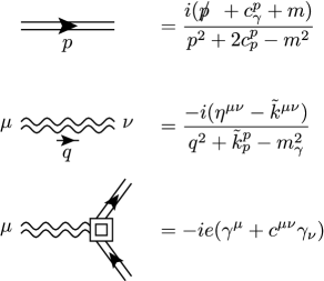
Figure 5: Feynman rules in $\xi=1$ gauge for the decomposition of our Lagrangian according to Eqs. (15), (16), and (17). Counterterm insertions are not shown.

Appendix B Expansion of $\bm{\Gamma^{(2)}(\bar{P})}$

We begin by considering the expression (38) for $\Gamma^{(2)}(\bar{P})$, which shows that expansions of the scalar coefficient functions $A$, $C$, $K$, and $M$ are needed,

$$A(\bar{P}^{2}+ 2\bar{m}\bar{P}+\bar{\beta},c^{p}_{p},\tilde{k}^{p}_{p})=$$

$$\sum_{n=0}^{\infty}\frac{1}{n!}A^{(n)}(\bar{\beta},c^{p}_{p},\tilde{k}^{p}_{p})(\bar{P}^{2}+2\bar{m}\bar{P})^{n}\,,$$ (153)

with analogous expressions for $C$, $K$, and $M$. Here, we have denoted the $n$th derivative with respect to the first argument by the superscript $(n)$. No ordering ambiguities arise at this stage, because the only nontrivial matrix in all of these expansions is $\bar{P}$.

More care is required when the expansions for $A$, $C$, $K$, and $M$ are inserted into the expression (38) for $\Gamma^{(2)}(\bar{P})$ because the expansions are then multiplied by $c^{p}_{\gamma}$ and $\tilde{k}^{p}_{\gamma}$, and these two matrices do in general not commute with $\bar{P}$. However, by virtue of Eq. (36) we see that $(\bar{P}^{2}+2\bar{m}\bar{P})=p^{2}-\bar{\beta}$ is proportional to $\openone$ and thus commutes with any matrix. Therefore, we may write for $n\geq 2$,

$$c^{p}_{\gamma}(\bar{P}^{2} +2\bar{m}\bar{P})^{n}=$$

$$\bar{P}\Big{[}(\bar{P}+2\bar{m})c^{p}_{\gamma}(\bar{P}^{2}+2\bar{m}\bar{P})^{n-2}(\bar{P}+2\bar{m})\Big{]}\bar{P}\,,$$ (154)

with analogous expressions for $C$, $K$, and $M$, as well as $c^{p}_{\gamma}$ replaced by $\tilde{k}^{p}_{\gamma}$. This implies that all terms with $n\geq 2$ in our above expansion of $\Gamma^{(2)}(\bar{P})$ take the generic form $\bar{P}[\ldots]\bar{P}$, where the square brackets contain some matrix polynomial in $p^{\mu}$. But terms of this form can be ignored for the purpose of extracting the pole structure, as is apparent from our discussion in the context of Eqs. (24) and (25).

The structure of the pole is governed by the remaining terms corresponding to $n=0,1$. At this point, the order of various matrices must be determined carefully. Consider, for example, the term

$$C^{\prime}(\bar{\beta},c^{p}_{p},\tilde{k}^{p}_{p})(\bar{P}^{2}+2\bar{m}\bar{P})c^{p}_{\gamma}\,,$$ (155)

which represents the $n=1$ contribution to the fourth line in Eq. (38). In this expression, $c^{p}_{\gamma}$ and $(\bar{P}^{2}+2\bar{m}\bar{P})$ may still be interchanged freely, but the pole is determined by terms linear in $\bar{P}$. One might then be tempted simply to drop $\bar{P}^{2}$ contributions. However, this yields either $2\bar{m}C^{\prime}(\bar{\beta},c^{p}_{p},\tilde{k}^{p}_{p})\bar{P}c^{p}_{\gamma}$ or $2\bar{m}C^{\prime}(\bar{\beta},c^{p}_{p},\tilde{k}^{p}_{p})c^{p}_{\gamma}\bar{P}$ depending on the choice of matrix ordering in the original $n=1$ term (155). Moreover, regardless of which one of these two choices is adopted, the resulting expression fails to be of the form ${\cal Z}^{-1}_{R}\bar{P}$ required by Eq. (25) , where ${\cal Z}^{-1}_{R}$ is a number and not a matrix.

The basic idea behind the selection of the proper ordering is as follows. We parametrize all possible ordering choices, arrange this general expression into series in $\bar{P}$, and then fix the parameter (and thus the ordering choice) such that an expression with the structure demanded by Eq. (25) emerges. Let us demonstrate this idea explicitly for the above sample term (155), where we may ignore the $C^{\prime}(\bar{\beta},c^{p}_{p},\tilde{k}^{p}_{p})$ coefficient in the present context. We write

$$(\bar{P}^{2}+2\bar{m}\bar{P})c^{p}_{\gamma} = \zeta(\bar{P}^{2}+2\bar{m}\bar{P})c^{p}_{\gamma}$$ (156)

$${}+(1-\zeta)c^{p}_{\gamma}(\bar{P}^{2}+2\bar{m}\bar{P})$$

$$= 2\zeta(2c^{p}_{p}\bar{P}-\bar{P}c^{p}_{\gamma}\bar{P})$$

$${}+(1-2\zeta)c^{p}_{\gamma}(\bar{P}^{2}+2\bar{m}\bar{P})\,,$$

where $\zeta$ is a free coefficient parametrizing the matrix ordering. To arrive at the last equality, we have employed the result $\{\bar{P}^{2}+2\bar{m}\bar{P},c^{p}_{\gamma}\}=4c^{p}_{p}\bar{P}-2\bar{P}c^{p}_{\gamma}\bar{P}$, which follows from an explicit evaluation of the anticommutator. The next step is to fix $\zeta$ by requiring compatibility with Eq. (25). This is achieved by choosing $\zeta=\frac{1}{2}$, which eliminates the offending terms in the last line. We conclude that the following symmetrized representation of Eq. (38),

$$\Gamma^{(2)}(\bar{P}) = A(\bar{P}{}^{2}+2\bar{m}\bar{P}+\bar{\beta},c^{p}_{p},\tilde{k}^{p}_{p})\bar{P}$$ (157)

$${}+\bar{m}A(\bar{P}{}^{2}+2\bar{m}\bar{P}+\bar{\beta},c^{p}_{p},\tilde{k}^{p}_{p})\openone$$

$${}-M(\bar{P}{}^{2}+2\bar{m}\bar{P}+\bar{\beta},c^{p}_{p},\tilde{k}^{p}_{p})\openone$$

$${}+{\textstyle\frac{1}{2}}\big{\{}C(\bar{P}{}^{2}+2\bar{m}\bar{P}+\bar{\beta}),c^{p}_{\gamma}\big{\}}$$

$${}-{\textstyle\frac{1}{2}}\bar{x}\big{\{}A(\bar{P}{}^{2}+2\bar{m}\bar{P}+\bar{\beta},c^{p}_{p},\tilde{k}^{p}_{p}),c^{p}_{\gamma}\big{\}}$$

$${}+{\textstyle\frac{1}{2}}\big{\{}K(\bar{P}{}^{2}+2\bar{m}\bar{P}+\bar{\beta}),\tilde{k}^{p}_{\gamma}\big{\}}$$

$${}-{\textstyle\frac{1}{2}}\bar{y}\big{\{}A(\bar{P}{}^{2}+2\bar{m}\bar{P}+\bar{\beta},c^{p}_{p},\tilde{k}^{p}_{p}),\tilde{k}^{p}_{\gamma}\big{\}}\,,\qquad$$

possesses the proper matrix ordering when an expansion in powers of $\bar{P}$ with the structure (25) is desired.

From a practical perspective, the above discussion implies that we may replace

$${\textstyle\frac{1}{2}}\big{\{}C(\bar{P}{}^{2}+2\bar{m}\bar{P}+\bar{\beta}),c^{p}_{\gamma}\big{\}}\to C(\bar{\beta})c^{p}_{\gamma}+2C^{\prime}(\bar{\beta})c^{p}_{p}\bar{P}$$ (158)

for the purpose of extracting the pole with analogous relations for the remaining anticommutators in Eq. (157). To leading order in Lorentz violation, we find

$$\Gamma^{(2)}(\bar{P}) = {}+\Big{[}\bar{m}A(\bar{\beta},c^{p}_{p}\tilde{k}^{p}_{p})\openone-M(\bar{\beta},c^{p}_{p},\tilde{k}^{p}_{p})\openone$$ (159)

$$\hskip 20.00003pt{}+C(m_{\rm ph}^{2})c^{p}_{\gamma}-\bar{x}A(m_{\rm ph}^{2})c^{p}_{\gamma}$$

$$\hskip 20.00003pt{}+K(m_{\rm ph}^{2})\tilde{k}^{p}_{\gamma}-\bar{y}A(m_{\rm ph}^{2})\tilde{k}^{p}_{\gamma}\Big{]}$$

$${}+\Big{[}A(\bar{\beta},c^{p}_{p},\tilde{k}^{p}_{p})+2\bar{m}^{2}A^{\prime}(\bar{\beta},c^{p}_{p},\tilde{k}^{p}_{p})$$

$$\hskip 20.00003pt{}-2\bar{m}M^{\prime}(\bar{\beta},c^{p}_{p},\tilde{k}^{p}_{p})$$

$$\hskip 20.00003pt{}-2\bar{x}A^{\prime}(m_{\rm ph}^{2})c^{p}_{p}-2\bar{y}A^{\prime}(m_{\rm ph}^{2})\tilde{k}^{p}_{p}$$

$$\hskip 20.00003pt{}+2C^{\prime}(m_{\rm ph}^{2})c^{p}_{p}+2K^{\prime}(m_{\rm ph}^{2})\tilde{k}^{p}_{p}\Big{]}\bar{P}$$

$${}+\bar{P}[\ldots]\bar{P}\,,\qquad$$

where we have employed the same notation as in Eqs. (40) and (41). The first square bracket needs to vanish since $\Gamma^{(2)}(0)=0$ at the pole. We thus recover the result (39). The second square bracket is identified as ${\cal Z}^{-1}_{R}$.

Appendix C Quantization of the Dirac field in the presence of Lorentz violation

In this appendix, we carry out the explicit quantization of the Dirac field in the presence of Lorentz violation. One possible approach is to use a field redefinition $\psi=A\chi$ that transforms the terms with time derivatives to the standard Dirac form fermion-field-redefinition ; quant1 . Alternatively, one may use an unconventional scalar product in spinor space to bypass the Hermiticity issues associated with unconventional time derivatives (Kostelecky:2010ze, ). The method presented below is based on this latter approach, is more direct, maintains spinor coordinate covariance, is more direct, maintains spinor coordinate covariance, and introduces explicit creation and annihilation operators for the particle modes corresponding to the physical field $\psi$ as well as an expression for the Hamiltonian in terms of these. These features are particularly suitable for the quantization of the spinor equation of motion (100).

We start with the free-fermion Lagrange density

$$\mathcal{L}_{f}=\bar{\psi}(i\Gamma^{\mu}\partial_{\mu}-M)\psi\,,$$ (160)

with

$$\Gamma^{\mu}= \,\,\gamma^{\mu}+c^{\mu\nu}\gamma_{\nu}+d^{\mu\nu}\gamma_{5}\gamma_{\nu}+if^{\mu}\gamma_{5}+\frac{1}{2}g^{\lambda\nu\mu}\sigma_{\lambda\nu}+e^{\mu}\,,$$ (161)

$$M= \,\,m+a^{\mu}\gamma_{\mu}+b^{\mu}\gamma_{5}\gamma_{\mu}+{1\over 2}H^{\mu\nu}\sigma_{\mu\nu}\,.$$ (162)

The Lorentz-violating background is taken as real valued, so that $\Gamma^{\mu}{}^{\dagger}=\gamma^{0}\Gamma^{\mu}\gamma^{0}$ and $M^{\dagger}=\gamma^{0}M\gamma^{0}$. The canonical momentum is given by

$$\pi=\frac{\partial_{R}\mathcal{L}_{f}}{\partial{\dot{\psi}}}=i\bar{\psi}\Gamma^{0}\,,$$ (163)

and the canonical Hamiltonian becomes

$$H= \int d^{3}x\bigl{[}\pi\dot{\psi}-\mathcal{L}_{f}\bigr{]}=\int d^{3}x\,\bar{\psi}(-i\,\vec{\Gamma}\!\cdot\!\vec{\nabla}+M)\psi$$

$$= \int d^{3}x\,\pi(\Gamma^{0})^{-1}(-\vec{\Gamma}\!\cdot\!\vec{\nabla}-iM)\psi\,.$$ (164)

The matrix $\Gamma^{0}$ is indeed invertible for perturbatively small Lorentz violation quant1 . From this Hamiltonian, one can recover the equation of motion

$$\dot{\psi}(x)=\frac{\delta H}{\delta\pi(x)}=(\Gamma^{0})^{-1}(-\vec{\Gamma}\!\cdot\!\vec{\nabla}-iM)\psi\,.$$ (165)

Next, we expand the solutions of the equation of motion for $\psi$ in Fourier modes,

$$\psi(x)= \int\!\frac{d^{3}\vec{p}}{(2\pi)^{3}}\,\frac{m}{\omega_{p}}\sum_{s=1,2}\!\!\big{[}b_{s}(\vec{p})u^{s}(\vec{p})e^{-ip\cdot x}$$

$$\hskip 100.00015pt+d_{s}^{\dagger}(\vec{p})v^{s}(\vec{p})e^{ip\cdot x}\big{]}\,,$$ (166)

where $\omega_{p}\equiv+(m^{2}+\vec{p}^{\,2})^{1/2}$ denotes the conventional fermion energies, and $p^{0}$ takes the absolute value of the respective (four) eigenvalues of $(\Gamma^{0})^{-1}(\Gamma^{i}p^{i}+M)$. The latter are, in general, all different. But for small enough Lorentz-violating parameters, two of them (which we will denote $p^{0}_{u,s}$) are positive, and two ($-p^{0}_{v,s}$) are negative quant1 . Below, we will show that these eigenvalues are, in fact, real. The corresponding eigenvectors are $u^{s}(\vec{p})$ and $v^{s}(\vec{p})$, which satisfy

$$(\Gamma^{\mu}p_{\mu}-M)u^{s}(\vec{p})=0\,,\quad(\Gamma^{\mu}p_{\mu}+M)v^{s}(\vec{p})=0\,.$$ (167)

Here, Latin superscripts $r,s,\ldots$ from the middle of the alphabet label the spin-type state. To quantize, we replace the Poisson brackets with $i\times$anticommutators:

$$[\psi_{a}(\vec{x},t),\bar{\psi}_{b}(\vec{y},t)]_{+}= \;[\psi_{a}(\vec{x},t),-i\pi_{c}(\vec{y},t)]_{+}(\Gamma^{0})^{-1}_{cb}$$

$$= \;(\Gamma^{0})^{-1}_{ab}\delta^{3}(\vec{x}-\vec{y})$$ (168)

and

$$[\psi_{a}(\vec{x},t),\psi_{b}(\vec{y},t)]_{+}=[\bar{\psi}_{a}(\vec{x},t),\bar{\psi}_{b}(\vec{y},t)]_{+}=0\,,$$ (169)

where Latin subscripts $a,b,c,\ldots$ from the beginning of the alphabet denote spinor components. We now proceed to check that the anticommutation relations (168) and (169) correspond to taking for the oscillators the following nonzero anticommutators:

$$[b_{r}(\vec{p}),b_{s}^{\dagger}(\vec{q})]_{+}=[d_{r}(\vec{p}),d_{s}^{\dagger}(\vec{q})]_{+}=(2\pi)^{3}\frac{\omega_{p}}{m}\delta^{3}(\vec{q}-\vec{p})\,\delta_{rs}\,.$$ (170)

With these relations, we find from Eq. (166),

$$[\psi_{a}(\vec{x},t),\bar{\psi}_{b}(\vec{y},t)]_{+}= \int\!\frac{d^{3}\vec{p}}{(2\pi)^{3}}\,\frac{m}{\omega_{p}}\sum_{s}\big{[}u_{a}^{s}(\vec{p})\bar{u}_{b}^{s}(\vec{p})$$

$${}+v^{s}_{a}(-\vec{p})\bar{v}^{s}_{b}(-\vec{p})\big{]}e^{+i\vec{p}\cdot(\vec{x}-\vec{y})}\,.$$ (171)

To see that the matrix $\Gamma_{0}^{-1}(\vec{\Gamma}\!\cdot\!\vec{p}+M)$ has real eigenvalues, we note that

$$\langle u|v\rangle\equiv\bar{u}\Gamma^{0}v$$ (172)

represents an (unconventional) inner product on spinor space. In this expression, $u$ and $v$ are arbitrary spinors with the usual notation $\bar{u}\equiv u^{\dagger}\gamma^{0}$. The definition (172) clearly satisfies the appropriate linearity conditions of an inner product. To establish positive definiteness, note first that $\bar{u}\Gamma^{0}u$ is always real since $(\Gamma^{0})^{\dagger}=\gamma^{0}\Gamma^{0}\gamma^{0}$. Moreover, $\gamma^{0}\Gamma^{0}$ differs from $\openone$ only by SME corrections, which implies positive definiteness for sufficiently small Lorentz violation quant1 . The matrix $\Gamma_{0}^{-1}(\vec{\Gamma}\!\cdot\!\vec{p}+M)$ turns out to be Hermitian with respect to the modified inner product (172), which shows that this matrix indeed possesses real eigenvalues, as claimed. Moreover, the presumed small size of the SME corrections implies that these eigenvalues are perturbations around the conventional ones, so two eigenenergies are positive and two negative quant1 . The four corresponding eigenspinors are orthogonal and can be normalized in the usual way:

$$\bar{u}^{r}(\vec{p})\Gamma^{0}u^{s}(\vec{p})=\bar{v}^{r}(-\vec{p})\Gamma^{0}v^{s}(-\vec{p})=\frac{\omega_{p}}{m}\,\delta_{rs}\,.$$ (173)

As $\{u^{1}(\vec{p}),u^{2}(\vec{p}),v^{1}(-\vec{p}),v^{2}(-\vec{p})\}$ forms a complete set of eigenspinors of the operator $(\Gamma^{0})^{-1}(\vec{\Gamma}\!\cdot\!\vec{p}+M)$, we have the completeness relation

$$\sum_{s=1}^{2}\big{[}u^{s}_{a}(\vec{p})\bar{u}^{s}_{c}(\vec{p})+v^{s}_{a}(-\vec{p})\bar{v}^{s}_{c}(-\vec{p})\big{]}\Gamma^{0}_{cb}=\frac{\omega_{p}}{m}\;\delta_{ab}\,.$$ (174)

We can now use this completeness relation in Eq. (171), recovering the result of Eq. (168).

As a further application, let us derive an expression for the Hamiltonian in terms of the oscillators. The quantum-field version of Eq. (164) is given by

$$H=\int\!d^{3}x\,:\bar{\psi}(-i\,\vec{\Gamma}\!\cdot\!\vec{\nabla}+M)\psi:\,.$$ (175)

With the Fourier decomposition (166) we find, using the equations of motion (167) for $u^{s}(\vec{p})$ and $v^{s}(\vec{p})$, an explicitly positive-definite expression for the Hamiltonian,

$$H=\int\!\frac{d^{3}\vec{p}}{(2\pi)^{3}}\,\frac{m}{\omega_{p}}\sum_{s=1}^{2}\big{[}E^{s}_{u}b_{s}^{\dagger}(\vec{p})b_{s}(\vec{p})+E^{s}_{v}d_{s}^{\dagger}(\vec{p})d_{s}(\vec{p})\big{]}\,,$$ (176)

where $E^{s}_{u}$ and $E^{s}_{v}$ are the (positive) energies corresponding to the solutions of Eq. (167). We also note the useful expressions

$$b_{s}^{\dagger}(\vec{p}) = \int\!d^{3}x\,e^{-ip\cdot x}\bar{\psi}(x)\Gamma^{0}u^{s}(\vec{p})\,,$$ (177)

$$d_{s}^{\dagger}(\vec{p}) = \int\!d^{3}x\,e^{-ip\cdot x}\bar{v}_{s}(\vec{p})\Gamma^{0}\psi(x)\,,$$ (178)

and their Hermitian conjugates.

The time-ordered product is defined in the usual way Tprod and satisfies

$$T\psi_{a}(x)\bar{\psi}_{b}(y)=\langle 0|T\psi_{a}(x)\bar{\psi}_{b}(y)|0\rangle+:\psi_{a}(x)\bar{\psi}_{b}(y):\,,$$ (179)

where

$$\langle 0|T\psi_{a}(x)\bar{\psi}_{b}(y)|0\rangle\equiv iS(x-y)_{ab}$$ (180)

is the modified Feynman propagator:

$$S(x-y)=\int\frac{d^{4}k}{(2\pi)^{4}}\frac{e^{-ik\cdot(x-y)}}{\Gamma^{\mu}k_{\mu}-M+i\epsilon}\,.$$ (181)

Indeed, one can verify that

$$(i\Gamma^{\mu}\partial_{\mu}-M)\langle 0|T\psi(x)\bar{\psi}(y)|0\rangle=i\delta^{4}(x-y)\,.$$ (182)

Here, we used that $\psi(x)$ satisfies the modified Dirac equation (165) and the anticommutator relation (168).

Appendix D Canonical quantization of the radiation field with Lorentz-violating parameter $\bm{\tilde{k}^{\mu\nu}}$

Our starting point is the following Lorentz-violating Stueckelberg Lagrange density in $\xi=1$ Feynman gauge,

$$\mathcal{L}_{\gamma}=-\tfrac{1}{4}\tilde{\eta}^{\alpha\beta}\tilde{\eta}^{\mu\nu}F_{\alpha\mu}F_{\beta\nu}-\tfrac{1}{2}(\partial_{\mu}\tilde{\eta}^{\mu\nu}\!A_{\nu})^{2}+\tfrac{1}{2}m_{\gamma}^{2}A_{\mu}\tilde{\eta}^{\mu\nu}\!A_{\nu}\,,$$ (183)

where $\tilde{\eta}^{\mu\nu}=\eta^{\mu\nu}+\tilde{k}^{\mu\nu}$, with $\tilde{k}^{\mu\nu}=\tilde{k}^{\nu\mu}$ and $\tilde{k}^{\mu}{}_{\mu}=0$. The quantization of such photon models has recently been studied by various authors (quant3, ). Here, we summarize the main results and tailor the presentation to the case at hand.

We begin by finding the canonical momenta

$$\Pi^{\mu}=\frac{\partial\mathcal{L}}{\partial(\partial_{0}A_{\mu})}=\tilde{\eta}^{\mu\alpha}\tilde{\eta}^{0\beta}F_{\alpha\beta}-\tilde{\eta}^{0\mu}(\partial_{\mu}\tilde{\eta}^{\mu\nu}A_{\nu})\,,$$ (184)

and impose the fundamental equal-time commutation relations

$$[A_{\mu}(t,\vec{x}),A_{\nu}(t,\vec{y})] =[\Pi^{\mu}(t,\vec{x}),\Pi^{\nu}(t,\vec{y})]=0\,,$$ (185)

$$[A_{\mu}(t,\vec{x}),\Pi^{\nu}(t,\vec{y})] =i\delta_{\mu}^{\nu}\delta^{3}(\vec{x}-\vec{y})\,.$$ (186)

From Eq. (185) it follows that the spatial derivatives of $A_{\mu}$ commute at equal times. Using Eqs. (186) and (184), one then deduces that

$$[\dot{A}_{\mu}(t,\vec{x}),A_{\nu}(t,\vec{y})]=i(\tilde{\eta}^{00})^{-1}\bar{\eta}_{\mu\nu}\delta^{3}(\vec{x}-\vec{y})\,,$$ (187)

where $\bar{\eta}_{\mu\nu}$ is defined as the inverse of $\tilde{\eta}^{\mu\nu}$,

$$\tilde{\eta}^{\mu\alpha}\bar{\eta}_{\alpha\nu}=\delta^{\mu}_{\nu}\,,\qquad\bar{\eta}_{\mu\nu}\approx\eta_{\mu\nu}-\tilde{k}_{\mu\nu}\,.$$ (188)

The equation of motion following from (183) is

$$\left(\partial_{\alpha}\tilde{\eta}^{\alpha\beta}\partial_{\beta}+m_{\gamma}^{2}\right)A_{\mu}=0\,,$$ (189)

which implies that the dispersion relation is the same for all four modes. In other words, our model is strictly free of any birefringence.

Consider now the vacuum expectation value of the time-ordered product

$$\langle 0|T\,A_{\mu}(x)A_{\nu}(y)|0\rangle\,.$$ (190)

Acting on it with the kinetic operator we find

$$\left(\partial_{\alpha}\tilde{\eta}^{\alpha\beta}\partial_{\beta}+m_{\gamma}^{2}\right)_{x}\langle 0|T\,A_{\mu}(x)A_{\nu}(y)|0\rangle=$$

$$\quad=\langle 0|T\left[(\partial_{\alpha}\tilde{\eta}^{\alpha\beta}\partial_{\beta}+m_{\gamma}^{2})A_{\mu}(x)\right]A_{\nu}(y)|0\rangle$$

$$\qquad\qquad{}+\delta(x_{0}+y_{0})\langle 0|[\tilde{\eta}^{0\beta}\partial_{\beta}A_{\mu}(x)A_{\nu}(y)]|0\rangle$$

$$\quad=\delta(x^{0}-y^{0})\tilde{\eta}^{00}\langle 0|[\dot{A}_{\mu}(x),A_{\nu}(y)]|0\rangle$$

$$\quad=i\delta^{4}(x-y)\bar{\eta}_{\mu\nu}\,,$$ (191)

where we have used relation (187). We infer that $\langle 0|T\,A_{\mu}(x)A_{\nu}(y)|0\rangle$ must indeed be equal to the (modified) Feynman propagator:

$$\langle 0|T\,A_{\mu}(x)A_{\nu}(y)|0\rangle=-i\!\!\int\!\!\frac{d^{4}k}{(2\pi)^{4}}\frac{e^{-ik\cdot(x-y)}}{k_{\alpha}\tilde{\eta}^{\alpha\beta}k_{\beta}-m_{\gamma}^{2}+i\epsilon}\bar{\eta}_{\mu\nu}\,,$$ (192)

paralleling the Lorentz-invariant case.

It is useful to cast Eq. (192) in an alternative form. To this end, we write

$$\frac{1}{k_{\alpha}\tilde{\eta}^{\alpha\beta}k_{\beta}-m_{\gamma}^{2}+i\epsilon}=\frac{(\tilde{\eta}^{00})^{-1}}{k_{0+}+k_{0-}}\left(\frac{1}{k_{0}-k_{0+}+i\epsilon}-\frac{1}{k_{0}+k_{0-}-i\epsilon}\right)\,,$$ (193)

where $\pm k_{0\pm}(\vec{k})$ are the two roots of the dispersion relation

$$k_{\alpha}\tilde{\eta}^{\alpha\beta}k_{\beta}-m_{\gamma}^{2}=0\,,$$ (194)

which follows from Eq. (189). Here, $k_{0\pm}(\vec{k})$ are both taken positive, so that the roots of the dispersion relation have alternate signs, as in the Lorentz-invariant case. (This is justified, for example, in concordant frames, in which we may take $|\tilde{k}^{\mu\nu}|\ll 1$ on experimental grounds.) Note that, generally, $k_{0+}(\vec{k})\neq k_{0-}(\vec{k})$, but

$$k_{0\pm}(\vec{k})=k_{0\mp}(-\vec{k})$$ (195)

follows because Eq. (194) is even in the components of the momentum. Using Eq. (193), one derives easily that the Feynman propagator (192) can be represented as

$$\langle 0|T\,A_{\mu}(x)A_{\nu}(y)|0\rangle =-\bar{\eta}_{\mu\nu}(\tilde{\eta}^{00})^{-1}\int\frac{d^{3}\vec{k}}{(2\pi)^{3}}\frac{1}{k_{0+}+k_{0-}}\left[\theta(x^{0}-y^{0})e^{-i\left(k_{0+}\,x_{0}-\vec{k}\cdot\vec{x}\right)}+\theta(y^{0}-x^{0})e^{i\left(k_{0+}\,x_{0}-\vec{k}\cdot\vec{x}\right)}\right].$$ (196)

Note that in both terms of Eq. (196) only the positive root for $k_{0}$ appears in the exponentials. It is also worthwhile pointing out the factor $k_{0+}+k_{0-}$ (which, unlike the individual roots $k_{0\pm}$, is an even function of $\vec{k}$) that appears in the denominator, replacing the usual factor $2k_{0}$.

Let us now try to represent the dynamical system described above by the simple mode expansion

$$A_{\mu}(x)=\int\!\frac{d^{3}\vec{k}}{(2\pi)^{3}N(k)}\sum_{\lambda=0}^{3}\big{[}a^{(\lambda)}(k)\epsilon_{\mu}^{(\lambda)}(k)e^{-ik\cdot x}+a^{(\lambda)\dagger}(k)\epsilon_{\mu}^{(\lambda)*}(k)e^{ik\cdot x}\big{]}\,,$$ (197)

where $k^{\mu}=(k_{0+},\vec{k})$ satisfies the dispersion relation (194), and $N(k)$ is a (yet to be determined) function. Next, we posit creation and annihilation operators satisfying the nonzero commutation relations

$$[a^{(\lambda)}_{\mu}(k),a^{(\lambda^{\prime})\dagger}_{\nu}(k^{\prime})]=-(2\pi)^{3}\eta^{\lambda\lambda^{\prime}}M(\vec{k})\delta^{3}(\vec{k}-\vec{k}^{\prime})\,.$$ (198)

Here, the normalization $M(\vec{k})$ is to be chosen later. With Eqs. (197) and (198) at hand, the time-ordered product $\langle 0|T\,A_{\mu}(x)A_{\nu}(y)|0\rangle$ can be expressed as

$$\langle 0|T\,A_{\mu}(x)A_{\nu}(y)|0\rangle =-\int\frac{d^{3}\vec{k}}{(2\pi)^{3}}\frac{M(k)}{N(k)^{2}}\sum_{\lambda,\lambda^{\prime}}\epsilon_{\mu}^{(\lambda)}(k)\epsilon_{\nu}^{(\lambda^{\prime})}(k)\eta_{\lambda\lambda^{\prime}}\left[\theta(x^{0}-y^{0})e^{-ik\cdot(x-y)}+\theta(y^{0}-x^{0})e^{ik\cdot(x-y)}\right].$$ (199)

Comparing Eq. (196) with our earlier form of the Feynman propagator (199), we deduce

$$\frac{M(k)}{N(k)^{2}}\sum_{\lambda,\lambda^{\prime}}\epsilon_{\mu}^{(\lambda)}(k)\epsilon_{\nu}^{(\lambda^{\prime})}(k)\,\eta_{\lambda\lambda^{\prime}}=\frac{1}{k_{0+}+k_{0-}}(\tilde{\eta}^{00})^{-1}\bar{\eta}_{\mu\nu}\,.$$ (200)

While there are various ways to satisfy Eq. (200), we will take

$$N(k) =M(k)=k_{0+}+k_{0-}$$ (201)

$$\sum_{\lambda,\lambda^{\prime}}\epsilon_{\mu}^{(\lambda)}(k)\epsilon_{\nu}^{(\lambda^{\prime})}(k)\,\eta_{\lambda\lambda^{\prime}} =(\tilde{\eta}^{00})^{-1}\bar{\eta}_{\mu\nu}$$ (202)

in what follows. It is a nontrivial but straightforward exercise to verify that with the choices (201) and (202) the equal-time commutators (185) and (186) are correctly represented. As an aside, we note that the usual relation $[\dot{A}_{\mu}(t,\vec{x}),\dot{A}_{\nu}(t,\vec{y})]=0$ is no longer valid.

Equation (202) implies the normalization condition

$$\epsilon^{(\lambda)}_{\mu}(k)\epsilon^{(\lambda^{\prime})}_{\nu}(k)\,\tilde{\eta}^{\mu\nu}=(\tilde{\eta}^{00})^{-1}\eta^{\lambda\lambda^{\prime}}\,.$$ (203)

It is convenient to select the timelike, unphysical polarization mode as

$$\epsilon^{(0)}_{\mu}(k)=\frac{k_{\mu}}{m_{\gamma}\sqrt{\tilde{\eta}^{00}}}\,.$$ (204)

in accordance with the spin sum (203). The three transverse, physical polarization modes $\epsilon^{(\lambda)}_{\mu}(k)$ for $\lambda=1,2,3$ are orthonormal, spacelike vectors, orthogonal to $k^{\mu}$, with respect to the effective metric $\tilde{\eta}^{\mu\nu}$. This choice of the transverse modes corresponds to defining the physical states satisfying

$$\langle\mbox{phys}|\partial_{\mu}\tilde{\eta}^{\mu\nu}A_{\nu}|\mbox{phys}\rangle=0\,.$$ (205)

It follows from Eqs. (202) and (204) that the physical-polarization sum becomes

$$\tilde{\eta}^{00}\sum_{\lambda=1}^{3}\epsilon_{\mu}^{(\lambda)}(k)\epsilon_{\nu}^{(\lambda)}(k)=-\bar{\eta}_{\mu\nu}+\frac{k_{\mu}k_{\nu}}{m_{\gamma}^{2}}.$$ (206)

Finally, we note that with the choice (201) the 3-momentum measure appearing in Eq. (197) satisfies the property

$$\int\frac{d^{3}k}{k_{0+}+k_{0-}}f(k_{0+},\vec{k})=$$

$$\quad{}=\frac{\tilde{\eta}^{00}}{2}\int d^{4}k\,\delta^{4}(k_{\alpha}\tilde{\eta}^{\alpha\beta}k_{\beta}-m_{\gamma}^{2})f(k_{0},\vec{k})\,,$$ (207)

where $f(k^{\mu})$ is an arbitrary even function of $k^{\mu}$.

References

• (1) V.A. Kostelecký and S. Samuel, Phys. Rev. D 39, 683 (1989); V.A. Kostelecký and R. Potting, Nucl. Phys. B 359, 545 (1991); K. Hashimoto and M. Murata, PTEP 2013, 043B01 (2013).
• (2) See, e.g., I. Mocioiu, M. Pospelov, and R. Roiban, Phys. Lett. B 489, 390 (2000); S.M. Carroll et al., Phys. Rev. Lett.  87, 141601 (2001); C.E. Carlson, C.D. Carone, and R.F. Lebed, Phys. Lett. B 518, 201 (2001); A. Anisimov, T. Banks, M. Dine, and M. Graesser, Phys. Rev. D 65, 085032 (2002).
• (3) V.A. Kostelecky, R. Lehnert, and M.J. Perry, Phys. Rev. D 68, 123511 (2003); R. Jackiw and S.-Y. Pi, Phys. Rev. D 68, 104012 (2003); O. Bertolami, R. Lehnert, R. Potting, and A. Ribeiro, Phys. Rev. D 69, 083513 (2004).
• (4) See, e.g, J. Alfaro, H.A. Morales-Técotl, and L.F. Urrutia, Phys. Rev. Lett.  84, 2318 (2000); F.R. Klinkhamer and C. Rupp, Phys. Rev. D 70, 045020 (2004); G. Amelino-Camelia et al., AIP Conf. Proc.  758, 30 (2005); N.E. Mavromatos, Lect. Notes Phys.  669, 245 (2005).
• (5) C.D. Froggatt and H.B. Nielsen, arXiv:hep-ph/0211106.
• (6) J.D. Bjorken, Phys. Rev. D 67, 043508 (2003).
• (7) See, e.g., C.P. Burgess et al., JHEP 0203, 043 (2002); A.R. Frey, JHEP 0304, 012 (2003); J.M. Cline and L. Valcárcel, JHEP 0403, 032 (2004).
• (8) See, e.g., V.A. Kostelecký and S. Samuel, Phys. Rev. D 42, 1289 (1990); N. Arkani-Hamed et al., JHEP 0405, 074 (2004); M.V. Libanov and V.A. Rubakov, JHEP 0508, 001 (2005); G. Dvali, O. Pujolas, and M. Redi, Phys. Rev. D 76, 044028 (2007); S. Dubovsky, P. Tinyakov, and M. Zaldarriaga, JHEP 0711, 083 (2007).
• (9) V.A. Kostelecký and R. Potting, Phys. Rev. D 51, 3923 (1995).
• (10) D. Colladay and V.A. Kostelecký, Phys. Rev. D 55, 6760 (1997); Phys. Rev. D 58, 116002 (1998); V.A. Kostelecký, Phys. Rev. D 69, 105009 (2004).
• (11) R. Bluhm and V.A. Kostelecký, Phys. Rev. D 71, 065008 (2005); R. Bluhm, S.-H. Fung, and V.A. Kostelecký, Phys. Rev. D 77, 065020 (2008); V.A. Kostelecký and R. Potting, Gen. Rel. Grav.  37, 1675 (2005); [Int. J. Mod. Phys. D 14, 2341 (2005)].
• (12) For an overview of various tests of Lorentz symmetry see V.A. Kostelecký and N. Russell, Rev. Mod. Phys.  83, 11 (2011) [2014 edition: arXiv:0801.0287v7].
• (13) V.A. Kostelecký and R. Lehnert, Phys. Rev. D 63, 065008 (2001).
• (14) C. Adam and F.R. Klinkhamer, Nucl. Phys. B 657, 214 (2003); C.M. Reyes, L.F. Urrutia, and J.D. Vergara, Phys. Rev. D 78, 125011 (2008).
• (15) V.A. Kostelecký, C.D. Lane, and A.G.M. Pickering, Phys. Rev.  D 65, 056006 (2002).
• (16) D. Colladay and P. McDonald, Phys. Rev. D 79, 125019 (2009); Phys. Rev. D 77, 085006 (2008); Phys. Rev. D 75, 105002 (2007); A. Ferrero and B. Altschul, Phys. Rev. D 84, 065030 (2011).
• (17) G. de Berredo-Peixoto and I.L. Shapiro, Phys. Lett. B 642, 153 (2006).
• (18) G. Källén, Helv. Phys. Acta 25 (1952) 417; H. Lehmann, Nuovo Cim.  11, 342 (1954).
• (19) H. Lehmann, K. Symanzik, and W. Zimmermann, Nuovo Cim.  1, 205 (1955); Nuovo Cim.  6, 319 (1957).
• (20) See, e.g., R. Jackiw and V.A. Kostelecký, Phys. Rev. Lett.  82, 3572 (1999); M. Pérez-Victoria, Phys. Rev. Lett.  83, 2518 (1999); B. Altschul, Phys. Rev. D 73, 036005 (2006).
• (21) See, e.g., J. Furtado and T. Mariz, Phys. Rev. D 89, 025021 (2014); M. Haghighat, I. Motie, and Z. Rezaei, Int. J. Mod. Phys. A 28, no. 24, 1350115 (2013); D.H.T. Franco and A.H. Gomes, arXiv:1307.5331 [hep-ph]; L.H.C. Borges et al., Phys. Rev. D 89, 045005 (2014); A.P. Baeta Scarpelli et al., Eur. Phys. J. C 73, 2526 (2013); R. Casana et al., Phys. Lett. B 726, 815 (2013); L.C.T. Brito, H.G. Fargnoli, and A.P. Baeta Scarpelli, Phys. Rev. D 87, 125023 (2013); V.S. Alves et al., Phys. Rev. D 88, 067703 (2013); A.P. Baeta Scarpelli, J. Phys. G 39, 125001 (2012); T. Mariz, J.R. Nascimento, and A.Y. Petrov, Phys. Rev. D 85, 125003 (2012); G. Gazzola et al., J. Phys. G 39, 035002 (2012); T. Mariz, Phys. Rev. D 83, 045018 (2011); A. Ferrero and B. Altschul, Phys. Rev. D 80, 125010 (2009); D.L. Anderson, M. Sher, and I. Turan, Phys. Rev. D 70, 016001 (2004); W.F. Chen and G. Kunstatter, Phys. Rev. D 62, 105029 (2000).
• (22) See, e.g., S.R. Coleman and S.L. Glashow, Phys. Lett. B 405, 249 (1997); T. Jacobson, S. Liberati, and D. Mattingly, Phys. Rev. D 66, 081302 (2002); R. Lehnert, Phys. Rev. D 68, 085003 (2003); S.T. Scully and F.W. Stecker, Astropart. Phys.  31, 220 (2009).
• (23) V.A. Kostelecký and M. Mewes, Phys. Rev. D 66, 056005 (2002).
• (24) See, e.g., V.A. Kostelecký and M. Mewes, Phys. Rev. D 80, 015020 (2009); R. Lehnert and R. Potting, Phys. Rev. Lett.  93, 110402 (2004); Phys. Rev. D 70, 125010 (2004); A.A. Abdo et al. Science 323, 1688 (2009).
• (25) See, e.g., V.A. Kostelecký and R. Potting, Phys. Rev. D 51, 3923 (1995); G. Amelino-Camelia et al., Eur. Phys. J. C 68, 619 (2010); A. Di Domenico et al., Found. Phys.  40, 852 (2010).
• (26) M.A. Hohensee et al., Phys. Rev. Lett.  102, 170402 (2009); Phys. Rev. D 80, 036010 (2009).
• (27) B. Altschul, Phys. Rev.  D 80, 091901 (2009).
• (28) J.-P. Bocquet et al., Phys. Rev. Lett.  104, 241601 (2010).
• (29) V. Barger, D. Marfatia, and K. Whisnant, Phys. Lett. B 653, 267 (2007); P. Adamson et al., Phys. Rev. Lett.  105, 151601 (2010); A.G. Cohen and S.L. Glashow, Phys. Rev. Lett.  107, 181803 (2011); V.A. Kostelecký and M. Mewes, Phys. Rev. D 85, 096005 (2012); T. Katori, Mod. Phys. Lett. A 27, 1230024 (2012); J.S. Díaz, V.A. Kostelecký, and R. Lehnert, Phys. Rev. D 88, 071902 (2013).
• (30) See, e.g., D. Colladay and V.A. Kostelecký, Phys. Lett. B 511, 209 (2001).
• (31) In the conventional case, similar effects occur for free-particle propagation in a gravitational field. See, e.g., I.T. Drummond and S.J. Hathrell, Phys. Rev. D 22, 343 (1980); G.M. Shore, Nucl. Phys. B 605, 455 (2001); Nucl. Phys. B 633, 271 (2002); Nucl. Phys. B 646, 281 (2002); Contemp. Phys.  44, 503 (2003); Nucl. Phys. B 778, 219 (2007); T.J. Hollowood and G.M. Shore, Phys. Lett. B 655, 67 (2007); Nucl. Phys. B 795, 138 (2008); JHEP 0812, 091 (2008); Phys. Lett. B 691, 279 (2010); JHEP 1202, 120 (2012); Int. J. Mod. Phys. D 21, 1241003 (2012); T.J. Hollowood, G.M. Shore, and R.J. Stanley, JHEP 0908, 089 (2009).
• (32) R. Potting, Phys. Rev. D 85, 045033 (2012).
• (33) See, e.g., D. Colladay and P. McDonald, J. Math. Phys.  43, 3554 (2002); R. Lehnert, Phys. Rev. D 74, 125001 (2006); Rev. Mex. Fis.  56, 469 (2010); B. Altschul, J. Phys. A 39, 13757 (2006).
• (34) Q.G. Bailey and V.A. Kostelecky, Phys. Rev. D 70, 076006 (2004).
• (35) Ch. Eisele et al., Phys. Rev. Lett.  103, 090401 (2009); M.E. Tobar et al., Phys. Rev.  D 80, 125024 (2009).
• (36) B. Altschul, Astropart. Phys.  28, 380 (2007).
• (37) T.J. Yoder and G.S. Adkins, Phys. Rev. D 86, 116005 (2012).
• (38) G. Rubtsov, P. Satunin, and S. Sibiryakov, Phys. Rev. D 86, 085012 (2012); Phys. Rev. D 89, 123011 (2014).
• (39) M. Cambiaso, R. Lehnert, and R. Potting, Phys. Rev. D 85, 085023 (2012).
• (40) Strictly speaking, we should include the action for the ghost fields Stueckelberg . As in this paper we will be mainly interested in external physical states, we will disregard them in this work. Note also that we have switched to the usual non-Hermitian representation of the fermion Lagrangian.
• (41) The Feynman rules for the insertion in Fig. 1 and for the photon propagator in Fig. 2 are irrelevant at this stage.
• (42) B. Altschul, Phys. Rev. Lett.  98, 041603 (2007).
• (43) R.E. Cutkosky, J. Math. Phys.  1, 429 (1960).
• (44) In a recent paper all higher-dimensional Lorentz-violating operators that can appear in the kinetic term for the Dirac fermion have been classified Kostelecky:2013rta . The operators in Eq. (III) involve coefficients of the operators $\hat{m}$, $\hat{c}^{\mu\nu}$, $\hat{m}_{5}$, $\hat{d}^{\mu\nu}$, $\hat{d}^{\mu\nu}$ and $\hat{H}_{\mu\nu}$ defined in Ref. Kostelecky:2013rta , respectively.
• (45) Beyond linear order in Lorentz violation and when additional interactions are considered (e.g., parity-violating electroweak physics) the general structure of $\delta\Sigma$ becomes more intricate than that given in Eq. (III).
• (46) The standard premise in perturbation theory posits that tree-level single-particle states and those in the fully interacting theory are in one-to-one correspondence and can differ at most by small corrections. In the present situation of small couplings $\alpha$ and $c^{\mu\nu}$ and with properly treated perturbation-theory infinities, there seems to be no reason to abandon this premise.
• (47) This is not strictly necessary if the spinor normalizations are adjusted accordingly. However, the $\not{p}$ kinetic operator is the only term in $P_{0}+\delta P^{\prime}$ independent of the model’s parameters such as $m$ and $\alpha$ in conventional QED or $m$, $\alpha$, $c^{\mu\nu}$, and $\tilde{k}^{\mu\nu}$ in the present case. It follows that maintaining the tree-level normalization of the $\not{p}$ contribution permits, e.g., an unambiguous identification of the corrections to $m$ and $c^{\mu\nu}$.
• (48) This is the most general expression compatible with both Lorentz and parity symmetry.
• (49) If $c^{p}_{\gamma}$ and $\tilde{k}^{p}_{\gamma}$ happen to be proportional, we may select another rescaling of the coordinates that distributes the Lorentz-violating effects between the electron and the photon in such a way that $c^{p}_{\gamma}\to c^{\prime}{}^{p}_{\gamma}$ and $\tilde{k}^{p}_{\gamma}\to\tilde{k}^{\prime}{}^{p}_{\gamma}$ with $c^{\prime}{}^{p}_{\gamma}$ and $\tilde{k}^{\prime}{}^{p}_{\gamma}$ linearly independent.
• (50) Here, we have anticipated the loop-corrected version $\tilde{k}_{\scriptsize\rm ph}^{\mu\nu}$ of the coefficient $\tilde{k}^{\mu\nu}$. While we do not compute its value in this work, it will differ from $\tilde{k}^{\mu\nu}$ by an expression of order $\alpha$, so that it can be substituted for the latter in Eq. (84), as we disregard terms of order $\alpha^{2}$.
• (51) See, e.g., C. Itzykson and J.-B. Zuber, Quantum Field Theory (McGraw-Hill, 1980).
• (52) M. Le Bellac and D. Poizat, Z. Phys. C 47, 125 (1990); S. Esposito, G. Mangano, G. Miele, and O. Pisanti, Phys. Rev. D 58, 105023 (1998); F. Synatschke-Czerwonka, T. Fischbacher, and G. Bergner, Phys. Rev. D 82, 085003 (2010).
• (53) E.F. Beall, Phys. Rev. D 1, 961 (1970).
• (54) See, e.g., J.W. Moffat, Int. J. Mod. Phys. D 12, 281 (2003).
• (55) See, however, M. Hohmann and M.N.R. Wohlfarth, Phys. Rev. D 80, 104011 (2009); V. Baccetti, P. Martin-Moruno, and M. Visser, JHEP 1208, 148 (2012); S. Deser, M. Sandora, and A. Waldron, Phys. Rev. D 88, 081501 (2013).
• (56) Note that our $c$ coefficient is spacetime constant, so that with our interpretation the spin connection vanishes. Note also that $c$ is traceless, so $e\equiv\det e^{\mu}_{a}=1+{\cal O}(c^{2})$.
• (57) R. Bluhm, V.A. Kostelecký, and N. Russell, Phys. Rev. D 57, 3932 (1998); R. Lehnert, J. Math. Phys.  45, 3399 (2004).
• (58) V.A. Kostelecký and J.D. Tasson, Phys. Rev. D 83, 016013 (2011).
• (59) In the conventional case, the time-ordered product is coordinate independent because the Dirac field anticommutes outside the lightcone. In the present context involving Lorentz violation, certain SME-parameter combinations allow the anticommutator function to be supported also in small spacelike regions in the close vicinity of the light cone. Extremely large boosts of the coordinate system may then spoil coordinate independence of the time-ordered product.
• (60) M.A. Hohensee, D.F. Phillips, and R.L. Walsworth, arXiv:1210.2683 [quant-ph]; D. Colladay, P. McDonald, and R. Potting, Phys. Rev. D 89, 085014 (2014).
• (61) V.A. Kostelecký and M. Mewes, Phys. Rev. D 88, 096006 (2013).