Universidade de Aveiro Departamento de Matemática                                                                      2012Universidade de Aveiro

Helena Sofia
Ferreira Rodrigues

Optimal Control and Numerical Optimization Applied to Epidemiological Models
Controlo Ótimo e Otimização Numérica
Aplicados a Modelos Epidemiológicos

Universidade de Aveiro Departamento de Matemática                                                                      2012Universidade de Aveiro

Helena Sofia
Ferreira Rodrigues

Optimal Control and Numerical Optimization Applied to Epidemiological Models
Controlo Ótimo e Otimização Numérica
Aplicados a Modelos Epidemiológicos

Tese de Doutoramento apresentada à Universidade de Aveiro para cumprimento dos requisitos necessários à obtenção do grau de Doutor em Matemática, Programa Doutoral em Matemática e Aplicações, PDMA 2008–2012, da Universidade de Aveiro e Universidade do Minho realizada sob a orientação científica do Prof. Doutor Delfim Fernando Marado Torres, Professor Associado com Agregação do Departamento de Matemática da Universidade de Aveiro e da Prof. Doutora Maria Teresa Torres Monteiro, Professora Auxiliar do Departamento de Produção e Sistemas da Universidade do Minho.

Ph.D. thesis submitted to the University of Aveiro in fulfilment of the requirements for the degree of Doctor of Philosophy in Mathematics, Doctoral Programme in Mathematics and Applications 2008–2012, of the University of Aveiro and University of Minho, under the supervision of Professor Delfim Fernando Marado Torres, Associate Professor with Habilitation and tenure of the Department of Mathematics of University of Aveiro and Professor Maria Teresa Torres Monteiro, Assistant Professor of the Department of Production and Systems in University of Minho.

o júri / the jury

presidente / president

Prof. Doutor Fernando Manuel dos Santos Ramos
Professor Catedrático da Universidade de Aveiro

vogais / examiners committee

Prof. Doutor Pedro Nuno Ferreira Pinto de Oliveira
Professor Associado com Agregação do Instituto de Ciências Biomédicas
Abel Salazar da Universidade do Porto

Prof. Doutor Delfim Fernando Marado Torres
Professor Associado com Agregação da Universidade de Aveiro (Orientador)

Prof. Doutora Senhorinha Fátima Capela Fortunas Teixeira
Professora Associada da Escola de Engenharia da Universidade do Minho

Prof. Doutor Gastão Silves Ferreira Frederico
Professor Auxiliar da Universidade de Cabo Verde

Prof. Doutora Maria Teresa Torres Monteiro
Professora Auxiliar da Escola de Engenharia da Universidade do Minho
(Coorientadora)

Prof. Doutor João Pedro Antunes Ferreira da Cruz
Professor Auxiliar da Universidade de Aveiro

agradecimentos /
acknowledgements

It is a pleasure to thank the many people who made this thesis possible.

First and foremost my gratitude goes to my advisors Prof. Delfim Torres and Prof. Teresa Monteiro. They were a continuous source of inspiration and encouragement, always willing to listen to my ideas and questions and they always provided me excellent advice. Their friendship was constant over the work.

I owe particular thanks to Prof. Ismael Vaz who has been generous with his informatics knowledge and to Prof. Matthias Gerdts for his support in OC-ODE software.

Finally, I must thank my friends and family for being so patient and supportive. Special thanks to my mother, to whom I dedicate this thesis, for her endless energy and optimism. Vitor, thank you for giving me the strength to embark on this journey.

I wish to express special gratitude for the financial support given by the Portuguese Foundation for Science and Technology (FCT), not only for the Ph.D. grant SFRH/BD/33384/2008, but also for the support provided to R&D center ALGORITMI (University of Minho) and to the Center for Research and Development in Mathematics and Applications (CIDMA - University of Aveiro) allowing for them to invest in my formation and participation in international conferences.

Resumo

A relação entre a epidemiologia, a modelação matemática e as ferramentas computacionais permite construir e testar teorias sobre o desenvolvimento e combate de uma doença.

Esta tese tem como motivação o estudo de modelos epidemiológicos aplicados a doenças infeciosas numa perspetiva de Controlo Ótimo, dando particular relevância ao Dengue. Sendo uma doença tropical e subtropical transmitida por mosquitos, afecta cerca de 100 milhões de pessoas por ano, e é considerada pela Organização Mundial de Saúde como uma grande preocupação para a saúde pública.

Os modelos matemáticos desenvolvidos e testados neste trabalho, baseiam-se em equações diferenciais ordinárias que descrevem a dinâmica subjacente à doença nomeadamente a interação entre humanos e mosquitos. É feito um estudo analítico dos mesmos relativamente aos pontos de equilíbrio, sua estabilidade e número básico de reprodução.

A propagação do Dengue pode ser atenuada através de medidas de controlo do vetor transmissor, tais como o uso de inseticidas específicos e campanhas educacionais. Como o desenvolvimento de uma potencial vacina tem sido uma aposta mundial recente, são propostos modelos baseados na simulação de um hipotético processo de vacinação numa população.

Tendo por base a teoria de Controlo Ótimo, são analisadas as estratégias ótimas para o uso destes controlos e respetivas repercussões na redução/erradicação da doença aquando de um surto na população, considerando uma abordagem bioeconómica.

Os problemas formulados são resolvidos numericamente usando métodos diretos e indiretos. Os primeiros discretizam o problema reformulando-o num problema de optimização não linear. Os métodos indiretos usam o Princípio do Máximo de Pontryagin como condição necessária para encontrar a curva ótima para o respetivo controlo. Nestas duas estratégias utilizam-se vários pacotes de software numérico.

Ao longo deste trabalho, houve sempre um compromisso entre o realismo dos modelos epidemiológicos e a sua tratabilidade em termos matemáticos.

Palavras Chave

Controlo Ótimo

Otimização Não Linear

Modelos Epidemiológicos

Dengue

2010 Mathematics
Subject Classification

34H05, 92B05, 92D30, 93C15, 93C95

Abstract

The relationship between epidemiology, mathematical modeling and computational tools allows to build and test theories on the development and battling of a disease.

This thesis is motivated by the study of epidemiological models applied to infectious diseases in an Optimal Control perspective, giving particular relevance to Dengue. It is a subtropical and tropical disease transmitted by mosquitoes, that affects about 100 million people per year and is considered by the World Health Organization as a major concern for public health.

The mathematical models developed and tested in this work, are based on ordinary differential equations that describe the dynamics underlying the disease, including the interaction between humans and mosquitoes. An analytical study is made related to equilibrium points, their stability and basic reproduction number.

The spreading of Dengue can be attenuated through measures to control the transmission vector, such as the use of specific insecticides and educational campaigns. Since the development of a potential vaccine has been a recent global bet, models based on the simulation of a hypothetical vaccination process in a population are proposed.

Based on the Optimal Control theory, we have analyzed the optimal strategies for using these controls and respective impact on the reduction / eradication of the disease during an outbreak in the population considering a bioeconomic approach.

The formulated problems are numerically solved using direct and indirect methods. The first discretize the problem turning it into a nonlinear optimization problem. Indirect methods use the Pontryagin Maximum Principle as a necessary condition to find the optimal curve for the respective control. In these two strategies several numerical software packages are used.

Throughout this study, there was a compromise between the realism of epidemiological models and their mathematical tractability.

Keywords

Optimal control

Nonlinear Optimization

Epidemiological models

Dengue

2010 Mathematics
Subject Classification

34H05, 92B05, 92D30, 93C15, 93C95

Acronyms

BDF	: Backward differentiation formulae
BRDFE	: Biologically Realistic Disease Free equilibrium
BVP	: Boundary Value Problem
DAE	: Differential Algebraic Equation
DF	: Dengue Fever
DHF	: Dengue Hemorrhagic Fever
DFE	: Disease-Free Equilibrium
EE	: Endemic Equilibrium
IP	: Interior Point
IVP	: Initial Value Problem
OC	: Optimal Control
ODE	: Ordinary Differential Equation
MSEIR	: Maternal immunity-Susceptible-Exposed-Infected-Recovered
NLP	: Nonlinear Problem
PMP	: Pontryagin’s Maximum Principle
$\mathcal{R}_{0}$	: Basic Reproduction Number
SEIR	: Susceptible-Exposed-Infected-Recovered
SEIR+ASEI	: Susceptible-Exposed-Infected-Recovered + Aquatic phase-Susceptible-Exposed-Infected
SIS	: Susceptible-Infected-Susceptible
SIR	: Susceptible-Infected-Recovered
SIR+ASI	: Susceptible-Infected-Recovered + Aquatic phase-Susceptible-Infected
SVIR	: Susceptible-Vaccinated-Infected-Recovered
SQP	: Sequential Quadratic Programming
WHO	: World Health Organization

Introduction

“Mathematical biology is a fast-growing, well-recognized, albeit not clearly defined, subject and is, to my mind, the most exciting modern application of mathematics.”

— J. D. Murray, Mathematical Biology, 2002

 

Epidemiology has become an important issue for modern society. The relationship between mathematics and epidemiology has been increasing. For the mathematician, epidemiology provides new and exciting branches, while for the epidemiologist, mathematical modeling offers an important research tool in the study of the evolution of diseases.

In 1760, a smallpox model was proposed by Daniel Bernoulli and is considered by many authors the first epidemiological mathematical model. Theoretical papers by Kermack and McKendrinck, between 1927 and 1933 about infectious disease models, have had a great influence in the development of mathematical epidemiology models [93]. Most of the basic theory had been developed during that time, but the theoretical progress has been steady since then [14]. Mathematical models are being increasingly used to elucidate the transmission of several diseases. These models, usually based on compartment models, may be rather simple, but studying them is crucial in gaining important knowledge of the underlying aspects of the infectious diseases spread out [63], and to evaluate the potential impact of control programs in reducing morbidity and mortality.

After the Second World War, the strategy of public health has been focusing on the control and elimination of the organisms that cause the diseases. The appearance of new antibiotics and vaccines brought a positive perspective of the diseases eradication. However, factors such as resistance to the medicine by the microorganisms, demographic evolution, accelerated urbanization, increased travelling and climate change, led to new diseases and the resurgence of old ones. In 1981, the human immunodeficiency virus (HIV) appears and since then, become as important sexually transmitted disease throughout the world [64]. Futhermore, malaria, tuberculosis, dengue and yellow fever have re-emerged and, as a result of climate changes, has been spreading into new regions [64].

Recent years have seen an increasing trend in the representation of mathematical models in publications in the epidemiological literature, from specialist journals of medicine, biology and mathematics to the highest impact generalist journals [50], showing the importance of interdisciplinary. Their role in comparing, planning, implementing and evaluating various control programs is of major importance for public health decision makers. This interest has been reinforced by the recent examples of SARS - Severe Acute Respiratory Syndrome - epidemic in 2003 and Influenza pandemic in 2009.

Although chronic diseases, such as cancer and heart diseases have been receiving more attention in developed countries, infectious diseases are still important and cause suffering and mortality in developing countries. These, remain a serious medical burden all around the world with 15 million deaths per year estimated to be directly related to infectious diseases [71].

The successful containment of the emerging diseases is not just linked to medical infrastructure but also on the capacity to recognize its transmission characteristics and apply optimal medical and logistic policies. Public health often asks information such as [64]: how many people will be infected, how many require hospitalization, what is the maximum number of people ill at a given time and how long will the epidemic last. As a result, it is necessary an ever-increasing capacity for a rapid response.

Education, vaccination campaigns, preventive drugs administration and surveillance programs, are all examples of prevention methods that authorities must consider for disease prevention. Whenever the disease declares itself, the emergency interventions such as disinfectants, insecticide application, mechanical controls and quarantine measures must be considered. Intervention strategies can be modelled with the goal of understanding how they will influence the disease’s battle.

As financial resources are limited, there is a pressing need to optimize investments for disease prevention and fight. Traditionally, the study of disease dynamics has been focused on identifying the mechanisms responsible for epidemics but has taken little into account economic constraints in analyzing control strategies. On the other hand, economic models have given insight into optimal control under constraints imposed by limited resources, but they are frequently ignored by the spatial and temporal dynamics of the disease. Therefore, progress requires a combination of epidemiological and economic factors for modelling what until here tended to remain separate. More recently, bioeconomic approaches to disease management have been advocated, since infectious diseases can be modelled thinking that the limited resources involved require trade-offs. Finding the optimal strategy depends on the balance of economic and epidemiological parameters that reflect the nature of the host-pathogen system and the efficiency of the control method.

The main goal of this thesis is to formulate epidemiological models, giving a special importance to Dengue disease. Moreover, it is our aim to frame the disease management question into an optimal control problem requiring the maximization/minimization of some objective function that depends on the infected individuals (biological issues) and control costs (economic issues), given some initial conditions. This way, will allow us to propose practical control measures to the authorities to assess and forecast the disease burden, such as an attack rate, morbidity, hospitalization and mortality.

The thesis is composed by two parts. The First Part, comprising chapters 1 to 3, gives a mathematical background to support the original results presented in the Second Part, that is composed by chapters 4 to 7. In Chapter 1, the definition of Optimal Control Problem, its possible versions and the adapted first order necessary conditions based on the Pontryagin Maximum Principle are introduced. Simple examples are chosen to exemplify the mathematical concepts.

With the increasing of variables and complexity, Optimal Control problems can no longer be solved analytically and numerical methods are required. For this purpose, in Chapter 2, direct and indirect methods are presented for their resolution. Direct methods consist in the discretization of the Optimal Control problem, reducing it to a nonlinear constrained optimization problem. Indirect methods are based on the Pontryagin Maximum Principle, which in turn reduces the problem to a boundary value problem. For each approach, the software packages used in this thesis are described.

In Chapter 3, the basic building blocks of most epidemiological models are reviewed: SIR (composed by Susceptible-Infected-Recovered) and SIS models (Susceptible-Infected-Susceptible). For these, it is possible to develop some analytical results which can be useful in the understanding of simple epidemics. Taking this as the basis, we discuss the dynamics of other compartmental models, bringing more complex realities, such as those with exposed or carrier classes.

The Second Part of the thesis contains the original results and is focused on Dengue Fever disease. Dengue is a vector borne disease, caused by a mosquito from the Aedes family. It is mostly found in tropical and sub-tropical climates, mostly in urban areas. It can provoke a severe flu-like illness, and sometimes, in severe cases can be lethal. According to the World Health Organization about 40% of the world’s population is now at risk [141].

The main reasons for the choice of this particular disease are:

• the importance of this disease around the world, as well as the challenges of its transmission features, prevention and control measures;

• two Portuguese-speaking countries (Brazil and Cape Verde) have already experience with Dengue, and in the last one, a first outbreak occurred during the development of this thesis, which allowed the development of a groundbreaking work;

• the mosquito Aedes Aegypti, the main vector that transmits Dengue, is already in Portugal, on Madeira island [5], which without carrying the disease, is considered a potential threat to public health and has been followed by the health authorities.

In Chapter 4 information about the mosquito, disease symptoms, and measures to fight Dengue are reported. An old problem related to Dengue is revisited and solved by different approaches. Finally, a numerical study is performed to compare different discretization schemes in order to analyze the best strategies for future implementations.

In Chapter 5, a SEIR+ASEI model is studied. The basic reproduction number and the equilibrium points are computed as well as their relationship with the local stability of the Disease Free Equilibrium. This model implements a control measure: adulticide. A study to find the best strategies available to apply the insecticide is made. Continuous and piecewise constant strategies are used involving the system of ordinary differential equations only or resorting to the Optimal Control theory.

Chapter 6 is concerned with a SIR+ASI model that incorporates three controls: adulticide, larvicide and mechanical control. A detailed discussion on the effects of each control, individually or together, on the development of the disease is given. An analysis of the importance of each control in the decreasing of the basic reproduction number is given. These results are strengthened when the optimal strategy for the model is calculated. Bioeconomic approaches, using distinct weights for the respective control costs and treatments for infected individuals have also been provided.

In Chapter 7 simulations for a hypothetical vaccine for Dengue are carried out. The features of the vaccine are unknown because the clinical trials are ongoing. Using models with a new compartment for vaccinated individuals, perfect and imperfect vaccines are studied aiming the analysis of the repercussions of the vaccination process in the morbidity and/or eradication of the disease. Then, an optimal control approach is studied, considering the vaccination not as a new compartment, but as a measure control in fighting the disease.

Finally, the main conclusions are reported and future directions of research are pointed out.

Part I State of the art

Chapter 1 Optimal control

The optimal control definition and its possible formulations are introduced, followed by some examples related to epidemiological models. The Pontryagin Maximum Principle is presented with the aim of finding the best control policy.

 

Optimal Control (OC) is the process of determining control and state trajectories for a dynamic system over a period of time in order to minimize a performance index [16].

Historically, OC is an extension of the calculus of variations. In the seventeenth century, the first formal results of calculus of variations can be found. Johann Bernoulli challenged other famous contemporary mathematicians - such as Newton, Leibniz, Jacob Bernoulli, L’Hôpital and von Tschirnhaus - with the Brachistochrone problem: “if a small object moves under the influence of gravity, which part between two fixed points enables it to make the trip in the shortest time?”

Other specific problems were solved and a general mathematical theory was developed by Euler and Lagrange. The most fruitful applications of the calculus of variations have been to theoretical physics, particularly in connection with Hamilton’s principle or the Principle of Least Action. Early applications to economics appeared in the late 1920s and early 1930s by Ross, Evans, Hottelling and Ramsey, with further applications published occasionally thereafter [129].

The generalization of the calculus of variations to optimal control theory was strongly motivated by military applications and has developed rapidly since 1950. The decisive breakthrough was achieved by the Russian mathematician Lev S. Pontryagin (1908-1988) and his co-workers (V. G. Boltyanskii, R. V. Gamkrelidz and E. F. Misshchenko) with the formulation and demonstration of the Pontryagin Maximum Principle [106]. This principle has provided research with suitable conditions for optimization problems with differential equations as constraints. The Russian team generalized variational problems by separating control and state variables and admitting control constraints. In such problems, OC gives equivalents results, as one would have expected. However, the two approaches differ and the OC approach sometimes affords insight into a problem that might be less readily apparent through the calculus of variations. OC is also applied to problems where the calculus of variations is not convenient, such as those involving constraints on the derivatives of functions [80].

The theory of OC brought new approaches to Mathematics with Dynamic Programming. Introduced by R. E. Bellman, Dynamic Programming makes use of the principle of optimality and it is suitable for solving discrete problems, allowing for a significant reduction in the computation of the optimal controls (see [78]). It is also possible to obtain a continuous approach to the principle of optimality that leads to the solution of a partial differential equation called the Hamilton-Jacobi-Bellman equation. This result allowed to bring new connections between the OC problem and the Lyapunov stability theory.

Before the arrival of the computer, only fairly simple the OC problems could be solved. The arrival of the computer age enabled the application of OC theory and some methods to many complex problems. Selected examples are as follows:

• Physical systems, such as stable performance of motors and machinery, robotics, optimal guidance of rockets [59, 90];

• Aerospace, including driven problems, orbits transfers, development of satellite launchers and recoverable problems of atmospheric reentry [12, 62];

• Economics and management, such as optimal exploitation of natural resources, energy policies, optimal investment of production strategies [92, 127];

• Biology and medicine, as regulation of physiological functions, plants growth, infectious diseases, oncology, radiotherapy [72, 73, 81, 95].

Today, the OC theory is extensive and with several approaches. One can adjust controls in a system to achieve a goal, where the underlying system can include: ordinary differential equations, partial differential equations, discrete equations, stochastic differential equations, integro-difference equations, combination of discrete and continuous systems. In this work the goal is the OC theory of ordinary differential equations with time fixed.

1.1 Optimal control problem

A typical OC problem requires a performance index or cost functional ($J[x(t),u(t)]$), a set of state variables ($x(t)\in X$), a set of control variables ($u(t)\in U$) in a time $t$, with $t_{0}\leq t\leq t_{f}$. The main goal consists in finding a piecewise continuous control $u(t)$ and the associated state variable $x(t)$ to maximize a given objective functional. The development of this chapter will be closely structured from Lenhart and Workman work [81].

Definition 1 (Basic OC Problem in Lagrange formulation).

An OC problem is in the form

$$\underset{u}{max}$$

(1.1)

$x(t_{f})$ could be free, which means that the value of $x(t_{f})$ is unrestricted, or could be fixed, i.e, $x(t_{f})=x_{f}$.

For our purposes, $f$ and $g$ will always be continuously differentiable functions in all three arguments. We assume that the control set $U$ is a Lebesgue measurable function. Thus, as the control(s) will always be piecewise continuous, the associated states will always be piecewise differentiable.

We have been focused on finding the maximum of a function. We can switch back and forth between maximization and minimization by simply negating the cost functional:

$$min\{J\}=-max\{-J\}.$$

An OC problem can be presented in different ways, but equivalent, depending on the purpose or the software to be used.

1.2 Lagrange, Mayer and Bolza formulations

There are three well known equivalent formulations to describe the OC problem, which are Lagrange (already presented in previous section), Mayer and Bolza forms [25, 144].

Definition 2 (Bolza formulation).

The Bolza formulation of the OC problem can be defined as

$$\underset{u}{max}$$

(1.2)

where $\phi$ is a continuously differentiable function.

Definition 3 (Mayer formulation).

The Mayer formulation of the OC problem can be defined as

$$\underset{u}{max}$$

(1.3)

Theorem 1.2.1.

The three formulations Lagrange (Definition 1), Bolza (Definition 2) and Mayer (Definition 3) are equivalent.

Proof.

$(2)\Rightarrow(1)$ To get the proof, we formulate the Bolza problem as one of Lagrange, using an extended state vector.

Let $(x(\cdot),u(\cdot))$ an admissible pair for the problem (1.2) and let $z(t)=\left(x_{a}(t),x(t)\right)$ with $x_{a}(t)\equiv\frac{\phi\left(t_{0},x(t_{0}),t_{f},x(t_{f})\right)}{t_{f}-t_{0}}$.

So, $\left(z(\cdot),u(\cdot)\right)$ is an admissible pair for the Lagrange problem

$$\underset{u}{max}$$

(1.4)

Thus, the value of the functionals in both formulations matches.

$(1)\Rightarrow(2)$ Conversely, each admissible pair $\left(z(\cdot),u(\cdot)\right)$ for the problem (1.4) corresponds the pair $\left(x(\cdot),u(\cdot)\right)$, where $x(\cdot)$ is composed by the last component of $z$, admissible for the problem (1.2) and matching the respective values of the functionals.

$(2)\Rightarrow(3)$ For this statement we also need to use an extended state vector. Let be $z(t)=\left(x_{b}(t),x(t)\right)$, with $[t_{0},t_{f}]$, where $x_{b}(\cdot)$ is a continuous function such is

$$\dot{x}_{b}(t)=f(\tau,x(\tau),u(\tau)),$$

for almost $t$ in $[t_{0},t_{f}]$:

$$x_{b}(t)=\int_{t_{0}}^{t_{f}}f(\tau,x(\tau),u(\tau))d\tau.$$

Thus we have $(z(\cdot),u(\cdot))$ an admissible pair for the following Mayer problem:

$$\underset{u}{max}$$

(1.5)

This way, the values of the functional for both formulations are the same.

$(3)\Rightarrow(2)$ Conversely, to all admissible pair $(z(\cdot),u(\cdot))$ for the Mayer problem (1.5) corresponds to an admissible pair $(x(\cdot),u(\cdot))$ for the Bolza problem (1.2), where $x(\cdot)$ consists in the last component of $z(\cdot)$. ∎

For the proof of the previous theorem it was not necessary to show that the Lagrange problem is equivalent to the Mayer formulation. However, in the second part of the thesis, and due to computational issues, some of the OC problems (usually presented in the Lagrange form) will be converted into the equivalent Mayer one. Hence, using a standard procedure is possible to rewrite the cost functional (cf. [82]), augmenting the state vector with an extra component. So, the Lagrange formulation (1.1) can be rewritten as

$$\underset{u}{max}$$

(1.6)

1.3 Pontryagin’s Maximum Principle

The necessary first order conditions to find the optimal control were developed by Pontryagin and his co-workers. This result is considered as one of the most important results of Mathematics in the 20th century.

Figure 1.1: Lev Semyonovich Pontryagin

Pontryagin introduced the idea of adjoint functions to append the differential equation to the objective functional. Adjoint functions have a similar purpose as Lagrange multipliers in multivariate calculus, which append constraints to the function of several variables to be maximized or minimized.

Definition 4 (Hamiltonian).

Let the previous OC problem considered in (1.1). The function

$H(t,x(t),u(t),\lambda(t))=f(t,x(t),u(t))+\lambda(t)g(t,x(t),u(t))$

is called Hamiltonian function and $\lambda$ is the adjoint variable.

Now we are ready to announce the Pontryagin Maximum Principle (PMP).

Theorem 1.3.1 (Pontryagin’s Maximum Principle).

If $u^{*}(t)$ and $x^{*}(t)$ are optimal for problem (1.1), then there exists a piecewise differentiable adjoint variable $\lambda(t)$ such that

$H(t,x^{*}(t),u(t),\lambda(t))\leq H(t,x^{*}(t),u^{*}(t),\lambda(t))$

for all controls $u$ at each time $t$, where $H$ is the Hamiltonian previously defined and

$${\lambda^{\prime}(t)=-\frac{\partial H(t,x^{*}(t),u^{*}(t),\lambda(t))}{\partial x}}$$,

.

Proof.

The proof of this theorem is quite technical and we opted to omit it. The original Pontryagin’s text [106] or Clarke’s book [29] are good references to find the proof. ∎

Remark 1.

The last condition, $\lambda(t_{f})=0$, called transversality condition, is only used when the OC problem does not have terminal value in the state variable, i.e., $x(t_{f})$ is free.

This principle converted the problem of finding a control which maximizes the objective functional subject to the state ODE and initial condition into the problem of optimizing the Hamiltonian pointwise. As consequence, with this adjoint equation and Hamiltonian, we have

$${\frac{\partial H}{\partial u}}=0$$ (1.7)

at $u^{*}$ for each $t$, namely, the Hamiltonian has a critical point; usually this condition is called optimality condition. Thus to find the necessary conditions, we do not need to calculate the integral in the objective functional, but only use the Hamiltonian.

Here is presented a simple example to illustrate this principle.

Example 1 (from [97]).

Consider the OC problem:

$\underset{x,u}{min}$	$J[u]=\int_{0}^{2}\left(x+\frac{1}{2}u^{2}\right)dt$
$s.t.$	$\dot{x}=x+u$
	$x(0)=\frac{1}{2}e^{2}-1$
	$x(1)=2$

The calculus of this OC problem can be done by steps.

Step 1 — Form the Hamiltonian for the problem.

The Hamiltonian can be written as:

$H(t,x,u,\lambda)=x+\frac{1}{2}u^{2}+\lambda(x+u)$

Step 2 — Write the adjoint differential equation, the optimality condition and transversality boundary condition (if necessary). Try to eliminate $u^{*}$ by using the optimality equation $H_{u}=0$, i.e., solve for $u^{*}$ in terms of $x^{*}$ and $\lambda$.

Using the Hamiltonian to find the differential equation of the adjoint $\lambda$, we obtained

$\lambda^{\prime}(t)=-\displaystyle{\frac{\partial H}{\partial x}}\Leftrightarrow\lambda^{\prime}=-1-\lambda.$

The optimality condition is given by

$\displaystyle{\frac{\partial H}{\partial u}}=0\Leftrightarrow u+\lambda=0.$

In this way we obtain an expression for the OC:

$$u^{*}=-\lambda.$$

As the problem has just an initial condition for the state variable, it is necessary to calculate the transversality condition:

$$\lambda(2)=0.$$

Step 3 — Solve the set of two differential equations for $x^{*}$ and $\lambda$ with the boundary conditions, replacing $u^{*}$ in the differential equations by the expression for the optimal control from the previous step.

By the adjoint equation $\lambda^{\prime}=-1-\lambda$ and the transversality condition $\lambda(2)=0$ we have

$$\lambda=e^{2-t}-1.$$

Hence, the optimality condition leads to

$$u^{*}=-\lambda\Leftrightarrow u^{*}=1-e^{2-t}$$

and the associated state is

$${x}^{*}=\frac{1}{2}e^{2-t}-1.$$

 

Remark 2.

If the Hamiltonian is linear in the control variable $u$, it can be difficult to calculate $u^{*}$ from the optimality equation, since $\frac{\partial H}{\partial u}$ would not contain $u$. Specific ways of solving these kind of problems can be found in [81].

Until here we have showed necessary conditions to solve basic optimal control problems. Now, it is important to study some conditions that can guarantee the existence of a finite objective functional value at the optimal control and state variables, based on [53, 75, 81, 86]. The following is an example of a sufficient condition result.

Theorem 1.3.2.

Consider

$$\underset{u}{max}$$

Suppose that $f(t,x,u)$ and $g(t,x,u)$ are both continuously differentiable functions in their three arguments and concave in $x$ and $u$. Suppose $u^{*}$ is a control with associated state $x^{*}$, and $\lambda$ a piecewise differentiable function, such that $u^{*}$, $x^{*}$ and $\lambda$ together satisfy on $t_{0}\leq t\leq t_{f}$:

$$f_{u}+\lambda g_{u}=0,$$

Then for all controls $u$, we have

$$J(u^{*})\geq J(u)$$

Proof.

The proof of this theorem is available on [81]. ∎

This result is not strong enough to guarantee that $J(u^{*})$ is finite. Such results usually require some conditions on $f$ and/or $g$. Next theorem is an example of an existence result from [53].

Theorem 1.3.3.

Let the set of controls for problem (1.1) be Lebesgue integrable functions on $t_{0}\leq t\leq t_{f}$ in $\mathbb{R}$. Suppose that $f(t,x,u)$ is convex in $u$, and there exist constants $C_{1}$, $C_{2}$, $C_{3}>0$, $C_{4}$ and $\beta>1$ such that

$$g(t,x,u)=\alpha(t,x)+\beta(t,x)u$$

for all $t$ with $t_{0}\leq t\leq t_{1}$, $x$, $x_{1}$, $u$ in $\mathbb{R}$. Then there exists an optimal control $u^{*}$ maximizing $J(u)$, with $J(u^{*})$ finite.

Proof.

The proof of this theorem is available on [53]. ∎

For a minimization problem, $g$ would have a concave property and the inequality on $f$ would be reversed.

Note that the necessary conditions developed to this point deal with piecewise continuous optimal controls, while this existence theorem guarantees an optimal control which is only Lebesgue integrable. This disconnection can be overcome by extending the necessary conditions to Lebesgue integrable functions [81, 86], but we did not expose this idea in the thesis. See the existence of OC results in [52].

1.4 Optimal control with payoff terms

In some cases it is necessary, not only minimize (or maximize) terms over the entire time interval, but also minimize (or maximize) a function value at one particular point in time, specifically, the end of the time interval. There are some situations where the objective function must take into account the value of the state at the terminal time, e.g., the number of infected individuals at the final time in an epidemic model [81].

Definition 5 (OC problem with payoff term).

An OC problem with payoff term is in the form

$$\underset{u}{max}$$

(1.8)

where $\phi(x(t_{f}))$ is a goal with respect to the final position or population level $x(t_{f})$. The term $\phi(x(t_{f}))$ is called payoff or salvage.

Using the PMP, adapted necessary conditions can be derived for this problem.

Proposition 1 (Necessary conditions).

If $u^{*}(t)$ and $x^{*}(t)$ are optimal for problem (1.8), then there exists a piecewise differentiable adjoint variable $\lambda(t)$ such that

$$H(t,x^{*}(t),u(t),\lambda(t))\leq H(t,x^{*}(t),u^{*}(t),\lambda(t))$$

for all controls $u$ at each time $t$, where $H$ is the Hamiltonian previously defined and

$${\lambda^{\prime}(t)=-\frac{\partial H(t,x^{*}(t),u^{*}(t),\lambda(t))}{\partial x}}$$ (adjoint condition),

(optimality condition)

(transversality condition).

Proof.

The proof of this result can be found in [75]. ∎

A new example is given to illustrate this proposition.

Example 2 (from [97]).

Let $x(t)$ represent the number of tumor cells at time $t$, with exponential growth factor $\alpha$, and $u(t)$ the drug concentration. The aim is to minimize the number of tumor cells at the end of the treatment period and the accumulated harmful effects of the drug on the body. This problem is formulated as

$$\underset{u}{minimize}$$

Let us consider the Hamiltonian

$$H(t,x,u,\lambda)=u^{2}+\lambda(\alpha x-u).$$

The optimality condition is given by

$$\frac{\partial H}{\partial u}=0\Rightarrow u^{*}=\frac{\lambda}{2}.$$

The adjoint condition is given by

$$\lambda^{\prime}=-\frac{\partial H}{\partial x}\Leftrightarrow\lambda^{\prime}=-\alpha\lambda\Rightarrow\lambda=Ce^{-\alpha t}$$

with $C$ constant.

Using the transversality condition $\lambda(t_{f})=1$ (note that $\phi(s)=s$, so $\phi^{\prime}(s)=1$), we obtain

$$\lambda(t)=e^{\alpha(t_{f}-t)}$$

and

$$u^{*}=\frac{e^{\alpha(t_{f}-t)}}{2}.$$

The optimally state trajectory is (using $\dot{x}=\alpha x-u$ and $x(0)=x_{0}$):

$$x^{*}=x_{0}e^{\alpha t}+e^{\alpha t_{f}}\frac{e^{-\alpha t}-e^{\alpha t}}{4\alpha}$$

 

Many problems require bounds on the control to achieve a realistic solution. For example, the amount of drugs in the organism must be non-negative and it is necessary to impose a limit. For the last example, despite being simplistic, makes more sense to constraint the control as $0\leq u\leq 1$.

1.5 Optimal control with bounded controls

Definition 6 (OC with bounded control).

An OC with bounded control can be written in the form

$$\underset{u}{max}$$

(1.9)

where $a,b$ are fixed real constants and $a<b$.

To solve problems with bounds on the control, it is necessary to develop alternative necessary conditions.

Proposition 2 (Necessary conditions).

If $u^{*}(t)$ and $x^{*}(t)$ are optimal for problem (1.9), then there exists a piecewise differentiable adjoint variable $\lambda(t)$ such that

$$H(t,x^{*}(t),u(t),\lambda(t))\leq H(t,x^{*}(t),u^{*}(t),\lambda(t))$$

for all controls $u$ at each time $t$, where $H$ is the Hamiltonian previously defined and

$${\lambda^{\prime}(t)=-\frac{\partial H(t,x^{*}(t),u^{*}(t),\lambda(t))}{\partial x}}$$ (adjoint condition),

(transversality condition).

By an adaptation of the PMP, the OC must satisfy (optimality condition):

$u^{*}=\left\{\begin{array}[]{lll}a&\textrm{if}&\frac{\partial H}{\partial u}<0\\ a\leq\tilde{u}\leq b&\text{if}&\frac{\partial H}{\partial u}=0\\ b&if&\frac{\partial H}{\partial u}>0\end{array}\right.$

i.e., the maximization is over all admissible controls, and $\tilde{u}$ is obtained by the expression $\frac{\partial H}{\partial u}=0$. In particular, the optimal control $u^{*}$ maximizes $H$ pointwise with respect to $a\leq u\leq b$.

Proof.

The proof of this result can be found in [75]. ∎

If we have a minimization problem, then $u^{*}$ is instead chosen to minimize $H$ pointwise. This has the effect of reversing $<$ and $>$ in the first and third lines of optimality condition.

Remark 3.

In some software packages there are no specific characterization for the bounds of the control. In those cases, and when the implementation allows, we can write in a compact way the optimal control $\tilde{u}$ obtained without truncation, bounded by $a$ and $b$:

$$u^{*}(t)=min\{a,max\{b,\tilde{u}\}\}.$$

So far, we have only examined problems with one control and with one dependent state variable. Often, it is necessary to consider more variables.

1.6 Optimal control of several variables

Definition 7 (OC with several variables and several controls).

An OC with $n$ state variables, $m$ control variables and a payoff function $\phi$ can be written in the form

$$\underset{u_{1},\ldots,u_{m}}{max}$$

(1.10)

where the functions $f$, $g_{i}$ are continuously differentiable in all variables.

From now on, to simplify the notation, let $\vec{x}(t)=\left[x_{1}(t),\ldots,x_{n}(t)\right]$, $\vec{u}(t)=\left[u_{1}(t),\ldots,u_{m}(t)\right]$, $\vec{x_{0}}=\left[x_{10},\ldots,x_{n0}\right]$, and $\vec{g}(t,\vec{x},\vec{u})=\left[g_{1}(t,\vec{x},\vec{u}),\ldots,g_{n}(t,\vec{x},\vec{u})\right]$.

So, the previous problem can be rewritten in a compact way as

$$\underset{\vec{u}}{max}$$

(1.11)

Using the same approach of the previous subsections, it is possible to derive generalized necessary conditions.

Proposition 3 (Necessary conditions).

Let $\vec{u}^{*}$ be a vector of optimal control functions and $\vec{x}^{*}$ be the vector of corresponding optimal state variables. With $n$ states, we will need $n$ adjoints, one for each state. There is a piecewise differentiable vector-valued function $\vec{\lambda}(t)=[\lambda_{1}(t),\ldots,\lambda_{n}(t)]$ , where each $\lambda_{i}$ is the adjoint variable corresponding to $x_{i}$, and the Hamiltonian is

$H(t,\vec{x},\vec{u},\vec{\lambda})=f(t,\vec{x},\vec{u})+\sum\limits_{i=1}^{n}\lambda_{i}(t)g_{i}(t,\vec{x},\vec{u})$.

It is possible to find the variables satisfying identical optimality, adjoint and transversality conditions in each vector component. Namely, $\vec{u}^{*}$ maximizes $H(t,\vec{x}^{*},\vec{u},\vec{\lambda})$ with respect to $\vec{u}$ at each $t$, and $\vec{u}^{*}$, $\vec{x}^{*}$ and $\vec{\lambda}$ satisfy

$\lambda_{j}^{\prime}(t)=\displaystyle-\frac{\partial H}{\partial x_{j}}$, for $j=1,\ldots,n$	(adjoint conditions)
$\lambda_{j}(t_{f})=\phi_{x_{j}}(\vec{x}(t_{f}))$ for $j=1,\ldots,n$	(transversality conditions)
$\displaystyle\frac{\partial H}{\partial u_{k}}=0$ at $u_{k}^{*}$ for $k=1,\ldots,m$	(optimality conditions)

By $\phi_{x_{j}}$, it is meant the partial derivative in the $x_{j}$ component. Note, if $\phi\equiv 0$, then $\lambda_{j}(t_{f})=0$ for all $j$, as usual.

Remark 4.

Similarly to the previous section, if bounds are placed on a control variable, $a_{k}\leq u_{k}\leq b_{k}$ (for $k=1,\ldots,m$), then the optimality condition is changed from $\frac{\partial H}{\partial u_{k}}=0$ to

$u_{k}^{*}=\left\{\begin{array}[]{lll}a_{k}&if&\frac{\partial H}{\partial u_{k}}<0\\ a_{k}\leq\tilde{u_{k}}\leq b_{k}&if&\frac{\partial H}{\partial u_{k}}=0\\ b_{k}&if&\frac{\partial H}{\partial u_{k}}>0\end{array}\right.$

Below, an optimal control problem related to rubella is presented.

Example 3.

Rubella, commonly known as German measles, is a most common in child age, caused by the rubella virus. Children recover more quickly than adults, and can be very serious in pregnancy. The virus is contracted through the respiratory tract and has an incubation period of 2 to 3 weeks. The primary symptom of rubella virus infection is the appearance of a rash on the face which spreads to the trunk and limbs and usually fades after three days. Other symptoms include low grade fever, swollen glands, joint pains, headache and conjunctivitis.

It is presented now an optimal control problem to study the dynamics of rubella in China over three years, using a vaccination process ($u$) as a measure to control the disease (more details can be found in [17]). Let $x_{1}$ represent the susceptible population, $x_{2}$ the proportion of population that is in the incubation period, $x_{3}$ the proportion of population that is infected with rubella and $x_{4}$ the rule that remains the population constant. The optimal control problem can be defined as:

$$min$$

(1.12)

with initial conditions $x_{1}(0)=0.0555$, $x_{2}(0)=0.0003$, $x_{3}(0)=0.0004$, $x_{4}(0)=1$ and the parameters $b=0.012$, $e=36.5$, $g=30.417$, $p=0.65$, $q=0.65$, $\beta=527.59$ and $A=100$.

The control $u$ is defined in $[0,0.9]$.

 

It is very difficult to solve analytically this problem. For most of the epidemiologic problems it is necessary to employ numerical methods. Some of them will be described in the next chapter.

Chapter 2 Methods to solve Optimal Control Problems

In this chapter, some numerical approaches to solve a system of ordinary differential equations, such as shooting methods and multi-steps methods, are introduced. Then, two distinct philosophies to solve OC problems are presented: indirect methods centered in the PMP and the direct ones focus on problem discretization solved by nonlinear optimization codes. A set of software packages used all over the thesis is summarily exposed.

 

In the last decades the computational world has been developed in an amazing way. Not only in hardware issues such as efficiency, memory capacity, speed, but also in terms of the software robustness. Groundbreaking achievements in the field of numerical solution techniques for differential and integral equations have enabled the simulation of highly complex real world scenarios. This way, OC also won with these improvements and numerical methods and algorithms have evolved significantly.

The next section concerns on the resolution of differential equations systems.

2.1 Numerical solutions for dynamic systems

A dynamic system is mathematically characterized by a set of ordinary differential equations (ODE). Specifically, the dynamics are described for $t_{0}\leq t\leq t_{f}$, by a system of $n$ ODEs

$$\dot{y}=\left[\begin{array}[]{c}\dot{y}_{1}\\ \dot{y}_{2}\\ \vdots\\ \dot{y}_{n}\\ \end{array}\right]=\left[\begin{array}[]{c}f_{1}(y_{1}(t),\ldots,y_{n}(t),t)\\ f_{2}(y_{1}(t),\ldots,y_{n}(t),t)\\ \vdots\\ f_{n}(y_{1}(t),\ldots,y_{n}(t),t)\\ \end{array}\right].$$ (2.1)

The problems of solving an ODE are classified into initial value problems (IVP) and boundary value problems (BVP), depending on how the conditions at the endpoints of the domain are specified. All the conditions of an initial-value problem are specified at the initial point. On the other hand, the problem becomes a boundary-value problem if the conditions are needed for both initial and final points.

There exist many numerical methods to solve initial value problems — such as Euler, Runge-Kutta or adaptive methods — and boundary value problems, such as shooting methods.

Shooting method

One can visualize the shooting method as the simplest technique for solving BVP. Supposing it is desired to determine the initial angle of a cannon so that, when a cannonball is fired, it strikes a desired target. An initial guess is made for the angle of the cannon, and the cannon is fired. If the cannon does not hit the target, the angle is adjusted based on the amount of the miss and another cannon is fired. The process is repeated until the target is hit [108].

Suppose we want to find $y(t_{0})=y_{0}$ such that $y(t_{f})=b$. The shooting method can be summarized as follows [9]:

Step 1.

guess initial conditions $x=y(t_{0})$;

Step 2.

propagate the differential system equations from $t_{0}$ to $t_{f}$, i.e., shoot;

Step 3.

evaluate the error in the boundary conditions $c(x)=y(t_{f})-b$;

Step 4.

use a nonlinear program to adjust the variables $x$ to satisfy the constraints $c(x)=0$, i.e., repeat steps 1–3.

Figure 2.1 presents a shooting method scheme.

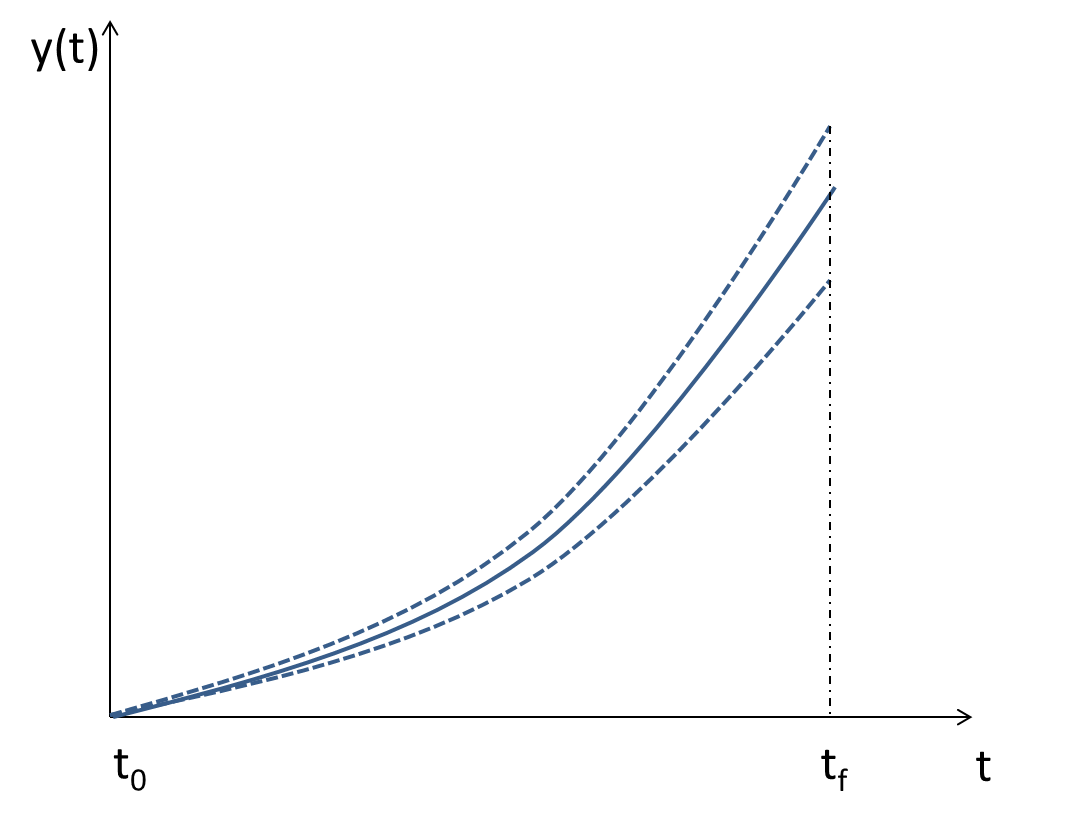
Figure 2.1: Shooting method representation (adapted from [9]). The solid line represents the solution and the dashed lines are related to the shootings

Despite its simplicity, from a practical standpoint, the shooting method is used only when the problem has a small number of variables. This method has a major disadvantage: a small change in the initial condition can produce a very large change in the final conditions. In order to overcome the numerical difficulties of the simple method, the multiple shooting method is presented.

Multiple shooting method

In a multiple shooting method, the time-interval $[t_{0},t_{f}]$ is divided into $M-1$ subintervals. Then is applied over each subinterval $[t_{i},t_{i+1}]$ with the initial values of the differential equations in the interior intervals being unknown that need to be determined. In order to enforce continuity, the following conditions are enforced at the interface of each subinterval:

$$y(t_{i}^{-})-y(t_{i}^{+})=0.$$

A scheme of the multiple shooting method is shown in Figure 2.2.

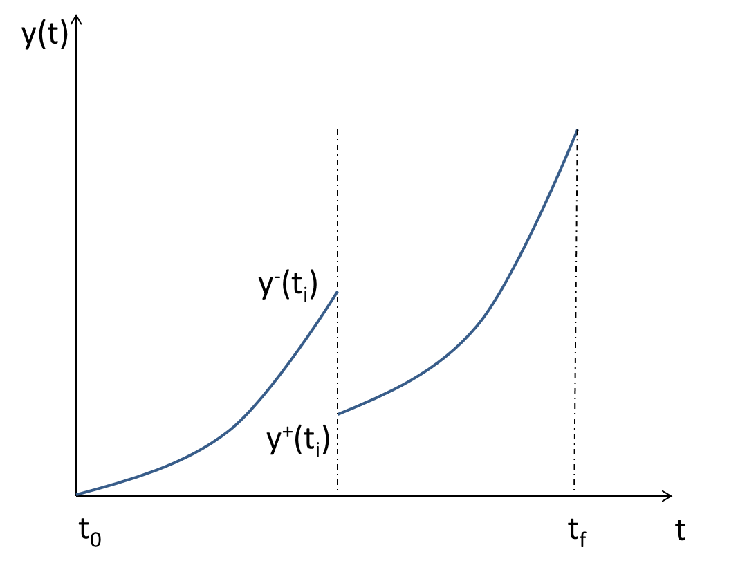
Figure 2.2: Multiple shooting method representation (adapted from [9])

With the multiple shooting approach the problem size is increased: additional variables and constraints are introduced for each shooting segment. In particular, the number of nonlinear variables and constraints for a multiple shooting application is $n=n_{y}(M-1)$, where $n_{y}$ is the number of dynamic variables $y$ and $M-1$ is the number of segments [9].

Both shooting and multiple shooting methods require a good guess for initial conditions and the propagation of the shoots for problem of high dimension is not feasible. For this reason, other methods can be implemented, using initial value problems.

The numerical solution of the IVP is fundamental to most optimal control methods. The problem can stand as follows: compute the value of $y(t_{f})$ for some value of $t<t_{f}$ that satisfies (2.1) with the known initial value $y(t_{0})=y_{0}$.

Numerical methods for solving the ODE IVP are relatively mature in comparison to other fields in Optimal Control. It will be considered two methods: single-step and multiple-step methods. In both, the solution of the differential system at each step $t_{k}$ is sequentially obtained using current and/or previous information about the solution. In both cases, it is assumed that the time $t=nh$ moves ahead in uniform steps of length $h$ [9, 51].

Euler scheme

The most common single-step method is Euler method. In this discretization scheme, if a differential equation is written like $\dot{x}=f(x(t),t)$, is possible to make a convenient approximation of this:

$$x_{n+1}\simeq x_{n}+hf(x(t_{n}),t_{n}).$$

This approximation $x_{n+1}$ of $x(t)$ at the point $t_{n+1}$ has an error of order $h^{2}$. Clearly, there is a trade-off between accuracy and complexity of calculation which depends heavily on the chosen value for $h$. In general, as $h$ is decreased the calculation takes longer but is more accurate.

For many higher order systems it is very difficult to make Euler approximation effective. For this reason more accurate and elaborate techniques were developed. One of these methods is the Runge-Kutta method.

Runge-Kutta scheme

A Runge-Kutta method is a multiple-step method, where the solution at time $t_{k+1}$ is obtained from a defined set of previous values $t_{j-k},\ldots,t_{k}$ and $j$ is the number of steps.

If a differential equation is written like $\dot{x}=f(x(t),t)$, it is possible to make a convenient approximation of this, using the second order Runge-Kutta method

$$x_{n+1}\simeq x_{n}+\frac{h}{2}\left[f(x_{n}(t),t_{n})+f(x_{n+1},t_{n+1})\right],$$

or the fourth order Runge-Kutta method

$$x_{n+1}\simeq x_{n}+\frac{h}{6}\left(k_{1}+2k_{2}+2k_{3}+k4\right)$$

where

$$k_{1}=f\left(x(t),t\right)$$

This approximation $x_{n+1}$ of $x(t)$ at the point $t_{n+1}$ has an error depending on $h^{3}$ and $h^{5}$, for the Runge-Kutta methods of second and fourth order, respectively.

Numerical methods for solving OC problems date back to the 1950s with Bellman investigation. From that time to present, the complexity of methods and corresponding complexity and variety of applications has substantially increased [108].

There are two major classes of numerical methods for solving OC problems: indirect methods and direct methods. The first ones, indirectly solve the problem by converting the optimal control problem to a boundary-value problem, using the PMP. On the other hand, in a direct method, the optimal solution is found by transcribing an infinite-dimensional optimization problem to a finite-dimensional optimization problem.

2.2 Indirect methods

In an indirect method, the PMP is used to determine the first-order optimality conditions of the original OC problem. The indirect approach leads to a multiple-point boundary-value problem that is solved to determine candidate optimal trajectories called extremals.

For an indirect method it is necessary to explicitly get the adjoint equations, the control equations and all the transversality conditions, if there exist. Notice that there is no correlation between the method used to solve the problem and its formulation: one may consider applying a multiple shooting method solution technique to either an indirect or a direct formulation. In the following subsection a numerical approach using the indirect method is presented.

Backward-Forward sweep method

This method is described in a recent book by Lenhart and Workman [81] and it is known as forward–backward sweep method. The process begins with an initial guess on the control variable. Then, the state equations are simultaneously solved forward in time and the adjoint equations are solved backward in time. The control is updated by inserting the new values of states and adjoints into its characterization, and the process is repeated until convergence occurs.

Considering $\vec{x}=(x_{1},\ldots,x_{N}+1)$ and $\vec{\lambda}=(\lambda_{1},\ldots,\lambda_{N}+1)$ the vector approximations for the state and the adjoint. The main idea of the algorithm is described as follows:

Step 1.

Make an initial guess for $\vec{u}$ over the interval ($\vec{u}\equiv 0$ is almost always sufficient);

Step 2.

Using the initial condition $x_{1}=x(t_{0})=a$ and the values for $\vec{u}$, solve $\vec{x}$ forward in time according to its differential equation in the optimality system;

Step 3.

Using the transversality condition $\lambda_{N+1}=\lambda(t_{f})=0$ and the values for $\vec{u}$ and $\vec{x}$, solve $\vec{\lambda}$ backward in time according to its differential equation in the optimality system;

Step 4.

Update $\vec{u}$ by entering the new $\vec{x}$ and $\vec{\lambda}$ values into the characterization of the optimal control;

Step 5.

Verify convergence: if the variables are sufficiently close to the corresponding in the previous iteration, then output the current values as solutions, else return to Step 2.

For Steps 2 and 3, Lenhart and Workman used for the state and adjoint systems the Runge-Kutta fourth order procedure to make the discretization process.

On the other hand, Wang [136], applied the same philosophy but solving the differential equations with the solver ode45 for Matlab. This solver is based on an explicit Runge-Kutta (4,5) formula, the Dormand-Prince pair. That means the numerical solver ode45 combines a fourth and a fifth order methods, both of which are similar to the classical fourth order Runge-Kutta method discussed above. These vary the step size, choosing it at each step an attempt to achieve the desired accuracy. Therefore, the solver ode45 is suitable for a wide variety of initial value problems in practical applications. In general, ode45 is the best method to apply as a first attempt for most problems [70].

Example 4.

Let consider the open problem defined in Chapter 1 (Example 3) about rubella disease. With $\vec{x}(t)=\left(x_{1}(t),x_{2}(t),x_{3}(t),x_{4}(t)\right)$ and $\vec{\lambda}(t)=\left(\lambda_{1}(t),\lambda_{2}(t),\lambda_{3}(t),\lambda_{4}(t)\right)$, the Hamiltonian of this problem can be written as

$$H(t,\vec{x}(t),u(t),\vec{\lambda}(t))=$$

Using the PMP the optimal control problem can be studied with the state variables

$$\dot{x}_{1}=b-b(px_{2}+qx_{2})-bx_{1}-\beta x_{1}x_{3}-ux_{1}$$

with initial conditions $x_{1}(0)=0.0555$, $x_{2}(0)=0.0003$, $x_{3}(0)=0.0004$ and $x_{4}(0)=1$ and the adjoint variables:

$$\dot{\lambda}_{1}=\lambda_{1}(b+u+\beta x_{3})-\lambda_{2}\beta x_{3}$$

with transversality conditions $\lambda_{i}(3)=0$, $i=1,\ldots,4$.

The optimal control is

$u^{*}=\left\{\begin{array}[]{lll}0&if&\frac{\partial H}{\partial u}<0\\ \frac{\lambda_{1}x_{1}}{2}&if&\frac{\partial H}{\partial u}=0\\ 0.9&if&\frac{\partial H}{\partial u}>0\end{array}\right.$

Here it is only presented the main part of the code using the backward-forward sweep method with fourth order Runge-Kutta. The completed one can be found in the website [110].

for i = 1:M
    m11 = b-b*(p*x2(i)+q*x3(i))-b*x1(i)-beta*x1(i)*x3(i)-u(i)*x1(i);
    m12 = b*p*x2(i)+beta*x1(i)*x3(i)-(e+b)*x2(i);
    m13 = e*x2(i)-(g+b)*x3(i);
    m14 = b-b*x4(i);

    m21 = b-b*(p*(x2(i)+h2*m12)+q*(x3(i)+h2*m13))-b*(x1(i)+h2*m11)-...
        beta*(x1(i)+h2*m11)*(x3(i)+h2*m13)-(0.5*(u(i) + u(i+1)))*(x1(i)+h2*m11);
    m22 = b*p*(x2(i)+h2*m12)+beta*(x1(i)+h2*m11)*(x3(i)+h2*m13)-(e+b)*(x2(i)+h2*m12);
    m23 = e*(x2(i)+h2*m12)-(g+b)*(x3(i)+h2*m13);
    m24 = b-b*(x4(i)+h2*m14);

    m31 = b-b*(p*(x2(i)+h2*m22)+q*(x3(i)+h2*m23))-b*(x1(i)+h2*m21)-...
        beta*(x1(i)+h2*m21)*(x3(i)+h2*m23)-(0.5*(u(i) + u(i+1)))*(x1(i)+h2*m21);
    m32 = b*p*(x2(i)+h2*m22)+beta*(x1(i)+h2*m21)*(x3(i)+h2*m23)-(e+b)*(x2(i)+h2*m22);
    m33 = e*(x2(i)+h2*m22)-(g+b)*(x3(i)+h2*m23);
    m34 = b-b*(x4(i)+h2*m24);

    m41 = b-b*(p*(x2(i)+h2*m32)+q*(x3(i)+h2*m33))-b*(x1(i)+h2*m31)-...
        beta*(x1(i)+h2*m31)*(x3(i)+h2*m33)-u(i+1)*(x1(i)+h2*m31);
    m42 = b*p*(x2(i)+h2*m32)+beta*(x1(i)+h2*m31)*(x3(i)+h2*m33)-(e+b)*(x2(i)+h2*m32);
    m43 = e*(x2(i)+h2*m32)-(g+b)*(x3(i)+h2*m33);
    m44 = b-b*(x4(i)+h2*m34);

    x1(i+1) = x1(i) + (h/6)*(m11 + 2*m21 + 2*m31 + m41);
    x2(i+1) = x2(i) + (h/6)*(m12 + 2*m22 + 2*m32 + m42);
    x3(i+1) = x3(i) + (h/6)*(m13 + 2*m23 + 2*m33 + m43);
    x4(i+1) = x4(i) + (h/6)*(m14 + 2*m24 + 2*m34 + m44);
end

for i = 1:M
    j = M + 2 - i;

    n11 = lambda1(j)*(b+u(j)+beta*x3(j))-lambda2(j)*beta*x3(j);
    n12 = lambda1(j)*b*p+lambda2(j)*(e+b-p*b)-lambda3(j)*e;
    n13 = -A+lambda1(j)*(b*q+beta*x1(j))-lambda2(j)*beta*x1(j)+lambda3(j)*(g+b);
    n14 = b*lambda4(j);

    n21 = (lambda1(j) - h2*n11)*(b+u(j)+beta*(0.5*(x3(j)+x3(j-1))))-...
        (lambda2(j) - h2*n12)*beta*(0.5*(x3(j)+x3(j-1)));
    n22 = (lambda1(j) - h2*n11)*b*p+(lambda2(j) - h2*n12)*(e+b-p*b)-(lambda3(j) - h2*n13)*e;
    n23 = -A+(lambda1(j) - h2*n11)*(b*q+beta*(0.5*(x1(j)+x1(j-1))))-...
        (lambda2(j) - h2*n12)*beta*(0.5*(x1(j)+x1(j-1)))+(lambda3(j) - h2*n13)*(g+b);
    n24 = b*(lambda4(j) - h2*n14);

    n31 = (lambda1(j) - h2*n21)*(b+u(j)+beta*(0.5*(x3(j)+x3(j-1))))-...
        (lambda2(j) - h2*n22)*beta*(0.5*(x3(j)+x3(j-1)));
    n32 = (lambda1(j) - h2*n21)*b*p+(lambda2(j) - h2*n22)*(e+b-p*b)-(lambda3(j) - h2*n23)*e;
    n33 = -A+(lambda1(j) - h2*n21)*(b*q+beta*(0.5*(x1(j)+x1(j-1))))-...
        (lambda2(j) - h2*n22)*beta*(0.5*(x1(j)+x1(j-1)))+(lambda3(j) - h2*n23)*(g+b);
    n34 = b*(lambda4(j) - h2*n24);

    n41 = (lambda1(j) - h2*n31)*(b+u(j)+beta*x3(j-1))-(lambda2(j) - h2*n32)*beta*x3(j-1);
    n42 = (lambda1(j) - h2*n31)*b*p+(lambda2(j) - h2*n32)*(e+b-p*b)-(lambda3(j) - h2*n33)*e;
    n43 = -A+(lambda1(j) - h2*n31)*(b*q+beta*x1(j-1))-...
        (lambda2(j) - h2*n32)*beta*x1(j-1)+(lambda3(j) - h2*n33)*(g+b);
    n44 = b*(lambda4(j) - h2*n34);

    lambda1(j-1) = lambda1(j) - h/6*(n11 + 2*n21 + 2*n31 + n41);
    lambda2(j-1) = lambda2(j) - h/6*(n12 + 2*n22 + 2*n32 + n42);
    lambda3(j-1) = lambda3(j) - h/6*(n13 + 2*n23 + 2*n33 + n43);
    lambda4(j-1) = lambda4(j) - h/6*(n14 + 2*n24 + 2*n34 + n44);
end
u1 = min(0.9,max(0,lambda1.*x1/2));

The optimal curves for the states variables and optimal control are shown in Figure 2.3.

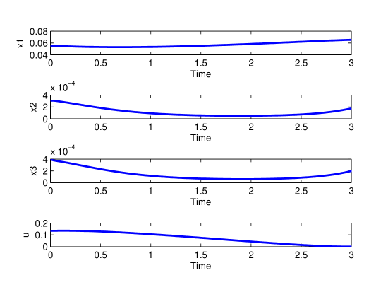
Figure 2.3: The optimal curves for rubella problem

 

There are several difficulties to overcome when an optimal control problem is solved by indirect methods. Firstly, is necessary to calculate the hamiltonian, adjoint equations, optimality condition and transversality conditions. Besides, the approach is not flexible, since each time a new problem is formulated, a new derivation is required. In contrast, a direct method does not require explicit derivation neither the necessary conditions.

Due to these practical difficulties with the indirect formulation, the main focus will be centered on the direct methods. This approach has been gaining popularity in numerical optimal control over the past three decades [9].

2.3 Direct methods

A new family of numerical methods for dynamic optimization has emerged, referred to as direct methods. This development has been driven by the industrial need to solve large-scale optimization problems and it has also been supported by the rapidly increasing computational power.

A direct method constructs a sequence of points $x_{1},x_{2},\ldots,x^{*}$ such that the objective function in minimized and typical $F(x_{1})>F(x_{2})>\cdots>F(x^{*})$. Here the state and/or control are approximated using an appropriate function approximation (e.g., polynomial approximation or piecewise constant parameterization). Simultaneously, the cost functional is approximated as a cost function. Then, the coefficients of the function approximations are treated as optimization variables and the problem is reformulated to a standard nonlinear optimization problem (NLP) in the form:

$$\underset{x,u}{min}$$

where $c_{i},i\in E$ e $c_{j},j\in I$ are the set of equality and inequality constraints, respectively.

In fact, the NLP is easier to solve than the boundary-value problem, mainly due to the sparsity of the NLP and the many well-known software programs that can handle with this feature. As a result, the range of problems that can be solved via direct methods is significantly larger than the range of problems that can be solved via indirect methods. Direct methods have become so popular these days that many people have written sophisticated software programs that employ these methods. Here we present two types of codes/packages: specific solvers for OC problems and standard NLP solvers used after a discretization process.

2.3.1 Specific Optimal Control software

OC-ODE

The OC-ODE [57], Optimal Control of Ordinary-Differential Equations, by Matthias Gerdts, is a collection of Fortran 77 routines for optimal control problems subject to ordinary differential equations. It uses an automatic direct discretization method for the transformation of the OC problem into a finite-dimensional NLP. OC-ODE includes procedures for numerical adjoint estimation and sensitivity analysis.

Example 5.

Considering the same problem (Example 3), here is the main part of the code in OC-ODE. The completed one can be found in the website [110]. The achieved solution is similar to the indirect approach, therefore we will not present it.

c     Call to OC-ODE
c      OPEN( INFO(9),FILE=’OUT’,STATUS=’UNKNOWN’)
      CALL OCODE( T, XL, XU, UL, UU, P, G, BC,
     +     TOL, TAUU, TAUX, LIW, LRW, IRES,
     +     IREALTIME, NREALTIME, HREALTIME,
     +     IADJOINT, RWADJ, LRWADJ, IWADJ, LIWADJ, .FALSE.,
     +     MERIT,IUPDATE,LENACTIVE,ACTIVE,IPARAM,PARAM,
     +     DIM,INFO,IWORK,RWORK,SOL,NVAR,IUSER,USER)
      PRINT*,’Ausgabe der Loesung: NVAR=’,NVAR
      WRITE(*,’(E30.16)’) (SOL(I),I=1,NVAR)
c      CLOSE(INFO(9))
c      READ(*,*)
      END
c-------------------------------------------------------------------------
c     Objective Function
c-------------------------------------------------------------------------
      SUBROUTINE OBJ( X0, XF, TF, P, V, IUSER, USER )
      IMPLICIT NONE
      INTEGER IUSER(*)
      DOUBLEPRECISION X0(*),XF(*),TF,P(*),V,USER(*)
      V = XF(5)
      RETURN
      END
c-------------------------------------------------------------------------
c     Differential Equation
c-------------------------------------------------------------------------
 SUBROUTINE DAE( T, X, XP, U, P, F, IFLAG, IUSER, USER )
      IMPLICIT NONE
      INTEGER IFLAG,IUSER(*)
      DOUBLEPRECISION T,X(*),XP(*),U(*),P(*),F(*),USER(*)
c     INTEGER NONE
      DOUBLEPRECISION B, E, G, P, Q, BETA, A

      B = 0.012D0
      E = 36.5D0
      G = 30.417D0
      P = 0.65D0
      Q = 0.65D0
      BETA = 527.59D0
      A = 100.0D0

      F(1) = B-B*(P*X(2)+Q*X(3))-B*X(1)-BETA*X(1)*X(3)-U(1)*X(1)
      F(2) = B*P*X(2)+BETA*X(1)*X(3)-(E+B)*X(2)
      F(3) = E*X(2)-(G+B)*X(3)
      F(4) = B-B*X(4)
      F(5) = A*X(3))+U(1)**2
      RETURN
      END

 

DOTcvp

The DOTcvp [67], Dynamic Optimization Toolbox with Vector Control Parametrization is a dynamic optimization toolbox for Matlab. The toolbox provides environment for a Fortran compiler to create the ’.dll’ files of the ODE, Jacobian, and sensitivities. However, a Fortran compiler has to be installed in a Matlab environment. The toolbox uses the control vector parametrization approach for the calculation of the optimal control profiles, giving a piecewise solution for the control. The OC problem has to be defined in Mayer form. For solving the NLP, the user can choose several deterministic solvers — Ipopt, Fmincon, FSQP — or stochastic solvers — DE, SRES.

The modified SUNDIALS tool [66] is used for solving the IVP and for the gradients and Jacobian automatic generation. Forward integration of the ODE system is ensured by CVODES, a part of SUNDIALS, which is able to perform the simultaneous or staggered sensitivity analysis too. The IVP problem can be solved with the Newton or Functional iteration module and with the Adams or BDF linear multistep method. Note that the sensitivity equations are analytically provided and the error control strategy for the sensitivity variables could be enabled. DOTcvp has a user friendly graphical interface (GUI).

Example 6.

Considering the same problem (Example 3), here is a part of the code used in DOTcvp. The completed one can be found in the website [110]. The solution, despite being piecewise continuous, follows the curve obtained by the previous programs.

% --------------------------------------------------- %
% Settings for IVP (ODEs, sensitivities):
% --------------------------------------------------- %
data.odes.Def_FORTRAN     = {’’}; %this option is needed only for FORTRAN parameters definition,
                            e.g. {’double precision k10, k20, ..’}
data.odes.parameters      = {’b=0.012’,’ e=36.5’,’ g=30.417’,’ p=0.65’,’ q=0.65’,’ beta=527.59’,
                            ’ d=0’,’ phi1=0’,’phi2=0’,’A=100 ’};
data.odes.Def_MATLAB      = {’’}; %this option is needed only for MATLAB parameters definition
data.odes.res(1)          = {’b-b*(p*y(2)+q*y(3))-b*y(1)-beta*y(1)*y(3)-u(1)*y(1)’};
data.odes.res(2)          = {’b*(p*y(2)+q*phi1*y(3))+beta*y(1)*y(3)-(e+b)*y(2)’};
data.odes.res(3)          = {’b*q*phi2*y(3)+e*y(2)-(g+b)*y(3)’};
data.odes.res(4)          = {’b-b*y(4)’};
data.odes.res(5)          = {’A*y(3)+u(1)*u(1)’};
data.odes.black_box       = {’None’,’1.0’,’FunctionName’}; %[’None’|’Full’],[penalty coefficient
                            for all constraints],...
                            [a black box model function name]
data.odes.ic              = [0.0555 0.0003 0.0004 1 0];
data.odes.NUMs            = size(data.odes.res,2); %number of state variables (y)
data.odes.t0              = 0.0; %initial time
data.odes.tf              = 3; %final time
data.odes.NonlinearSolver = ’Newton’; %[’Newton’|’Functional’] /Newton for stiff problems;
                            Functional for non-stiff problems
data.odes.LinearSolver    = ’Dense’; %direct [’Dense’|’Diag’|’Band’]; iterative
                            [’GMRES’|’BiCGStab’|’TFQMR’] /for the Newton NLS
data.odes.LMM             = ’Adams’; %[’Adams’|’BDF’] /Adams for non-stiff problems;
                            BDF for stiff problems
data.odes.MaxNumStep      = 500; %maximum number of steps
data.odes.RelTol          = 1e-007; %IVP relative tolerance level
data.odes.AbsTol          = 1e-007; %IVP absolute tolerance level
data.sens.SensAbsTol      = 1e-007; %absolute tolerance for sensitivity variables
data.sens.SensMethod      = ’Staggered’; %[’Staggered’|’Staggered1’|’Simultaneous’]
data.sens.SensErrorControl= ’on’; %[’on’|’off’]
% --------------------------------------------------- %
% NLP definition:
% --------------------------------------------------- %
data.nlp.RHO              = 10; %number of time intervals
data.nlp.problem          = ’min’; %[’min’|’max’]
data.nlp.J0               = ’y(5)’; %cost function: min-max(cost function)
data.nlp.u0               = [0 ]; %initial value for control values
data.nlp.lb               = [0 ]; %lower bounds for control values
data.nlp.ub               = [0.9]; %upper bounds for control values
data.nlp.p0               = []; %initial values for time-independent parameters
data.nlp.lbp              = []; %lower bounds for time-independent parameters
data.nlp.ubp              = []; %upper bounds for time-independent parameters
data.nlp.solver           = ’IPOPT’; %[’FMINCON’|’IPOPT’|’SRES’|’DE’|’ACOMI’|’MISQP’|’MITS’]
data.nlp.SolverSettings   = ’None’; %insert the name of the file that contains settings
                            for NLP solver, if does not exist use [’None’]
data.nlp.NLPtol           = 1e-005; %NLP tolerance level
data.nlp.GradMethod       = ’FiniteDifference’; %[’SensitivityEq’|’FiniteDifference’|’None’]
data.nlp.MaxIter          = 1000; %Maximum number of iterations
data.nlp.MaxCPUTime       = 60*60*0.25; %Maximum CPU time of the optimization
                            (60*60*0.25) = 15 minutes
data.nlp.approximation    = ’PWC’; %[’PWC’|’PWL’] PWL only for: FMINCON & without the
                            free time problem
data.nlp.FreeTime         = ’off’; %[’on’|’off’] set ’on’ if free time is considered
data.nlp.t0Time           = [data.odes.tf/data.nlp.RHO]; %initial size of the time intervals
data.nlp.lbTime           = 0.01; %lower bound of the time intervals
data.nlp.ubTime           = data.odes.tf; %upper bound of the time intervals
data.nlp.NUMc             = size(data.nlp.u0,2); %number of control variables (u)
data.nlp.NUMi             = 0; %number of integer variables (u) taken from the last
                            control variables,
if not equal to 0 you need to use some MINLP solver [’ACOMI’|’MISQP’|’MITS’]
data.nlp.NUMp             = size(data.nlp.p0,2); %number of time-independent parameters (p)

With the GUI interface this method was the preferred to be tested, due to its simple way to implement the code.

 

Muscod-II

In NEOS [98] platform there is a large set of software packages. NEOS is considered as the state of the art in optimization. One recent solver is Muscod-II [79] (Multiple Shooting CODe for Optimal Control) for the solution of mixed integer nonlinear ODE or DAE constrained optimal control problems in an extended AMPL format.

AMPL [55] is a modelling language for mathematical programming and was created by Fourer, Gay and Kernighan. The modelling languages organize and automate the tasks of modelling, which can handle a large volume of data and, moreover, can be used in machines and independent solvers, allowing the user to concentrate on the model instead of the methodology to reach solution. However, the AMPL modelling language itself does not allow the formulation of differential equations. Hence, the TACO Toolkit has been designed to implement a small set of extensions for easy and convenient modeling of optimal control problems in AMPL, without the need for explicit encoding of discretization schemes. Both the TACO Toolkit and the NEOS interface to Muscod-II are still under development.

Probably for this reason, the Example 3 could not be solved by this software which crashed after some runs. Anyway, we opted to also put the code, for the same example that is being used, to show the differences of modelling language used in each program.

Example 7.

include OptimalControl.mod;
var t ;ΨΨΨΨΨΨΨΨΨ
var x1, >=0 <=1;ΨΨ
var x2, >=0 <=1;
var x3, >=0 <=1;
var x4, >=0 <=1;ΨΨ
var u >=0, <=0.9 suffix type "u0";

minimize
cost: integral (A*x3+u^2,3);Ψ

subject to
Ψc1: diff(x1,t) = b-b*(p*x2+q*x3)-b*x1-beta*x1*x3-u*x1;
Ψc2: diff(x2,t) = b*p*x2+beta*x1*x3-(e+b)*x2;
Ψc3: diff(x3,t) = e*x2-(g+b)*x3;
Ψc4: diff(x4,t) = b-b*x4;

 

2.3.2 Nonlinear Optimization software

The three nonlinear optimization software packages presented here, were used through the NEOS platform with codes formulated in AMPL.

Ipopt

The Ipopt [135], Interior Point OPTimizer, is a software package for large-scale nonlinear optimization. It is written in Fortran and C. Ipopt implements a primal-dual interior point method and uses a line search strategy based on filter method. Ipopt can be used from various modeling environments.

Ipopt is designed to exploit 1st and 2nd derivative information if provided, usually via automatic differentiation routines in modeling environments such as AMPL. If no Hessians are provided, Ipopt will approximate them using a quasi-Newton methods, specifically a BFGS update.

Example 8.

Continuing with Example 3 the AMPL code is shown for Ipopt. The Euler discretization was the selected. Indeed, this code can also be implemented in other nonlinear software packages available in NEOS platform, reason why the code for the next two software packages will not be shown. The full version can be found on the website [110].

#### OBJECTIVE FUNCTION ###
minimize cost: fc[N];

#### CONSTRAINTS ###
subject to
Ψi1: x1[0] = x1_0;
Ψi2: x2[0] = x2_0;
Ψi3: x3[0] = x3_0;
Ψi4: x4[0] = x4_0;
Ψi5: fc[0] = fc_0;
Ψ
Ψf1 {i in 0..N-1}: x1[i+1] = x1[i] + (tf/N)*(b-b*(p*x2[i]+q*x3[i])-b*x1[i]
                                -beta*x1[i]*x3[i]-u[i]*x1[i]);
Ψf2 {i in 0..N-1}: x2[i+1] = x2[i] + (tf/N)*(b*p*x2[i]+beta*x1[i]*x3[i]-(e+b)*x2[i]);
Ψf3 {i in 0..N-1}: x3[i+1] = x3[i] + (tf/N)*(e*x2[i]-(g+b)*x3[i]);
Ψf4 {i in 0..N-1}: x4[i+1] = x4[i] + (tf/N)*(b-b*x4[i]);
Ψf5 {i in 0..N-1}: fc[i+1] = fc[i] + (tf/N)*(A*x3[i]+u[i]^2);

 

Knitro

Knitro [19], short for “Nonlinear Interior point Trust Region Optimization”, was created primarily by Richard Waltz, Jorge Nocedal, Todd Plantenga and Richard Byrd. It was introduced in 2001 as a derivative of academic research at Northwestern, and has undergone continual improvement since then.

Knitro is also a software for solving large scale mathematical optimization problems based mainly on the two Interior Point (IP) methods and one active set algorithm. Knitro is specialized for nonlinear optimization, but also solves linear programming problems, quadratic programming problems, and systems of nonlinear equations. The unknowns in these problems must be continuous variables in continuous functions; however, functions can be convex or nonconvex. The code also provides a multistart option for promoting the computation of the global minimum. This software was tested through the NEOS platform.

Snopt

Snopt [58], by Philip Gill, Walter Murray and Michael Saunders, is a software package for solving large-scale optimization problems (linear and nonlinear programs). It is specially effective for nonlinear problems whose functions and gradients are expensive to evaluate. The functions should be smooth but do not need to be convex. Snopt is implemented in Fortran 77 and distributed as source code. It uses the SQP (Sequential Quadratic Programming) philosophy, with an augmented Lagrangian approach combining a trust region approach adapted to handle the bound constraints. Snopt is also available in NEOS platform.

Choosing a method for solving an OC problem depends largely on the type of problem to be solved and the amount of time that can be invested in coding. An indirect shooting method has the advantage of being simple to understand and produces highly accurate solutions when it converges [108]. The accuracy and robustness of a direct method is highly dependent upon the method used. Nevertheless, it is easier to formulate highly complex problems in a direct way and can be used standard NLP solvers as an extra advantage. This last feature has the benefit of converging with poor initial guesses and being extremely computationally efficient since most of the solvers exploit the sparsity of the derivatives in the constraints and objective function.

In the next chapter the basic concepts from epidemiology are provided, in order to formulate/implement more complex OC problems in the health area.

Chapter 3 Epidemiological models

In this chapter, the simplest epidemiologic models composed by mutually exclusive compartments are introduced. Based on the models SIS (susceptible–infected–susceptible) and SIR (susceptible–infected–recovered), other models are presented introducing new issues related to maternal immunity or the latent period, fitting the features to distinct diseases. Illustrative examples are presented, with diseases that can be described by each model. The basic reproduction number is calculated and presented as a threshold value for the eradication or the persistence of the disease in a population.

 

In the 14th century, occurred one of most famous epidemic events: the Black Death. It killed approximately one third of the European population. From 1918-19, twenty to forty percent of the world’s population suffered from the Spanish Flu, the most severe pandemic in history. In 1978, the United Nations promoted an ambitious agreement between the countries forecasting that in the year 2000 infectious diseases would be eradicated. This conjecture failed, mainly due to the assumption that the microorganisms were biologically stationary and consequently they were not modified and became resistant to the medicines. Besides, the improvements in the transportation allowing for a faster movement of individuals and the population growing especially in developing countries, led to the appearance of new diseases and the resurgence of old ones in distinct places. Nowadays, AIDS is the most scrutinized. In 2007 there were an estimated 33.2 million sufferers worldwide, and 2.1 million deaths with over three quarters of these occurring in sub-Saharan Africa [93].

Epidemiology — the study of patterns of diseases including those which are non-communicable of infections in population — has become more relevant and indispensable in the development of new models and explanations for the outbreaks, namely due to their propagation and causes. In epidemiology, an infection is said to be endemic in a population when it is maintained in the population without the need for external inputs. An epidemic occurs when new cases of a certain disease appears, in a given human population during a given period, and then essentially disappears.

There are several types of diseases, depending on their type of transmission mechanism, of which stand out:

• bacteria, which do not confer immunity against the reinfection and frequently produce harmful toxins to the host; in case of infection, the antibiotics are usually efficient (examples: tuberculosis, meningitis, gonorrhea, syphilis, tetanus);

• viral agents, that confer immunity against reinfection; here the antibiotics do not produce effects and usually it is hoped that the immune system of the host responds to an infection by the virus or it will be necessary to take antiviral drugs that retard the multiplication of the virus (examples influenza, chicken pox, measles, rubella, mumps, HIV / AIDS, smallpox);

• vectors, that are usually mosquitoes or ticks and are infected by humans and then transmit the disease to other humans (examples: malaria, yellow fever, dengue, chikungunya).

The transmission can happen in a direct or indirect way. The direct transmission of a disease can happen by physical proximity (such as sneezing, coughing, kissing, sexual contact) or even by a specific parasite that penetrates the host through ingestion or the skin. The indirect transmission involves the vectors that are intermediaries or carriers of the infection.

In most of the cases, the direct and indirect transmission of the disease happens between the member that coexists in the host population; this is called the horizontal transmission. When the direct transmission occurs from one ascendent to a descendent not yet born (egg or embryo) it is said that vertical transmission happens [76].

When formulating a model for a particular disease, we should make a trade-off between simple models — that omit several details and generally are used for specific situations in a short time, but have the disadvantage of possibly being naive and unrealistic — and more complex models, with more details and more realistic, but generally more difficult to solve or could contain parameters which their estimates cannot be obtained.

Choosing the most appropriated model depends on the precision or generality required, the available data, and the time frame in which the results are needed. By definition, all models are “wrong”, in the sense that even the most complex will make some simplifying assumptions. It is, therefore, difficult to definitively express which model is right, though naturally we are interested in developing models that capture the essential features of a system. The art of epidemiological modelling is to make suitable choices in the model formulation making it as simple as possible and yet suitable for the question being considered [65].

3.1 Basic Terminology

Mathematical models are a simplified representation of how an infection spreads across a population over time, and generally come in two forms: stochastic and deterministic models. The first ones, employ randomness, with variables being described by probability distributions. Deterministic models split the population into subclasses, and an ODE with respect to time is formulated for each. The state variable are determined using parameters and initial conditions. The main focus in this chapter will be the deterministic models, neglecting the others.

Most epidemic models are based on dividing the population into a small number of compartments. Each containing individuals that are identical in terms of their status with respect to the disease in question. Here are some of the main compartments that a model can contain.

• Passive immune ($M$): is composed by newborns that are temporary passively immune due to antibodies transferred by their mothers;

• Susceptible ($S$): is the class of individuals who are susceptible to infection; this can include the passively immune once they lose their immunity or, more commonly, any newborn infant whose mother has never been infected and therefore has not passed on any immunity;

• Exposed or Latent ($E$): compartment referred to the individuals that despite infected, do not exhibit obvious signs of infection and the abundance of the pathogen may be too low to allow further transmission;

• Infected ($I$): in this class, the level of parasite is sufficiently large within the host and there is potential in transmitting the infection to other susceptible individuals;

• Recovered or Resistant ($R$): includes all individuals who have been infected and have recovered.

The choice of which compartments to include in a model depends on the characteristics of the particular disease being modelled and the purpose of the model. The exposed compartment is sometimes neglected, when the latent period is considered very short. Besides, the compartment of the recovered individuals cannot always be considered since there are diseases where the host has never became resistent. Acronyms for epidemiology models are often based on the flow patterns between the compartments such as MSEIR, MSEIRS, SEIR, SEIRS, SIR, SIRS, SEI, SEIS, SI, SIS.

3.2 Threshold Values

There are three commonly used threshold values in epidemiology: $\mathcal{R}_{0}$, $\sigma$ and $R$. The most common and probably the most important is the basic reproduction number [61, 64, 65].

Definition 8 (Basic reproduction number).

The basic reproduction number, denoted by $\mathcal{R}_{0}$, is defined as the average number of secondary infections that occurs when one infective is introduced into a completely susceptible population.

This threshold, $\mathcal{R}_{0}$, is a famous result due to Kermack and McKendrick [77] and is referred to as the “threshold phenomenon”, giving a borderline between a persistence or a disease death. $\mathcal{R}_{0}$ it is also called the basic reproduction ratio or basic reproductive rate.

Definition 9 (Contact number).

The contact number, $\sigma$ is the average number of adequate contacts of a typical infective during the infectious period.

An adequate contact is one that is sufficient for transmission, if the individual contacted by the susceptible is an infective. It is implicitly assumed that the infected outsider is in the host population for the entire infectious period and mixes with the host population in exactly the same way that a population native would mix.

Definition 10 (Replacement number).

The replacement number, $R$, is the average number of secondary infections produced by a typical infective during the entire period of infectiousness.

Note that the replacement number $R$ changes as a function of time $t$ as the disease evolves after the initial invasion.

These three quantities $\mathcal{R}_{0}$, $\sigma$ and $R$ are all equal at the beginning of the spreading of an infectious disease when the entire population (except the infective invader) is susceptible. $\mathcal{R}_{0}$ is only defined at the time of invasion, whereas $\sigma$ and $R$ are defined at all times.

The replacement number $R$ is the actual number of secondary cases from a typical infective, so that after the infection has invaded a population and everyone is no longer susceptible, $R$ is always less than the basic reproduction number $\mathcal{R}_{0}$. Also after the invasion, the susceptible fraction is less than one, and as such not all adequate contacts result in a new case. Thus the replacement number $R$ is always less than the contact number $\sigma$ after the invasion [64]. Combining these results leads to

$$\mathcal{R}_{0}\geq\sigma\geq R.$$

Note that $\mathcal{R}_{0}=\sigma$ for most models, and $\sigma>R$ after the invasion for all models.

For the models throughout this study the basic reproduction number, $\mathcal{R}_{0}$, will be applied. When

$$\mathcal{R}_{0}<1$$

the disease cannot invade the population and the infection will die out over a period of time. The amount of time this will take generally depends on how small $\mathcal{R}_{0}$ is. When

$$\mathcal{R}_{0}>1$$

invasion is possible and infection can spread through the population. Generally, the larger the value of $\mathcal{R}_{0}$ the more severe, and possibly widespread, the epidemic will be [42].

In Table 3.1 are some example diseases with their estimated basic reproduction number. Due to differences in demographic rates, rural-urban gradients, and contact structure, different human populations may be associated with different values of $\mathcal{R}_{0}$ for the same disease [7].

Infectious disease	Estimated $\mathcal{R}_{0}$
Influenza	3-4
Foot and mouth disease	3.5-4.5
Smallpox	3.5-6
Rubella	6-7
Dengue	1.3-11.6
Chickenpox	10-12
Measles	16-18
Whooping Cough	16-18

Table 3.1: Estimated $\mathcal{R}_{0}$ for some infectious diseases [6, 76, 100]

In the next section some of the epidemiologic models will be presented.

3.3 The SIS model

Numerous infectious diseases confer no long-lasting immunity. The SIS models are suitable for some bacterial agent diseases like meningitis, sexually transmitted diseases such as gonorrhea and for protozoan agent diseases where malaria and the sleeping sickness are good examples. For these diseases, an individual can be infected multiple times throughout their lives, with no apparent immunity. Here, recovery from infection is followed by an instant return to the susceptible compartment.

Throughout this chapter we will consider that population is constant, neglecting the tourism and immigration factors. Also it is considered that the population is homogeneously mixed, which means that every individual interacts with another at the same level and therefore all individuals have the same risk of contracting the disease.

The number of individuals in each compartment must be integer, but if the population size $N$ is sufficiently large, it is possible to treat $S$ and $I$ as continuous variables. Calculating the proportion of these compartments, varying from 0 to 1, it is considered that the total population is constant over time, i.e., $1=S+I$. The compartment changes are expressed by a system of differential equations.

The SIS model can be mathematically represented as follows.

Definition 11 (SIS model).

The SIS model can be formulated as

$$\dfrac{dS}{dt}=\gamma I-\beta SI$$

(3.1)

subject to initial conditions $S(0)>0$ and $I(0)\geq 0$.

It is considered $\beta$ the transmission rate (per capita) and $\gamma$ the recovery rate, so the mean infectious period is $1/\gamma$.

Figure 3.1 shows the epidemiological scheme of this model. Each arrow pointing towards the inside of the compartment represents a positive term in the differential equation, and the opposite direction introduces a negative term.

Figure 3.1: The SIS schematic model

The vital dynamics (births and deaths) were not considered, but a similar model can be constructed with these effects [65]. Despite this lack of susceptible births, the disease can still persist because the recovery of infected individuals replenishes the susceptible class and will guarantee the long-term persistence of the disease.

Remark 5.

The SI model is a particular case of the SIS model when the recovery rate ($\gamma$) is null.

A new infected individual is expected to infect another at a transmission rate $\beta$, during $\frac{1}{\gamma}$ that is the infectious period, so the expected basic reproduction number is

$$\mathcal{R}_{0}=\frac{\beta}{\gamma}.$$

Example 9.

Trachoma is an infectious disease causing a characteristic roughening of the inner surface of the eyelids. Also called granular conjunctivitis or Egyptian ophthalmia, it is the leading cause of infectious blindness in the world. Adapting a model from [109], and using $\beta=0.047$ as transmission rate and the recovery rate $\gamma=0.017$, we have the basic reproduction number $\mathcal{R}_{0}$ approximately 2.76 and the following representation of the state variables (Figure 3.2).

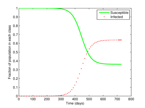
Figure 3.2: Deterministic SIS model for trachoma disease, using as initial conditions $S(0)=1-10^{-6}$ and $I(0)=10^{-6}$

 

3.4 The SIR model

The SIR model was initially studied in depth by Kermack and McKendrick and categorizes hosts within a population as Susceptible, Infected and Recovered [77]. It captures the dynamics of acute infections that confers lifelong immunity once recovered. Diseases where individuals acquire permanent immunity, and for which this model may be applied, include measles, smallpox, chickenpox, mumps, typhoid fever and diphtheria.

Once again we will consider the total population size constant, i.e., $1=S+I+R$. Two cases will be studied, distinguished by the inclusion or exclusion of demographic factors.

3.4.1 The SIR model without demography

Having compartmentalized the population, we now need a set of equations that specify how the sizes of compartments change over time.

Definition 12 (SIR model without demography).

The SIR model, excluding births and deaths, can be defined as

$$\frac{dS}{dt}=-\beta SI$$

(3.2)

subject to initial conditions $S(0)>0$, $I(0)\geq 0$ and $R(0)\geq 0$.

In addition, the transmission rate, per capita, is $\beta$ and the recovery rate is $\gamma$. Figure 3.3 presents a epidemiological scheme for this model.

Figure 3.3: The SIR schematic model without demography effects

Since population is constant and as $R$ does not appear in the first two differential equations, most of the times the last equation is omitted, indeed, $R(t)=1-S(t)-I(t)$. By assuming equations from (3.2) is possible to notice that

$$\frac{dS}{dt}+\frac{dI}{dt}+\frac{dR}{dt}=0.$$

Then a newly introduced infected individual can be expected to infect other people at the rate $\beta$ during the expected infectious period $1/\gamma$. Thus, this first infective individual can be expected to infect

$$\mathcal{R}_{0}=\frac{\beta}{\gamma}.$$

Example 10.

Consider an epidemic of influenza in a British boarding school in early 1978 [76]. Three boys were reported to the school infirmary with the typical symptoms of influenza. Over the next few days, a very large fraction of the 763 boys in the school had contact with the infection. Within two weeks, the infection had become extinguished. The best fit parameters yield an estimated active infectious period of $1/\gamma=2.2$ days and a mean transmission rate $\beta=1.66$ per day. Therefore, the estimated $\mathcal{R}_{0}$ is 3.652. Figure 3.4 represents the dynamics of the three state variables.

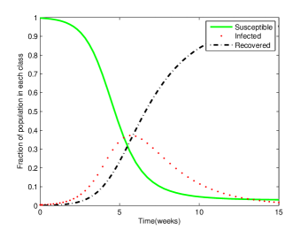
Figure 3.4: The time-evolution of influenza over 15 days

 

It was presented a SIR model given the assumption that the time scale of disease spread was sufficiently fast that births and deaths can be neglected. In the next subsection we explore the long-term persistence and endemic dynamics of an infectious disease.

3.4.2 The SIR model with demography

The simplest and most common way of introducing demography into the SIR model is to assume there is a natural host lifespan, $1/\mu$ years. Then, the rate at which individuals, at any epidemiological compartment, suffer natural mortality is given by $\mu$. It is important to emphasize that this factor is independent of the disease and is not intended to reflect the pathogenicity of the infectious agent. Historically, it has been assumed that $\mu$ also represents the population’s crude birth rate, thus ensuring that total population size does not change through time, or in other words, $\frac{dS}{dt}+\frac{dI}{dt}+\frac{dR}{dt}=0$.

Putting all these assumptions together, we have a new definition.

Definition 13 (SIR model with demography).

The SIR model, including births and deaths, can be defined as

$$\frac{dS}{dt}=\mu-\beta SI-\mu S$$

(3.3)

with initial conditions $S(0)>0$, $I(0)\geq 0$ and $R(0)\geq 0$.

The epidemiological scheme is in Figure 3.5.

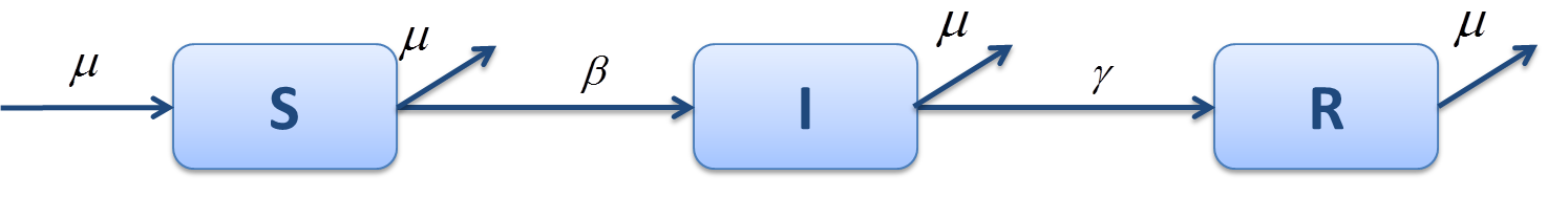
Figure 3.5: The SIR schematic model with demography effects

It is important to introduce the $\mathcal{R}_{0}$ expression for this model. The parameter $\beta$ represents the transmission rate per infective and the negative terms in the equation tell us that each individual spends an average $\frac{1}{\gamma+\mu}$ time units in this class. Therefore, if we assume the entire population is susceptible, then the average number of new infectious per infectious individual is determined by

$$\mathcal{R}_{0}=\frac{\beta}{\gamma+\mu}.$$

The inclusion of demographic dynamics may allow a disease to die out or persist in a population in the long term. For this reason it is important to explore what happens when the system is at equilibrium.

Definition 14 (Equilibrium points).

A model defined SIR has an equilibrium point, if a triple $E^{*}=\left(S^{*},I^{*},R^{*}\right)$ satisfies the following system:

$$\begin{cases}\frac{dS}{dt}=0\\ \frac{dI}{dt}=0\\ \frac{dR}{dt}=0\\ \end{cases}.$$

If the equilibrium point has the infectious component equal to zero ($I^{*}=0$), this means that the pathogen suffered extinction and $E^{*}$ is called Disease Free equilibrium (DFE).

If $I^{*}>0$ the disease persist in the population and $E^{*}$ is called Endemic Equilibrium (EE).

With some calculations and algebraic manipulations, it is possible to obtain two equilibria for the system (3.3):

DFE: $$E^{*}_{1}=(1,0,0)$$

EE:

When $\mathcal{R}_{0}<1$, each infected individual produces, on average, less than one new infected individual, and therefore, predictable that the infection will be cleared from the population. If $\mathcal{R}_{0}>1$, the pathogen is able to invade the susceptible population [61, 64]. It is possible to prove that for the Endemic Equilibrium to be stable, $\mathcal{R}_{0}$ must be greater than one, otherwise the Disease Free Equilibrium is stable. More detailed information about local and global stability of the equilibrium point can be found in [22, 74, 83, 91].

This threshold behavior is very useful, once we can determine which control measures, and at what magnitude, would be most effective in reducing $\mathcal{R}_{0}$ below one, providing important guidance for public health initiatives.

Example 11.

The SIR model below, Figure 3.6, is plotted using similar parameters and initial conditions, except the transmission rate $\beta$ (adapted from [76]).

It is shown that in case (a), using $\beta=520$, the basic reproduction number is greater than one. With demographic effects could have damped oscillations with a decreasing amplitude, in the EE direction. In case (b), with $\beta=10$, we obtain $\mathcal{R}_{0}<1$ and the system tends to go to a DFE.

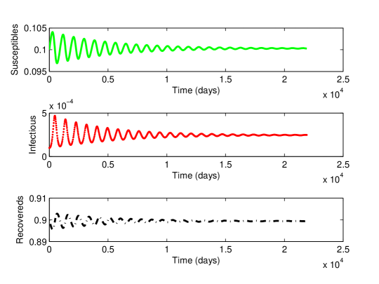
(a) $\beta=520$ per year, $1/\mu=70$ years and $1/\gamma=7$ days, giving $\mathcal{R}_{0}$ approximately 9.97

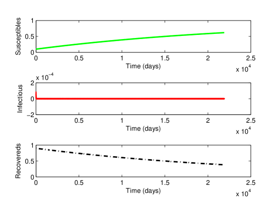
(b) $\beta=10$ per year, $1/\mu=70$ years and $1/\gamma=7$ days, giving $\mathcal{R}_{0}$ approximately 0.19

Figure 3.6: Dynamics of SIR model with distinct basic reproduction numbers

 

The next three sections present a brief description of other possible refinements of the basic models SIS and SIR.

3.5 The SEIR model

In the SEIR case, the transmission process occurs with an initial inoculation with a very small number of pathogens. Then, during a period of time the pathogen reproduces rapidly within the host, relatively unchallenged by the immune system. During this stage, pathogen abundance is too low for active transmission to other susceptible host, and yet the pathogen is present. The time in this stage is very difficult to quantify, since there is no symptomatic features of the disease. It is called the latent or exposed period. Assuming the average duration of the latent period is given by $\frac{1}{\nu}$, the SEIR model can be described as follow.

Definition 15 (SEIR model).

The SEIR model is formulated as

$$\frac{dS}{dt}=\mu-(\beta I+\mu)S$$

(3.4)

with initial conditions $S(0)>0$, $E(0)\geq 0$, $I(0)\geq 0$ and $R(0)\geq 0$.

The parameter $\beta$ and $\gamma$ were defined in the previous section. The epidemiological scheme for SEIR model is presented in Figure 3.7.

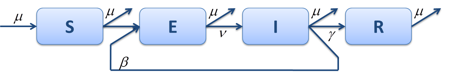
Figure 3.7: The SEIR schematic model

The expression for the basic reproduction number is

$$\mathcal{R}_{0}=\frac{\beta\nu}{(\gamma+\mu)(\nu+\mu)}.$$

This threshold is the product of the contact rate $\beta$ per unit time, the average infectious period adjusts to the population growth of $\frac{1}{\gamma+\mu}$, and the fraction $\frac{\nu}{\nu+\mu}$ of exposed people surviving the latent class $E$.

Finding steady states of the system, we obtain the following equilibrium points:

DFE: $$E^{*}_{1}=(1,0,0,0)$$

EE:

with

$$S^{*}=\frac{1}{\mathcal{R}_{0}}$$

Although the SIR and SEIR models behave similarly at equilibrium, when the parameters are suitably adapted, the SEIR model has a slower growth rate after pathogen invasion. This is due to the fact that individuals need to stay some time in the exposed class before their contribution in the disease transmission chain [76].

3.6 The MSEIR model

An infected or vaccinated mother transfers some antibodies across the placenta to her fetus, so that the newborn infant has temporary passive immunity to an infection. Since the infant can not produce new antibodies, when these passive antibodies are gone at a rate $\delta$, the baby passes from the immune state $M$ to the susceptible state $S$. Some childhood diseases have this feature. The birth rate $\mu S$ into the susceptible class of size $S$ corresponds to newborns whose mothers are susceptible, and the other newborns $\mu(1-S)$ enter passively immune class of size $M$, since their mothers were infected or had some type of immunity [65].

The transfer diagram for the MSEIR model is shown in Figure 3.8.

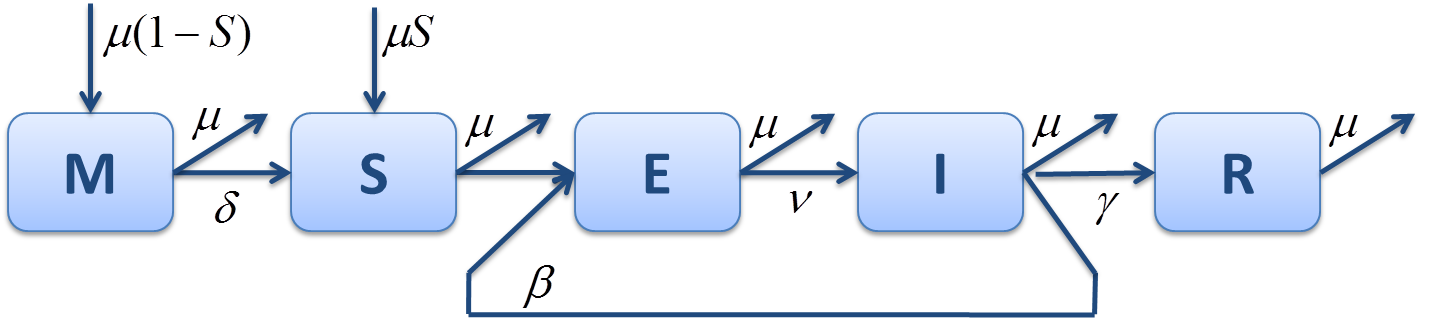
Figure 3.8: The MSEIR schematic model

The MSEIR is also composed by a system of differential equations.

Definition 16 (MSEIR model).

The SEIR model can be described as

$$\frac{dM}{dt}=\mu-(\delta+\mu)M$$

(3.5)

with initial conditions $M(0)\geq 0$, $S(0)>0$, $E(0)\geq 0$, $I(0)\geq 0$ and $R(0)\geq 0$.

Thus, the basic reproduction number is equal to previous model $SEIR$, once the $M$ compartment does not affect the transmission chain of the disease:

$$\mathcal{R}_{0}=\frac{\beta\nu}{(\gamma+\mu)(\nu+\mu)}.$$

The equations (3.5) always have a DFE given by

$$E_{1}^{*}=(0,1,0,0,0).$$

If $\mathcal{R}_{0}>1$, there is also a unique EE given by $E_{2}^{*}=\left(M^{*},S^{*},E^{*},I^{*},R^{*}\right)$, where

$$M^{*}=\frac{\mu}{\delta+\mu}\left(1-\frac{1}{\mathcal{R}_{0}}\right)$$

There are several models with different epidemiological states, such as MSEIRS, SEIRS, SEI, SI, SIRS, depending on the specific features and the level of detail that is wished to introduce in the model. These models are similar to the previous ones presented. Other epidemiological models can be studied using more compartments such as Quarantine-Isolation ($Q$), Treatment ($T$), Carrier ($C$) or Vaccination ($V$). Besides, most of the populations can be subdivided into different groups (sex, age, health weaknesses, …), depending upon characteristics that may influence the risk of catching and/or transmitting an infection. More details and examples can be found in [4, 14, 65, 134]. Other diseases can be caught and transmitted by numerous hosts or even is required a second different population to complete the transmission cycle, such as vector borne-diseases, using double models. This last case will be explored in the second part of the thesis.

In cases that include multiple compartments of infected individuals, in which vital and epidemiological parameters depend on factors as stage of the disease, spatial position, age, behavior, multigroups, the next generation method is the more generalized approach to calculate $\mathcal{R}_{0}$.

3.7 $\mathcal{R}_{0}$ using the next generation method

The definition of $\mathcal{R}_{0}$ has more than one possible interpretation, depending on the field (ecology, demography or epidemiology) and there exist distinct methods and estimations to calculate this threshold.

The next generation method, introduced by Diekmann et al.[39], defines $\mathcal{R}_{0}$ as the spectral radius of the next generator operator. The formation of the operator involves the determination of two compartments, infected and non-infected from the model. Recent examples of this method are given in [38, 42, 61, 142].

Let us assume that there are $n$ compartments of which $m$ are infected. We defined the vector $x=(x_{1},\ldots,x_{n})^{T}$, where $x_{i}\geq 0$ denotes the number of proportion of individuals in the $i$th compartment. For clarity we sort the compartments so that the first $m$ compartments correspond to infected individuals. The distinction between infected and uninfected compartments must be determined from the epidemiological interpretation, and not by the mathematical expressions.

It is necessary to define the set

$$X_{s}=\{x\geq 0|x_{i}=0,i=1,\ldots,m\}.$$

Let $\mathcal{F}_{i}(x)$ be the rate of appearance of new infections in compartment $i$ and let $\mathcal{V}_{i}(x)=V_{i}^{-}(x)-V_{i}^{+}(x)$, where $V_{i}^{+}$ is the rate of transfer of individuals into compartment $i$ by all other means and $V_{i}^{-}$ is the rate of transfer of individuals out of the $i$th compartment.

The disease transmission model consists of nonnegative initial conditions together with the following system of equations:

$$\dot{x}_{i}=f_{i}(x)=\mathcal{F}_{i}(x)-\mathcal{V}_{i}(x)$$ (3.6)

Note that $F_{i}$ should include only infections that are newly arising, but does not include terms which describe the transfer of infectious individuals from one infected compartment to another.

Let us consider the following assumptions:

(A1)

If $x\geq 0$, then $\mathcal{F}_{i}$, $\mathcal{V}_{i}^{+}$, $\mathcal{V}_{i}^{-}\geq 0$ for $i=1,\ldots,n$.

(A2)

If $x_{i}=0$ then $\mathcal{V}_{i}^{-}=0$. In particular, if $x\in X_{s}$ then $\mathcal{V}_{i}^{-}=0$ for $i=1,\ldots,m$.

(A3)

$\mathcal{F}_{i}=0$ if $i>m$.

(A4)

If $x_{i}\in X_{s}$ then $\mathcal{F}_{i}(x)=0$ and $\mathcal{V}_{i}^{+}(x)=0$ for $i=1,\ldots,m$.

(A5)

If $\mathcal{F}(x)$ is set to zero, then all eigenvalues of $Df(x_{0})$ have negative real parts and $Df(x_{0})$ is the derivative $\left[\frac{\partial f_{i}}{\partial x_{j}}\right]$ evaluated at the DFE $x_{0}$.

Assuming that $\mathcal{F}_{i}$ and $\mathcal{V}_{i}$ meet the assumptions above, we can form the next generation matrix $FV^{-1}$ from matrices of partial derivatives of $\mathcal{F}_{i}$ and $\mathcal{V}_{i}$. Specially,

$$F=\left[\frac{\partial\mathcal{F}_{i}}{\partial x_{j}}(x_{0})\right]$$ and

where $i,j=1,\ldots,m$ and $x_{0}$ is the DFE.

The entries of $FV^{-1}$ give the rate at which infected individuals in $x_{j}$ produce new infections in $x_{i}$, times the average length of time an individual spends on a single visit to compartment $j$.

Definition 17 (Basic reproduction number using the next generator operator).

The basic reproduction number is given by

$$\mathcal{R}_{0}=\rho(FV^{-1})$$ (3.7)

where $\rho$ denotes the spectral radius (dominant eigenvalue) of the matrix $FV^{-1}$.

The following theorem states that $\mathcal{R}_{0}$ is a threshold parameter for the stability of the DFE.

Theorem 3.7.1.

Consider the disease transmission model given by (3.6) with $f(x)$ satisfying conditions (A1)–(A5). If $x_{0}$ is a DFE of the model, then $x_{0}$ is locally asymptotically stable if $\mathcal{R}_{0}<1$, but unstable if $\mathcal{R}_{0}>1$, where $\mathcal{R}_{0}$ is defined by (3.7).

Proof.

The proof of this theorem can be found in [42]. ∎

Example 12.

Consider a simple model SEIT for tuberculosis with a treated compartment (adapted from [11]). Tuberculosis, is a common, and in many cases lethal, infectious disease caused by various strains of mycobacteria. Tuberculosis typically attacks the lungs but can also affect other parts of the body. Most infections are asymptomatic and latent, but about one in ten latent infections eventually progresses to active disease which, if left untreated, kills more than 50% of those so infected.

In this model a constant population is considered where $N=S+E+I+T$. Exposed individuals progress to the infectious compartment at a rate $\nu$. The treatment rates are $r_{1}$ for exposed individuals and $r_{2}$ for infectious individuals. However only a fraction $q$ of the treatments of infectious individuals are successful. Unsuccessfully treated infectious individuals re-enter the exposed compartment ($1-q$). The dynamics are illustrated in Figure 3.9 and the differential equations are the following:

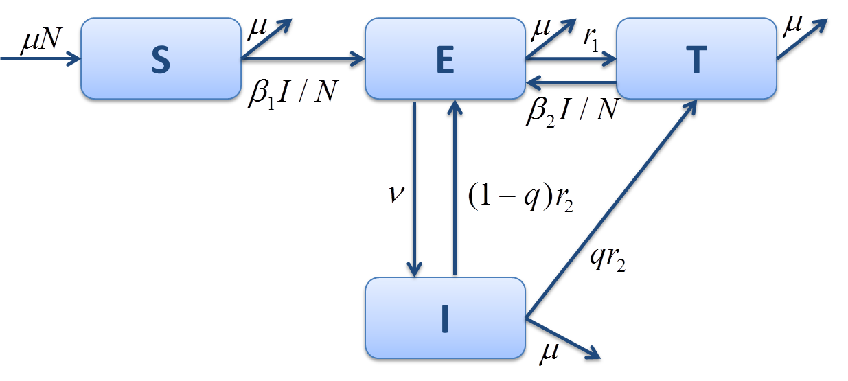
Figure 3.9: The SEIT schematic model

$$\frac{dS}{dt}=\mu N-\left(\beta_{1}\frac{I}{N}+\mu\right)S$$

A Disease Free Equilibrium is $x_{0}=(N,0,0,0)^{T}$. Note that progression from $E$ to $I$ and failure of treatment are not considered to be new infections. Thus, let only consider the infected compartments $E$ and $I$, which gives $m=2$, and we will construct the matrices $\mathcal{F}$ and $\mathcal{V}$ only related to these compartments. Let

$\mathcal{F}(x)=\left(\begin{array}[]{c}\beta_{1}\frac{IS}{N}+\beta_{2}\frac{IT}{N}\\ 0\\ \end{array}\right)$ and $\mathcal{V}(x)=\left(\begin{array}[]{c}-(1-q)r_{2}I+\left(\nu+r_{1}+\mu\right)E\\ -\nu E+\left(r_{2}+\mu\right)I\\ \end{array}\right).$

Hence

$F(x_{0})=\left(\begin{array}[]{cc}0&\beta_{1}\\ 0&0\\ \end{array}\right)$ and $V(x_{0})=\left(\begin{array}[]{cc}\nu+r_{1}+\mu&-(1-q)r_{2}\\ -\nu&r_{2}+\mu\\ \end{array}\right).$

This way,

$$\mathcal{R}_{0}=\rho(FV^{-1})=\frac{\beta_{1}\nu}{(\nu+r_{1}+\mu)(r_{2}+\mu)-\nu(1-q)r_{2}}.$$

 

Epidemiological models can be understood as a framework to explain the mechanisms of the disease procedures and test ideas to implement control measures. $\mathcal{R}_{0}$ is a key concept, used as a threshold parameter to predict where an infection will spread and how these controls can be effective.

In the second part of the thesis, the epidemiological models will be used for studying Dengue disease. Applying OC theory, the repercussions of several controls in the development of the disease will be analyzed.

Part II Original Results

Chapter 4 A first contact with the Dengue disease

During the last decades, the global prevalence of Dengue progressed dramatically. In this chapter, Dengue details are given, such as disease symptoms, transmission and epidemiological trends. An old OC model for Dengue is revisited, as a first approach to the disease. Due to the software robustness improvements and the higher computational capacity, a better solution for this problem is proposed. In order to study different discretization schemes for an OC problem, taking into account time performance and resources used, some numerical simulations are made using Euler and Runge-Kutta methods.

 

The origins of the word Dengue are not clear. Some researchers think that it is derived from the Swahili phrase “Ka-dinga pepo”, meaning “cramp-like seizure caused by an evil spirit”. The first recognized Dengue epidemics occurred almost simultaneously in Asia, Africa, and North America in the 1780s, shortly after the identification and naming of the disease in 1779 [33].

Dengue transcends international borders and can be found in tropical and subtropical regions around the world, predominantly in urban and semi-urban areas. Dengue is a disease which is now endemic in more than one hundred countries of Africa, America, Asia and the Western Pacific. In Figure 4.1 it is possible to see the areas that in 2008 have more surveillance.

Nevertheless, some studies have indicated that countries with a mild climate, such as in the Mediterranean, are at risk due to future climate conditions that may be favorable to this kind of disease [69]. In Europe there are no registered cases, but the main vector of the disease is already in the old continent and has been followed on Madeira island [5, 124]. This risk may be aggravated further due to climate changes and to the globalization, as a consequence of the huge volume of international tourism and trade [122]. Travelers play an essential role in the global epidemiology: they act as viremic travelers, carrying the disease into areas where mosquitos can transmit the infection.

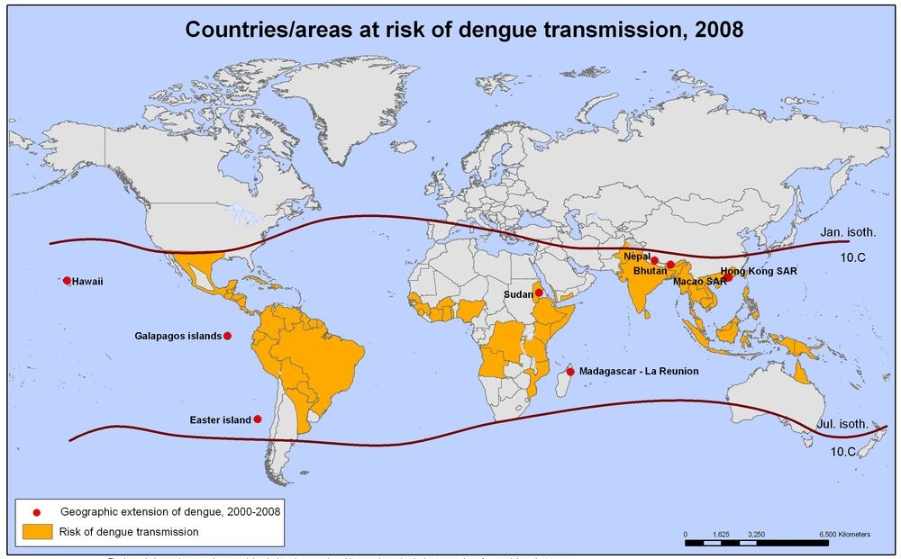
Figure 4.1: Countries/areas at risk of Dengue transmission, 2008 (Source WHO)

4.1 Background for Dengue

4.1.1 Dengue Fever and Dengue Hemorrhagic Fever

Dengue is a vector-borne disease transmitted from an infected human to a female Aedes mosquito by a bite. Then, the mosquito, that needs regular meals of blood to feed their eggs, bites a potential healthy human and transmits the disease making it a cycle.

There are two forms of Dengue: Dengue Fever (DF) and Dengue Hemorrhagic Fever (DHF). The first one is characterized by a sudden high fever without respiratory symptoms, accompanied by intense headaches, painful joints and muscles and lasts between three to seven days. Humans may only transmit the virus during the febrile stage [33]. DHF initially exhibits a similar, if more severe pathology as DF, but deviates from the classic pattern at the end of the febrile stage [54]. The hemorrhagic form has an additionally bleeding from the nose, mouth and gums or skin bruising, nausea, vomiting and fainting due to low blood pressure by fluid leakage. It usually lasts between two to three days and can lead to death [36]. Nowadays, Dengue is the mosquito-borne infection that has become a major international public health concern. According to the World Health Organization (WHO), 50 to 100 million Dengue Fever infections occur yearly, including 500000 Dengue Hemorrhagic Fever cases and 22000 deaths, mostly among children [141].

There are four distinct, but closely related, viruses that cause Dengue. The four serotypes, named DEN-1 to DEN-4, belong to the Flavivirus family, but they are antigenically distinct. Recovery from infection by one virus provides lifelong immunity against that virus but confers only partial and transient protection against subsequent infection by the other three viruses. There is good evidence that a sequential infection increases the risk of developing DHF [137].

Unfortunately, there is no specific effective treatment for Dengue. Activities, such as triage and management, are critical in determining the clinical outcome of Dengue. A rapid and efficient front-line response not only reduces the number of unnecessary hospital admissions but also saves lives.

Although up until now there is no effective and safe vaccine for Dengue, a number of candidates are undergoing various phases of clinical trials [140]. With four closely related viruses that can cause the disease, there is a need for a vaccine that would immunize against all four types to be effective. The main difficulty in the vaccine production is that there is a limited understanding of how the disease typically behaves and how the virus interacts with the immune system. Another challenge is that some studies show that some secondary Dengue infection can leave to DHF, and theoretically a vaccine could be a potential cause of severe disease if a solid immunity is not established against the four serotypes. Research to develop a vaccine is ongoing and the incentives to study the mechanism of protective immunity are gaining more support, now that the number of outbreaks around the world is increasing [33].

The spread of Dengue is attributed to the geographic expansion of the mosquitoes responsible for the disease: Aedes aegypti and Aedes albopictus [23]. Due to its higher interaction with humans and its urban behavior, the first mosquito is considered the major responsible for Dengue transmission and, our attention will be focused on it.

4.1.2 Biological notes on Aedes aegypti

Aedes aegypti, in Figure 4.2, is an insect species closely associated with humans and their dwellings, thriving in crowded cities and biting primarily during the day. Humans not only provide blood meals for mosquitoes, but also nutrients needed for them to reproduce through water-holding containers, in and around their homes. In urban areas, Aedes mosquitoes breed on water collections in artificial containers such as cans, plastic cups, used tires, broken bottles and flower pots. With increasing urbanization, crowded cities, poor sanitation and lack of hygiene, environmental conditions foster the spread of the disease that, even in the absence of fatal forms, breed significant economic and social costs (absenteeism, immobilization, debilitation and medication) [35].

The mosquito Aedes aegypti is a tropical and subtropical specie widely distributed around the world, mostly between latitudes $35^{o}$N and 35^oS, which corresponds, approximately, to a winter isotherm of 10^oC [13], as Figure 4.1 illustrates.

Figure 4.2: Mosquito Aedes aegypti

Dengue is spread only by adult females that require a blood meal for the development of their eggs, whereas male mosquitoes feed on fruit nectar and other sources of sugar. In this process the female acquire the virus while feeding on the blood of an infected person. After virus incubation from eight to twelve days (extrinsic period), an infected mosquito is capable, during probing and blood feeding, of transmitting the virus for the rest of its life to susceptible humans, and the intrinsic period for humans varies from 3 to 15 days.

The life cycle of a mosquito has four distinct stages: egg, larva, pupa and adult, as it is possible to see in Figure 4.3. In the case of Aedes aegypti, the first three stages take place in or near water whilst air is the medium for the adult stage [103]. Female mosquitoes lay their eggs, but usually do not lay them all at once: it releases them in different places, increasing the probability of new births [139].

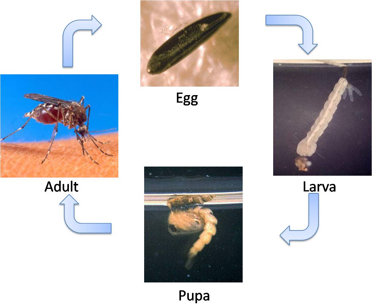
Figure 4.3: Life cycle of Aedes aegypti

The eggs of Aedes aegypti can resist to droughts and low temperatures for up to one year. Although the hatching of mature eggs may occur spontaneously at any time, this is greatly stimulated by flooding. Larvae hatch when water inundates the eggs as a result of rains or an addition of water by people. In the following days, the larvae will feed on microorganisms and particulate organic matter. When the larva has acquired enough energy and size, metamorphosis is done, changing the larva into pupa. Pupae do not feed: they just change in form until the adult body is formed. The newly formed adult emerges from the water after breaking the pupal skin. The entire life cycle, from the aquatic phase (eggs, larvae, pupae) to the adult phase, lasts from 8 to 10 days at room temperature, depending on the level of feeding [27]. The adult stage of the mosquito is considered to last an average of eleven days in an urban environment, reaching up to 30 days in laboratory environment.

Studies suggest that most female mosquitoes may spend their lifetime in or around the houses where they emerge as adults. This means that people, rather than mosquitoes, rapidly move the virus within and between communities.

Aedes aegypti is one of the most efficient vectors for arboviruses because it is highly anthropophilic, frequently bites several times before complete oogenesis [141]. The extent of Dengue transmission is determined by a wide variety of factors: the level of herd immunity in the human population to circulating virus serotype(s); virulence characteristics of the viral strain; survival, feeding behavior, and abundance of aedes aegypti; climate; and human density, distribution, and movement [121].

It is very difficult to control or eliminate aedes aegypti mosquitoes because they are highly resilient, quickly adapting to changes in the environment and they have the ability to rapidly bounce back to initial numbers after disturbances resulting from natural phenomena (e.g., droughts) or human interventions (e.g., control measures). We can safely expect that transmission thresholds will vary depending on a range of factors.

4.1.3 Measures to fight Dengue

Primary prevention of Dengue resides mainly in mosquito control. There are two primary methods: larval control and adult mosquito control, depending on the intended target [96]. Larvicide treatment is done through long-lasting chemical in order to kill larvae and preferably have WHO clearance for use in drinking water [36]. The application of adulticides can have a powerful impact on the abundance of adult mosquito vector. However, the efficacy is often constrained by the difficulty in achieving sufficiently high coverage of resting surfaces [37]. This is the most common measure. However the long term use of adulticide has several risks: the resistance of the mosquito to the product reducing its efficacy, the killing of other species that live in the same habitat and has also been linked to numerous adverse health effects including the worsening of asthma and respiratory problems.

Larvicide treatment is an effective way to control the vector larvae, together with mechanical control, which is related to educational campaigns. The mechanical control must be done by both public health officials and residents in affected area. The participation of the entire population is essential in removing still water from domestic recipients and eliminating possible breeding sites [140].

The most recent approach for fighting the disease is biological control. It is a natural process of population regulation through natural enemies. There are techniques that combine some parasites that kill partially the larval population; however there are some operational resistance, because there is lack of expertise in producing these type of parasites and there are some cultural objections in introducing something in the water for human consumption [23].

Another way of insect control is to change the reproduction process, releasing sterile insects. This technique, named as Sterile Insect Technique, consists in releasing sterile insects in natural environment, so that the result of mating produces the non-viability of the eggs, and thus can lead to drastic reduction of the specie. This way of control, shows two types of inconvenience: it is expensive to produce and release insects, and can be confronted with social objections, because an uninformed population could not correctly understand the addition of insects as a good solution [8, 47, 131].

Mathematical modeling became an interesting tool for understanding epidemiological diseases and for proposing effective strategies in fighting them. A set of mathematical models have been developed in literature to gain insights into the transmission dynamics of Dengue in a community. While Zeng and Velasco-Hérnandez [49] investigate the competitive exclusion principle in a two-strain Dengue model, Chowell et al. [26] estimates the basic reproduction number for Dengue using spatial epidemic data. In [100] the author studies the spread of Dengue thought statistical analysis, while in Tewa et al. [130] global asymptotic stability of the equilibrium of a single-strain Dengue model is established. The control of the mosquito by the introduction of a sterile insect technique is analyzed in Thomé et al. [132]. More recently, a study in disease persistence was made [88] in Brazil and Otero et al. [102] studied Dengue outbreaks. All these studies were made with the aim of providing a better understanding of the nature and dynamics of Dengue infection transmission. In the next section a temporal mathematical model that explores the dynamics between hosts (humans) and vectors (mosquitoes) is analyzed.

4.2 A first mathematical approach to Dengue epidemics

The aim of this section is to present a mathematical model to study the dynamic of the Dengue epidemics, in order to minimize the investments in disease’s control, since financial resources are always scarce. Quantitative methods are applied to the optimization of investments in the control of the epidemiologic disease, in order to obtain a maximum of benefits from a fixed amount of financial resources. The used model depends on the dynamic of the mosquito growing, but also on the efforts of public management to motivate the population to break the reproduction cycle of the mosquitoes by avoiding the accumulation of still water in open-air recipients and spraying potential zones of reproduction.

4.2.1 Mathematical model

The Dengue epidemic model described in this paper is based on the one proposed in [20]. It has four state variables and two control variables as follows.

State Variables:
$x_{1}(t):$	density of mosquitoes
$x_{2}(t):$	density of mosquitoes carrying the virus
$x_{3}(t):$	number of individuals with the disease
$x_{4}(t):$	level of popular motivation to combat mosquitoes (goodwill)

Control Variables:
$u_{1}(t):$	investments in insecticides
$u_{2}(t):$	investments in educational campaigns

To describe the model it is also necessary to introduce some parameters:

Parameters:
$\alpha_{R}:$	average reproduction rate of mosquitoes
$\alpha_{M}:$	mortality rate of mosquitoes
$\beta:$	probability of contact between non-carrier mosquitoes and infected individuals
$\eta:$	rate of treatment of infected individuals
$\mu:$	amplitude of seasonal oscillation in the reproduction rate of mosquitoes
$\rho:$	probability of individuals becoming infected
$\theta:$	fear factor, reflecting the increase in the population willingness to take actions to combat the mosquitoes as a consequence of the high prevalence of the disease in the specific social environment
$\tau:$	forgetting rate for goodwill of the target population
$\varphi:$	phase angle to adjust the peak season for mosquitoes
$\omega:$	angular frequency of the mosquitoes proliferation cycle, corresponding to a 52 weeks period
$P:$	population in the risk area (usually normalized to yield $P=1$)
$\gamma_{D}:$	the instantaneous costs due to the existence of infected individuals
$\gamma_{S}:$	the costs of each operation of spraying insecticides
$\gamma_{E}:$	the cost associated to the instructive campaigns

The model consists in minimizing

$$J\left[u_{1}(\cdot),u_{2}(\cdot)\right]=\int_{0}^{t_{f}}\{\gamma_{D}x_{3}^{2}(t)+\gamma_{S}u_{1}^{2}(t)+\gamma_{E}u_{2}^{2}(t)\}dt$$ (4.1)

subject to the following four nonlinear time-varying state equations [20]:

$$\dot{x}_{1}(t)=\left[\alpha_{R}\left(1-\mu\sin(\omega t+\varphi)\right)-\alpha_{M}-x_{4}(t)\right]x_{1}(t)-u_{1}(t),$$ (4.2a)

$$\dot{x}_{2}(t)=\left[\alpha_{R}\left(1-\mu\sin(\omega t+\varphi)\right)-\alpha_{M}-x_{4}(t)\right]x_{2}(t)+\beta\left[x_{1}(t)-x_{2}(t)\right]x_{3}(t)-u_{1}(t),$$ (4.2b)

$$\dot{x}_{3}(t)=-\eta x_{3}(t)+\rho x_{2}(t)\left[P-x_{3}(t)\right],$$ (4.2c)

$$\dot{x}_{4}(t)=-\tau x_{4}(t)+\theta x_{3}(t)+u_{2}(t),$$ (4.2d)

where $\dot{x}_{i}(t)=\frac{dx_{i}(t)}{dt}$, $i=1,\ldots,4$.

Equation (4.2a) represents the variation of the mosquitoes density per unit time to the natural cycle of reproduction and mortality ($\alpha_{R}$ and $\alpha_{M}$), due to seasonal effects $\mu\sin(\omega t+\varphi)$ and to human interference $-x_{4}(t)$ and $u_{1}(t)$. Equation (4.2b) expresses the variation of the mosquitoes density carrying the virus $x_{2}$. The term $\left[\alpha_{R}\left(1-\mu\sin(\omega t+\varphi)\right)-\alpha_{M}-x_{4}(t)\right]x_{2}(t)$ denotes the rate of the infected mosquitoes and $\beta\left[x_{1}(t)-x_{2}(t)\right]x_{3}(t)$ represents the increase rate of the infected mosquitoes due to the possible contact between the uninfected mosquitoes $x_{1}(t)-x_{2}(t)$ and infected individuals denoted by $x_{3}(t)$. The dynamics of the infectious transmission is presented in equation (4.2c). The term $-\eta x_{3}(t)$ is related to the rate of cure and $\rho x_{2}(t)\left[P-x_{3}(t)\right]$ describes the rate at which new cases spring up. The factor $\left[P-x_{3}(t)\right]$ is the number of individuals in the area, that are not infected. Equation (4.2d) is a model for the level of popular motivation (or goodwill) to combat the reproductive cycle of mosquitoes. Over time, the level of people motivated will have changed. As a consequence, it is necessary to invest in educational campaigns designed to increase consciousness of the population under risk. The expression $-\tau x_{4}(t)$ represents the decay of the people’s motivation over time, due to forgetfulness. The term $\theta x_{3}(t)$ describes the natural sensibilities of the public due to increase in the prevalence of the disease.

The goal is to minimize the cost functional (4.1). This functional includes social costs related to the existence of ill individuals — like absenteeism, hospital admission, treatments —, $\gamma_{D}x_{3}^{2}(t)$, the recourses needed for the spraying of insecticide operations, $\gamma_{S}u_{1}^{2}(t)$, and for educational campaigns, $\gamma_{E}u_{2}^{2}(t)$. The model for the social cost is based on the concept of goodwill explored by Nerlove and Arrow [99].

Due to computational issues, the optimal control problem (4.1)–(4.2d), that was written in the Lagrange form, was converted into an equivalent Mayer problem. Hence, using a standard procedure (cf., Section 1.2) to rewrite the cost functional, the state vector was augmented by an extra component $x_{5}$,

$$\dot{x}_{5}(t)=\gamma_{D}x_{3}^{2}(t)+\gamma_{S}u_{1}^{2}(t)+\gamma_{E}u_{2}^{2}(t),$$ (4.3)

leading to the following equivalent terminal cost problem:

minimize $$J[x_{5}(\cdot)]=x_{5}(t_{f})$$,

(4.4)

with given $t_{f}$, subject to the control system (4.2a)–(4.2d) and (4.3).

4.2.2 Numerical implementation and computational results

Two different implementations were considered. In a first approach, the OC problem is solved by a specific Optimal Control package, OC-ODE, already described in Section 2.3. The OC problem considers (4.2a)–(4.4) and the code is available in [110].

A second approach uses the nonlinear solver Ipopt [135], also described in Section 2.3. In order to use this software, it was necessary to discretize the problem. The Euler discretization scheme was chosen (see Section 2.1 for more details). The discretization step length was $h=1/4$, because it is a good compromise between precision and efficiency. Thus, the optimal control problem was discretized into the following nonlinear programming problem:

$min$	$x_{5}(N)$
$s.t.$	$x_{1}(i+1)=$	$x_{1}(i)+h\left\{\left[\alpha_{R}\left(1-\mu\,\sin(\omega i+\varphi)\right)\right.\right.$
		$\left.\left.-\alpha_{M}-x_{4}(i)\right]x_{1}(i)-u_{1}(i)\right\}$
	$x_{2}(i+1)=$	$x_{2}(i)+h\left\{\left[\alpha_{R}\left(1-\mu\,\sin(\omega i+\varphi)\right)-\alpha_{M}-x_{4}(i)\right]x_{2}(i)\right.$
		$\left.+\beta\left[x_{1}(i)-x_{2}(i)\right]x_{3}(i)-u_{1}(i)\right\}$
	$x_{3}(i+1)=$	$x_{3}(i)+h\{-\eta x_{3}(t)+\rho x_{2}(t)\left[P-x_{3}(t)\right]\}$
	$x_{4}(i+1)=$	$x_{4}(i)+h\{-\tau x_{4}(t)+\theta x_{3}(t)+u_{2}(t)\}$
	$x_{5}(i+1)=$	$x_{5}(i)+h\{\gamma_{D}x_{3}^{2}(t)+\gamma_{S}u_{1}^{2}(t)+\gamma_{E}u_{2}^{2}(t)\}$,

where $i\in\{0,\ldots,N-1\}$.

The error tolerance value was $10^{-8}$ using the Ipopt solver. The discretized problem, after a presolve done by the software, has 1455 variables, 1243 of which are nonlinear; and 1039 constraints, 828 of which are nonlinear (see the AMPL code for this problem in [110]).

The simulations were carried out using the following normalized numerical values: $\alpha_{R}=0.20$, $\alpha_{M}=0.18$, $\beta=0.3$, $\eta=0.15$, $\mu=0.1$, $\rho=0.1$, $\theta=0.05$, $\tau=0.1$, $\varphi=0$, $\omega=2\pi/52$, $P=1.0$, $\gamma_{D}=1.0$, $\gamma_{S}=0.4$, $\gamma_{E}=0.8$, $x_{1}(0)=1.0$, $x_{2}(0)=0.12$, $x_{3}(0)=0.004$, and $x_{4}(0)=0.05$. These values are available on the paper [20] and were adopted here in order to compare the obtained results with those of [20]. It was considered $t_{f}=52$ weeks as final time.

The results for the state and control variables are shown in Figures 4.5 to 4.10. Each figure has three graphics: OC-ODE and Ipopt, which correspond to the solutions obtained by the solvers used, respectively; and MSM, corresponding to the Multiple Shooting Method [104, 133] that was used by the authors of the paper [20]. It is important to salient that, at the time of the initial paper [20], the authors had not the same computational resources that exist nowadays. The results with OC-ODE and Ipopt are better since the cost to fight the Dengue disease and the number of infected individuals are smaller.

Figures 4.5 and 4.5 show the density of mosquitoes. It is possible to see that in this new solution, with the same number of mosquitoes as in the previous solution [20], the number of infected mosquitoes falls dramatically.

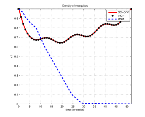
Figure 4.4: Density of mosquitoes

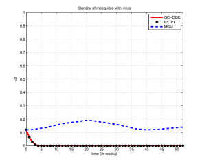
Figure 4.5: Infected mosquitoes

Figures 4.7 and 4.7 report to the population in the risk area. Our solution shows that the number of ill people decreases quickly. This could explain why the motivation level to fight the mosquito is lower when compared to the previous solution proposed in [20].

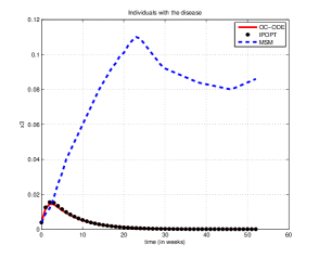
Figure 4.6: Infected individuals

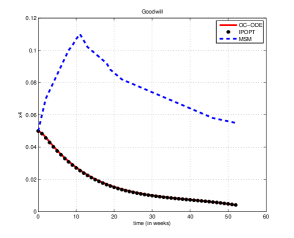
Figure 4.7: Level of popular motivation

Figure 4.8 shows the accumulated cost. It is clear that almost all year the cost is lower when compared with MSM [20]. This lower cost level is a consequence of infected mosquitos and infected individuals both falling down under our approach.

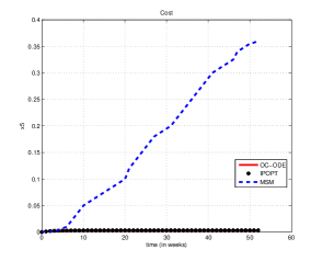
Figure 4.8: Cost

Figures 4.9 and 4.10 are related to the controls: educational campaigns and application of insecticides. It is possible to see that the new functions for the control variables are less expensive.

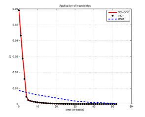
Figure 4.9: Application of insecticide

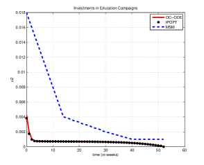
Figure 4.10: Educational campaigns

Despite the different philosophies of the OC-ODE (a specific control software) and Ipopt (a standard nonlinear optimization solver), the solution reached is similar. This fact enforces the robustness of the obtained results. It is important to mention that the problem under study is a difficult one. Other nonlinear packages were tested, and they could not reach a solution — some crashed at the middle or some bad scaling issues were observed.

Until some years ago, due to computational limitations, most of the models were run using codes made by the authors themselves as [20]. Nowadays, one can choose between several proper software packages ”out of the box”, that already take into account specific features of stiff problems, scaling problems, etc. With this work it is possible to realize that ”old” problems can again be taken into account and be better analyzed with new technology and approaches, with the goal of finding global optimal solutions, instead of local ones.

For this purpose, and at an initial research stage, it is important to understand if different kinds of discretization for an OC problem have influence on the problem resolution.

4.3 Using different discretization schemes

This section aims to study the costs of different discretization processes, in terms of time performance, number of variables and iterations used. For the purpose of this analysis two discretization schemes, Euler and second order Runge-Kutta’s scheme [9] (cf. Section 2.1), are considered to solve the problem described in the previous section.

This discretization process transforms the Dengue epidemics problem into a standard nonlinear optimization problem, with an objective function and a set of nonlinear constraints. This NLP problem was codified, for both discretization schemes, in the AMPL modeling language [55] and can be checked in [110].

Two nonlinear solvers with distinct features were selected to solve the NLP problem: the Knitro (IP method) and the Snopt (SQP method). The NEOS Server [98] platform was used as interface with both solvers. The Ipopt (IP method), used in the previous section, was the first choice for our research. However, at the time of this investigation, the NEOS platform was moved to another Center of Research and some software packages were unavailable for long periods of time. So, we had to choose another Interior Point robust software.

Table 4.1 reports the results for both solvers, for each discretization method using three different discretization steps ($h=0.5,0.25,0.125$), rising twelve numerical experiences. The columns # var. and # const. mean the number of variables and constraints, respectively. The next columns refer to the performance measures — number of iterations and total CPU time in seconds (time for solving the problem, for evaluate the objective and the constraints functions and for input/output). As the computational experiments were made in the NEOS server platform, the selected machine to run the program remains unknown as well as its technical specifications.

	Euler’s method	Runge-Kutta’s method
Knitro	h # var. # const. # iter. time (sec.) 0.5 727 519 113 2.090 0.25 1455 1039 68 2.210 0.125 2911 2079 85 7.240	h # var. # const. # iter. time (sec.) 0.5 728 520 64 1.980 0.25 1456 1040 82 5.550 0.125 2912 2080 70 9.740
Snopt	h # var. # const. # iter. time (sec.) 0.5 727 519 175 4.07 0.25 1455 1039 253 19.2 0.125 2911 2079 252 105.4	h # var. # const. # iter. time (sec.) 0.5 728 520 223 10.52 0.25 1456 1040 219 39.7 0.125 2912 2080 420 406.67

Table 4.1: Numerical results

The optimal cost reached was $\approx 3\times 10^{-3}$ for all tests. Comparing the general behavior of the solvers one can conclude that the IP based method (Knitro) presents much better performance than the SQP method (Snopt) in terms of the measures used. Regarding the Knitro results, one realizes that the Euler’s discretization scheme has better times for $h=0.25$ and $h=0.125$ and similar time for $h=0.5$, when compared to Runge-Kutta’s method. Another obvious finding, for both solvers, is that the CPU time increases as far as the problem dimension increases (number of variables and constraints). With respect to the number of iterations, Snopt presents more iterations as the problem dimension increases. However this conclusion cannot be taken for Knitro — in fact, there does not exist a relation between the problem dimension and the number of iterations. The best version tested was Knitro using Runge-Kutta with $h=0.5$ (best CPU time and fewer iterations), and the second one was Knitro with Euler’s method using $h=0.25$. An important evidence of this numerical experience is that it is not worth the reduction of the discretization step size because no significative advantages are obtained.

4.4 Conclusions

At this moment, as a result of major demographic changes, rapid urbanization on a massive scale, global travel and environmental change, the world faces enormous future challenges from emerging infectious diseases. Dengue illustrates well these challenges [141]. In this work we investigated an optimal control model for Dengue epidemics proposed in [20], that includes the mosquitoes dynamics, the effect of educational campaigns. The cost functional reflects a compromise between financial spending in insecticides and educational campaigns and the population health. For comparison reasons, the same choice of data/parameters in [20] was considered.

The results obtained from OC-ODE and Ipopt are similar, improving the ones previously reported in [20] (cf. Section 4.2). Indeed, the obtained control policy in this work presents an important progress with respect to the previous best policy: the percentage of infected mosquitoes vanishes just after four weeks, while mosquitoes are completely eradicated after 30 weeks (Figures 4.5 and 4.5); the number of infected individuals begin to decrease after four weeks while with the previous policy this only happens after 23 weeks (Figure 4.7). Despite the fact that our results are better, they are accomplished with a much smaller cost with insecticides and educational campaigns (Figure 4.8). The general improvement, which explains why the results are so successful, rely on an effective control policy of insecticides. The proposed strategy for insecticide application seems to explain the discrepancies between the results here obtained and the best policy of [20]. Our results show that applying insecticides in the first four weeks yields a substantial reduction in the cost of fighting Dengue, in terms of the functional proposed in [20]. The main conclusion is that health authorities should pay attention to the epidemic from the very beginning: effective control decisions in the first four weeks have a decisive role in the Dengue battle, and population and governments will both profit from it.

We successfully solved an OC problem by direct methods using nonlinear optimization software based on IP and SQP approaches. The problem was discretized through Euler and Runge-Kutta schemes. The implementation efforts of higher order discretization methods bring no advantages. The reduction of the discretization step and consequently the increase of the number of variables and constraints do not improve the performance with respect to the CPU time and to the number of iterations. We can point out the robustness of both solvers in spite of the dimension problem increase. The conclusions drawn in Section 4.3 were helpful for decision-making future processes of discretization all over the work.

As future work we intend to analyze how different parameters/weights associated to the variables in the objective function can influence the spread of the disease. This chapter was based on work available in the peer reviewed journal [112] and the peer reviewed conference proceedings [111].

Chapter 5 An ODE SEIR+ASEI model with an insecticide control

A model for the Dengue disease transmission is presented. It consists of eight mutually-exclusive compartments representing the human and vector dynamics. It also includes a control parameter, adulticide spray, as a measure to fight the disease. The model presents three possible equilibria: two Disease Free Equilibria (DFE) and an Endemic Equilibrium (EE). It has been proved that a DFE is locally asymptotically stable, whenever a certain epidemiological threshold, known as the basic reproduction number, is less than one. In this work we try to understand which is the best way to apply the control in order to effectively reduce the number of infected humans and mosquitoes. A case study, using outbreak data in 2009 in Cape Verde, is reported.

 

In Chapter 4 the Dengue epidemic was studied, mostly centered in people, specially in the goodwill of the individuals and spraying campaigns. However, the virus transmission scheme was overlooked: it was only considered two compartments for people and two compartments for adult mosquitoes. Here, the aim is to deepen the relationship between human and mosquitoes, creating a better framework to explain the development and transmission of the disease.

5.1 The SEIR+ASEI model

The mathematical model is based on [43, 44], that describes the chikungunya disease transmitted by Aedes albopictus.

The notation used in our mathematical model includes four epidemiological states for humans:

$S_{h}(t):$	susceptible
$E_{h}(t):$	exposed
$I_{h}(t):$	infected
$R_{h}(t):$	resistant

It is assumed that the total human population $(N_{h})$ is constant, so, $N_{h}=S_{h}+E_{h}+I_{h}+R_{h}$. There are also four other state variables related to the female mosquitoes (the male mosquitoes are not considered in this study because they do not bite humans and consequently they do not influence the dynamics of the disease):

$A_{m}(t):$	aquatic phase
$S_{m}(t):$	susceptible
$E_{m}(t):$	exposed
$I_{m}(t):$	infected

Similarly, it is assumed that the total adult mosquito population is constant, which means $N_{m}=S_{m}+E_{m}+I_{m}$. In this way, we put our model more complex and reliable to the reality of Dengue epidemics. For this study we introduced a control variable:

$c(t):$

level of insecticide campaigns

The control variable, $c(t)$, varies from 0 to 1. However, the model does not fit completely the reality. Epidemiologist and policy makers need to be aware of both strengths and weakness of the epidemiological modeling approach. An epidemiological model is always a simplification of reality. So, some assumptions were made to built this model:

• the total human population ($N_{h}$) is constant;

• there is no immigration of infected individuals into the human population;

• the population is homogeneous, which means that every individual of a compartment is homogenously mixed with the other individuals;

• the coefficient of transmission of the disease is fixed and does not vary seasonally;

• both human and mosquitoes are assumed to be born susceptible, i.e., there is no natural protection;

• for the mosquito there is no resistant phase, due to its short lifetime.

To completely describe the model it is necessary to use parameters, which are:

$N_{h}:$	total population
$B:$	average daily biting (per day)
$\beta_{mh}:$	transmission probability from $I_{m}$ (per bite)
$\beta_{hm}:$	transmission probability from $I_{h}$ (per bite)
$1/\mu_{h}:$	average lifespan of humans (in days)
$1/\eta_{h}:$	mean viremic period (in days)
$1/\mu_{m}:$	average lifespan of adult mosquitoes (in days)
$\varphi:$	number of eggs at each deposit per capita (per day)
$\mu_{A}:$	natural mortality of larvae (per day)
$\eta_{A}:$	maturation rate from larvae to adult (per day)
$1/\eta_{m}:$	extrinsic incubation period (in days)
$1/\nu_{h}:$	intrinsic incubation period (in days)
$m:$	female mosquitoes per human
$k:$	number of larvae per human
$K:$	maximal capacity of larvae

For notation simplicity, the independent variable $t$ will be omitted when writing the dependent variables, example given, will be written $S_{h}$ instead of $S_{h}(t)$. The Dengue epidemic can be modelled by the following nonlinear time-varying state equations:

Human Population

$$\left\{\begin{array}[]{l}\displaystyle\frac{dS_{h}}{dt}=\mu_{h}N_{h}-(B\beta_{mh}\frac{I_{m}}{N_{h}}+\mu_{h})S_{h}\\ \displaystyle\frac{dE_{h}}{dt}=B\beta_{mh}\frac{I_{m}}{N_{h}}S_{h}-(\nu_{h}+\mu_{h})E_{h}\\ \displaystyle\frac{dI_{h}}{dt}=\nu_{h}E_{h}-(\eta_{h}+\mu_{h})I_{h}\\ \displaystyle\frac{dR_{h}}{dt}=\eta_{h}I_{h}-\mu_{h}R_{h}\end{array}\right.$$

(5.1)

and vector population

$$\left\{\begin{array}[]{l}\displaystyle\frac{dA_{m}}{dt}=\varphi(1-\frac{A_{m}}{kN_{h}})(S_{m}+E_{m}+I_{m})-(\eta_{A}+\mu_{A})A_{m}\\ \displaystyle\frac{dS_{m}}{dt}=\eta_{A}A_{m}-(B\beta_{hm}\frac{I_{h}}{N_{h}}+\mu_{m})S_{m}-cS_{m}\\ \displaystyle\frac{dE_{m}}{dt}=B\beta_{hm}\frac{I_{h}}{N_{h}}S_{m}-(\mu_{m}+\eta_{m})E_{m}-cE_{m}\\ \displaystyle\frac{dI_{m}}{dt}=\eta_{m}E_{m}-\mu_{m}I_{m}-cI_{m}\\ \end{array}\right.$$

(5.2)

with the initial conditions

$$S_{h}(0)=S_{h0},$$

(5.3)

Figure 5.1 shows the relation between human and mosquito and the corresponding parameters.

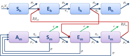
Figure 5.1: Epidemiological model SEIR+ASEI

Notice that the equation related to the aquatic phase does not have the control variable $c$, because the adulticide does not produce effects in this stage of mosquito life. To fight the larval phase it would be necessary to use larvicide. This treatment should be long-lasting and have World Health Organization clearance for use in drinking water. As we want to study only a short period of time, this type of treatment has not been considered here.

With the condition $S_{h}+E_{h}+I_{h}+R_{h}=N_{h}$, one can, in the example given, use $R_{h}=N_{h}-S_{h}-E_{h}-I_{h}$ and consider an equivalent system for human population without considering the $R_{h}$ differential equation.

For the previous set of differential equations is now analyzed the equilibrium points of the system and is determined the threshold phenomena.

5.1.1 Basic reproduction number, equilibrium points and stability

Let the set

$\Omega=\{(S_{h},E_{h},I_{h},A_{m},S_{m},E_{m},I_{m})\in\mathbb{R}^{7}_{+}:$

$S_{h}+E_{h}+I_{h}\leq N_{h},A_{m}\leq kN_{h},S_{m}+E_{m}+I_{m}\leq mN_{h}\}$

be the region of biological interest.

Proposition 4.

$\Omega$ is positively invariant under the flow induced by the differential system (5.1)-(5.2).

Proof.

System (5.1)–(5.2) can be rewritten in the following way:

$$\frac{dX}{dt}=M(X)X+F$$ (5.4)

where $X=\left(S_{h},E_{h},I_{h},A_{m},S_{m},E_{m},I_{m}\right)$, $F=\left(\mu_{h}N_{h},0,0,0,0,0,0\right)^{T}$ and

$M(X)=\left(\begin{array}[]{ccccccc}-B\beta_{mh}\frac{I_{m}}{N_{h}}-\mu_{h}&0&0&0&0&0&0\\ B\beta_{mh}\frac{Im}{N_{h}}&-\nu_{h}-\mu_{h}&0&0&0&0&0\\ 0&\nu_{h}&-\eta_{h}-\mu_{h}&0&0&0&0\\ 0&0&0&\Upsilon&\mu_{b}&\mu_{b}&\mu_{b}\\ 0&0&0&\eta_{A}&\Theta&0&0\\ 0&0&0&0&B\beta_{hm}\frac{I_{h}}{N_{h}}&\Psi&0\\ 0&0&0&0&0&\eta_{m}&-\mu_{m}-c\\ \end{array}\right)$,

with $\Upsilon=-\mu_{b}\frac{S_{m}+E_{m}+I_{m}}{K}-\mu_{m}-\eta_{m}$, $\Theta=-B\beta_{hm}\frac{I_{h}}{N_{h}}-\mu_{m}-c$ and $\Psi=-\mu_{m}-\eta_{m}-c$.

As $M(X)$ has all off-diagonal entries nonnegative, $M(X)$ is a Metzler matrix.

Using the fact that $F\geq 0$, the system (5.4) is positively invariant in $\mathbb{R}^{7}_{+}$ [1], which means that any trajectory of the system starting from an initial state in the positive orthant $\mathbb{R}^{7}_{+}$ remains forever in $\mathbb{R}^{7}_{+}$. ∎

Theorem 5.1.1.

Let $\Omega$ be defined as above. Consider also

$\mathcal{M}=-\left(c(\eta_{A}+\mu_{A})+\mu_{A}\mu_{m}+\eta_{A}(-\varphi+\mu_{m})\right)$.

The system (5.1)–(5.2) admits at most two Disease Free Equilibrium points:

• if $\mathcal{M}\leq 0$, there is a Disease Free Equilibrium (DFE),

  $$E_{1}^{*}=\left(N_{h},0,0,0,0,0,0\right),$$

  called Trivial Equilibrium;

• if $\mathcal{M}>0$, there is a Biologically Realistic Disease Free Equilibrium (BRDFE),

  $$E_{2}^{*}=\left(N_{h},0,0,\frac{kN_{h}\mathcal{M}}{\eta_{A}\varphi},\frac{kN_{h}\mathcal{M}}{\varphi\mu_{m}},0,0\right).$$

Proof.

The equilibrium points are reached when the following equations hold:

$$\left\{\begin{array}[]{l}\frac{dS_{h}}{dt}=0\\ \frac{dE_{h}}{dt}=0\\ \frac{dI_{h}}{dt}=0\\ \frac{dR_{h}}{dt}=0\\ \frac{dA_{m}}{dt}=0\\ \frac{dS_{m}}{dt}=0\\ \frac{dE_{m}}{dt}=0\\ \frac{dI_{m}}{dt}=0\\ \end{array}\right.$$

(5.5)

Using the Mathematica software to solve the system (5.5), we obtained four solutions.

The first one is known as the Trivial Equilibrium, since the mosquitoes do not exist, so there is no disease:

$E_{1}^{*}=\left(N_{h},0,0,0,0,0,0\right)$

In the second one, mosquitoes and humans interact, but there is only one outbreak of the disease, i.e., over time the disease goes away without killing all the mosquitoes. We have called this equilibrium point a Biologically Realistic Disease Free Equilibrium (BRDFE), since it is a more reasonable situation to find in nature than the previous one:

$E_{2}^{*}=$	$\left(N_{h},0,0,\displaystyle\frac{kNh(-\left(c(\eta_{A}+\mu_{A})+\mu_{A}\mu_{m}+\eta_{A}(-\mu_{b}+\mu_{m})\right))}{\eta_{A}\mu_{b}},\right.$
	$\displaystyle\left.\frac{kNh(-\left(c(\eta_{A}+\mu_{A})+\mu_{A}\mu_{m}+\eta_{A}(-\mu_{b}+\mu_{m})\right))}{\mu_{b}\mu_{m}},0,0\right)$,

which is equivalent to $E_{2}^{*}=\left(N_{h},0,0,\frac{kNh\mathcal{M}}{\eta_{A}\mu_{b}},\frac{kNh\mathcal{M}}{\mu_{b}\mu_{m}},0,0\right)$. This is biologically interesting only if $\mathcal{M}$ is greater than 0.

The third solution corresponds to a situation where humans and mosquitoes live together but the disease persists in both populations, which means that it is not a DFE. This equilibrium will be explained after (see Theorem 5.1.3). Thus the disease is not anymore an epidemic episode, but transforms into a endemic one. With some algebraic manipulations we obtained the following point:

$E_{3}^{*}=\left(S_{h}^{*},E_{h}^{*},I_{h}^{*},A_{m}^{*},S_{m}^{*},E_{m}^{*},I_{m}^{*}\right)$ where,

$S_{h}^{*}=N_{h}-\displaystyle\frac{(\mu_{h}+\nu_{h})(\mu_{h}+\eta_{h})}{\mu_{h}\nu_{h}}I_{h}^{*}$,

$E_{h}^{*}=\displaystyle\frac{\mu_{h}+\eta_{h}}{\nu_{h}}I^{*}_{h}$,

$I_{h}^{*}=N_{h}\mu_{h}(-B^{2}k\beta_{hm}\beta_{mh}\nu_{h}\eta_{m}\mathcal{M}+\mu_{b}\mu_{m}^{2}(\eta_{m}+\mu_{m})(\mu_{h}+\ \nu_{h})(\mu_{h}+\eta_{h})+c^{2}\mu_{b}(\eta_{h}+\mu_{h})(\mu_{h}+\nu_{h})(c+\eta_{m}+3\mu_{m})+c\mu_{b}\mu_{m}(\mu_{h}+\nu_{h})(\mu_{h}(3\mu_{m}+2)+\eta_{h}(2\eta_{m}+3\mu_{m})))/(B\beta_{hm}(\eta_{h}+\mu_{h})(-\mu_{b}\mu_{h}\ (c+\mu_{m})(c+\eta_{m}+\mu_{m})-Bk\beta_{mh}\eta_{m}\mathcal{M})(\mu_{h}+\nu_{h}))$;

$A_{m}^{*}=\displaystyle\frac{\mathcal{M}}{\eta_{A}\mu_{b}}kN_{h}$,

$S_{m}^{*}=\displaystyle\frac{kNh^{2}\mathcal{M}}{\mu_{b}(cN_{h}+BI_{h}^{*}\beta_{hm}+N_{h}\mu_{m})}$,

$E_{m}^{*}=\displaystyle\frac{\mu_{m}+c}{\eta_{m}}I_{m}^{*}$,

$I_{m}^{*}=\displaystyle\frac{BI_{h}^{*}kN_{h}\beta_{hm}\eta_{m}\mathcal{M}}{\mu_{b}(c+\mu_{m})(c+\eta_{m}+\mu_{m})(cN_{h}+BI_{h}^{*}\beta_{hm}+N_{h}\mu_{m})}$

As before, this equilibrium is only biologically interesting if $\mathcal{M}>0$.

With the Mathematica software we obtained a fourth solution. But some of the components are negative, which means that they do not belong to the $\Omega$ set. ∎

Remark 6.

The condition $\mathcal{M}>0$ is equivalent, by algebraic manipulation, to the condition

$$\frac{(\eta_{A}+\mu_{A})(\mu_{m}+c)}{\varphi\eta_{A}}<1,$$

which corresponds to the basic offspring number for mosquitoes. Thus, if $\mathcal{M}<0$, then the mosquito population will collapse and the only equilibrium for the whole system is the trivial equilibrium. If $\mathcal{M}\geq 0$, then the mosquito population is sustainable.

The amount of mosquitoes is also related to an epidemic threshold: the basic reproduction number of the disease, $\mathcal{R}_{0}$. Following [42], we prove:

Theorem 5.1.2.

If $\mathcal{M}>0$, then the square of the basic reproduction number associated to (5.1)-(5.2) is

$$\mathcal{R}_{0}^{2}=\displaystyle\frac{B^{2}S_{h0}S_{m0}\beta_{hm}\beta_{mh}\eta_{m}\nu_{h}}{N_{h}^{2}(\eta_{h}+\mu_{h})(c+\mu_{m})(c+\eta_{m}+\mu_{m})(\mu_{h}+\nu_{h})}.$$

The equilibrium point BRDFE is locally asymptotically stable if $\mathcal{R}_{0}<1$ and unstable if $\mathcal{R}_{0}>1$.

Proof.

To derive the basic reproduction number, we use the next generator approach. The basic reproduction number is calculated in a Disease Free Equilibrium. In this case we consider the most realistic one, BRDFE.

Following [3, 42], let consider the vector $x^{T}=\left(E_{h},I_{h},E_{m},I_{m}\right)$ which corresponds to the components related to the progression of the disease.

The subsystem used is:

$$\left\{\begin{array}[]{l}\frac{dE_{h}}{dt}=B\beta_{mh}\frac{Im}{N_{h}}S_{h}-(\nu_{h}+\mu_{h})E_{h}\\ \frac{dI_{h}}{dt}=\nu_{h}E_{h}-(\eta_{h}+\mu_{h})I_{h}\\ \frac{dE_{m}}{dt}=B\beta_{hm}\frac{I_{h}}{N_{h}}S_{m}-(\mu_{m}+\eta_{m})E_{m}-cE_{m}\\ \frac{dI_{m}}{dt}=\eta_{m}E_{m}-\mu_{m}I_{m}-cI_{m}\end{array}\right.$$

(5.6)

This subsystem can be partitioned, $\displaystyle\frac{dx}{dt}=\mathcal{F}(x)-\mathcal{V}(x)$, where $x^{T}=\left(E_{h},I_{h},E_{m},I_{m}\right)$, $\mathcal{F}(x)$ represents the components related to new cases of disease (in this situation in the exposed compartments) and $\mathcal{V}(x)$ represents the other components. Thus the subsystem (5.6) can be rewritten as

$\mathcal{F}(x)=\left(\begin{array}[]{c}B\beta_{mh}\frac{I_{m}}{N_{h}}S_{h}\\ 0\\ B\beta_{hm}\frac{I_{h}}{N_{h}}S_{m}\\ 0\\ \end{array}\right)$ and $\mathcal{V}(x)=\left(\begin{array}[]{c}(\nu_{h}+\mu_{h})E_{h}\\ -\nu_{h}E_{h}+(\eta_{h}+\mu_{h})I_{h}\\ (\mu_{m}+\eta_{m}+c)E_{m}\\ -\eta_{m}E_{m}+(\mu_{m}+c)I_{m}\\ \end{array}\right).$

Let us consider the Jacobian matrices associated with $\mathcal{F}$ and $\mathcal{V}$:

$J_{\mathcal{F}(x)}=\left(\begin{array}[]{cccc}0&0&0&B\beta_{mh}\frac{S_{h}}{N_{h}}\\ 0&0&0&0\\ 0&B\beta_{hm}\frac{S_{m}}{N_{h}}&0&0\\ 0&0&0&0\\ \end{array}\right)$

and

$J_{\mathcal{V}(x)}=\left(\begin{array}[]{cccc}\nu_{h}+\mu_{h}&0&0&0\\ -\nu_{h}&\eta_{h}+\mu_{h}&0&0\\ 0&0&\mu_{m}+\eta_{m}+c&0\\ 0&0&-\eta_{m}&\mu_{m}+c\\ \end{array}\right).$

According to [42] the basic reproduction number is $\mathcal{R}_{0}=\rho(J_{\mathcal{F}(x_{0})}J_{\mathcal{V}^{-1}(x_{0})})$, where $x_{0}$ is a Disease Free Equilibrium (BRDFE) and $\rho(A)$ defines the spectral radius of a matrix $A$. Using Mathematica

$\mathcal{R}_{0}^{2}=\displaystyle\frac{B^{2}k\beta_{hm}\beta_{mh}\eta_{m}\nu_{h}\mathcal{M}}{\mu_{b}(\eta_{h}+\ \mu_{h})(c+\mu_{m})^{2}(c+\eta_{m}+\mu_{m})(\mu_{h}+\nu_{h})}$

and we obtain the value for the threshold parameter, with $\mathcal{M}>0$. ∎

Remark 7.

In the model we have two different populations (human and vectors), so the expected basic reproduction number reflects the infection human-vector and also vector-human, that is, $\mathcal{R}_{0}^{2}=R_{hm}\times R_{mh}$. The term $B\beta_{hm}\frac{S_{m0}}{N_{h}}$ represents the product between the transmission probability of the disease from humans to vectors and the number of susceptible mosquitoes per human; $\frac{1}{\eta_{h}+\mu_{h}}$ is related to the human’s viremic period; and $\frac{\eta_{m}}{c+\eta_{m}+\mu_{m}}$ represents the proportion of mosquitoes that survive to the incubation period. Analogously, the term $B\beta_{mh}\frac{S_{h0}}{Nh}$ is related to the transmission probability of the disease between mosquitos and human, in a susceptible population; $\frac{1}{(c+\mu_{m})}$ represents the lifespan of an adult mosquito; and $\frac{\nu_{h}}{(\mu_{h}+\nu_{h})}$ is the proportion of humans that survive the incubation period.

When $\mathcal{R}_{0}<1$, each infected individual produces, on average, less than one new infected individual, and therefore it is predictable that the infection will be cleared from the population. If $\mathcal{R}_{0}>1$, the disease is able to invade the susceptible population [42, 83].

Theorem 5.1.3.

If $\mathcal{M}>0$ and $\mathcal{R}_{0}>1$, then the system (5.1)-(5.2) also admits an endemic equilibrium (EE): $E_{3}^{*}=\left(S_{h}^{*},E_{h}^{*},I_{h}^{*},A_{m}^{*},S_{m}^{*},E_{m}^{*},I_{m}^{*}\right)$, where,

$$\begin{split}S_{h}^{*}&=N_{h}-\displaystyle\frac{(\mu_{h}+\nu_{h})(\mu_{h}+\eta_{h})}{\mu_{h}\nu_{h}}I_{h}^{*},\\ E_{h}^{*}&=\displaystyle\frac{\mu_{h}+\eta_{h}}{\nu_{h}}I^{*}_{h},\\ I_{h}^{*}&=\frac{\xi}{\chi},\\ \xi&=N_{h}\mu_{h}\Bigl{[}-B^{2}k\beta_{hm}\beta_{mh}\nu_{h}\eta_{m}\mathcal{M}+\varphi\mu_{m}^{2}(\eta_{m}+\mu_{m})(\mu_{h}+\nu_{h})(\mu_{h}+\eta_{h})\\ &\quad+c^{2}\varphi(\eta_{h}+\mu_{h})(\mu_{h}+\nu_{h})(c+\eta_{m}+3\mu_{m})\\ &\quad+c\varphi\mu_{m}(\mu_{h}+\nu_{h})(\mu_{h}(3\mu_{m}+2)+\eta_{h}(2\eta_{m}+3\mu_{m}))\Bigr{]},\\ \chi&=B\beta_{hm}(\eta_{h}+\mu_{h})\Bigl{[}-\varphi\mu_{h}(c+\mu_{m})(c+\eta_{m}+\mu_{m})-Bk\beta_{mh}\eta_{m}\mathcal{M}\Bigr{]}(\mu_{h}+\nu_{h}),\\ A_{m}^{*}&=\displaystyle\frac{\mathcal{M}}{\eta_{A}\varphi}kN_{h},\\ S_{m}^{*}&=\displaystyle\frac{kNh^{2}\mathcal{M}}{\varphi(cN_{h}+BI_{h}^{*}\beta_{hm}+N_{h}\mu_{m})},\\ E_{m}^{*}&=\displaystyle\frac{\mu_{m}+c}{\eta_{m}}I_{m}^{*},\\ I_{m}^{*}&=\displaystyle\frac{BI_{h}^{*}kN_{h}\beta_{hm}\eta_{m}\mathcal{M}}{\varphi(c+\mu_{m})(c+\eta_{m}+\mu_{m})(cN_{h}+BI_{h}^{*}\beta_{hm}+N_{h}\mu_{m})}.\end{split}$$

Proof.

See Proof of Theorem 5.1.1. ∎

From a biological point of view, it is desirable that humans and mosquitoes coexist without the disease reaching a level of endemicity. Good estimates of Dengue transmission intensity are therefore necessary to compare and interpret Dengue interventions conducted in different places and times and to evaluate options for Dengue control. The basic reproduction number has played a central role in the epidemiological theory for Dengue and other infectious diseases because it provides an index of transmission intensity and establishes a threshold criteria. We claim that proper use of control $c$, can result in the basic reproduction number remaining below unity and, therefore, making BRDFE stable. In order to make effective use of achievable insecticide control, and simultaneously to explain more easily to the competent authorities its effectiveness, we assume that $c$ is constant. The goal is to find $c$ such that $\mathcal{R}_{0}^{2}<1$. For this purpose we have studied the reality of Cape Verde.

5.1.2 Dengue in Cape Verde

An unprecedented outbreak was detected in the Cape Verde archipelago in September 2009. This is the first report of Dengue virus activity in that country. As the population had never had contact with the virus, the herd immunity was very low. Dengue type 3 spread throughout the islands of the archipelago, reaching four of the nine islands. The worst outbreak occurred on the Santiago island, where most people live. The number of cases increased sharply since the beginning of November, reaching 1000 cases per day. The Cape Verde Ministry of Health reported more than 20000 cases of Dengue Fever within the archipelago between October and December 2009, which is about 5% of the total population of the country. From 173 cases of Dengue hemorrhagic fever reported, six people died [31, 40].

It represented a challenge to the performance of the National Health Care System. Government officials launched a plan to eradicate the mosquito including a national holiday during which citizens were being asked to clear out standing water and other potential breeding areas used by the mosquitoes. The intense and spontaneous movement of solidarity from the civil society was another noteworthy dimension, not only cleaning but also voluntary donating blood to strengthen the stock of the Central Hospital Dr. Agostinho Neto, in Praia.

We used the data for human population related to Cape Verde [54]. Due to low surveillance and the fact of being the first ever of Dengue outbreak in the country, it was not possible to collect detailed data from the mosquito. However, the authorities speak explicitly about mosquitoes coming from Brazil [2]. Also the information that comes from the Ministry of Health in the capital of Cape Verde, Praia, confirms that the insects responsible for Dengue came most probably from Brazil, transported by means of air transport that perform frequent connections between Cape Verde and Brazil, as reported by the Radio of Cape Verde. With respect to Aedes aegypti, we have thus considered data from Brazil [132, 143].

The simulations were carried out using the following values: $N_{h}=480000$, $B=1$, $\beta_{mh}=0.375$, $\beta_{hm}=0.375$, $\mu_{h}=1/(71\times 365)$, $\eta_{h}=1/3$, $\mu_{m}=1/11$, $\varphi=6$, $\mu_{A}=1/4$, $\eta_{A}=0.08$, $\eta_{m}=1/11$, $\nu_{h}=1/4$, , $m=6$, $k=3$. The initial conditions for the problem were: $S_{h0}=N_{h}-E_{h}-I_{h}$, $E_{h0}=216$, $I_{h0}=434$, $R_{h0}=0$, $A_{m0}=kN_{h}$, $S_{m0}=mN_{h}$ and $I_{m0}=0$.

Considering nonexistence of control, i.e. $c=0$, the basic reproduction number for this outbreak in Cape Verde is approximately $\mathcal{R}_{0}=2.396$, which is in agreement to other studies of Dengue in other countries [100]. The control $c$ affects the basic reproduction number, and our aim is to find a control that puts $\mathcal{R}_{0}$ less than one.

Proposition 5.

Let us consider the parameters listed above and consider $c$ as a constant. Then $\mathcal{R}_{0}<1$ if and only if $c>0.156961$.

This value was obtained by Mathematica, calculating the inequality with the parameters values above. The computational investigations were carried out using $c=0.157$, which means that the insecticide is continuously applied during a twelve week period.

The software used was Scilab [21]. It is an open source, cross-platform numerical computational package and a high-level, numerically oriented programming language. For our problem we used the routine ode to solve the set of differential equations. By default, ode uses the lsoda solver of package ODEPACK. It automatically selects between the nonstiff predictor-corrector Adams method and the stiff Backward Differentiation Formula (BDF) method. It uses the nonstiff method initially and dynamically monitors data in order to decide which method to use. The graphics were also obtained using this software, with the command plot (see code in [110]).

Figures 5.2 and 5.3 show the curves related to human population, with and without control, respectively. The number of infected people, even with small control, is much less than without any insecticide campaign.

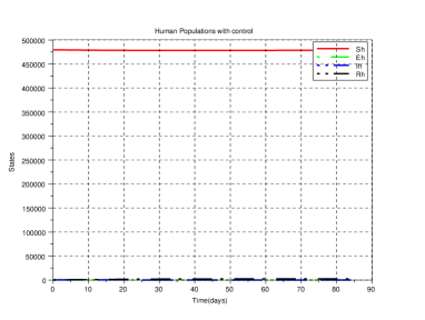
Figure 5.2: Human compartments using control

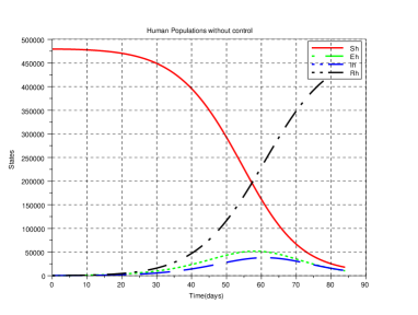
Figure 5.3: Human compartments without control

Figures 5.4 and 5.5 show the difference of the mosquito population with control and without control. When the control is applied, the number of infected mosquitoes is close to zero. Note that the intention is not to completely eradicate the mosquitoes but instead the number of infected mosquitoes.

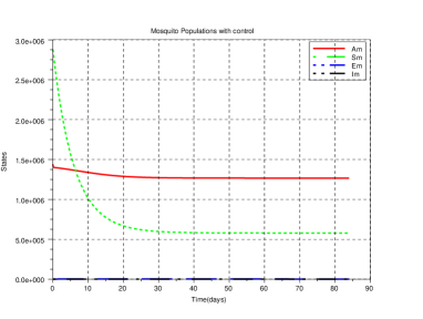
Figure 5.4: Mosquito compartments using control

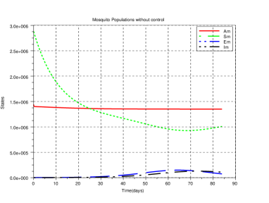
Figure 5.5: Mosquito compartments without control

It has been algebraically proved that if a constant minimum level of a control is applied ($c=0.157$), it is possible to maintain the basic reproduction number below unity, guaranteeing the BRDFE. This value is corroborated in another numerical study [113].

The values of infected humans obtained by the model are higher when compared to what really happened in Cape Verde. Despite the measures taken by the government and Health authorities were not accounted, they have had a considerable impact in the progress of the disease.

Until here, it was considered a constant control. Using a theoretical approach [112], we intend to find the best function $c(t)$, using OC theory. Instead of finding a constant control it will be possible to study other types of control, such as piecewise constant or even continuous but not constant. Additionally we could consider another strategy, a more practical one: due to logistics and health reasons, it may be more convenient to apply insecticide periodically and at some specific hours at night.

5.2 Insecticide control in a Dengue epidemics model

In this section we investigate the best way to apply the control in order to effectively reduce the number of infected humans and mosquitoes, using pulse control.

In literature it has been proven that a DFE is locally asymptotically stable, whenever a certain epidemiological threshold, known as the basic reproduction number, is less than one. In the previous section, it was proven that if a constant minimum level of insecticide is applied ($c=0.157$), it is possible to maintain the basic reproduction number below unity, guaranteeing the DFE. In this section, other kinds of piecewise controls that maintain the basic reproduction number less than one and could give a better solution to implement by health authorities are investigated.

To solve the system (5.1)–(5.2), in a first step, several strategies of control application were used: three different frequencies (weekly, bi-weekly and monthly) for control application, a constant control ($c=0.157$) and no control ($c=0$). The first three different frequencies mean that during one day (per week, bi-week and month), the whole ($100\%$) capacity of insecticide ($c=1$) is used during all day. Besides, also was used a constant control strategy ($c=0.157$) that consists in the application of $15.7\%$ capacity of insecticide 24 hours per day all the time (84 days). In this work, the amount of insecticide is an adimensional value and must be considered in relative terms.

The numerical tests were carried out using Scilab [120], with the same ODE system and parameters of the previous section (code available in [110]).

Figures 5.6 and 5.7 show the results of these strategies regarding infected mosquitoes and individuals. Without control, the number of infected mosquitoes and individuals increase expressively. It is also possible to see that the weekly pulse control had the closest results to the continuous control.

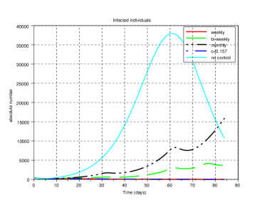
Figure 5.6: Comparison of infected humans using no control, continuous control and periodically control (weekly, biweekly and monthly)

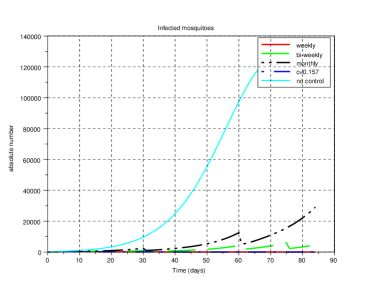
Figure 5.7: Comparison of infected mosquitoes using no control, continuous control and periodically control (weekly, biweekly and monthly)

Therefore, realizing the influence of the insecticide control, further tests were carried out to find the optimum periodicity of administration which, from gathered results, must rest between six and seven days. The second phase of numerical tests, Figures 5.8 and 5.9, considered four situations: 6 days, 7 days, 10 days and continuously $c=0.157$. To guarantee the DFE, the curves must remain below the one corresponding to $c=0.157$.

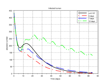
Figure 5.8: Infected human and different piecewise controls

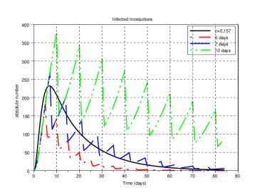
Figure 5.9: Infected mosquitoes and different piecewise controls

The amount of insecticide, and when to apply it, are important factors for outbreak control. Table 5.1 reports the total amount of insecticide used in each version during the 84 days.

	6 days	7 days	10 days	15 days	30 days	$c=0.157$
insecticide amount	14	12	9	6	3	13.188

Table 5.1: Insecticide cost

The numerical tests conclude that the best strategy for the infected reduction is every 6/7 days application. The value spent in insecticide is similar to the continuous strategy, but is much easier to implement in terms of logistics of a massive application. This result is consistent with what WHO recommends, which is an application of insecticide every 3/4 days; this lower frequency is probably due to the non-application of insecticide during all day.

In this work, several piecewise strategies were studied to find the best way of applying insecticide, but always having in mind a periodic application of the product. But if the best strategy is not a periodic one? In the next section the optimal control solution for this problem will be studied.

5.3 Optimal control

The aim of this section is the study of optimal strategies for applying insecticide, taking into account different perspectives: thinking only on the insecticide cost, focusing on the cost of infected humans or even combining both perspectives.

To take this approach, and after several numerical experiences, we considered that it was better to normalize the ODE system (5.1)–(5.2). The reason for this transformation is due to the bad scaling of the variables: some vary from 0 to 480000, and others from 0 to 1, which can influence the software performance.

Consider the following transformations:

$\displaystyle s_{h}=\frac{S_{h}}{N_{h}}$	$\displaystyle e_{h}=\frac{E_{h}}{N_{h}}$	$\displaystyle i_{h}=\frac{I_{h}}{N_{h}}$	$\displaystyle r_{h}=\frac{R_{h}}{N_{h}}$
$\displaystyle a_{m}=\frac{A_{h}}{kN_{h}}$	$\displaystyle s_{m}=\frac{S_{m}}{mN_{h}}$	$\displaystyle e_{m}=\frac{E_{m}}{mN_{h}}$	$\displaystyle i_{m}=\frac{I_{m}}{mN_{h}}$

The ODE system (5.1)–(5.2) is transformed into:

$$\left\{\begin{array}[]{l}\displaystyle\frac{ds_{h}}{dt}=\mu_{h}-(B\beta_{mh}mi_{m}+\mu_{h})s_{h}\\ \displaystyle\frac{de_{h}}{dt}=B\beta_{mh}mi_{m}s_{h}-(\nu_{h}+\mu_{h})e_{h}\\ \displaystyle\frac{di_{h}}{dt}=\nu_{h}e_{h}-(\eta_{h}+\mu_{h})i_{h}\\ \displaystyle\frac{dr_{h}}{dt}=\eta_{h}i_{h}-\mu_{h}r_{h}\\ \displaystyle\frac{da_{m}}{dt}=\varphi\frac{m}{k}(1-a_{m})(s_{m}+e_{m}+i_{m})-(\eta_{A}+\mu_{A})a_{m}\\ \displaystyle\frac{ds_{m}}{dt}=\eta_{A}\frac{k}{m}a_{m}-(B\beta_{hm}i_{h}+\mu_{m})s_{m}-cs_{m}\\ \displaystyle\frac{de_{m}}{dt}=B\beta_{hm}i_{h}s_{m}-(\mu_{m}+\eta_{m})e_{m}-ce_{m}\\ \displaystyle\frac{di_{m}}{dt}=\eta_{m}e_{m}-\mu_{m}i_{m}-ci_{m}\\ \end{array}\right.$$

(5.7)

with the initial conditions

$$s_{h}(0)=0.99865,$$

(5.8)

Let $x=(s_{h},e_{h},i_{h},r_{h},a_{m},s_{m},e_{m},i_{m})$ the vector representing the state variables.

Let us consider the objective functional $J$ considering the costs of infected humans and costs with insecticide:

$$\text{minimize }J=\int_{0}^{t_{f}}\left[\gamma_{D}i_{h}(t)^{2}+\gamma_{S}c(t)^{2}\right]dt,$$ (5.9)

where $\gamma_{D}$ and $\gamma_{S}$ are positive constants representing the costs weights of infected individuals and spraying campaigns, respectively.

5.3.1 Pontryagin’s Maximum Principle

Using OC theory, let $\lambda_{i}(t)$, with $i=1,\ldots,8$, be the co-state variables. The Hamiltonian for the present OC problem is given by

$$H$$ =

(5.10)

By the Pontryagin Maximum Principle [106], the optimal control $c^{*}$ should be the one that minimizes, at each instant $t$, the Hamiltonian given by (5.10), that is, $H\left(x^{*}(t),\lambda^{*}(t),c^{*}(t)\right)=\min_{c\in[0,1]}H\left(x^{*}(t),\lambda^{*}(t),c\right)$. In this way, the optimal control is given by

$$c^{*}=\min\left\{1,\max\left\{0,\frac{\lambda_{6}s_{m}+\lambda_{7}e_{m}+\lambda_{8}i_{m}}{2\gamma_{S}}\right\}\right\}.$$

It is also necessary to consider the adjoint system $\lambda^{{}^{\prime}}_{i}(t)=-\displaystyle\frac{\partial H}{\partial x_{i}}$, i.e.,

$$\left\{\begin{array}[]{l}\lambda_{1}^{{}^{\prime}}=\lambda_{1}\left(B\beta_{mh}mi_{m}+\mu_{h}\right)-\lambda_{2}B\beta_{mh}mi_{m}\\ \lambda_{2}^{{}^{\prime}}=\lambda_{2}\left(\nu_{h}+\mu_{h}\right)-\lambda_{3}\nu_{h}\\ \lambda_{3}^{{}^{\prime}}=-2\gamma_{D}i_{h}+\lambda_{3}\left(\eta_{h}+\mu_{h}\right)-\lambda_{4}\eta_{h}+(\lambda_{6}-\lambda_{7})B\beta_{hm}s_{m}\\ \displaystyle\lambda_{4}^{{}^{\prime}}(t)=\lambda_{4}\mu_{h}\\ \lambda_{5}^{{}^{\prime}}=\lambda_{5}\left[\varphi\frac{m}{k}\left(s_{m}+e_{m}+i_{m}\right)+\eta_{A}+\mu_{A}\right]-\lambda_{6}\eta_{A}\frac{k}{m}\\ \lambda_{6}^{{}^{\prime}}=-\lambda_{5}\varphi\frac{m}{k}\left(1-a_{m}\right)+\lambda_{6}\left(B\beta_{hm}i_{h}+\mu_{m}+c\right)-\lambda_{7}B\beta_{hm}i_{h}\\ \lambda_{7}^{{}^{\prime}}=-\lambda_{5}\varphi\frac{m}{k}\left(1-a_{m}\right)+\lambda_{7}(\mu_{m}+\eta_{m}+c)-\lambda_{8}\eta_{m}\\ \lambda_{8}^{{}^{\prime}}=\left(\lambda_{1}-\lambda_{2}\right)B\beta_{mh}ms_{h}-\lambda_{5}\varphi\frac{m}{k}\left(1-a_{m}\right)+\lambda_{8}\left(\mu_{m}+c\right)\\ \end{array}\right.$$

(5.11)

As the OC problem just has initial conditions it is necessary to find the transversality conditions, that correspond to a terminal condition in the co-state equation,

$$\lambda_{i}(t_{f})=0$$

(5.12)

Replacing the optimal control $c^{*}$ in the state system (5.7) and in the adjoint system (5.11) is possible to solve the differential system taking into account the initial and transversality conditions.

5.3.2 Numerical simulations

In order to solve this OC problem three approaches were tested. The first one is a direct method, DOTcvp toolbox [67] for Matlab. It uses the differential system (5.7), the initial conditions (5.8) and it is necessary to transform the problem into a Mayer form (see Section 2.3). To solve the discretized OC problem, the Ipopt software is chosen as an option inside the DOTcvp. The functional is divided into time intervals, in this case ten intervals, with an initial value problem tolerance of $10^{-7}$ and a NLP tolerance of $10^{-5}$. The optimal control function given by this toolbox is piecewise constant.

Another direct method is OC-ODE [57]. It uses the differential system (5.7), the initial conditions (5.8) and it includes procedures for numerical adjoint estimation and sensitivity analysis and the feasibility tolerance considered was $10^{-10}$.

The last method used, an indirect one, it is coded in Matlab environment. It involves the backward-forward method (see Section 2.2) and the resolution of the ODE systems are made by the ode45 routine. The state differential system (5.7) is solved forward with initial conditions (5.8), while the adjoint system (5.11) is solved backwards using the terminal conditions (5.12). The absolute and relative tolerances were fixed in $10^{-4}$. The three codes are available at [110].

All the parameters are assumed equal to the previous section. For this first simulation, the values for the weights of the costs are $\gamma_{D}=0.5$ and $\gamma_{S}=0.5$.

Figure 5.10 shows that, despite having distinct philosophies of resolution, the curves obtained by the three solvers are similar, which reinforces the confidence in the result.

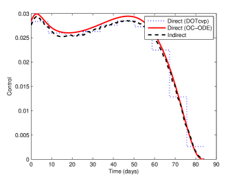
Figure 5.10: Optimal control obtained by the three methods

Figure 5.11 presents the number of infected humans over the 84 days. The tendency curve is similar, but the indirect method presents a higher number of infected people.

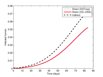
Figure 5.11: Infected human obtained by the three methods

The optimal functional is 0.0470, 0.0498 and 0.0445, for DOTcvp, OC-ODE and Backward-Forward, respectively. The last solver achieved better value for the functional. This is expected, once its resolution contains more information about the OC problem because the adjoint system is supplied.

The study considers three situations: A, B, and C. Situation A, that was previously presented, regards both perspectives in the functional (human infected and insecticide application). Situation B concerns only to infected humans whereas case C only considers insecticide campaigns. Table 5.2 resumes the three situations.

	Perspective	Functional	Values for weights
Case A	Both perspectives	$\int_{0}^{t_{f}}\left[\gamma_{D}i_{h}(t)^{2}+\gamma_{S}c(t)^{2}\right]dt$	$\gamma_{D}=0.5$; $\gamma_{S}=0.5$
Case B	Medical perspective	$\int_{0}^{t_{f}}\gamma_{D}i_{h}(t)^{2}dt$	$\gamma_{D}=1$; $\gamma_{S}=0$
Case C	Economical perspective	$\int_{0}^{t_{f}}\gamma_{S}c(t)^{2}dt$	$\gamma_{D}=0$; $\gamma_{S}=1$

Table 5.2: Functional costs

Since the three solvers presented similar solutions, only one of them was chosen to solve these cases, that was DOTcvp.

Figures 5.12, 5.13 and 5.14 show the results for optimal control $c$, infected humans and total costs, respectively.

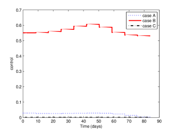
Figure 5.12: Bioeconomic approaches for optimal control

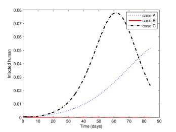
Figure 5.13: Bioeconomic approaches for infected humans

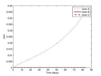
Figure 5.14: Bioeconomic approaches for total costs

In the medical perspective (case B), when only the costs related with ill people (absenteeism, drugs, …) are considered, the number of infected is the lowest; however a huge quantity of insecticide is used, because it is considered cheaper. On the other hand, when people just think on the economical perspective (case C), the treatment for people is neglected. Optimal control is low, but the number of infected humans is high. The total cost is higher when both perspectives are considered.

Epidemiological modelling has largely focused on identifying the mechanisms responsible for epidemics but has taken little account on economic constraints in analyzing control strategies. Economic models have given insight into optimal control under constraints imposed by limited resources, but they frequently ignore the spatial and temporal dynamics of the disease. Nowadays the combination of epidemiological and economic factors is essential. The bioeconomic approach requires an equilibrium between economic and epidemiological parameters in order to give an efficient disease control and reflecting the nature of the epidemic.

For this, the study goes on implementing both perspectives, but taking into account distinct weights of the parameters associated to the variables $i_{h}$ and $c$. Table 5.3 resumes these approaches.

	Bioeconomic perspective	Values for weights
		$\int_{0}^{t_{f}}\left[\gamma_{D}i_{h}(t)^{2}+\gamma_{S}c(t)^{2}\right]dt$
Case A	Both perspectives (equal weights)	$\gamma_{D}=0.5$; $\gamma_{S}=0.5$
Case D	Perspective centered in insecticide	$\gamma_{D}=0.2$; $\gamma_{S}=0.8$
Case E	Perspective centered in humans	$\gamma_{D}=0.8$; $\gamma_{S}=0.2$

Table 5.3: Different weights for the functional

In case D, it is studied a situation where the lack of insecticide in a country could be a reality and as a consequence its market value is high. This could happen due to an unprecedent outbreak where the authorities were not prepared or even due to financial reasons by the fact that the government does not have financial viability for this kind of measure. In case E, once again the human perspective gains strength and, as human life and quality of life is an expensive good, it was considered that it is more expensive to treat humans then apply insecticide.

The analysis from the Figures from 5.15 to 5.17 is consistent with what we expected in reality. In case D, as insecticide is expensive, the function for optimal control is lower than the other perspective. As consequence, the number of infected people is higher.

In case E, where the human factor is preponderant, the number of infected humans is low but expenses with insecticide are higher. Curiously the total cost, in case D and E, are of the same order of magnitude, with a slightly higher cost for case E. The total cost is reported in Table 5.4. When both perspectives are considered, the total cost is higher than the single perspective.

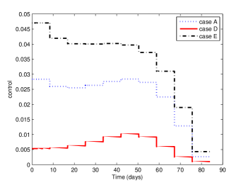
Figure 5.15: Optimal control, using different weights in the functional

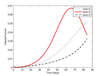
Figure 5.16: Infected human, using different weights in the functional

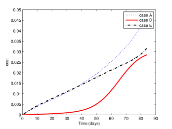
Figure 5.17: Total costs, using different weights in the functional

Case	Total cost
Case A	0.04700440
Case B	0.00000203
Case C	0.00004266
Case D	0.02852298
Case E	0.03172708

Table 5.4: Values for the functional in several cases

For a last analysis, a mathematical perspective was carried out: what values should the $\gamma_{D}$ and $\gamma_{S}$ have, in order to minimize the functional? Let us call this perspective as Case F. In this perspective, we not only want to minimize the control $c$, but also the parameters $\gamma_{D}$ and $\gamma_{S}$, enforcing the equality constraint $\gamma_{D}+\gamma_{S}=1$.

The values obtained from DOTcvp were $J=2.7\times 10^{-6}$, $\gamma_{D}=9.9962\times 10^{-1}$ and $\gamma_{S}=1.0863\times 10^{-10}$.

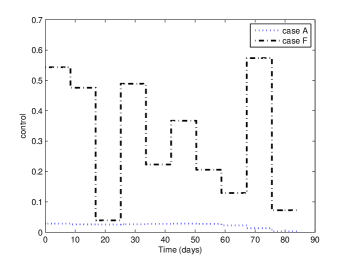
Figure 5.18: Comparison of optimal control, between initial and mathematical perspectives

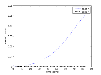
Figure 5.19: Comparison of infected humans, between initial and mathematical perspectives

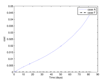
Figure 5.20: Comparison of total costs, between initial and mathematical perspectives

Figures 5.18 to 5.20 show the comparison of this case with the first one. As expected, the total cost and the number of infected humans are the lowest ones. Giving freedom to the parameters it is possible to see that the optimal control function is not periodic (as studied in the previous section), but gives a practical solution in applying insecticide.

5.4 Conclusions

In this chapter a model based on two populations, humans and mosquitoes, with insecticide control is presented. It has shown that as time goes by, depending on several parameters, the outbreak could disappear (leading to a DFE) or could transform the disease into an endemic one (leading to an EE). This analysis can be made through the threshold basic reproduction number.

Assuming that the parameters are fixed, the only variable that can influence this threshold is the control variable $c$, it has shown that with a steady insecticide campaign it is possible to reduce the number of infected humans and mosquitoes, and can prevent an outbreak that could transform an epidemiological episode to an endemic disease.

For a steady campaign has proven that $c=0.157$ it is enough to maintain the $\mathcal{R}_{0}$ below unit. However, this type of control is difficult to implement. A pulse insecticide campaign was studied to circumvent this difficulty. It has proven that applying insecticide every 6/7 days, is a better strategy to implement by health authorities and has the same efficacy level and financial costs.

Finally, the OC theory was used to find the best optimal control function for the insecticide. The optimal function varies, giving a different answer depending on the main goal to reach, thinking in economical or human centered perspective.

As future work it is important to study different kinds of controls. The accelerated increase in mosquito resistance to several chemical insecticides and the damage caused by these to the environment, has resulted in the search for new control alternatives. Among the alternatives available, the use of Bacillus thuringiensis israelensis (Bti) has been adopted by several countries [89]. Laboratory testing shows that Bti has a high larvicide property and its mechanism of action is based on the production of an endotoxin protein that, when ingested by the larvae, causes death. To ensure the minimization of the outbreaks, educational programmes that are customized for different levels of health care and that reflect local capacity should be supported and implemented widely. People should be instructed to minimize the number of potential places for the mosquito breeding. Educational campaigns can be included as an extra control parameter in the model.

This chapter was based on work available in the peer reviewed journal [118] and the peer reviewed conference proceedings [113, 117].

Chapter 6 An ODE SIR+ASI model with several controls

A new model with six mutually-exclusive compartments related to Dengue disease is presented. In this model there are three vector control tools: insecticides (larvicide and adulticide) and mechanical control. The human data for the model is again related to Cape Verde. Due to the rapid development of the outbreak on the islands, only a few control measures were taken, but not quantified. In this chapter, some of these measures are simulated and their consequences are analyzed.

 

In Chapter 5, a model with eight compartments and a single control was analyzed. However, after discussion with some researchers in this area, many of them suggested removing the compartment exposed for three main reasons: first, it is difficult to collect data for this compartment, since the disease at this stage does not show symptoms; second, the curve obtained is similar to the infected compartment with only an advance of time, not bringing novelty to the model, but possible difficulties to the numeric resolution; and finally, as the main goal is to study the effects of several controls centered in the infected humans, this compartment plays a secondary role. Thus, it was decided to remove the exposed compartments, in humans and mosquitoes, adjusting the other parameters to this new model and including three controls.

6.1 The SIR+ASI model

Taking into account the model presented in [43, 44] and the considerations of [111]-[113], a new model more adapted to the Dengue reality is proposed. The notation used in the mathematical model includes three epidemiological states for humans:

$S_{h}(t):$	susceptible
$I_{h}(t):$	infected
$R_{h}(t):$	resistant

It is assumed that the total human population $(N_{h})$ is constant and $N_{h}=S_{h}(t)+I_{h}(t)+R_{h}(t)$ at any time $t$. The population is homogeneous, which means that every individual of a compartment is homogeneously mixed with the other individuals. Immigration and emigration are not considered.

There are three other state variables, related to the female mosquitoes:

$A_{m}(t):$	aquatic phase
$S_{m}(t):$	susceptible
$I_{m}(t):$	infected

Due to the short lifespan of mosquitoes, there is no resistant phase. It is assumed homogeneity between host and vector populations, which means that each vector has an equal probability to bite any host. Humans and mosquitoes are assumed to be born susceptible.

To analyze the effect of campaigns in the disease fight, three controls are considered:

$c_{A}(t):$	proportion of larvicide, $0\leq c_{A}\leq 1$
$c_{m}(t):$	proportion of adulticide, $0\leq c_{m}\leq 1$
$\alpha(t):$	proportion of mechanical control, $0<\alpha\leq 1$.

Larval control targets the immature mosquitoes living in water before they become biting adults. A soil bacterium, Bacillus thuringiensis israelensis (Bti), is applied from the ground or by air to larval habitats. This bacterium is used because when properly applied, it has virtually no effect on non-target organisms.

The control of adult mosquitoes is necessary when mosquito populations cannot be treated in their larval stage. It is the most effective way to eliminate adult female mosquitoes that are infected with human pathogens. Depending on the size of the area to be treated, either trucks for ground adulticide treatments or aircraft for aerial adulticide treatments can be used.

The purpose of mechanical control is to reduce the number of larval habitat areas available to mosquitoes. The mosquitoes are most easily controlled by treating, cleaning and/or emptying containers that hold water, since the eggs of the specie are laid in water-holding containers.

The aim is to simulate different realities in order to find the best policy to decrease the number of infected humans. A temporal mathematical model is introduced, with mutually-exclusive compartments, to study the outbreak occurred on Cape Verde islands in 2009 and improving the model described in [111].

The model uses the following parameters:

$N_{h}:$	total population
$B:$	average daily biting (per day)
$\beta_{mh}:$	transmission probability from $I_{m}$ (per bite)
$\beta_{hm}:$	transmission probability from $I_{h}$ (per bite)
$1/\mu_{h}:$	average lifespan of humans (in days)
$1/\eta_{h}:$	mean viremic period (in days)
$1/\mu_{m}:$	average lifespan of adult mosquitoes (in days)
$\varphi:$	number of eggs at each deposit per capita (per day)
$1/\mu_{A}:$	natural mortality of larvae (per day)
$\eta_{A}:$	maturation rate from larvae to adult (per day)
$m:$	female mosquitoes per human
$k:$	number of larvae per human

The Dengue epidemic is modelled by the following nonlinear time-varying state equations:

$$\begin{cases}\displaystyle\frac{dS_{h}}{dt}=\mu_{h}N_{h}-\left(B\beta_{mh}\frac{I_{m}}{N_{h}}+\mu_{h}\right)S_{h}\\ \displaystyle\frac{dI_{h}}{dt}=B\beta_{mh}\frac{I_{m}}{N_{h}}S_{h}-(\eta_{h}+\mu_{h})I_{h}\\ \displaystyle\frac{dR_{h}}{dt}=\eta_{h}I_{h}-\mu_{h}R_{h}\end{cases}$$ (6.1)

and

$$\begin{cases}\displaystyle\frac{dA_{m}}{dt}=\varphi\left(1-\frac{A_{m}}{\alpha kN_{h}}\right)(S_{m}+I_{m})-\left(\eta_{A}+\mu_{A}+c_{A}\right)A_{m}\\ \displaystyle\frac{dS_{m}}{dt}=\eta_{A}A_{m}-\left(B\beta_{hm}\frac{I_{h}}{N_{h}}+\mu_{m}+c_{m}\right)S_{m}\\ \displaystyle\frac{dI_{m}}{dt}=B\beta_{hm}\frac{I_{h}}{N_{h}}S_{m}-\left(\mu_{m}+c_{m}\right)I_{m}\end{cases}$$ (6.2)

with the initial conditions

$$S_{h}(0)=S_{h0},$$

Figure 6.1 shows a scheme of the model.

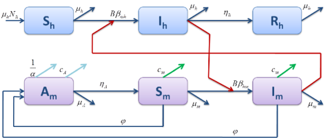
Figure 6.1: Epidemiological model SIR + ASI

Basic reproduction number, equilibrium points and stability

Due to biological reasons, only nonnegative solutions of the differential system are acceptable. More precisely, it is necessary to study the solution properties of the system (6.1)–(6.2) in the closed set

$$\Omega=\left\{(S_{h},I_{h},R_{h},A_{m},S_{m},I_{m})\in\mathbb{R}_{+}^{6}:S_{h}+I_{h}+R_{h}\leq N_{h},\,A_{m}\leq kN_{h},\,S_{m}+I_{m}\leq mN_{h}\right\}.$$

It can be verified that $\Omega$ is a positively invariant set with respect to (6.1)–(6.2). The proof of this statement is similar as in [118]. The system (6.1)–(6.2) has at most three biologically meaningful equilibrium points (cf. Theorem 6.1.1).

Definition 18 (Equilibrium points for SIR+ASI model).

A sextuple $E=\left(S_{h},I_{h},R_{h},A_{m},S_{m},I_{m}\right)$ is said to be an equilibrium point for system (6.1)–(6.2) if it satisfies the following relations:

$$\begin{cases}\mu_{h}N_{h}-\left(B\beta_{mh}\frac{I_{m}}{N_{h}}+\mu_{h}\right)S_{h}=0\\ B\beta_{mh}\frac{I_{m}}{N_{h}}S_{h}-(\eta_{h}+\mu_{h})I_{h}=0\\ \eta_{h}I_{h}-\mu_{h}R_{h}=0\\ \varphi\left(1-\frac{A_{m}}{\alpha kN_{h}}\right)(S_{m}+I_{m})-(\eta_{A}+\mu_{A}+c_{A})A_{m}=0\\ \eta_{A}A_{m}-\left(B\beta_{hm}\frac{I_{h}}{N_{h}}+\mu_{m}+c_{m}\right)S_{m}=0\\ B\beta_{hm}\frac{I_{h}}{N_{h}}S_{m}-(\mu_{m}+c_{m})I_{m}=0.\end{cases}$$ (6.3)

An equilibrium point $E$ is biologically meaningful if and only if $E\in\Omega$. The biologically meaningful equilibrium points are said to be disease free or endemic depending on $I_{h}$ and $I_{m}$: if there is no disease for both populations of humans and mosquitoes ($I_{h}=I_{m}=0$), then the equilibrium point is said to be a Disease Free Equilibrium (DFE); otherwise, if $I_{h}\neq 0$ or $I_{m}\neq 0$ (in other words, if $I_{h}>0$ or $I_{m}>0$), then the equilibrium point is called endemic.

Theorem 6.1.1.

System (6.1)–(6.2) admits at most three biologically meaningful equilibrium points; at most two DFE points and at most one endemic equilibrium point. More precisely, let

$$\mathcal{M}=-\left(\eta_{A}\mu_{m}+\eta_{A}c_{m}+\mu_{A}\mu_{m}+\mu_{A}c_{m}+c_{A}\mu_{m}+c_{A}c_{m}-\varphi\eta_{A}\right),$$

$$\xi=\varphi(\mu_{m}+c_{m})^{2}(\eta_{h}+\mu_{h}),\quad\chi=\alpha kB^{2}\beta_{hm}\beta_{mh}\mathcal{M},$$

$$E_{1}^{*}=\left(N_{h},0,0,0,0,0\right),\quad E_{2}^{*}=\left(N_{h},0,0,\frac{\alpha kN_{h}\mathcal{M}}{\eta_{A}\varphi},\frac{\alpha kN_{h}\mathcal{M}}{(\mu_{m}+c_{m})\varphi},0\right),$$

and $E_{3}^{*}=\left(S_{h}^{*},I_{h}^{*},R_{h}^{*},A_{m}^{*},S_{m}^{*},I_{m}^{*}\right)$ with

$$\begin{split}S_{h}^{*}&=\frac{-\varphi N_{h}(\mu_{m}\eta_{h}+\mu_{h}B\beta_{hm}+c_{m}\mu_{h}+c_{m}\eta_{h}+\mu_{m}\mu_{h})(\mu_{m}+c_{m})}{B\beta_{hm}(-\alpha kB\beta_{mh}\mathcal{M}-\varphi\mu_{h}(\mu_{m}+c_{m}))},\\ I_{h}^{*}&=\frac{\mu_{h}N_{h}\left(\xi-\chi\right)}{(\eta_{h}+\mu_{h})B\beta_{hm}(-\alpha kB\beta_{mh}\mathcal{M}-\varphi\mu_{h}(\mu_{m}+c_{m}))},\\ R_{h}^{*}&=\frac{\eta_{h}N_{h}\left(\xi-\chi\right)}{(\eta_{h}+\mu_{h})B\beta_{hm}\left(-\alpha kB\beta_{mh}\mathcal{M}-\varphi\mu_{h}(\mu_{m}+c_{m})\right)},\\ A_{m}^{*}&=\frac{N_{h}k\alpha\mathcal{M}}{\varphi\eta_{A}},\\ S_{m}^{*}&=\frac{N_{h}\mu_{h}(c_{m}+\mu_{h})(\mu_{h}+\eta_{h})}{B\beta_{mh}(\mu_{m}\eta_{h}+\mu_{h}B\beta_{hm}+c-m\mu_{h}+c_{m}\eta_{h}+\mu_{m}\mu_{h})}\\ &\qquad-\frac{N_{h}\alpha k\left(c_{m}(\mu_{h}+\eta_{h})(\mu_{A}+\eta_{A}+c_{A})+\mu_{m}(\mu_{h}(\eta_{A}+\mu_{A})+\eta_{h}(c_{A}+\eta_{A}))\right)}{\varphi(\mu_{m}\eta_{h}+\mu_{h}B\beta_{hm}+c-m\mu_{h}+c_{m}\eta_{h}+\mu_{m}\mu_{h})}\\ &\qquad-\frac{N_{h}\alpha k\left(-\eta\varphi(\mu_{h}+\eta_{h})+\mu_{m}(\eta_{h}\mu_{A}+\mu_{h}c_{A})\right)}{\varphi(\mu_{m}\eta_{h}+\mu_{h}B\beta_{hm}+c-m\mu_{h}+c_{m}\eta_{h}+\mu_{m}\mu_{h})},\\ I_{m}^{*}&=\frac{-\mu_{h}N_{h}\left(\xi-\chi\right)}{B\beta_{mh}\left(\varphi B\beta_{hm}\mu_{h}(\mu_{m}+c_{m})+\xi\right)}.\end{split}$$ (6.4)

If $\mathcal{M}\leq 0$, then there is only one biologically meaningful equilibrium point, $E_{1}^{*}$, which is a DFE point. If $\mathcal{M}>0$ with $\xi\geq\chi$, then there are two biologically meaningful equilibrium points, $E_{1}^{*}$ and $E_{2}^{*}$, both DFE points. If $\mathcal{M}>0$ with $\xi<\chi$, then there are three biologically meaningful equilibrium points, $E_{1}^{*}$, $E_{2}^{*}$, and $E_{3}^{*}$, where $E_{1}^{*}$ and $E_{2}^{*}$ are DFEs and $E_{3}^{*}$ endemic.

Proof.

System (6.3) has four solutions easily obtained with a Computer Algebra System like Maple: $E_{1}^{*}$, $E_{2}^{*}$, $E_{3}^{*}$ and $E_{4}^{*}$. The equilibrium point $E_{1}^{*}$ is always a DFE because it always belongs to $\Omega$ with $I_{h}=I_{m}=0$. In contrast, $E_{4}^{*}$ is never biologically realistic because it has always some negative coordinates. The other two equilibrium points, $E_{2}^{*}$ and $E_{3}^{*}$, are biologically realistic only for certain values of the parameters. The equilibrium $E_{2}^{*}$ is biologically realistic if and only if $\mathcal{M}\geq 0$, in which case it is a DFE. For the condition $\mathcal{M}\leq 0$, the third equilibrium $E_{3}^{*}$ is not biologically realistic. If $\mathcal{M}>0$, then three situations can occur with respect to $E_{3}^{*}$: if $\xi=\chi$, then $E_{3}^{*}$ degenerates into $E_{2}^{*}$, which means that $E_{3}^{*}$ is the DFE $E_{2}^{*}$; if $\xi>\chi$, then $E_{3}^{*}$ is not biologically realistic; otherwise, one has $E_{3}^{*}\in\Omega$ with $I_{h}\neq 0$ and $I_{m}\neq 0$, which means that $E_{3}^{*}$ is an endemic equilibrium point. ∎

By algebraic manipulation, $\mathcal{M}>0$ is equivalent to condition $\displaystyle\frac{(\eta_{A}+\mu_{A}+c_{A})(\mu_{m}+c_{m})}{\varphi\eta_{A}}>1$, which is related to the basic offspring number for mosquitos. Thus, if $\mathcal{M}\leq 0$, then the mosquito population will collapse and the only equilibrium for the whole system is the trivial DFE $E_{1}^{*}$. If $\mathcal{M}>0$, then the mosquito population is sustainable. From a biological standpoint, the equilibrium $E_{2}^{*}$ is more plausible, because the mosquito is in its habitat, but without the disease.

An important measure of transmissibility of the disease is now introduced: the basic reproduction number. It provides an invasion criterion for the initial spread of the virus in a susceptible population. For this case the following result holds.

Theorem 6.1.2.

The basic reproduction number $\mathcal{R}_{0}$ associated to the differential system (6.1)–(6.2) is

$$\mathcal{R}_{0}=\left(\frac{\alpha kB^{2}\beta_{hm}\beta_{mh}\mathcal{M}}{\varphi(\eta_{h}+\mu_{h})(c_{m}+\mu_{m})^{2}}\right)^{\frac{1}{2}}=\left(\frac{\chi}{\xi}\right)^{\frac{1}{2}}.$$ (6.5)

Proof.

In agreement with [42], just the epidemiological compartments that have new infections, $I_{h}$ and $I_{m}$, are considered. The two differential equations related to these two compartments can be rewritten as $\dfrac{dx}{dt}=\mathcal{F}-\mathcal{V}$, where $\mathcal{F}$ is the rate of production of new infections and $\mathcal{V}$ is the transition rates between states:

$$\mathcal{F}(x)=\left(\begin{array}[]{c}B\beta_{mh}\frac{I_{m}}{N_{h}}S_{h}\\ B\beta_{hm}\frac{I_{h}}{N_{h}}S_{m}\\ \end{array}\right),\quad\mathcal{V}(x)=\left(\begin{array}[]{c}(\eta_{h}+\mu_{h})I_{h}\\ (c_{m}+\mu_{m})I_{m}\\ \end{array}\right).$$

The Jacobian derivatives are

$$J_{\mathcal{F}(x)}=\left(\begin{array}[]{cc}0&B\beta_{mh}\frac{S_{h}}{N_{h}}\\ B\beta_{hm}\frac{S_{m}}{N_{h}}&0\\ \end{array}\right),\quad J_{\mathcal{V}(x)}=\left(\begin{array}[]{cc}(\eta_{h}+\mu_{h})&0\\ 0&(c_{m}+\mu_{m})\\ \end{array}\right).$$

The quantity $J_{\mathcal{F}(x)}J_{\mathcal{V}(x)}^{-1}$ gives the total production of new infections over the course of an infection. The largest eigenvalue gives the fastest growth of the infected population, which means that $\mathcal{R}_{0}$ is the spectral radius of the matrix $J_{\mathcal{F}(x)}J_{\mathcal{V}(x)}^{-1}$ in a DFE point. Maple was used to obtain

$$\mathcal{R}_{0}=\left(\frac{B^{2}\beta_{hm}\beta_{mh}S_{h_{DFE}}S_{m_{DFE}}}{(\eta_{h}+\mu_{h})(c_{m}+\mu_{m})N_{h}^{2}}\right)^{\frac{1}{2}}.$$ (6.6)

The basic reproduction number $\mathcal{R}_{0}$ in (6.5) is obtained, replacing $S_{h_{DFE}}$ and $S_{m_{DFE}}$ in (6.6) by those of the DFE $E_{2}^{*}$. ∎

The model has two different populations (host and vector) and the expected basic reproduction number should reflect the infection transmitted from host to vector and vice-versa. Accordingly, $\mathcal{R}_{0}$ can be seen as $\mathcal{R}_{0}=(\mathcal{R}_{hm}\times\mathcal{R}_{mh})^{\frac{1}{2}}$. The infection host-vector is represented by $\mathcal{R}_{hm}=\frac{B\beta_{hm}S_{m_{DFE}}}{N_{h}(\eta_{h}+\mu_{h})}$, where the term $\frac{B\beta_{hm}S_{m_{DFE}}}{N_{h}}$ represents the product between the transmission probability of the disease from humans to mosquitoes in a susceptible population of vectors, and the term $\frac{1}{\eta_{h}+\mu_{h}}$ the human viremic period. Analogously, the infection vector-host is composed by $\mathcal{R}_{mh}=\frac{B\beta_{mh}S_{h_{DFE}}}{N_{h}(c_{m}+\mu_{m})}$, where $\frac{B\beta_{mh}S_{h_{DFE}}}{N_{h}}$ describes the transmission of the disease from mosquito to the susceptible human population, and $\frac{1}{c_{m}+\mu_{m}}$ the lifespan of an adult mosquito.

If $\mathcal{R}_{0}<1$, then, on average, an infected individual produces less than one new infected individual over the course of its infectious period, and the disease cannot grow. Conversely, if $\mathcal{R}_{0}>1$, then each individual infects more than one person, and the disease can invade the population.

Theorem 6.1.3.

If $\mathcal{M}>0$ and $\mathcal{R}_{0}>1$, then the system (6.1)–(6.2) admits the endemic equilibrium $E_{3}^{*}=\left(S_{h}^{*},I_{h}^{*},R_{h}^{*},A_{m}^{*},S_{m}^{*},I_{m}^{*}\right)$ given by (6.4).

Proof.

The only solution of (6.3) with $I_{h}>0$ or $I_{m}>0$, the only endemic equilibrium, is $E_{3}^{*}$. That occurs, in agreement with Theorem 6.1.1, in the case $\mathcal{M}>0$ and $\chi>\xi$. The condition $\chi>\xi$ is equivalent, by Theorem 6.1.2, to $\mathcal{R}_{0}>1$. ∎

Using the methods in [42, 83], it is possible to prove that if $\mathcal{R}_{0}\leq 1$, then the DFE is globally asymptotically stable in $\Omega$, and thus the vector-borne disease always dies out; if $\mathcal{R}_{0}>1$, then the unique endemic equilibrium is globally asymptotically stable in $\Omega$, so that the disease, if initially present, will persist at the unique endemic equilibrium level.

Assuming that parameters are fixed, the threshold $\mathcal{R}_{0}$ is influenceable by the control values. Figure 6.2 gives this relationship. It is possible to realize that the control $c_{m}$ is the one that most influences the basic reproduction number to stay below unit. Besides, the control in the aquatic phase alone is not enough to maintain $\mathcal{R}_{0}$ below unit: an application close to 100% is required.

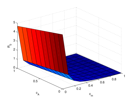
(a) $\mathcal{R}_{0}$ as a function of $c_{m}$ and $c_{A}$

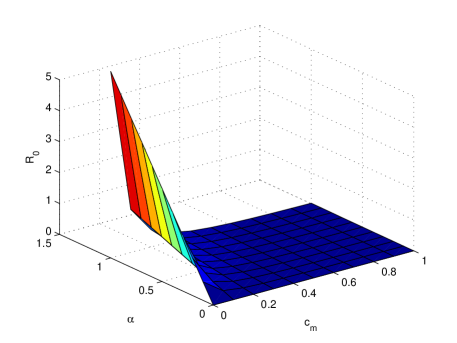
(b) $\mathcal{R}_{0}$ as a function of $c_{m}$ and $\alpha$

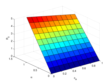
(c) $\mathcal{R}_{0}$ as a function of $c_{A}$ and $\alpha$

Figure 6.2: Influence of the controls on the basic reproduction number $\mathcal{R}_{0}$

6.2 Numerical implementation

The simulations were carried out using the following numerical values: $N_{h}=480000$, $B=0.8$, $\beta_{mh}=0.375$, $\beta_{hm}=0.375$, $\mu_{h}=1/(71\times 365)$, $\eta_{h}=1/3$, $\mu_{m}=1/10$, $\varphi=6$, $\mu_{A}=1/4$, $\eta_{A}=0.08$, $m=3$, $k=3$. The initial conditions for the problem were: $S_{h0}=N_{h}-10$, $I_{h0}=10$, $R_{h0}=0$, $A_{m0}=kN_{h}$, $S_{m0}=mN_{h}$, $I_{m0}=0$. With these values, one has $\mathcal{M}>0$. As in the previous chapter the values related to humans describe the reality of Cape Verde [32] and the information about mosquitoes is based on Brazil [30, 47].

All computational calculus consider one year for time interval. Although the final time was $t_{f}=365$ days, the figures show graphics in suitable windows, in order to provide a better analysis. All the simulations and graphics were done in Matlab. To solve the differential equation system, the ode45 routine was used. This function implements a Runge-Kutta method with a variable time step for efficient computation (see [110] for more details about the code).

Figures 6.3 and 6.4 describe the human and mosquito populations in the absence of any control, respectively. The number of human infection has a peak between the 30th and the 40th day. The infection of the mosquitoes had a delay when compared to the humans.

The number of infected humans from the model (6.1)–(6.2) is higher when compared with what really happened in Cape Verde. As far as it was possible to investigate in the local news, the government of Cape Verde has done their best to banish the mosquito, with media campaigns appealing to people to remove or cover all recipients that could serve to breed the mosquito, and to use insecticide in critical areas. However, it was not possible to quantify those efforts in precise terms.

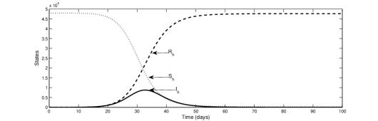
Figure 6.3: Human population (without control)

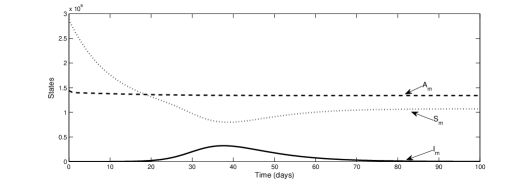
Figure 6.4: Mosquito population (without control)

Next, follows a set of simulations using different controls. In each figure, only one control is used, continuously, which means that the others are not applied. The aim of this simulation is to see the importance of the control and what repercussions has on the model. Figures 6.5 and 6.6 concern the adulticide control, Figures 6.7 and 6.8 the larvicide control, and Figures 6.9 and 6.10 the mechanical control. Using a small quantity of each control, the number of infected people falls dramatically. In some cases, in spite of all graphs displaying five simulations, some curves are so close to zero that it is difficult to distinguish them.

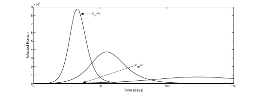
Figure 6.5: Infected humans using different levels of adulticide ($c_{m}=0$, 0.25, 0.50, 0.75, 1)

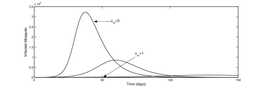
Figure 6.6: Infected mosquitoes with different levels of adulticide ($c_{m}=0$, 0.25, 0.50, 0.75, 1)

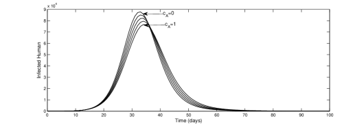
Figure 6.7: Infected humans using different levels of larvicide ($c_{A}=0$, 0.25, 0.50, 0.75, 1)

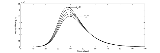
Figure 6.8: Infected mosquitoes using different levels of larvicide ($c_{A}=0$, 0.25, 0.50, 0.75, 1)

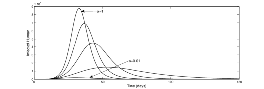
Figure 6.9: Infected humans using different levels of mechanical control ($\alpha=0.01$, 0.25, 0.5, 0.75, 1)

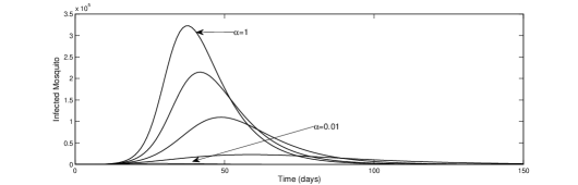
Figure 6.10: Infected mosquitoes using different levels of mechanical control ($\alpha=0.01$, 0.25, 0.5, 0.75, 1)

Figures 6.5 and 6.6 show that excellent results for the human population are obtained by covering only 25% of the country with insecticide for adult mosquitoes. The simulations were done considering that the aedes aegypti does not become resistant to the insecticide and that it is financially possible to apply insecticide during all time. Figures 6.7–6.10 are related to the applied controls in the aquatic phase of the mosquito. In these graphics the controls were studied separately, but one is closely related to the other. The application of these controls are not sufficient to decrease the infected human to zero, but the removal of breeding sites and the use of larvicide is important to the reduction of that number.

Figures 6.11 and 6.12 show several simulations using three controls at different levels, simultaneously. Only $10\%$ of each control, applied continuously, is enough for the number of infected, humans and mosquitoes, to remain near zero.

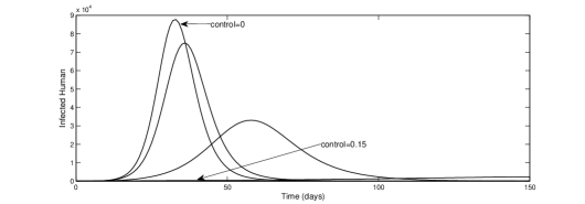
Figure 6.11: Infected humans using different levels of control ($c_{A}=c_{m}=1-\alpha=0$, 0.01, 0.05, 0.1, 0.15)

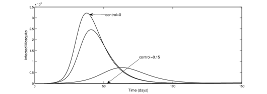
Figure 6.12: Infected mosquitoes using different levels of control ($c_{A}=c_{m}=1-\alpha=0$, 0.01, 0.05, 0.1, 0.15)

In the next section, using OC strategy we will find the best solution for the controls.

6.3 Optimal control with several controls

Epidemiological models may give some basic guidelines for public health practitioners, comparing the effectiveness of different potential management strategies.

In reality, a range of constraints and trade-offs may substantially influence the choice of practical strategy, and therefore their inclusion in any modelling analysis may be important. Frequently, epidemiological models need to be coupled to economic considerations, such that control strategies can be judged through holistic cost-benefit analysis. Control of livestock disease is a scenario when cost-benefit analysis can play a vital role in choosing between cheap, weak controls that lead to a prolonged epidemic, or expensive but more effective controls that lead to a shorter outbreak.

Normalizing the previous ODE system (6.1)–(6.2), we obtain:

$$\begin{cases}\dfrac{ds_{h}}{dt}=\mu_{h}-\left(B\beta_{mh}mi_{m}+\mu_{h}\right)s_{h}\\ \dfrac{di_{h}}{dt}=B\beta_{mh}mi_{m}s_{h}-(\eta_{h}+\mu_{h})i_{h}\\ \dfrac{dr_{h}}{dt}=\eta_{h}i_{h}-\mu_{h}r_{h}\\ \dfrac{da_{m}}{dt}=\varphi\frac{m}{k}\left(1-\frac{a_{m}}{\alpha}\right)(s_{m}+i_{m})-\left(\eta_{A}+\mu_{A}+c_{A}\right)a_{m}\\ \dfrac{ds_{m}}{dt}=\eta_{A}\frac{k}{m}a_{m}-\left(B\beta_{hm}i_{h}+\mu_{m}+c_{m}\right)s_{m}\\ \dfrac{di_{m}}{dt}=B\beta_{hm}i_{h}s_{m}-\left(\mu_{m}+c_{m}\right)i_{m}\end{cases}$$ (6.7)

with the initial conditions

$$s_{h}(0)=0.9999,$$

(6.8)

The cost functional considered was

minimize $$J\left(u_{1}(\cdot),u_{2}(\cdot)\right)=\int_{0}^{t_{f}}\left[\gamma_{D}i_{h}(t)^{2}+\gamma_{S}c_{m}(t)^{2}+\gamma_{L}c_{A}(t)^{2}+\gamma_{E}\left(1-\alpha\right)^{2}\right]dt$$

(6.9)

where $\gamma_{D}$, $\gamma_{S}$, $\gamma_{L}$ and $\gamma_{E}$ are weights related to costs of the disease, adulticide, larvicide and mechanical control, respectively.

In a first approach to this problem, it is assumed that all weights are the same, which means $\gamma_{D}=\gamma_{S}=\gamma_{L}=\gamma_{E}=0.25$ (Case A).

The OC problem was solved using two different packages: DOTcvp [67] and Muscod-II [79]. The mathematical formulation of the SIR+ASI problem, for the both packages, is available on [110]. The simulation behavior is similar, and we decided to show only the DOTcvp results. The optimal functions for the controls are given in Figure 6.16.

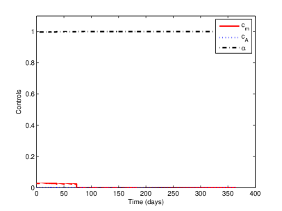
Figure 6.13: Optimal control functions (Case A: $\gamma_{D}=\gamma_{S}=\gamma_{L}=\gamma_{E}=0.25$)

The adulticide was the control that more influenced the decreasing of that ratio and, as consequence, the decreasing of the number of infected people and mosquitoes, matching with the results obtained for the basic reproduction number in Section 6.1. Therefore, the adulticide was the most used. We believe that the other controls do not assume an important role in the epidemic episode, because all the events happened at a short period of time, which means that adulticide has more impact. However the mosquito control in the aquatic phase can not be neglected. In situations of longer epidemic episodes or even in an endemic situation, the larval control represents an important tool.

Figure 6.14 presents the number of infected humans. Comparing the optimal control case with a situation with no control, the number of infected people decreased considerably. Besides, in the situation where OC is used, the peak of infected people is minor, which facilitates the work in health centers, because they can provide a better medical monitoring.

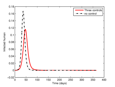
Figure 6.14: Comparison of infected individuals under an optimal control situation and no controls

A second analysis was made, taking into account different weights on the functional. Table 6.1 resumes the weights chosen for perspectives: not only economic issues (cost of insecticides and educational campaigns), but also human issues are considered. In case A, all costs were equal. In case B is given more impact on the infected people, considering that the treatment and absenteeism to work is very prejudicial to the country, when compared with the cost of insecticides and educational campaigns. In case C, the costs with killing mosquitoes and educational campaigns have more impact in the economy. Higher total costs were obtained when human life had more weight than controls measures as can be checked in Table 6.1.

	Values for weights	Cost obtained
Case A	$\gamma_{D}=0.25$; $\gamma_{S}=0.25$; $\gamma_{L}=0.25$; $\gamma_{E}=0.25$	0.06691425
Case B	$\gamma_{D}=0.55$; $\gamma_{S}=0.15$; $\gamma_{L}=0.15$; $\gamma_{E}=0.15$	0.10431186
Case C	$\gamma_{D}=0.10$; $\gamma_{S}=0.30$; $\gamma_{L}=0.30$; $\gamma_{E}=0.30$	0.03012849

Table 6.1: Different weights for the functional and respective values

Figure 6.15 shows the number of infected human in each bioeconomic perspective. We can realize that Case A and Case C are similar. It can be explained by the low weight given to the cost of treatment (cases A and C) when compared with the heavy weight given in case B. Figure 6.16 presents the behavior of the controls for the A, B and C cases. Again, as adulticide is the one that has more influence on the model, this is the control that most varies when the weights are changed.

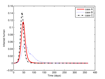
Figure 6.15: Infected individuals in three bioeconomic perspectives

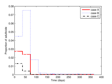
(a) Adulticide

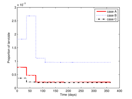
(b) Larvicide

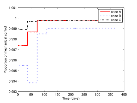
(c) Mechanical control

Figure 6.16: Proportion of control used in the three bioeconomic perspective

A third analysis was made to the model: it changed the functional in order to study the effects of each control when separately considered. Therefore, the new functional also considers bioeconomic perspectives, but only includes two variables: the costs with infected humans (with $\gamma_{D}=0.5$) and the costs with only one control (with $\gamma_{i}=0.5,i\in\{S,L,E\}$). Thus, in Figure 6.17 are presented the proportion of adulticide $(a)$ and infected humans $(b)$, when the functional is $\int_{0}^{t_{f}}\left[\gamma_{D}i_{h}(t)^{2}+\gamma_{S}c_{m}(t)^{2}\right]dt$. Figures 6.18 and 6.19 represent the same simulations when the controls considered are larvicide and mechanical control, respectively. It is possible to see that the use of larvicide and mechanical control, used alone, does not bring relevant influence on the control of the disease.

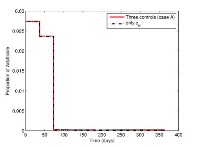
(a) Optimal control $c_{m}$

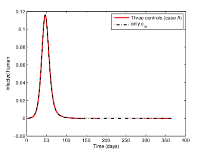
(b) Proportion of infected human

Figure 6.17: Optimal control and infected humans when considered all controls (solid line) and only adulticide control (dashed line) in one year

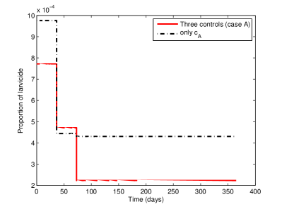
(a) Optimal control $c_{A}$

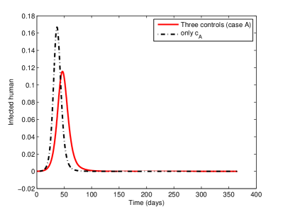
(b) Proportion of infected human

Figure 6.18: Optimal control and infected humans when considered all controls (solid line) and only larvicide control (dashed line) in one year

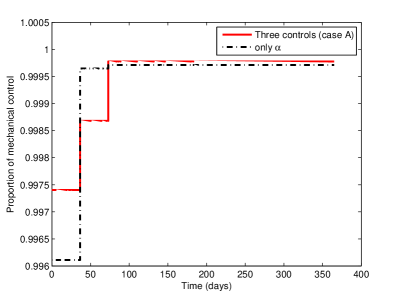
(a) Optimal control $\alpha$

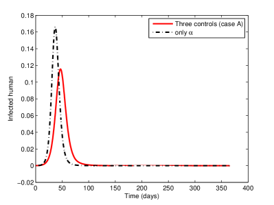
(b) Proportion of infected human

Figure 6.19: Optimal control and infected humans when considered all controls (solid line) and only mechanical control (dashed line) in one year

6.4 Conclusions

Dengue disease breeds, even in the absence of fatal forms, significant economic and social costs: absenteeism, debilitation and medication. To observe and to act at the epidemics onset could save lives and resources to governments. Moreover, the under-reporting of Dengue cases is probably the most important barrier in obtaining an accurate assessment.

A compartmental epidemiological model for Dengue disease composed by a set of differential equations was presented. Simulations based on clean-up campaigns to remove the vector breeding sites, and also simulations on the application of insecticides (larvicide and adulticide), were made. It was shown that even with a low, although continuous, index of control over time, the results are surprisingly positive. The adulticide was the most effective control, since with a low percentage of insecticide, the basic reproduction number is kept below unit and the number infected humans was smaller. However, to bet only in adulticide is a risky decision. In some countries, such as Mexico and Brazil, the prolonged use of adulticides has been increasing the mosquito tolerance capacity to the product or even they become completely resistant. In countries where Dengue is a permanent threat, governments must act with differentiated tools. It will be interesting to analyze these controls in an endemic region and with several outbreaks. We believe that the results will be quite different. Aedes aegypti eradication is not considered to be feasible and, from the environmental point of view, not desirable. The aim is to reduce the mosquito density and, simultaneously, amount the level of immunity on the human population. The increase of population herd immunity can be reached by two ways: increasing the resistant people to the disease implying an increasing of infected individuals or with a vaccination campaign. No commercially available clinical cure or vaccine is currently available for Dengue, but efforts are underway to develop one [10, 68]. The potential of prevention of Dengue by immunization seems to be technically feasible and progress is being made in the development of vaccines that may protect against all four Dengue viruses. In the next chapter, a model of this disease with a vaccine simulation as a new strategy to fight the disease will be analyzed.

This chapter was based on work accepted in the peer reviewed journal [115] and the peer reviewed conference proceedings [116].

Chapter 7 Dengue with vaccine simulations

As the development of a Dengue vaccine is ongoing, it is simulated an hypothetical vaccine as an extra protection to the population. In a first phase, the vaccination process is studied as a new compartment in the model, and some different types of vaccines are simulated: pediatric and random mass vaccines, with distinct levels of efficacy and durability. In a second step, the vaccination is seen as a control variable in the epidemiological process. In both cases, epidemic and endemic scenarios are included in order to analyze distinct outbreak realities.

 

In 1760, the Swiss mathematician Daniel Bernoulli published a study on the impact of immunization with cowpox upon the expectation of life of the immunized population [119]. The process of protecting individuals from infection by immunization has become a routine, with historical success in reducing both mortality and morbidity.

The impact of vaccination may be regarded not only as an individual protective measure, but also as a collective one. While direct individual protection is the major focus of a mass vaccination program, the effects on population also contribute indirectly to other individual protection through herd immunity, providing protection for unprotected individuals [48] (see scheme in Figure 7.1). This means that when we have a large neighborhood of vaccinated people, a susceptible individual has a lower probability in coming into contact with the infection, being more difficult for diseases to spread, which decreases the relief of health facilities and can break the chain of infection.

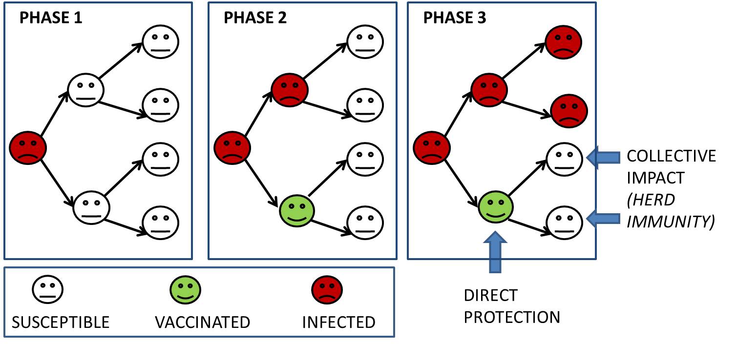
Figure 7.1: Individual and collective protection provided from a vaccination campaign

7.1 About Dengue vaccine

Vector control remains the only available strategy against Dengue. Despite integrated vector control with community participation, along with active disease surveillance and insecticides, there are only a few examples of successful Dengue prevention and control on a national scale [23]. Besides, the levels of resistance of Aedes aegypti to insecticides has increased, which implies shorter intervals between treatments, and only few insecticide products are available in the market due to the high costs for development and registration and low returns [76].

Dengue vaccines have been under development since the 1940s, but due to the limited appreciation of global disease burden and the potential markets for Dengue vaccines, industry interest languished throughout the 20th century. However, in recent years, the development of Dengue vaccines has accelerated dramatically with the increase in Dengue infections, as well as the prevalence of all four circulating serotypes. Faster development of a vaccine became a serious concern [94].

Economic analysis are now conducted periodically to guide public support for vaccine development in both industrialized and developing countries, including a previous cost-effectiveness study of Dengue [28, 123, 126]. The authors compared the cost of the disease burden with the possibility of making a vaccination campaign; they suggest that there is a potential economic benefit associated with promising Dengue interventions, such as Dengue vaccines and vector control innovations, when compared to the cost associated to the disease treatments.

Constructing a successful vaccine for Dengue has been challenging: the knowledge of disease pathogenesis is insufficient and in addition the vaccine must protect simultaneously against all serotypes in order to not increase the level of DHF [128].

Nevertheless, several promising approaches are being investigated in both academic and industrial laboratories. Vaccine candidates include live attenuated vaccines obtained via cell passages or by recombinant DNA technology (such as those being developed by the US National Institutes of Allergy and Infectious Diseases, InViragen, Walter Reed Army Institute of Research/GlaxoSmithKline, and Sanofi Pasteur) and subunit vaccines (such as those developed by Merck/Hawaii Biotech) [60, 138]. Recent studies indicate that, by the progress in clinical development of Sanofi Pasteur’s live attenuated tetravalent chimeric vaccine, a vaccine could be licensed as early as 2014 [87]. The team is carrying out an efficacy study on a vaccine covering four serotypes on 4000 children aged four to eleven years old in Muang district, Thailand.

At this time, the features of Dengue vaccine are mostly unknown. So, in this chapter we opt to present a set of simulations with different types of vaccines and we have explored also the vaccination process under two different perspectives. The first one uses a new compartment in the model and several kinds of vaccination are considered. A second perspective is studied using the vaccination process as a disease control in the mathematical formulation. In this case the theory of OC is applied. Both methods assume a continuous strategy vaccination.

7.2 Vaccine as a new compartment

In this section, a new compartment $V$ is added to the previous $SIR$ model related to the human population. This new compartment represents the new group of human population that is vaccinated, in order to distinguish the resistance obtained through vaccination and the one achieved by disease recovery.

Two forms of random vaccination are possible: the most common for human disease is pediatric vaccination to reduce the prevalence of an endemic disease; the alternative is random vaccination of the entire population in an outbreak situation. In both types, the vaccination can be considered perfect conferring 100% protection for all life or else imperfect. This last case can be due to the difficulty of producing an effective vaccine, the heterogeneity of the population or even the life span of the vaccine.

7.2.1 Perfect pediatric vaccine

For many potentially human infections, such as measles, mumps, rubella, whooping cough, polio, there has been much focus on vaccinating newborns or very young infants. Dengue can be a serious candidate for this type of vaccination.

In the $SVIR$ model, a continuous vaccination strategy is considered, where a proportion of the newborn $p$ (where $0\leq p\leq 1$), was by default vaccinated. This model also assumes that the permanent immunity acquired through vaccination is the same as the natural immunity obtained from infected individuals eliminating the disease naturally. The population remains constant, i.e., $N_{h}=S_{h}+V_{h}+I_{h}+R_{h}$. The new model for human population is represented in Figure 7.2. The mosquito population remains equal to the previous chapter, excluding the controls.

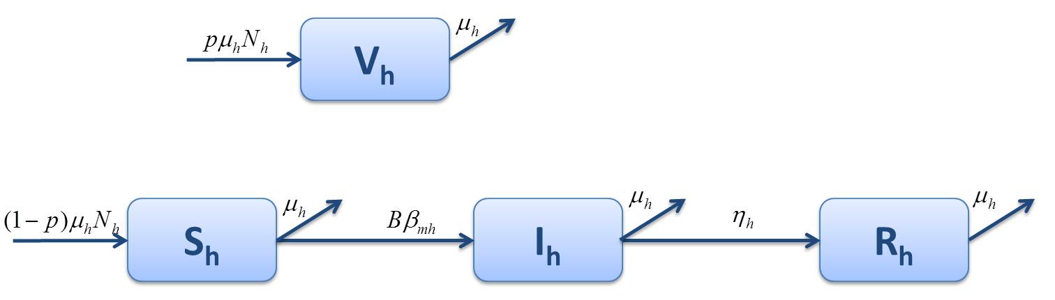
Figure 7.2: Epidemic model for human population using a pediatric vaccine

All the parameters/variables remain with the same meaning of the previous chapter. The mathematical formulation is:

$$\begin{cases}\frac{dS_{h}}{dt}=(1-p)\mu_{h}N_{h}-\left(B\beta_{mh}\frac{I_{m}}{N_{h}}+\mu_{h}\right)S_{h}\\ \frac{dV_{h}}{dt}=p\mu_{h}N_{h}-\mu_{h}V_{h}\\ \frac{dI_{h}}{dt}=B\beta_{mh}\frac{I_{m}}{N_{h}}S_{h}-(\eta_{h}+\mu_{h})I_{h}\\ \frac{dR_{h}}{dt}=\eta_{h}I_{h}-\mu_{h}R_{h}\\ \frac{dA_{m}}{dt}=\varphi\left(1-\frac{A_{m}}{kN_{h}}\right)(S_{m}+I_{m})-\left(\eta_{A}+\mu_{A}\right)A_{m}\\ \frac{dS_{m}}{dt}=\eta_{A}A_{m}-\left(B\beta_{hm}\frac{I_{h}}{N_{h}}+\mu_{m}\right)S_{m}\\ \frac{dI_{m}}{dt}=B\beta_{hm}\frac{I_{h}}{N_{h}}S_{m}-\mu_{m}I_{m}\end{cases}$$ (7.1)

We are assuming that it is a perfect vaccine, which means that it confers life-long protection.

As a first step, it is necessary to determine the basic reproduction number without vaccination ($p=0$).

Theorem 7.2.1.

The basic reproduction number, $\mathcal{R}_{0}$, associated to the differential system (7.1) without vaccination is given by

$$\mathcal{R}_{0}=\sqrt{\frac{kB^{2}\beta_{hm}\beta_{mh}\left(-\eta_{A}\mu_{m}-\mu_{A}\mu_{m}+\varphi\eta_{A}\right)}{\varphi(\eta_{h}+\mu_{h})\mu_{m}^{2}}}.$$ (7.2)

Proof.

The proof of this theorem is similar to the one in the previous chapter (see proof of Theorem 6.1.2). Just consider

$$\mathcal{F}(x)=\left(\begin{array}[]{c}B\beta_{mh}\frac{I_{m}}{N_{h}}S_{h}\\ B\beta_{hm}\frac{I_{h}}{N_{h}}S_{m}\\ \end{array}\right),\quad\mathcal{V}(x)=\left(\begin{array}[]{c}(\eta_{h}+\mu_{h})I_{h}\\ \mu_{m}I_{m}\\ \end{array}\right).$$

∎

In this chapter, we make all the simulations in two scenarios: an epidemic and an endemic situation (programming codes available in [110]). For these, the following parameter values of the differential system and initial conditions were used (Tables 7.1 and 7.2).

Parameter	Epidemic scenario	Endemic scenario
$N_{h}$	480000	480000
$B$	0.8	0.75
$\beta_{mh}$	0.375	0.21
$\beta_{hm}$	0.375	0.21
$\mu_{h}$	$\frac{1}{71\times 365}$	$\frac{1}{71\times 365}$
$\eta_{h}$	$\frac{1}{3}$	$\frac{1}{3}$
$\mu_{m}$	$\frac{1}{10}$	$\frac{1}{10}$
$\varphi$	6	6
$\mu_{A}$	$\frac{1}{4}$	$\frac{1}{4}$
$\eta_{A}$	0.08	0.08
$m$	3	3
$k$	3	3

Table 7.1: Parameters values of the differential system (7.1)

Initial conditions	Epidemic scenario	Endemic scenario
$S_{h0}$	479990	379990
$V_{h0}$	0	0
$I_{h0}$	10	10
$R_{h0}$	0	100000
$A_{m0}$	1440000	1440000
$S_{m0}$	1440000	1440000
$I_{m0}$	0	0

Table 7.2: Initial conditions of the differential system (7.1)

There were two main differences between the epidemic episode and an endemic situation. Firsty, in the endemic situation there was a slight decrease in the average daily biting $B$ and transmission probabilities $\beta_{mh}$ and $\beta_{hm}$, that could be explained by the fact that the mosquito could have more difficulties to find a naive individual. The second difference is concerned with the strong increase of the initial human population that is resistant to the disease. This may be explained by the fact that the disease, in an endemic situation, already creates an immune resistance to the infection, i.e., the population already has herd immunity. With these values we obtain approximately $\mathcal{R}_{0}=2.46$ and $\mathcal{R}_{0}=1.29$ for epidemic and endemic scenarios, respectively.

During an outbreak, the disease transmission assumes different behaviors, according to the distinct scenarios, as can been seen in Figure 7.3. In one year, the peak in an epidemic situation could reach more than 80000 cases. In contrast, instead in the endemic situation the curve of infected individuals has a more smooth behavior and reaches a peak less than 3000 cases. Figure 7.4 relates to the mosquito population. In the endemic scenario, because a substantial part of the human population is resistant to the disease, the infected mosquitoes bite a considerable percentage of resistant host, and as consequence, the disease is not transmitted.

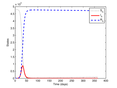
(a) Epidemic scenario

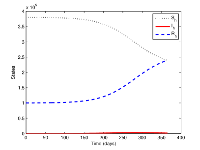
(b) Endemic scenario

Figure 7.3: Human population in a Dengue outbreak, without vaccine

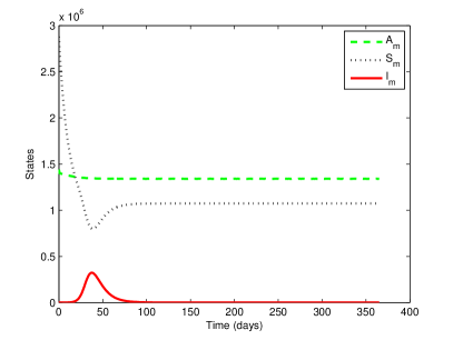
(a) Epidemic scenario

(b) Endemic scenario

Figure 7.4: Mosquito population in a Dengue outbreak, without vaccine

Suppose that at time $t=0$ a proportion $p$ of newborns are vaccinated with a perfect vaccine that causes no side effects. Since this proportion, $p$, is now immune, $\mathcal{R}_{0}$ is reduced, creating a new basic reproduction number.

Definition 19 (Basic reproduction number with pediatric vaccination).

The basic reproduction number with pediatric vaccination, $\mathcal{R}_{0}^{p}$, associated to the differential system (7.1) is given by

$$\mathcal{R}_{0}^{p}=(1-p)\mathcal{R}_{0}$$

where $\mathcal{R}_{0}$ is defined in (7.2).

Observe that $\mathcal{R}_{0}^{p}\leq\mathcal{R}_{0}$. Equality is only achieved when $p=0$, i.e., when there is no vaccination. The constraint $\mathcal{R}_{0}^{p}<1$ implicitly defines a critical vaccination portion $p>p_{c}$ that must be achieved for eradication, where

$$p_{c}=1-\frac{1}{\mathcal{R}_{0}}.$$

Since vaccination entails costs, to choose the smallest coverage that achieves eradication is the best option. This way, the entire population does not need to be vaccinated in order to eradicate the disease. This phenomenon is called herd immunity.

Vaccinating at the critical level, $p_{c}$, does not instantly lead to disease eradication. The immunity level within the population requires time to build up and at the critical level it may take a few generations before the required herd immunity is achieved. Thus, from a public health perspective, $p_{c}$ acts as a lower bound on what should be achieved, with higher levels of vaccination leading to a more rapid elimination of the disease. Figure 7.5 shows the simulations related to the proportion of newborns vaccinated ($p=0,0.25,0.50,0.75,1$) in both scenarios. Notice that at time $t=0$ no person was vaccinated. In the epidemic situation, as the outbreak reached a peak at the beginning of the year, the proportion of newborns vaccinated at that time is minimum and cannot influence the curve of infected individuals, giving the optical illusion of a single curve. On the other hand, in the endemic case, as the outbreak occurs later, the vaccination campaign starts to produce effects, decreasing the total number of sick humans. This last graphic illustrates that a vaccination campaign centered in newborns is a bet for the future of a country, but does not produce instantly results to fight the disease. To produce immediate results, it is necessary to use random mass vaccination, which means that it is necessary to vaccine a significant part of the population.

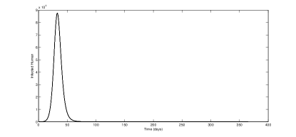
(a) Epidemic scenario

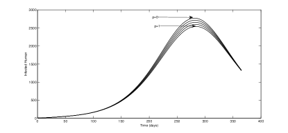
(b) Endemic scenario

Figure 7.5: Infected human in an outbreak, varying the proportion of newborns vaccinated ($p=0,0.25,0.50,0.75,1$)

7.2.2 Perfect random mass vaccination

A mass vaccination program may be initiated whenever there is an increase of the risk of an epidemic. In such situations, there is a competition between the exponential increase of the epidemic and the logistical constraints upon mass vaccination. For most human diseases it is possible, and more efficient, to not vaccinate those individuals who have recovered from the disease because they are already protected. Another situation could be the introduction of a new vaccine in a population that lives an endemic situation.

Let us consider the control technique of constant vaccination of susceptibles. In this scheme a fraction $0\leq\psi\leq 1$ of the entire susceptible population, not just newborns, is being continuously vaccinated. It is assumed that the permanent immunity acquired by vaccination is the same as natural immunity obtained from infected individuals in recovery. The epidemiological scheme is presented in Figure 7.6.

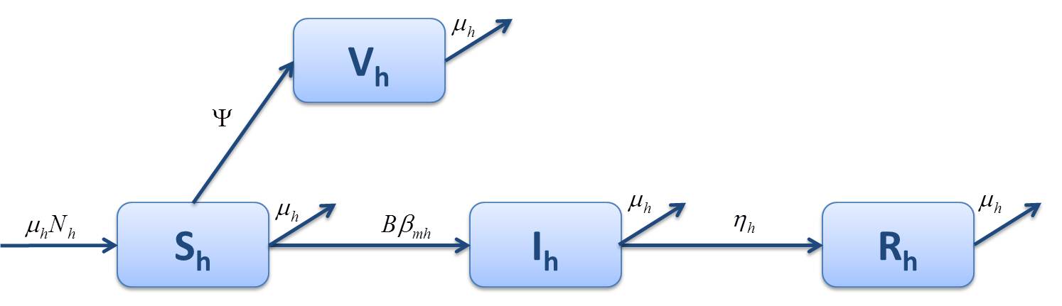
Figure 7.6: Epidemic model for human population using a mass random vaccine

The mathematical formulation for human population (the differential equations related to the mosquito remain equal to the previous subsection) is given by:

$$\begin{cases}\frac{dS_{h}}{dt}=\mu_{h}N_{h}-\left(B\beta_{mh}\frac{I_{m}}{N_{h}}+\psi+\mu_{h}\right)S_{h}\\ \frac{dV_{h}}{dt}=\psi S_{h}-\mu_{h}V_{h}\\ \frac{dI_{h}}{dt}=B\beta_{mh}\frac{I_{m}}{N_{h}}S_{h}-(\eta_{h}+\mu_{h})I_{h}\\ \frac{dR_{h}}{dt}=\eta_{h}I_{h}-\mu_{h}R_{h}\\ \end{cases}$$ (7.3)

For this model, we define a new basic reproduction number.

Definition 20 (Basic reproduction number with random mass vaccination [145]).

The basic reproduction number with random mass vaccination, $\mathcal{R}_{0}^{\psi}$, associated to the differential system (7.3) is

$$\mathcal{R}_{0}^{\psi}=\mathcal{R}_{0}\left(\frac{\mu_{h}}{\mu_{h}+\psi}\right),$$ (7.4)

where $\mathcal{R}_{0}$ is defined in (7.2).

Comparing this model with the constant vaccination of newborns model, it is apparent that instead of constantly vaccinating a portion of newborns, a part of the entire susceptible population is now being continuously vaccinated. Since the natural birth rate $\mu_{h}$ is usually small, the fraction $p\mu_{h}$ of newborns being continuously vaccinated will be small, whereas in this model, will be also a larger group of susceptibles can be continuously vaccinated, $\psi S_{h}$. Due to this, we expect that this model should require a smaller proportion of $\psi$ to achieve eradication.

Notice that $\mathcal{R}_{0}^{\psi}\leq\mathcal{R}_{0}$. Equality is only achieved in the limit $\psi=0$, that is, when there is no vaccination. The constraint $\mathcal{R}_{0}^{\psi}<1$ implicitly defines a critical vaccination portion $\psi>\psi_{c}$ that must be achieved for eradication, where

$$\psi_{c}=\left(\mathcal{R}_{0}-1\right)\mu_{h}.$$

Figure 7.7 illustrates the variation of the number of infected people when a mass vaccination is introduced. The graphs present five simulations using different proportions of the vaccinated population: $\psi=0.05,0.10,0.25,0.50,1$. Observe that in spite of the calculations done in the period of 365 days, the figures only show suitable windows, in order to provide a better analysis. In both scenarios, even with a small coverage of population, vaccination dramatically decreases the number of infected. The epidemic scenario has changed from less than 80000 cases (with no vaccination, Figure 7.3) to less than 1200 cases vaccinating only 5% of population. In the endemic scenario, the decrease is more accentuated.

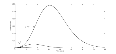
(a) Epidemic scenario

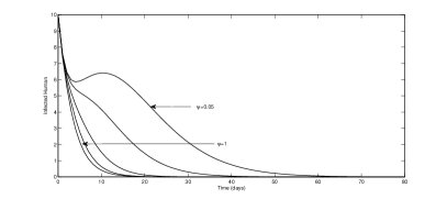
(b) Endemic scenario

Figure 7.7: Infected human in an outbreak, varying the proportion of susceptible population vaccinated ($\psi=0.05,0.10,0.25,0.50,1$)

Until here, we have considered a perfect vaccine, which means that every vaccinated individual remains resistant to the disease. However, a majority of the available vaccines for the human population does not produce 100% success in the disease battle. Usually, the vaccines are imperfect, which means that a minor percentage of cases, in spite of vaccination, are infected.

7.2.3 Imperfect random mass vaccination

Most of the theory on the disease evolution is based on the assumption that the host population is homogeneous. Individual hosts, however, may differ and they may constitute very different habitats. In particular, some habitats may provide more resources or be more vulnerable to virus exploitation [56]. The use of models with imperfect vaccines can describe better this type of human heterogeneity. Another explanation for the use of imperfect vaccines is that until now we had considered models that assumed that as soon as individuals begin the vaccination process, they become immediately immune to the disease. However, the time it takes for individuals to obtain immunity by completing a vaccination process cannot be ignored, because meanwhile an individual can be infected.

In this section a continuous vaccination strategy is considered, where a fraction $\psi$ of the susceptible class was vaccinated. The vaccination may reduce but not completely eliminate susceptibility to infection. For this reason we consider a factor $\sigma$ as the infection rate of vaccinated members. When $\sigma=0$ the vaccine is perfectly effective and when $\sigma=1$ the vaccine has no effect at all. The value $1-\sigma$ can be understood as the efficacy level of the vaccine.

The new model for the human population is represented in Figure 7.8.

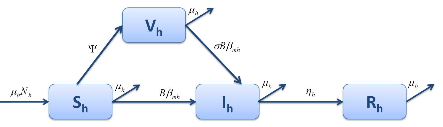
Figure 7.8: Epidemiological $SVIR$ model for human population with an imperfect vaccine

Therefore, the differential system is as follows:

$$\begin{cases}\frac{dS_{h}}{dt}=\mu_{h}N_{h}-\left(B\beta_{mh}\frac{I_{m}}{N_{h}}+\psi+\mu_{h}\right)S_{h}\\ \frac{dV_{h}}{dt}=\psi S_{h}-\left(\sigma B\beta_{mh}\frac{I_{m}}{N_{h}}+\mu_{h}\right)V_{h}\\ \frac{dI_{h}}{dt}=B\beta_{mh}\frac{I_{m}}{N_{h}}(S_{h}+\sigma V_{h})-(\eta_{h}+\mu_{h})I_{h}\\ \frac{dR_{h}}{dt}=\eta_{h}I_{h}-\mu_{h}R_{h}.\end{cases}$$ (7.5)

For this system of differential equations, we have a new basic reproduction number.

Definition 21 (Basic reproduction number with an imperfect vaccine [85]).

The basic reproduction number with an imperfect vaccine, $\mathcal{R}_{0}^{\sigma}$, associated to the differential system (7.5) is

$$\mathcal{R}_{0}^{\sigma}=\left(1+\sigma\psi\right)\frac{\mu_{h}}{\mu_{h}+\psi}\mathcal{R}_{0}=\left(1+\sigma\psi\right)\mathcal{R}_{0}^{\psi},$$

where $\mathcal{R}_{0}$ is defined in (7.2).

Notice that $\mathcal{R}_{0}^{\psi}\leq\mathcal{R}_{0}^{\sigma}$ and when the vaccine is perfect ($\sigma=0$), $\mathcal{R}_{0}^{\sigma}$ degenerates into $\mathcal{R}_{0}^{\psi}$. In other words, a high efficacy vaccine leads to a lower vaccination coverage to eradicate the disease. However, it is noted in [85] that it is much more difficult to increase the efficacy level of the vaccine when compared to controlling the vaccination rate $\psi$.

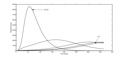
(a) Epidemic scenario

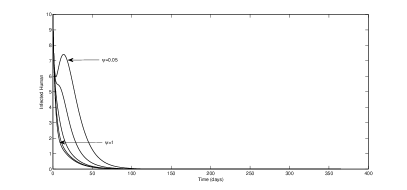
(b) Endemic scenario

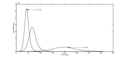
(c) Epidemic scenario

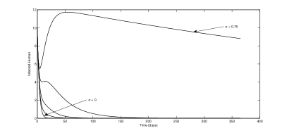
(d) Endemic scenario

Figure 7.9: Infected humans in an outbreak: in cases (a) and (b) varying the proportion of susceptible population vaccinated ($\psi=0.05,0.10,0.25,0.50,1$) with a vaccine simulating 80% of effectiveness ($\sigma=0.2$); in cases (c) and (d) varying the efficacy level of the vaccine ($\sigma=0,0.10,0.20,0.50,0.75$) and considering that 85% of the human population is vaccinated ($\psi=0.85$)

Figure 7.9 shows several simulations, by varying the vaccine efficacy and the percentage of population that is vaccinated. Comparing with Figure 7.7a, in the epidemic scenario with a perfect vaccine, the number of human infected has reached to a maximum peak of 1200 cases per day, in the worst scenario ($\psi=0.05$). Using an imperfect vaccine, with a level of efficacy of 80% (Figure 7.9a), with the same values for $\psi$, the maximum peak increases until 9000 cases.

We conclude that production of a vaccine with a high level of efficacy has a preponderant role in the reduction of the disease spread. Figures 7.9c and 7.9d reinforce the previous sentence. Assuming that 85% of the population is vaccinated, the numbers of infected cases decreases sharply with the increasing of the effectiveness level of the vaccine.

According to [34], an acceptable level of efficacy is at least 80% against all four serotypes, and 3 to 5 years for the length of protection. These are commonly considered across countries, as the minimum acceptable levels.

In the next subsection we study another type of imperfect vaccine: a vaccine that confers a limited life-long protection.

7.2.4 Random mass vaccination with waning immunity

Until the 1990s, this was an universal assumption of mathematical models of vaccination: there is no waning of vaccine-induced immunity. This assumption was routinely made because, for most of the major vaccines against childhood infectious diseases, it is approximately correct [119].

Suppose that the immunity, obtained by the vaccination process, is temporary. Assume that immunity has the waning rate $\theta$. Then the model for humans is given by

$$\begin{cases}\frac{dS_{h}}{dt}=\mu_{h}N_{h}+\theta V_{h}-\left(B\beta_{mh}\frac{I_{m}}{N_{h}}+\psi+\mu_{h}\right)S_{h}\\ \frac{dV_{h}}{dt}=\psi S_{h}-\left(\theta+\mu_{h}\right)V_{h}\\ \frac{dI_{h}}{dt}=B\beta_{mh}\frac{I_{m}}{N_{h}}S_{h}-(\eta_{h}+\mu_{h})I_{h}\\ \frac{dR_{h}}{dt}=\eta_{h}I_{h}-\mu_{h}R_{h}.\end{cases}$$ (7.6)

This model can be represented by the following epidemiological scheme (Figure 7.10).

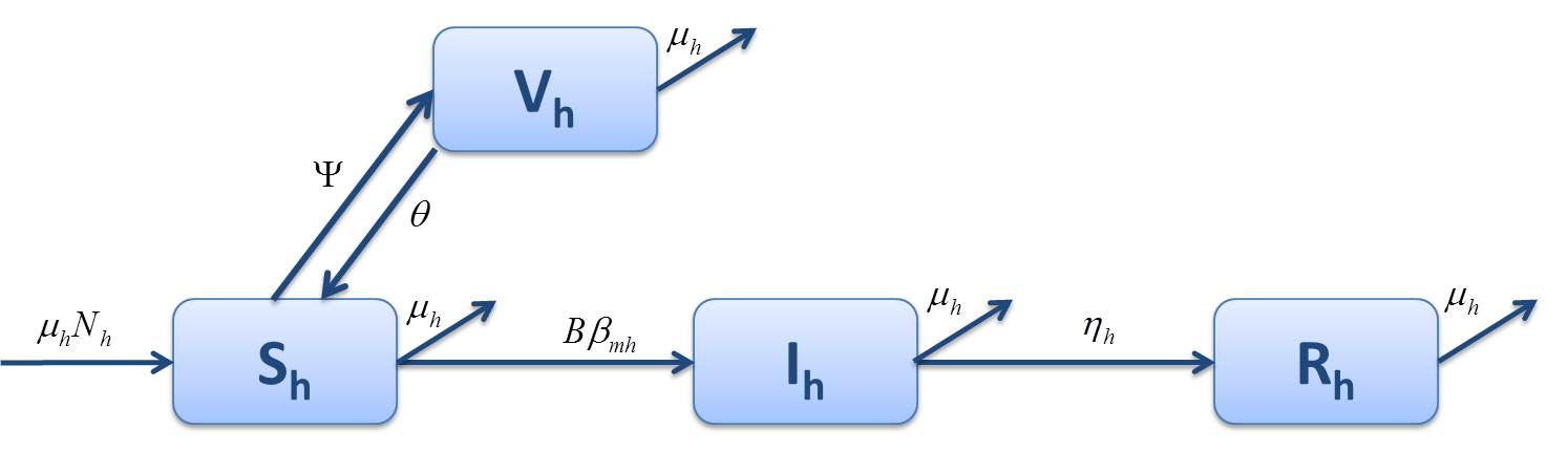
Figure 7.10: Epidemiological $SVIR$ model for human population with a waning immunity vaccine

This leads naturally to a new basic reproduction number.

Definition 22 (Basic reproduction number with an imperfect vaccine).

The basic reproduction number with an imperfect vaccine, $\mathcal{R}_{0}^{\theta}$, associated to the differential system (7.6) is

$$\mathcal{R}_{0}^{\theta}=\mathcal{R}_{0}^{\psi}$$

where $\mathcal{R}_{0}^{\psi}$ is defined in (7.4).

According to [125], the basic reproduction numbers are the same, $\mathcal{R}_{0}^{\theta}$ and $\mathcal{R}_{0}^{\psi}$, because the disease will still spread at the same rate with or without temporary immunity. However, we should expect that the convergence rate will be different between the random mass vaccination and random mass vaccination with waning immunity, since the disease will be eradicated faster in the constant treatment model without waning immunity compared to the other with waning immunity.

Figure 7.11 illustrates this statement. Considering that 85% of human population is vaccinated, the number of infected is increasing as the value of the waning immunity is growing ($\theta=0,0.05,0.10,0.15,0.20$).

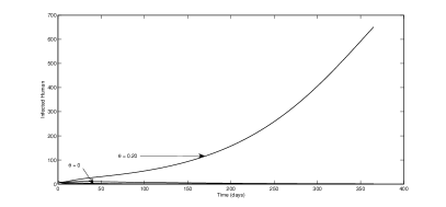
(a) Epidemic scenario

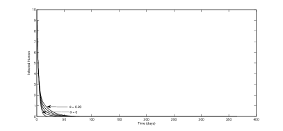
(b) Endemic scenario

Figure 7.11: Infected humans in an outbreak considering 85% of human population vaccinated ($\psi=0.85$) and varying waning immunity $(\theta=0,0.05,0.10,0.15,0.20$)

Depending on the vaccine that will be available on the market, it will be possible to choose or even combine features. In the next section we will define the vaccination process as a control system.

7.3 Vaccine as a control

In this section we consider a SIR model for humans and an ASI model for mosquitoes. The parameters remain the same as in the previous chapter.

The vaccination is seen as a control variable to reduce or even eradicate the disease. Let $u$ be the control variable related to the proportion of susceptible humans that are vaccinated. A random mass vaccination with waning immunity is selected. In this way, a parameter $\theta$ associated to the control $u$ represents the waning immunity process. Figure 7.12 shows the epidemiological scheme for the human population.

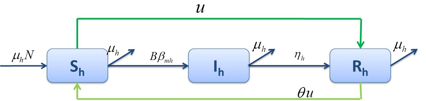
Figure 7.12: Epidemiological $SIR$ model for the human population using the vaccine as a control

The model is described by an initial value problem with a system of six differential equations:

$$\begin{cases}\frac{dS_{h}}{dt}=\mu_{h}N_{h}-\left(B\beta_{mh}\frac{I_{m}}{N_{h}}+\mu_{h}+u\right)S_{h}+\theta uR_{h}\\ \frac{dI_{h}}{dt}=B\beta_{mh}\frac{I_{m}}{N_{h}}S_{h}-(\eta_{h}+\mu_{h})I_{h}\\ \frac{dR_{h}}{dt}=\eta_{h}I_{h}+uS_{h}-\left(\theta u+\mu_{h}\right)R_{h}\\ \frac{dA_{m}}{dt}=\varphi\left(1-\frac{A_{m}}{kN_{h}}\right)(S_{m}+I_{m})-\left(\eta_{A}+\mu_{A}\right)A_{m}\\ \frac{dS_{m}}{dt}=\eta_{A}A_{m}-\left(B\beta_{hm}\frac{I_{h}}{N_{h}}+\mu_{m}\right)S_{m}\\ \frac{dI_{m}}{dt}=B\beta_{hm}\frac{I_{h}}{N_{h}}S_{m}-\mu_{m}I_{m}\end{cases}$$ (7.7)

The main aim is to study the optimal vaccination strategy, considering both the costs of treatment of infected individuals and the costs of vaccination. The objective is to

$$\text{ minimize }J[u]=\int_{0}^{t_{f}}\left[\gamma_{D}I_{h}(t)^{2}+\gamma_{V}u(t)^{2}\right]dt,$$ (7.8)

where $\gamma_{D}$ and $\gamma_{V}$ are positive constants representing the weights of the costs of treatment of infected and vaccination, respectively.

Using OC theory is possible to solve the problem.

7.3.1 Pontryagin’s Maximum Principle

Let us consider the following set of admissible control functions:

$$\Delta=\{u(\cdot)\in(L^{\infty}(0,t_{f}))|0\leq u(t)\leq 1,\forall t\in[0,t_{f}]\}.$$

Theorem 7.3.1.

Problem (7.7)-(7.8) with initial conditions in Table (7.2), admits a unique optimal solution $\left(S_{h}^{*}(\cdot),I_{h}^{*}(\cdot),R_{h}^{*}(\cdot),A_{m}^{*}(\cdot),S_{m}^{*}(\cdot),I_{m}^{*}(\cdot)\right)$ associated with an optimal control $u^{*}(\cdot)$ on $[0,t_{f}]$, with a fixed final time $t_{f}$. Moreover, there exists adjoint functions, $\lambda_{i}^{*}(\cdot)$, $i=1...6$ such that

$$\left\{\begin{array}[]{l}\dot{\lambda}_{1}^{*}=(\lambda_{1}-\lambda_{2})\left(B\beta_{mh}\frac{I_{m}}{N_{h}}\right)+\lambda_{1}\mu_{h}+(\lambda_{1}-\lambda_{3})u\\ \dot{\lambda}_{2}^{*}=-2\gamma_{D}I_{h}+\lambda_{2}(\eta_{h}+\mu_{h})-\lambda_{3}\eta_{h}+(\lambda_{5}-\lambda_{6})\left(B\beta_{hm}\frac{S_{m}}{N_{h}}\right)\\ \dot{\lambda}_{3}^{*}=-\lambda_{1}\theta u+\lambda_{3}(\mu_{h}+\theta u)\\ \dot{\lambda}_{4}^{*}=\lambda_{4}\varphi\frac{S_{m}+I_{m}}{kN_{h}}+\lambda_{4}(\eta_{A}+\mu_{A})-\lambda_{5}\eta_{A}\\ \dot{\lambda}_{5}^{*}=-\lambda_{4}\varphi\left(1-\frac{A_{m}}{kN_{h}}\right)+(\lambda_{5}-\lambda_{6})B\beta_{hm}\frac{I_{h}}{N_{h}}+\lambda_{5}\mu_{m}\\ \dot{\lambda}_{6}^{*}=(\lambda_{1}-\lambda_{2})\left(B\beta_{mh}\frac{S_{h}}{N_{h}}\right)-\lambda_{4}\varphi\left(1-\frac{A_{m}}{kN_{h}}\right)+\lambda_{6}\mu_{m}\\ \end{array}\right.$$

(7.9)

with the transversality conditions $\dot{\lambda}_{i}(t_{f})=0$, i=1, …6. Furthermore,

$$u^{*}=\min\left\{1,\max\left\{0,\frac{\left(\lambda_{1}-\lambda_{3}\right)\left(S_{h}-\theta R_{h}\right)}{2\gamma_{V}}\right\}\right\}.$$ (7.10)

Proof.

The existence of optimal solutions $\left(S_{h}^{*}(\cdot),I_{h}^{*}(\cdot),R_{h}^{*}(\cdot),A_{m}^{*}(\cdot),S_{m}^{*}(\cdot),I_{m}^{*}(\cdot)\right)$ associated to the optimal control $u^{*}(\cdot)$ comes from the convexity of the integrand of the cost function (7.8) with respect to the control $u$ and the Lipschitz property of the state system with respect to state variables $\left(S_{h},I_{h},R_{h},A_{m},S_{m},I_{m}\right)$ (for more details see [24]). According to the Pontryagin Maximum Principle [106], if $u^{*}(\cdot)\in\Delta$ is optimal for the problem considered, then there exists a nontrivial absolutely continuous mapping $\lambda:[0,t_{f}]\rightarrow\mathbb{R}$, $\lambda(t)=\left(\lambda_{1}(t),\lambda_{2}(t),\lambda_{3}(t),\lambda_{4}(t),\lambda_{5}(t),\lambda_{6}(t)\right)$, called the adjoint vector, such that

$$\begin{cases}\dot{S}_{h}=\frac{\partial H}{\partial\lambda_{1}}\\ \dot{I}_{h}=\frac{\partial H}{\partial\lambda_{2}}\\ \dot{R}_{h}=\frac{\partial H}{\partial\lambda_{3}}\\ \dot{A}_{m}=\frac{\partial H}{\partial\lambda_{4}}\\ \dot{S}_{m}=\frac{\partial H}{\partial\lambda_{5}}\\ \dot{I}_{m}=\frac{\partial H}{\partial\lambda_{6}}\\ \end{cases}$$ (7.11)

and

$$\begin{cases}\dot{\lambda}_{1}=-\frac{\partial H}{\partial S_{h}}\\ \dot{\lambda}_{2}=-\frac{\partial H}{\partial I_{h}}\\ \dot{\lambda}_{3}=-\frac{\partial H}{\partial R_{h}}\\ \dot{\lambda}_{4}=-\frac{\partial H}{\partial A_{m}}\\ \dot{\lambda}_{5}=-\frac{\partial H}{\partial S_{m}}\\ \dot{\lambda}_{6}=-\frac{\partial H}{\partial I_{m}}\\ \end{cases}$$ (7.12)

where the Hamiltonian $H$ is defined by

$$H$$

and the minimality condition

$$H\left(S_{h}^{*}(t),I_{h}^{*}(t),R_{h}^{*}(t),A_{m}^{*}(t),S_{m}^{*}(t),I_{m}^{*}(t),\lambda^{*}(t),u^{*}(t)\right)$$

(7.13)

holds almost everywhere on $[0,t_{f}]$. Moreover, the transversality conditions $\lambda_{i}(t_{f})=0$, $i=1,\ldots 6,$ hold. System (7.9) is derived from (7.12), and the optimal control (7.10) comes from the minimality condition (7.13). ∎

7.3.2 Numerical simulation and discussion

The simulations were carried out using the values of the previous section. The system was normalized, using the same strategy as in Chapter 5. It was considered that the waning immunity was at a rate of $\theta=0.05$. The OC problem was solved using two methods: direct [9, 133] and indirect [81]. The direct method uses the cost functional (7.8) and the state system (7.7) and was solved by DOTcvp [67]. The indirect method used is an iterative method with a Runge–Kutta scheme, solved through ode45 of MatLab.

Figure 7.13 shows the optimal control obtained by both methods. Notice that DOTcvp only gives the optimal control as a constant piecewise function. Table 7.3 shows the costs obtained by the two methods in both scenarios. The indirect method gives a lower cost. This method uses more mathematical theory about the problem, such as the adjoint system (7.11) and optimal control expression (7.10). Therefore it makes sense that the indirect method produces a better solution.

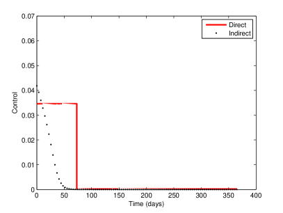
(a) Epidemic scenario

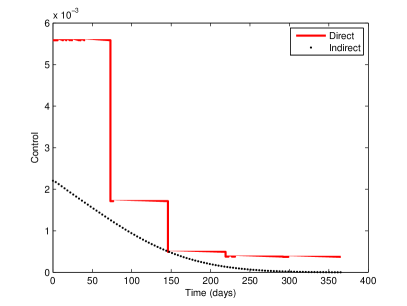
(b) Endemic scenario

Figure 7.13: Optimal control with direct and indirect approach in both scenarios

Method	Epidemic scenario	Endemic scenario
Direct (DOTcvp)	0.07505791	0.00189056
Indirect (backward-forward)	0.06070556	0.00080618

Table 7.3: Optimal values of the cost functional (7.8)

Using the optimal solution as reference, some tests were performed, regarding infected individuals and costs, when no control ($u\equiv 0$) or upper control ($u\equiv 1$) is applied.

Table 7.4 shows the results for DOTcvp in the three situations. In both scenarios, using the optimal strategy of vaccination produces better costs with the disease, when compared to not doing anything. Once there is no control, the number of infected humans is higher and produces a more expensive cost functional.

	Epidemic scenario	Endemic scenario
optimal control	0.07505791	0.00189056
no control	0.32326592	0.01045990
upper control	147.82500296	116.800000275

Table 7.4: Values of the cost functional with optimal control, no control ($u\equiv 0$) and upper control ($u\equiv 1$)

Figure 7.14 shows the number of infected humans when different controls are considered. It is possible to see that using the upper control, which means that everyone is vaccinated, implies that just a few individuals were infected, allowing eradication of the disease. Although the optimal control, in the sense of objective (7.8), allows the occurrence of an outbreak, the number of infected individuals is much lower when compared with a situation where no one is vaccinated.

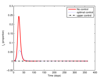
(a) Epidemic scenario

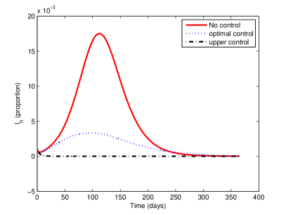
(b) Endemic scenario

Figure 7.14: Optimal control obtained from a direct and indirect approach in both scenarios

We conclude that a vaccination campaign in the susceptible population, and assuming a considerable efficacy level of the vaccine, can quickly decrease the number of infected people.

7.4 Conclusions

The worldwide expansion of the Dengue fever is a growing health problem. Dengue vaccine is an urgent challenge that needs to be overcome. This may be commercially available within a few years, when the researchers find a formula that protect against all four Dengue viruses. A vaccination program is seen as an important measure used in infectious disease control and immunization and eradication programs.

In the first part of the chapter, different types of vaccine, as well as their features and some of coverage thresholds, were introduced. The main idea was to study some types of vaccines in order to cover most of the future vaccine features. The main goal of a vaccination program is to reduce the prevalence of an infectious disease and ultimately to eradicate it. It was shown that eradication success depends on the type of vaccine as well as on the vaccination coverage. The imperfect vaccines may not completely prevent infection but could reduce the probability of being infected, thereby reducing the disease burden. In this study all the simulations were done using epidemic and endemic scenarios to illustrate distinct realities.

A second analysis was made, using an OC approach. The vaccine behaved as a new disease control variable and, when available, can be a promising strategy to fight the disease.

Dengue is an infectious tropical disease difficult to prevent and manage. Researchers agree that the development of a vaccine for Dengue is a question of high priority. In the present study we have shown how a vaccine results in saving lives and at the same time in a reduction of the budget related with the disease. As future work we intend to study the interaction of a Dengue vaccine with other kinds of control already investigated in the literature, such as insecticide and educational campaigns [113, 118].

This chapter was based on work accepted in the peer reviewed proceedings [114].

Conclusions and future perspectives

Mathematical models can be a powerful tool to understand epidemiological phenomena. These models can be used to compare, plan, implement and evaluate several programs related to detection, prevention and control of infectious diseases. Indeed, one of the most important issues in epidemiology is to improve control strategies with the final goal to reduce or even eradicate the disease. In this thesis were constructed and analyzed some models for the spreading of diseases, particularly for Dengue Fever.

The links between health and sustainable development are illustrated for this disease. Any attempt in predicting and preventing the disasters caused by the disease will imply a global strategy that takes into account environmental conditions, levels of poverty and illiteracy and, eventually, degree of coverage by vaccination programs [35].

Although vector control strategies were already available before the Second World War, Dengue pandemic was underestimated. It became a global public health problem in the past 60 years and a major concern for WHO.

The main contributions of this thesis can be classified into three main categories, namely, model formulation, mathematical and computational analysis, and contributions to public health/intervention design.

Model formulation

Deterministic models for assessing the combined impact of several control measures in Dengue disease were considered.

In Chapter 4 an old OC problem for Dengue was revisited. It was shown that new and robust tools bring refreshing solutions to the problem. Some analysis with discretization schemes were carried out in order to understand the best way to implement the direct methods in future approaches. For this problem, is was better to use robust solvers than to implement higher order discretization methods, due to the increasing of problem’s dimension.

In Chapter 5, a SEIR+ASEI model was studied. Threshold criteria was established ensuring the disease eradication and hence convergence to the so-called disease free solution. Using real data from Cape Verde, the application of insecticide in the country during the outbreak was simulated and its repercussions were analyzed. The study of this outbreak was performed in several phases: firstly, using a previously calculated constant control for the whole period, with the aim of having a basic reproduction number below unity; then, several periodic strategies were studied in order to find the best logistics approaches to implement that keep $\mathcal{R}_{0}$ less than one; finally, an OC approach to compare with the previous suboptimal approaches was used. For this final phase, several perspectives of the problem were analyzed, including bioeconomic, medical and economic approaches. Depending of the main target to achieve, the results for the control and infected individuals vary.

In Chapter 6, a SIR+ASI model for Dengue was presented. The lost of two differential equations, was compensated by the introduction of two more controls: in addition to adulticide, larvicide and mechanical control were introduced. Similarly to Chapter 5, a threshold criteria for the eradication of the disease was established. The influence of the controls in this threshold was analyzed. Then, varying the controls, separately and simultaneously, an analysis of the importance/consequence of each control in the development of the disease was made. Finally, an OC approach using different weights for the variables in the functional was studied, in order to establish the best optimal curve for each control and the respective effects in the development/erradication of the disease.

In Chapter 7, some simulations with different types of vaccines were made. As a Dengue vaccine is not yet available, distinct hypothetical models to introduce the vaccine were studied. In Section 7.2, was considered a new compartment $V_{h}$ producing a new model SVIR+ASI. This research comprised SVIR models with perfect vaccines — constant vaccination of newborns and constant vaccination of susceptibles — and imperfect vaccines — using a level of efficacy below 100% and also with waning immunity. In Section  7.3, the vaccination process was studied as a control of the epidemic model. For this, as in the previous chapter, an OC approach was presented. All the simulations were done in epidemic and endemic scenarios, in order to understand what type of repercussions could bring each kind of vaccines.

Mathematical and computational analysis

In this work, there was a concern in producing a mathematical analysis for all new models presented. Epidemiological concepts, such as the basic reproduction number and equilibrium points, were calculated. The equilibrium points were classified and their local stability analyzed. The OC theory was used in order to provide the best strategies for each model, involving direct and indirect approaches.

Throughout the thesis, a set of software packages were used, showing the importance of the these tools in the development of some mathematical fields. To solve ODE systems, codes in Matlab and Scilab were implemented. To calculate the equilibrium points and the basic reproduction number, Mathematica and Maple were used. For the OC approach, several packages were also selected: from programmed codes in AMPL and run in NEOS Server (Ipopt, Snopt, Knitro, Muscod-II) to Fortran codes in the Linux environment (OC-ODE) or even programs coded in Matlab (DOTcvp and indirect methods). The software choice was varying during the research process, due to availability, robustness and solving speed. The main codes developed in this thesis are available at: https://sites.google.com/site/hsofiarodrigues/home/phd-codes-1 [110]. Using direct and indirect methods, the solutions obtained were similar, reinforcing the confidence in the results.

Public health/intervention design

The study provides some important epidemiological insights into the impact of vector control measures. Dengue burden decreases with the increasing of vector control measures (adulticide, larvicide and mechanical control). Furthermore, the adulticide should be the first/main measure to apply when an outbreak occurs, whereas the other two measures should be considered as a long time prevention.

The last control measure to be studied was the vaccination. It was shown that the vaccine, when available, could bring advantages not only in the reduction of infected individuals, but also decreasing the disease costs.

A PhD thesis is always an unfinished process, but some day it is necessary to stop. Therefore, some topics were not explored and can be understood as future directions of the work.

A first suggestion is to use heterogeneity for both populations, dividing each one in more compartments [84]. Human population is not immunologically homogeneous, presenting groups with distinct level of risk, related with age, sex or the presence of a disease or immunosuppressive drugs which would be the case with transplant patients or cancer suffers. For example, the transmission probability in young children is higher and generally with more severe symptoms when compared to adult transmission. Moreover, the mosquito population does not have the same behavior during the whole year, depending specially on weather conditions. Temperature and humidity are key variables on vector population dynamics. It will be interesting to add some seasonality factors into the last models [45, 101].

Another open question is the introduction of immigration and tourism issues. Along the work it was considered a constant population, but the addition of new individuals could induce new outbreaks.

Other aspect is related to the disease development in the presence of several serotypes. While in Cape Verde only one serotype was found, the interaction of several serotypes in Asia is already a reality. This will induce changes in the model, not only increasing of the number of variables but also causing a more expressive number of DHF cases [105].

Currently, Portuguese researchers are developing a new repellent for mosquito that could be considered as a new control for the disease. This product does not kill the mosquito, but prevents the bite by deviating it from the target and consequently decreasing the chain of the disease transmission.

With the viability of the vaccine, it will be possible to fit a better model according to the vaccine used. One of the possibilities is using pulse vaccination, where children at a certain age cohorts are periodically immunized [41]. The theoretical challenge of pulse vaccination is the a priori determination of the pulse interval for specific values of $\mathcal{R}_{0}$, the proportion of vaccinated $p$ and the population birth rate $\mu$.

Most of the analysis and models presented in this thesis can be adapted for other vector-borne diseases — such as malaria, yellow fever, West Nile virus, chikungunya, Japanese encephalitis — by just fitting some variables/parameters and some initial assumptions intrinsic to the disease [18, 46, 72].

When attempting to model epidemics and control for public health applications, there is the compelling urge to make models as sophisticated as possible, including many details about the host and the vector. Although this strategy may be useful when such details are known or exist suitable data, it may lead to a false sense of accuracy when reliable information is not available. Another approach is to keep the model simple and, instead of using the conventional differential calculus, to apply fractional calculus to fit to the disease reality [107] or to use the general theory of time scales [15].

“If people do not believe that mathematics is simple, it is only because they do not realize how complicated life is.”

— John Louis von Neumann, 1947

Index

• AMPL §2.3.1, §2.3.2, §2.3.2, §4.2.2, §4.3, Part II
• Basic reproduction number Figure 3.6, §3.2, §3.3, §3.4.1, §3.4.2, §3.5, §3.6, §5.1.1, §5.1.1, §5.1.2, §5.2, §6.1, §6.1, Theorem 6.1.2, Theorem 7.2.1, Introduction, Part II, Part II, Definition 17, Definition 19, Definition 20, Definition 21, Definition 22, Definition 8, Remark 7
• Bolza form Theorem 1.2.1, Definition 2
• Direct method §2.2, §2.3, §2.3, §2.3, §2.3.2, §4.4, §5.3.2, §5.3.2, §7.3.2, Introduction, Part II
• Disease Free Equilibrium §3.4.2, §3.5, §3.6, §3.7, §3.7, 1st item, §5.1.1, §5.1.1, §5.1.1, §5.1.1, §5.1.1, §5.1.2, Theorem 5.1.1, §5.2, §5.2, §5.4, §6.1, Theorem 6.1.1, Theorem 6.1.1, Introduction, Definition 14, Definition 18, Example 11, Example 12
• DOTcvp §2.3.1, §5.3.2, §5.3.2, §5.3.2, §5.3.2, §6.3, §7.3.2, §7.3.2, Part II
• Endemic Equilibrium §3.4.2, §3.4.2, §3.5, §3.6, Theorem 5.1.3, §5.4, Theorem 6.1.1, Theorem 6.1.1, Theorem 6.1.3, Definition 14, Definition 18, Example 11
• Equilibrium point §3.4.2, §3.5, §5.1.1, §5.1.1, §6.1, Introduction, Part II, Definition 14, Definition 18
• Euler scheme §2.1, §4.2.2, §4.3, §4.3
• Hamiltonian §1.3, §2.2, §5.3.1, §5.3.1, §7.3.1, Definition 4, Example 4, Proposition 3, Remark 2
• Herd immunity §4.1.2, §5.1.2, §6.4, Chapter 7, §7.2.1, §7.2.1
• Indirect methods §2.2, §2.2, §5.3.2, §5.3.2, §7.3.2, §7.3.2, Introduction, Part II
• Ipopt §2.3.1, §2.3.2, §4.2.2, §4.2.2, §4.2.2, §4.2.2, §4.3, §4.4, §5.3.2, Part II
• Knitro §2.3.2, §4.3, §4.3, Part II
• Lagrange form §1.2, Theorem 1.2.1, §4.2.1, Definition 1
• Maple §6.1, §6.1, Part II
• Mathematica §5.1.1, §5.1.1, §5.1.1, §5.1.2, Part II
• Matlab §2.2, §2.3.1, §5.3.2, §5.3.2, §6.2, §7.3.2, Part II
• Mayer form §1.2, Theorem 1.2.1, §2.3.1, §4.2.1, §5.3.2, Definition 3
• Multiple shooting method §2.1, §2.1, §2.1, §4.2.2
• Muscod-II §2.3.1
• NEOS platform §2.3.1, §2.3.2, §2.3.2, §4.3, §4.3, Part II
• OC-ODE §2.3.1, §4.2.2, §4.2.2, §4.2.2, §4.4, §5.3.2, §5.3.2, Part II
• ode45 routine §2.2, §5.3.2, §6.2, §7.3.2
• Optimality condition Proposition 1, §1.3, §1.5, §2.2, §2.2, Proposition 2, Proposition 3, Remark 4
• Pontryagin’s Maximum Principle §1.3, Theorem 1.3.1, §1.4, §2.2, §5.3.1, §7.3.1, Introduction, Proposition 2
• Runge Kutta scheme §2.1, §4.3, §4.3, §6.2, §7.3.2
• Scilab §5.1.2, §6.3, Part II, Part II
• Shooting method §2.1, §2.1
• Snopt §2.3.2, §4.3, §4.3, Part II
• Transversality condition Proposition 1, Proposition 2, §2.2, §2.2, §5.3.1, §5.3.1, §7.3.1, Theorem 7.3.1, Example 1, Example 4, Proposition 3, Proposition 3, Remark 1

References

- [1] A. Abate, A. Tiwari, and S. Sastry. Box invariance in biologically-inspired dynamical systems. Automatica, 45(7):1601–1610, 2009.
- [2] África21. Mosquito transmissor da dengue chega a Cabo Verde. http://www.africa21digital.com/noticia.kmf?cod=7617981&canal=404, Jan 2012.
- [3] L. J. Allen and P. v. d. Driessche. The basic reproduction number in some discrete-time epidemic models. J. Difference Equ. Appl., 14(10-11):1127–1147, 2008.
- [4] E. S. Allman and J. A. Rhodes. Mathematical Models in Biology: an introduction. Cambridge University Press, 2004.
- [5] M. J. Alves, H. Osório, and L. Zé-Zé. Relatório REVIVE 2011 - culicídeos. Technical report, Instituto Nacional de Saúde Doutor Ricardo Jorge, 2011.
- [6] R. M. Anderson and R. M. May. Infectious Diseases of Humans. Oxford University Press, 1991.
- [7] R. M. Anderson and R. M. May. Directly transmitted infectious diseases: control by vaccination. Science, 215:1053–1060, 2005.
- [8] A. C. Bartlett and R. T. Staten. Radcliffe’s IPM World Textbook, chapter The sterile release method and other genetic control atrategies. University of Minesota, 1996. http://ipmworld.umn.edu.
- [9] J. Betts. Practical Methods for Optimal Control Using Nonlinear Programming. SIAM: Advances in Design and Control, 2001.
- [10] J. E. Blaney, N. S. Sathe, C. T. Hanson, C. Y. Firestone, B. R. Murphy, and S. S. Whitehead. Vaccine candidates for dengue virus type 1 (den1) generated by replacement of the strutural genes of rden4 and rden430 with those of den1. Virology Journal, 4(23):1–11, 2007.
- [11] S. M. Blower, P. M. Small, and P. C. Hopewell. Control strategies for tuberculosis epidemics: New models for old problems. Science, 273(5274):497–500, 1996.
- [12] B. Bonnard and G. Janin. Geometric orbital transfer using averaging techniques. J. Dyn. Control Syst., 14(2):145–167, 2008.
- [13] I. A. Braga and D. Valle. Aedes aegypti: insecticidas, mecanismos de ação e resistência. Epidemiol. Serv. Saúde, Brasília, 16(4):279–293, 2007.
- [14] F. Brauer. Compartmental models in epidemiology. In Mathematical epidemiology, volume 1945 of Lecture Notes in Math., pages 19–79, Springer, Berlin, 2008.
- [15] A. M. C. Brito da Cruz, H. S. Rodrigues, and D. F. M. Torres. Escalas Temporais e Mathematica. Boletim da Sociedade Portuguesa de Matemática, 62:1–18, 2010. arXiv:0911.3187
- [16] A. E. Bryson Jr. Optimal control 1950 to 1985. IEEE Control Systems Magazine, pages 26–33, 1996.
- [17] B. Buonomo. On the optimal vaccination strategies for horizontally and vertically transmitted infectious diseases. Journal of Biological Systems, 19(2):263–279, 2011.
- [18] S. Butler, D. Kirschner, and S. Lenhart. Advances in mathematical population dynamics - molecules, cells and man, volume 6 of Ser. Math. Biol. Med, chapter Optimal control of chemotherapy affecting the infectivity of HIV, pages 557–569. Singapore: World Scientific Publishing, 1997.
- [19] R. H. Byrd, J. Nocedal, and R. A. Waltzy. Large-Scale Nonlinear Optimization, chapter Knitro: An Integrated Package for Nonlinear Optimization, pages 35–59. Springer-Verlag, 2006.
- [20] M. A. L. Caetano and T. Yoneyama. Optimal and sub-optimal control in dengue epidemics. Optimal Control Applications and Methods, 22:63–73, 2001.
- [21] S. L. Campbell, J. P. Chancelier, and R. Nikoukhah. Modeling and simulation in Scilab/Scicos. Springer, New York, 2006.
- [22] C. Castillo-Chavez, Z. Feng, and W. Huang. Mathematical Approaches for Emerging and Reemerging Infectious Diseases: An Introduction, volume 125, Chapter on the computation of and its role in global stability, pages 229–250. Springer, 2002.
- [23] P. Cattand and et al. Disease Control Priorities in Developing Countries, chapter Tropical Diseases Lacking Adequate Control Measures: Dengue, Leishmaniasis, and African Trypanosomiasis, pages 451–466. DCPP Publications, 2006.
- [24] L. Cesari. Optimization—theory and applications. Problems with ordinary differential equations. Applications of Mathematics, 17. New York - Heidelberg - Berlin: Springer-Verlag, 1983.
- [25] B. Chachuat. Nonlinear and Dynamic Optimization: From Theory to Practice. Automatic Control Laboratory, EPFL, Switzerland, 2007.
- [26] G. Chowell, P. Diaz-Duenas, J. C. Miller, A. Alcazar-Velazco, P. W. Fenimore, and C. C. Chavez. Estimation of the reproduction number of dengue fever from spatial epidemic data. Mathematical Biosciences, 208(2):571–589, 2007.
- [27] S. R. Christophers. Aedes aegypti, the Yellow fever Mosquito: Its Life History, Bionomics and Structure. Cambridge University Press, London, 1960.
- [28] D. V. Clark and et al. Economic impact of dengue fever / dengue hemorrhagic fever in Thailand at the family and population levels. Am J Trop Med Hyg, 72(6):786–791, 2005.
- [29] F. H. Clarke. Optimization and nonsmooth analysis, volume 5 of Classics in Applied Mathematics. Society for Industrial and Applied Mathematics (SIAM), Philadelphia, PA, second edition, 1990.
- [30] G. Coelho, M. Burattini, M. G. Teixeira, F. A. B. Coutinho, and E. Massad. Dynamics of the 2006/2007 dengue outbreak in brazil. Mem Inst Oswaldo Cruz, 103(6):535–539, 2008.
- [31] M. da Saúde de Cabo Verde. Dengue. http://www.minsaude.gov.cv, Jan 2012.
- [32] I. N. de Estatística de Cabo Verde. http://www.ine.cv, Sept 2011.
- [33] Dengue Virus Net. http://denguevirusnet.com, Jan 2012.
- [34] D. DeRoeck, J. Deen, and J. D. Clemens. Policymakers’ views on dengue fever/dengue haemorrhagic fever and the need for dengue vaccines in four southeast Asian countries. Vaccine, 22:121–129, 2003.
- [35] M. Derouich and A. Boutayeb. Dengue fever: Mathematical modelling and computer simulation. Appl. Math. Comput., 177(2):528–544, 2006.
- [36] M. Derouich, A. Boutayeb, and E. Twizell. A model of dengue fever. Biomedical Engineering Online, 2(4):1–10, 2003.
- [37] G. J. Devine, E. Z. Perea, G. F. Killen, J. D. Stancil, S. J. Clark, and A. C. Morrison. Using adult mosquitoes to transfer insecticides to aedes aegypti larval habitats. In Proceeding of the National Academy of Sciences of the United States of America, 2009.
- [38] O. Diekmann and J. A. P. Heesterbeek. Mathematical epidemiology of infectious diseases: model building, analysis and interpretation. New York Wiley, 2000.
- [39] O. Diekmann, J. A. P. Heesterbeek, and J. A. J. Metz. On the definition and the computation of the basic reproduction ratio in models for infectious diseases. J. Math. Biol., 35:503–522, 1990.
- [40] G. do Primeiro Ministro. Núcleo operacional da sociedade de informação. http://www.dengue.gov.cv, Jan 2012.
- [41] A. d’Onofrio. Stability properties of pulse vaccination strategy in SEIR epidemic model. Mathematical Biosciences, 179:57 –72, 2002.
- [42] P. v. d. Driessche and J. Watmough. Reproduction numbers and sub-threshold endemic equilibria for compartmental models of disease transmission. Math. Biosci., 180:29–48, 2002.
- [43] Y. Dumont and F. Chiroleu. Vector control for the chikungunya disease. Mathematical Bioscience and Engineering, 7(2):313–345, 2010.
- [44] Y. Dumont, F. Chiroleu, and C. Domerg. On a temporal model for the chikungunya disease: modeling, theory and numerics. Math. Biosci., 213(1):80–91, 2008.
- [45] J. E. Duque and M. A. Navarro-Silva. Dynamics of the control of aedes (stegomyia) aegypti linnaeus (diptera, culicidae) by bacillus thuringiensis var israelensis, related with temperature, density and concentration of insecticide. Rev. Bras. Entomol., 50(4):528–533, 2006.
- [46] A. El-Gohary and I. A. Alwasel. The chaos and optimal control of cancer model with complete unknown parameters. Chaos, Solitons & Fractals, 42(5):2865–2874, 2009.
- [47] L. Esteva and H. M. Yang. Mathematical model to assess the control of aedes aegypti mosquitoes by the sterile insect technique. Mathematical Biosciences, 198:132–147, 2005.
- [48] C. Farrington. On vaccine efficacy and reproduction numbers. Math. Biosci., 185(1):89–109, 2003.
- [49] Z. Feng and J. X. Velasco-Hernández. Competitie exclusion in a vector-host model for the dengue fever. Journal of Mathematical Biology, 35(5):523–544, 1997.
- [50] N. M. Ferguson, D. A. T. Cummings, C. Fraser, J. C. Cajka, P. C. Cooley, and D. S. Burke. Strategies for mitigating an influenza pandemic. Nature, 442:448–452, 2006.
- [51] E. M. G. P. Fernandes. Computação Numérica. Universidade do Minho, Braga, 1998.
- [52] A. F. Filippov. On certain questions in the theory of Optimal Control. SIAM Journal on Control, 1:76–84, 1968.
- [53] W. H. Fleming and R. W. Rishel. Deterministic and Stochastic Optimal Control. Springer-Verlag, 1975.
- [54] C. for Disease Control, D. o. V. B. Prevention (CDC), and I. Diseases. Prevention: How to reduce your risk of dengue infection. Technical report, Centers for Disease Control and Prevention (CDC), 2010. Available at http://www.cdc.gov/Dengue/prevention/index.html.
- [55] R. Fourer, D. M. Gay, and B. W. Kernighan. AMPL: A Modeling Language for Mathematical Programming. Duxbury Press / Brooks/Cole Publishing Company, 2002.
- [56] S. Gandon, M. Mackinnon, S. Nee, and A. Read. Imperfect vaccination: some epidemiological and evolutionary consequences. In Proceedings of Biological Sciences, volume 270, pages 1129–1136, 2003.
- [57] M. Gerdts. User’s guide OC-ODE (version 1.4). Technical report, Universität Würzburg, May 2009.
- [58] P. E. Gill and M. A. Murray, W. Sauders. Snopt: An SQP algorithm for large-scale constrained optimization. SIAM, 47(1):99–131, 2005.
- [59] B. S. Goh. Optimal singular rocket and aircraft trajectories. In Control and Decision Conference, 2008. CCDC 2008. Chinese, pages 1531–1536, July 2008.
- [60] B. Guy, J. Almond, and J. Lang. Dengue vaccine prospects: a step forward. The Lancet, 377(9763):381–382, 2011.
- [61] J. R. Heffernan, R. J. Smith, and L. M. Wahl. Perspective on the basic reproductive ratio. J. R. Soc. Interface, 2:281–293, 2005.
- [62] A. Hermant. Optimal control of the atmospheric reentry of a space shuttle by an homotopy method. Optimal Control Applications and Methods, 32(6):627–646, 2010.
- [63] H. W. Hethcote. A thousand and one epidemic models. Frontiers in Theoretical Biology, 100(504–515), 1994.
- [64] H. W. Hethcote. The mathematics of infectious diseases. SIAM Rev., 42(4), 2000.
- [65] H. W. Hethcote. Mathematical Understanding of Infectous Disease Dynamics, chapter The basic epidemiology models: models, expressions for , parameter estimation, and applications, pages 1–61. Lecture Notes Series Institute for Mathematical Sciences. National University of Singapore, 2008.
- [66] A. C. Hindmarsh and et al. Sundials: Suite of nonlinear and differential/algebraic equation solvers. ACM Transactions on Mathematical Software, 31(3):363–396, 2005.
- [67] T. Hirmajer, E. Balsa-Canto, and J. R. Banga. Dotcvpsb, a software toolbox for dynamic optimization in systems biology. Bioinformatics, 10:199–213, 2009.
- [68] J. Hombach, M. J. Cardosa, A. Sabchareon, D. W. Vaughn, and A. D. Barrett. Scientific consultation on immunological correlates of protection induced by dengue vaccines: report from a meeting held at the world health organization 17-18 november 2005. Vaccine, 25(21):4130–4139, 2007.
- [69] M. J. Hopp and J. A. Foley. Global-scale relationships between climate and the dengue fever vector, Aedes Aegypti. Climatic Change, 48:441–463, 2001.
- [70] D. Houcque. Applications of MATLAB: Ordinary differential equations (ODE). Technical report, Robert R. McCormick School of Engineering and Applied Science - Northwestern University, Evanston.
- [71] K. E. Jones, N. G. Patel, M. A. Levy, A. Storeygard, D. Balk, and J. L. Gittleman. Global trends in emerging infectious diseases. Nature, 451:990–993, 2008.
- [72] H. R. Joshi. Optimal control of an HIV immunology model. Optimal Control Appl. Methods, 23(4):199–213, 2002.
- [73] H. R. Joshi, S. Lenhart, M. Y. Li, and L. Wang. Optimal control methods applied to disease models. In Mathematical studies on human disease dynamics, volume 410 of Contemp. Math., pages 187–207. Amer. Math. Soc., Providence, RI, 2006.
- [74] J. C. Kamgang and G. Sallet. Computation of threshold conditions for epidemiological models and global stability of the disease-free equilibrium (DFE). Mathematical Biosciences, 213:1–12, 2008.
- [75] M. I. Kamien and N. L. Schwartz. Dynamic Optimization: the Calulus of Variations and Optimal Control in Economics and Management. North-Holland, 1991.
- [76] M. J. Keeling and P. Rohani. Modeling infectious diseases in humans and animals. Princeton, NJ: Princeton University Press. xiii, 2008.
- [77] W. O. Kermack and A. G. McKendrick. A contribution to the mathematical theory of epidemics. In Proceedings Royal Soc. London (A), volume 115, pages 700–721, 1927.
- [78] D. E. Kirk. Optimal Control Theory: An Introduction. Dover Publications, 1998.
- [79] P. Kühl and et al. MUSCOD-II Users Manual. University of Heidelberg, June 2007.
- [80] G. Leitmann. The calculus of variations and optimal control. An introduction. Mathematical Concepts and Methods in Science and Engineering, 24. New York: Plenum Press, 1997.
- [81] S. Lenhart and J. T. Workman. Optimal control applied to biological models. Chapman & Hall/CRC Mathematical and Computational Biology Series. Chapman & Hall/CRC, Boca Raton, FL, 2007.
- [82] F. L. Lewis and V. L. Syrmos. Optimal Control. Wiley: New York, 2nd ed edition, 1995.
- [83] M. Y. Li and J. S. Muldowney. A geometric approach to global-stability problems. SIAM J. Math. Anal., 27(4):1070–1083, 1996.
- [84] R. Liu. Transmission Dynamics and Spatial Spread of Vector Borne Diseases: Modelling, Prediction and Control. York University, 2006.
- [85] X. Liu, Y. Takeuchib, and S. Iwami. Svir epidemic models with vaccination strategies. Journal of Theoretical Biology, 253:1–11, 2008.
- [86] J. Macki and A. Strauss. Introduction to Optimal Control Theory. Sproinger-Verlag, 1982.
- [87] R. Mahoney, L. Chocarro, J. Southern, J. Francis, D.P.and Vose, and M. Harold. Dengue vaccines regulatory pathways: A report on two meetings with regulators of developing countries. PLoS Med, 8(2), 2011. e1000418.
- [88] L. C. C. Medeiros, C. A. R. Castilho, C. Braga, W. V. Souza, L. Regis, and A. M. V. Monteiro. Modeling the dynamic transmission of dengue fever: Investigating disease persistence. Plos Negleted Tropical Diseases, 5(1), 2011.
- [89] Ministério da Saúde do Brasil. Diretrizes nacionais para prevenção e controle de epidemias de dengue. Technical report, Secretaria de Vigilância em Saúde, Departamento de Vigilância Epidemiológica. Brasília, 2009.
- [90] R. Molavi and D. A. Khaburi. Optimal control strategies for speed control of permanent-magnet synchronous motor drives. In Proceedings of World Academy of Science, Engineering and Technology, volume 44, pages 428–432, 2008.
- [91] J. S. Muldowney, M. Y. Li, and P. v. d. Driessche. Global stability of SEIR models in epidemiology. Can. Appl. Math. Quart., 7:155–164, 1999.
- [92] I. Munteanu, A. I. Bratcu, N. A. Cutululis, and E. Ceanga. Optimal Control of Wind Energy Systems: Towards a Global Approach, volume XXII of Advances in Industrial Control. Springer, 2008.
- [93] J. D. Murray. Mathematical Biology. Springer-Verlag, 2002.
- [94] S. Murrell, S. C. Wu, and M. Butler. Review of dengue virus and the development of a vaccine. Biotechnology Advances, 29(2):239–247, 2011.
- [95] S. Nanda, H. Moore, and S. Lenhart. Optimal control of treatment in a mathematical model of chronic myelogenous leukemia. Math. Biosci., 210(1):143–156, 2007.
- [96] D. Natal. Bioecologia do aedes aegypti. Biológico, 64(2):205–207, 2002.
- [97] R. M. Neilan and S. Lenhart. An introduction to optimal control with an application in disease modeling. In Modeling paradigms and analysis of disease transmission models, volume 75 of DIMACS Ser. Discrete Math. Theoret. Comput. Sci., pages 67–81. Amer. Math. Soc., Providence, RI, 2010.
- [98] NEOS. http://www-neos.mcs.anl.gov/neos/, Jan 2012.
- [99] M. Nerlove and K. J. Arrow. Optimal advertising policy under dynamic conditions. Economica, 42(114):129–142, 1962.
- [100] H. Nishiura. Mathematical and statistical analyses of the spread of dengue. Dengue Bulletin, 30:51–67, 2006.
- [101] M. Oki, T. Sunahara, M. Hashizume, and T. Yamamoto. Optimal timing of insecticide fogging to minimize dengue cases: modeling dengue transmission among various seasonalities and transmission intensities. PLOS Negleted Tropical Diseases, 5(10):e1367, 2011.
- [102] M. Otero, D. H. Barmak, C. O. Dorso, H. G. Solari, and M. A. Natiello. Modeling dengue outbreaks. Math Biosci., 232(2):87–95, 2011.
- [103] M. Otero, N. Schweigmann, and H. G. Solari. A stochastic spatial dynamical model for aedes aegypti. Bull. Math. Biol., 70(5):1297–1325, 2008.
- [104] H. J. Pesh. Real time computation of feedback controls for constrained optimal control problems. Part 2: a correction method based on multiple shooting. Optimal Control Applications and Methods, 10:147–171, 1989.
- [105] J. E. Pessanha and et al. Cocirculation of two dengue virus serotypes in individual and pooled samples of aedes aegypti and aedes albopictus larvae. Rev. Soc. Bras. Med. Trop., 44(1), 2011.
- [106] L. S. Pontryagin, V. G. Boltyanskii, R. V. Gamkrelidze, and E. F. Mishchenko. The mathematical theory of optimal processes. Translated from the Russian by K. N. Trirogoff; edited by L. W. Neustadt. Interscience Publishers John Wiley & Sons, Inc. New York-London, 1962.
- [107] S. Pooseh, H. S. Rodrigues, and D. F. T. Torres. Fractional Derivatives in Dengue Epidemics. In T. E. Simos and et al., editors, Numerical analysis and applied mathematics. International Conference on Numerical Analysis and Applied Mathematics, Halkidiki, Greece. American Institute of Physics Conf. Proc., volume 1389, pages 739–742, 2011. arXiv:1108.1683
- [108] A. V. Rao. A survey of numerical method for optimal control. Technical Report AAS 09–334, Dep. of Mechanical and Aerospace Engineering, University of Florida, 2009.
- [109] K. J. Ray and et al. A rationale for continuing mass antibiotic distributions for trachoma. BMC Infectious Diseases, 7:91–101, 2007.
- [110] H. S. Rodrigues. PhD software codes. https://sites.google.com/site/hsofiarodrigues/home/phd-codes-1, Mar 2012.
- [111] H. S. Rodrigues, M. T. T. Monteiro, and D. F. M. Torres. Optimization of dengue epidemics: a test case with different discretization schemes. In T. E. Simos and et al., editors, Numerical analysis and applied mathematics. International conference on numerical analysis and applied mathematics, Crete, Greece. American Institute of Physics Conf. Proc., number 1168 in American Institute of Physics Conf. Proc., pages 1385–1388, 2009. arXiv:1001.3303
- [112] H. S. Rodrigues, M. T. T. Monteiro, and D. F. M. Torres. Dynamics of dengue epidemics when using optimal control. Math. Comput. Modelling, 52(9-10):1667–1673, 2010. arXiv:1006.4392
- [113] H. S. Rodrigues, M. T. T. Monteiro, and D. F. M. Torres. Insecticide control in a dengue epidemics model. In T. E. Simos and et al., editors, Numerical analysis and applied mathematics. International conference on numerical analysis and applied mathematics, Rhodes, Greece. American Institute of Physics Conf. Proc., number 1281 in American Institute of Physics Conf. Proc., pages 979–982, 2010. arXiv:1007.5159
- [114] H. S. Rodrigues, M. T. T. Monteiro, and D. F. M. Torres. Optimal control of a dengue epidemic model with vaccination. In T. E. Simos and et al., editors, Numerical analysis and applied mathematics. International conference on numerical analysis and applied mathematics, Halkidiki, Greece. American Institute of Physics Conf. Proc., number 1389 in American Institute of Physics Conf. Proc., pages 1232–1235, 2011. arXiv:1108.3025
- [115] H. S. Rodrigues, M. T. T. Monteiro, and D. F. M. Torres. Dengue in Cape Verde: vector control and vaccination. Math. Popul. Stud., 20(4):208–223, 2013. arXiv:1204.0544
- [116] H. S. Rodrigues, M. T. T. Monteiro, and D. F. M. Torres. Modeling and optimal control applied to a vector borne disease. In J. Vigo-Aguiar, editor, Proceedings of the 2012 International Conference on Computational and Mathematical Methods in Science and Engineering, volume III, pages 1063–1070, 2012. arXiv:1207.1949
- [117] H. S. Rodrigues, M. T. T. Monteiro, D. F. M. Torres, and A. Zinober. Control of dengue disease: a case study in Cape Verde. In J. Vigo Aguiar, editor, Proc. 10th International Conference on Mathematical Methods in Science and Engineering, pages 816–822, 2010. arXiv:1006.5931
- [118] H. S. Rodrigues, M. T. T. Monteiro, D. F. M. Torres, and A. Zinober. Dengue disease, basic reproduction number and control. Int. J. Comput. Math., 89(3):334–346, 2012. arXiv:1103.1923
- [119] A. Scherer and A. McLean. Mathematical models of vaccination. British Medical Bulletin, 62(1):187–199, 2002.
- [120] Scilab. http://www.scilab.org, Jan 2012.
- [121] T. W. Scott and A. Morrison. Ecological aspects for application of genetically modified mosquitoes, chapter Aedes aegypti density and the risk of dengue-virus transmission, pages 187–206. Kluwer Academic Publishers, 2004.
- [122] J. C. Semenza and B. Menne. Climate change and infectious diseases in europe. The Lancet Infectious Diseases, 9(6):365–375, 2009.
- [123] D. S. Shepard and et al. Cost-effectiveness of a pediatric dengue vaccine. Vaccine, 22(9-10):1275–1280, 2004.
- [124] SOL. Mosquito ameaça populações, Dec 2009. (Portuguese newspaper).
- [125] P. Stechlinski. A Study of Infectious Disease Models with Switching. PhD thesis, University of Waterloo, 2009.
- [126] J. A. Suaya and et al. Cost of dengue cases in eight countries in the americas and asia: A prospective study. Am J Trop Med Hyg, 80(5):846–855, 2009.
- [127] Z. Sun and S. Li. Optimal control of dynamic investment on inventory with stochastic demand. In Control and Decision Conference, 2008. CCDC 2008. Chinese, pages 3200–3203, July 2008.
- [128] A. K. Supriatna, E. Soewono, and S. A. Van Gils. A two-age-classes dengue transmission model. Mathematical Biosciences, 216(1):114–121, 2008.
- [129] H. J. Sussmann and J. C. Willems. 300 years of optimal control: from the Brachystochrone to the Maximum Principle. IEEE Control Systems Magazine, pages 32–44, 1997.
- [130] J. Tewa, J. L. Dimi, and S. Bowang. Lyapunov functions for a dengue disease transmission model. Chaos, Solitons & Fractals, 39(2):936–941, 2009.
- [131] R. C. Thomé. Controle Ótimo aplicado na estratégia de combate ao Aedes aegypti utilizando insecticida e mosquitos estéreis. PhD thesis, Universidade Estadual de Campinas, 2007.
- [132] R. C. Thomé, H. M. Yang, and L. Esteva. Optimal control of aedes aegypti mosquitoes by the sterile techinique and insecticide. Mathematical Biosciences, 223(1):12–23, 2010.
- [133] E. Trélat. Contrôle optimal: théorie & applications. Vuibert, Collection Mathématiques Concrètes, 2005.
- [134] E. Vynnycky and R. G. White. an introduction to Infectious disease modelling. Oxford University Press, 2010.
- [135] A. Wächter and L. T. Biegler. On the implementation of an interior-point filter line-search algorithm for large-scale nonlinear programming. Mathematical Programming: Series A and B, 106(1):25–57, 2006.
- [136] X. Wang. Solving optimal control problems with MATLAB: Indirect methods. Technical report, ISE Dept., NCSU, 2009.
- [137] H. J. Wearing. Ecological and immunological determinants of dengue epidemics. Proc. Natl. Acad. Sci USA, 103(31):11802–11807, 2006.
- [138] S. Whitehead, J. E. Blaney, A. P. Durbin, and B. R. Murphy. Prospects for a dengue virus vaccine. Nature Reviews Microbiology, 5:518–528, 2007.
- [139] WHO. Dengue haemorrhagic fever: diagnosis, treatment, prevention and control. World Health Organization, 2nd edition, 1997.
- [140] WHO. Dengue: guidelines for diagnosis, treatment, prevention and control. World Health Organization, 2nd edition, 2009.
- [141] WHO. Dengue. http://www.who.int/topics/dengue/en/, Jan 2012.
- [142] M. J. Wonham, T. de Caminho-Beek, and M. A. Lewis. An epidemiological model for West Nile virus: invasion analysis and control applications. Proc. R. Soc. B, 271:501–507, 2004.
- [143] H. Yang, M. Macoris, K. C. Galvani, M. T. M. Andrighett, and D. M. V. Wanderley. Assessing the effects of temperature on dengue transmission. Epidemiol. Infect., 137(8):1179–1187, 2009.
- [144] J. Zabczyk. Mathematical control theory. Modern Birkhäuser Classics. Birkhäuser Boston Inc., Boston, MA, 2008. An introduction, Reprint of the 1995 edition.
- [145] Y. Zhou and H. Liu. Stability of periodic solutions for an sis model with pulse vaccination. Mathematical and Computer Modelling, 38:299–308, 2003.
Index