Multiscale Simulation of Entangled Polymer Melt with Elastic Deformation

Abstract

To predict flow behavior of entangled polymer melt, we have developed multiscale simulation composed of Lagrangian fluid particle simulation and coarse-grained polymer dynamics simulation. We have introduced a particle deformation in the Lagrangian fluid particle simulation to describe elongation flow at a local point. The particle deformation is obtained to be consistent with the local polymer deformation.

I Introduction

Prediction of entangled polymer melt flow is difficult because microscopic polymer dynamics influences the macroscopic flow behavior. To avoid the difficulties, macroscopic fluid dynamics and microscopic polymer dynamics are separately considered in conventional ways as ’fluid mechanics’ Bird1 and ’kinetic theory’ Bird2 . Macroscopic fluid dynamics of entangled polymer melt is numerically solved with computational fluid dynamics (CFD) with constitutive equation (CE). CE is a time-dependent equation of stress representing elasticity and viscosity coming from microscopic polymer dynamics, but many CEs are derived phenomenologically without conformation of polymer chain. Then, it is difficult to apply to an arbitrary polymer melt in the framework of CFD with CE. Microscopic entangled polymer dynamics is solved with molecular dynamics simulation (MD)  KremerGrest or coarse-grained polymer dynamics simulation (CGPD) with polymer chain conformations HuaSchieber ; Masubuchi ; DoiTakimoto ; Likhtman ; KhaliullinSchieber ; Uneyama ; UneyamaMasubuchi . MD or CGPD has microscopic details of polymer chains and is applicable to an arbitrary polymer melt. To describe flow dynamics of polymer melt (larger than cubic millimeter) in MD or CGPD (cubic nanometer), the number of degrees of freedom in the system becomes more than 10¹⁸ times larger than the original system. Such a quite large scale simulation is impossible even in the world’s highest level supercomputer which is accessible up to 10⁶ times scale. Both macroscopic and microscopic approaches still have difficulties in dealing with entangled polymer melt flow.

Hierarchical approaches have been developed to compensate for the deficiencies among macroscopic fluid dynamics simulation and microscopic molecular dynamics simulation LasoOttinger ; HuaSchieber1996 ; Ren ; De ; YY2009 ; YY2010 ; MT2010 ; MT2011 ; MT2012 ; MYTY2013 . CONNFESSIT LasoOttinger has pioneered to bridge macroscopic fluid dynamics and microscopic polymeric system. This idea is extended to liquid crystals employing a different microscopic model HuaSchieber1996 . These pioneering works could not include details of polymer chain conformation. Rapid progress in computer technology has produced heterogeneous multiscale methods (HMM) which consist of CFD and MD Ren ; De ; YY2009 ; YY2010 and have succeeded to treat polymer chain conformation in a hierarchical approach. Then, a Lagrangian multiscale method (LMM) has been developed in order to manage advection of polymer chain conformation which is important for hysteresis in a general polymer melt flow MT2010 ; MT2011 ; MT2012 ; MYTY2013 .

LMM consists of Lagrangian fluid particle simulation and CGPD MT2010 ; MT2011 ; MT2012 ; MYTY2013 . A position of a Lagrangian fluid particle represents center of mass of a system represented by CGPD. In a general flow field, polymer chains in a fluid particle is deformed and oriented, and then the collective deformation and orientation are observed macroscopically MT2012 .

LMM is based on the smoothed particle hydrodynamics method (SPH) SPH ; MSPH and each fluid particle has isotropic density distribution. When polymer chains in a fluid particle are deformed, the density distribution of polymer chains is not isotropic. This anisotropy is reflected in the normal stress and will cause inflow and outflow in Eulerian CFD which uses a fixed mesh. However, the Lagrangian fluid particle can not express the flow caused by the normal stress because of the isotropic density distribution of fluid particle.

To reflect the anisotropy at microscopic level to macroscopic density distribution of a fluid particle, we need to find a statistical expression of collective deformation of polymer chains. This expression should be consistent with the density distribution of a fluid particle.

In the following section, we discuss on the collective deformation of polymer chains in a flow field. Then, we express an anisotropic density distribution of a fluid particle obtained from the collective deformation of polymer chains. Finally, we summarize this research.

II Collective deformation of polymer chains

In an entangled polymer melt, polymer chains are entangled each other and make a complex network structure. Polymer chains in equilibrium are randomly oriented and isotropically expanded with a gyration radius $R_{\rm g}$:

$$R_{\rm g}^{2} =\langle R^{2}\rangle=\langle R_{1}^{2}\rangle+\langle R_{2}^{2}\rangle+\langle R_{3}^{2}\rangle=\overline{R}_{1}^{2}+\overline{R}_{2}^{2}+\overline{R}_{3}^{2},$$ (1a)

$$\boldsymbol{R}_{k} =\sum_{i=1}^{n_{k}}\boldsymbol{r}_{ik},$$ (1b)

$$R_{k\alpha}^{2} =\sum_{i=1}^{n_{k}}r_{ik\alpha}^{2}+2\sum_{i=1}^{n_{k}}\sum_{j>i}^{n_{k}}r_{ik\alpha}r_{jk\alpha},$$ (1c)

where $\boldsymbol{r}_{ik}=r_{ik1}\boldsymbol{e}_{1}+r_{ik2}\boldsymbol{e}_{2}+r_{ik3}\boldsymbol{e}_{3}$ is the $i$-th segment vector in the $k$-th polymer chain in the system with $N$ polymer chains, $\boldsymbol{e}_{\alpha}(\alpha=\{1,2,3\})$ are orthonormal basis, and the brackets $\langle\cdot\rangle$ express the average over $N$ polymer chains. $\overline{R}_{\alpha}=\sqrt{\langle R_{\alpha}^{2}\rangle}$ represent semiaxes of an ellipsoid projected onto the orthonormal basis vector $\boldsymbol{e}_{\alpha}$. At equilibrium, $\overline{R}_{1}=\overline{R}_{2}=\overline{R}_{3}\equiv R_{\rm g}$, and then we can describe an isotropic sphere.

In a flow field, polymer chains in a complex network structure are deformed and oriented according to the flow history MT2011 . The distribution of polymer chains are not isotropic unlike an equilibrium state. However, this anisotropy can be characterized by the orthonormal basis $\boldsymbol{e}_{\alpha}$.

The stress tensor $\boldsymbol{\sigma}$ is originated in the anisotropy of the polymer chain conformations:

$$\sigma_{\alpha\beta} =\frac{\sum_{k=1}^{N}\sigma_{\alpha\beta}^{k}}{N}=\langle\sigma_{\alpha\beta}^{k}\rangle,$$ (2a)

$$\sigma_{\alpha\beta}^{k} =\sum_{i=1}^{n_{k}}r_{ik\alpha}F_{ik\beta}\propto\sum_{i=1}^{n_{k}}r_{ik\alpha}r_{ik\beta},$$ (2b)

where $F_{ik\beta}=(3k_{\rm B}T/a^{2})r_{ik\beta}(\beta=\{1,2,3\})$ represents a tension on the $i$-th segment vector in the $k$-th polymer chain $r_{ik\beta}$. The eigen value $\lambda_{\alpha}$ ($\lambda_{1}<\lambda_{2}<\lambda_{3}$) and eigen vector $\boldsymbol{v}_{\alpha}$of the stress tensor $\boldsymbol{\sigma}$ represent the orientation degree of the polymer chains and the characteristic direction of the orientation:

$$\boldsymbol{\sigma}\boldsymbol{v}_{\alpha}=\lambda_{\alpha}\boldsymbol{v}_{\alpha},\quad\alpha=\{1,2,3\}.$$ (3)

Note that the eigen value $\lambda_{\alpha}$ does not represent the semiaxis $\overline{R}_{\alpha}$.

Then, we confirm whether the semiaxes $\overline{R}_{\alpha}$ reflect the anisotropy of the polymer chain distribution or not, when we choose the eigen vector of the stress tensor $\boldsymbol{v}_{\alpha}$ as the orthonormal basis $\boldsymbol{e}_{\alpha}$. We employ one of the CGPDs, PASTA DoiTakimoto ; PASTA-CODE , to produce an equilibrium state and a non-equilibrium state of entangled polymer chains. Simulation condition is as follows: number of polymer chains in a system $N=1000$, average number of entanglements $Z=\langle n_{k}\rangle=10$, time step $\Delta\tau=0.01$. Unit of time $\tau$ is the relaxation time of entanglement strand. Unit of length $a$ is the size of entanglement mesh at equilibrium. An equilibrium state is obtained after 1,000 $[\tau]$ at rest. A non-equilibrium state is also obtained after 1,000 $[\tau]$ under constant shear flow $\dot{\gamma}=0.01[1/\tau]$. Figure 1 shows the equilibrium state (a) and the non-equilibrium state (b). The top column in Fig. 1 shows the ellipsoids obtained from Eqs. (1) and (3), and the bottom one shows polymer chains superposed with fixing the center of mass. The sphere in Fig. 1 (a) are described with the following parameters obtained from polymer chain distribution: $\overline{R}_{1}=1.694360,\overline{R}_{2}=1.766702,\overline{R}_{3}=1.693777,\boldsymbol{e}_{1}=(0.556234,0.789706,-0.258783),\boldsymbol{e}_{2}=(0.763823,-0.363156,0.533565),\boldsymbol{e}_{3}=(-0.327381,0.494451,0.805195)$. Because of the statistical error, the sphere is not a perfect sphere. The ellipsoid in Fig. 1 (b) are described with the following parameters: $\overline{R}_{1}=1.279444,\overline{R}_{2}=1.622620,\overline{R}_{3}=3.610542,\boldsymbol{e}_{1}=(0.380737,-0.921523,0.076386),\boldsymbol{e}_{2}=(-0.034646,0.068333,0.997061),\boldsymbol{e}_{3}=(0.924034,0.382264,0.005911)$. As shown in Fig. 1, the obtained ellipsoid at equilibrium state is a nearly isotropic sphere, and that at non-equilibrium is anisotropic. The both ellipsoids correspond to the distribution of polymer chains.

In this section, we have discussed that the collective deformation of polymer chains is expressed with the anisotropic ellipsoids. In the next section, we consider how to connect the ellipsoid to the density distribution of the fluid particle.

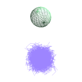
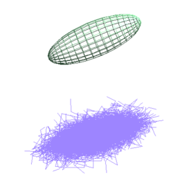
Figure 1: Equilibrium state (a) and non-equilibrium state (b). Top column shows statistical expression of collective deformation of polymer chains. Bottom column shows that one thousand polymer chains are superposed with fixing the center of mass.

III Fluid particle deformation

The anisotropic density distribution of polymer chains, discussed in the previous section, can be reflected to the macroscopic density distribution of fluid particle. In the conventional SPH MSPH , the density distribution of the $i$-th fluid particle $\rho_{i}(\boldsymbol{r})$ is isotropic and is obtained as follows:

$$\rho_{i}(\boldsymbol{r}) =m_{i}W(|\boldsymbol{r}-\boldsymbol{r}_{i}|,h),$$ (4)

$$W(|\boldsymbol{r}|,h) =\begin{cases}\frac{A_{d}}{(h\sqrt{\pi})^{d}}\left(e^{-|\boldsymbol{r}|^{2}/h^{2}}-e^{-4}\right),&\quad|\boldsymbol{r}|\leq 2h,\\ 0,&\quad|\boldsymbol{r}|>2h,\\ \end{cases}$$ (5)

where $m_{i}$ is the mass of $i$-th fluid particle, $W$ is the kernel function, $h$ is the width of the kernel $W$. $A_{d}$ is the normalization factor in $d$-dimensional space to satisfy $\int_{|\boldsymbol{r}|\leq 2h}{\rm d}\boldsymbol{r}W(|\boldsymbol{r}|,h)=1$ MSPH . In the conventional SPH, the fluid is assumed to be a Newtonian fluid which is an isotropic fluid. However, the polymer melt is not isotropic as shown in the previous section. The fluid particle of polymer melt should be anisotropic according to the distribution of polymer chains. The anisotropic density distribution can be produced by the following kernel:

$$W(\{r_{\alpha}\},\{\epsilon_{\alpha}\},h) =\begin{cases}\frac{A_{d}}{(h\sqrt{\pi})^{d}(\Pi_{\alpha=1}^{d}\epsilon_{\alpha})}\left(\Pi_{\alpha=1}^{d}e^{-r_{\alpha}^{2}/(\epsilon_{\alpha}h)^{2}}-e^{-4}\right),&\quad\sum_{\alpha=1}^{d}\left(\frac{r_{\alpha}}{\epsilon_{\alpha}}\right)^{2}\leq 4h^{2},\\ 0,&\quad\sum_{\alpha=1}^{d}\left(\frac{r_{\alpha}}{\epsilon_{\alpha}}\right)^{2}>4h^{2},\\ \end{cases}$$ (6)

where $\{\epsilon_{\alpha}\}$ is the ratio of semiaxis to the radius of the sphere and is a dimensionless variable. Equation (6) corresponds to Eq. (5) when $\epsilon_{\alpha}=1.$ If we assume an affinity to the density distribution of a fluid particle and the density distribution of the polymer chains in the fluid particle, $\epsilon_{\alpha}\equiv\overline{R}_{\alpha}/R_{\rm g}$. This assumption is reasonable because the macroscopic resolution is nearly equal to $h$ in this multiscale simulation and $h$ is much larger than the polymer chain length in the fluid particle. Higher order deformation at microscopic level is ignorable in the multiscale simulation.

Figure 2 shows the density distribution of a fluid particle on $z=0$ plane, obtained from Eqs. (4) and (6). The mass center of fluid particle is fixed to be $(0,0,0)$. Figures 2 (a) and (b) correspond to Figs 1 (a) and (b), respectively. The following parameters are assumed: $m=1.0[{\rm M}]$, $h=0.1[{\rm L}]$, $d=3$, $A_{3}=1.18516$ MSPH , where ${\rm M}$ is macroscopic mass unit and ${\rm L}(\neq a)$ is macroscopic length unit.

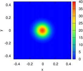
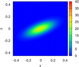
Figure 2: Density distribution of a fluid particle at equilibrium state (a) and non-equilibrium state (b) on $z=0$ plane.

IV Summary

We have considered the collective deformation of polymer chains in a flow field and derived a statistical way to describe the collective deformation by an ellipsoid. Then, we have connected this microscopic anisotropy to the macroscopic fluid particle. The anisotropy of fluid particle produces heterogeneity in the density distribution and will causes a flow to recover a uniform density distribution. This flow can produce ’Barus effect’ or ’die swell’ book.rheo which was not managed in the previous works MT2010 ; MT2011 ; MT2012 ; MYTY2013 . We expect that LMM will be improved with the techniques shown above and can solve an arbitrary polymer melt flow.

References

- (1) R. B. Bird, R. C. Armstrong and O. Hassager, Dynamics of polymeric liquids Vol. 1: Fluid mechanics, Wiley-Interscience, 1987.
- (2) R. B. Bird, C. F. Curtiss, R. C. Armstrong and O. Hassager, Dynamics of polymeric liquids Vol. 2: Kinetic theory, Wiley-Interscience, 1987.
- (3) K. Kremer and G. S. Grest, Dynamics of entangled linear polymer melts: A molecular dynamics simulation, J. Chem. Phys., 92, (1990), pp. 5057–5086.
- (4) C. C. Hua and J. D. Schieber, Segment connectivity, chain-length breathing, segmental stretch, and constraint release in reptation models. I. Theory and single-step strain predictions, J. Chem. Phys., 109, (1998), pp. 10018–10027.
- (5) Y. Masubuchi, J. Takimoto, K. Koyama, G. Ianniruberto, G. Marrucci, and F. Greco, Brownian simulations of a network of reptating primitive chains, J. Chem. Phys., 115, (2001), pp. 4387–4394.
- (6) M. Doi and J. Takimoto, Molecular modeling of entanglement, Phil. Trans. R. Soc. Lond. A, 361, (2003), pp. 641–652.
- (7) R. N. Khaliullin and J. D. Schieber, Self-Consistent Modeling of Constraint Release in a Single-Chain Mean-Field Slip-Link Model, Macromol., 42, (2009), pp. 7504–7517.
- (8) A. E. Likhtman, Single-Chain Slip-Link Model of Entangled Polymers: Simultaneous Description of Neutron Spin-Echo, Rheology, and Diffusion, Macromol., 38, (2005), pp. 6128–6139.
- (9) T. Uneyama, Single Chain Slip-Spring Model for Fast Rheology Simulations of Entangled Polymers on GPU, J. Soc. Rheol. Jpn., 39, (2011), pp. 135–152.
- (10) T. Uneyama and Y. Masubuchi, Multi-chain slip-spring model for entangled polymer dynamics, J. Chem. Phys., 137, (2012), pp. 154902(1–13).
- (11) M. Laso and H. C. Öttinger, Calculation of viscoelastic flow using molecular models: the CONNFFESSIT approach, J. Non-Newtonian Fluid Mech., 47, (1993), pp. 1–20.
- (12) C. C. Hua and J. D. Schieber, Application of kinetic theory models in spatiotemporal flows for polymer solutions, liquid crystals and polymer melts using the connffessit approach, Chem. Eng. Sci., 51, (1996), pp. 1473–1485.
- (13) W. Ren and W. E, Heterogeneous multiscale method for the modeling of complex fluids and micro-fluidics, J. Comp. Phys., 204, (2005), pp. 1–26.
- (14) S. De, J. Fish, M. S. Shephard, P. Keblinski, and S. K. Kumar, Multiscale modeling of polymer rheology, Phys. Rev. E, 74, (2006), pp. 030801(R)(1–4).
- (15) S. Yasuda and R. Yamamoto, Rheological properties of polymer melt between rapidly oscillating plates: An application of multiscale modeling, Europhys. Lett., 86, (2009), pp. 18002(1–5).
- (16) S. Yasuda and R. Yamamoto, Multiscale modeling and simulation for polymer melt flows between parallel plates, Phys. Rev. E, 81, (2010), pp. 036308(1–13).
- (17) T. Murashima and T. Taniguchi, Multiscale Lagrangian Fluid Dynamics Simulation for Polymeric Fluid, J. Polym. Sci. B, 48, (2010), pp. 886–893.
- (18) T. Murashima and T. Taniguchi, Multiscale simulation of history-dependent flow in entangled polymer melts, Europhys. Lett., 96, (2011), pp. 18002(1–6).
- (19) T. Murashima and T. Taniguchi, Flow-History-Dependent Behavior of Entangled Polymer Melt Flow Analyzed by Multiscale Simulation, J. Phys. Soc. Jpn., 81, (2012), pp. SA013(1–7).
- (20) T. Murashima, S. Yasuda, T. Taniguchi, and R. Yamamoto, Multiscale Modeling for Polymeric Flow: Particle-Fluid Bridging Scale Methods, J. Phys. Soc. Jpn., 82, (2013), pp. 012001(1–15).
- (21) J. J. Monaghan, Smoothed particle hydrodynamics, Rep. Prog. Phys., 68, (2005), pp. 1703–1759.
- (22) G. M. Zhang and R. C. Batra, Modified smoothed particle hydrodynamics method and its application to transient problems, Comp. Mech., 34, (2004), pp. 137-146.
- (23) J. Takimoto, PASTA (Polymer rheology Analyzer with Slip-link model of enTAnglement); software available at http://www.octa.jp/
- (24) D. V. Boger and K. Walters, Rheological Phenomena in Focus, Elsevier, 1993.