RESCEU-4/14,RUP-14-2

Investigating formation condition of primordial black holes for generalized initial perturbation profiles

Tomohiro Nakama

Department of Physics, Graduate School of Science,
The University of Tokyo, Bunkyo-ku, Tokyo 113-0033, Japan

Tomohiro Harada

Department of Physics, Rikkyo University, Toshima, Tokyo 175-8501, Japan

A. G. Polnarev

Astronomy Unit, School of Physics and Astronomy,
Queen Mary University of London,
Mile End Road, London E1 4NS, United Kingdom

Jun’ichi Yokoyama

Research Center for the Early Universe (RESCEU),
Graduate School of Science, The University of Tokyo,
Bunkyo-ku, Tokyo 113-0033, Japan

Kavli Institute for the Physics and Mathematics of the Universe (Kavli IPMU), WPI, TODIAS,
The University of Tokyo, Kashiwa, Chiba 277-8568, Japan

Primordial black holes (PBHs) are an important tool in cosmology to probe the primordial spectrum of small-scale curvature perturbations that reenter the cosmological horizon during radiation domination epoch. We numerically solve the evolution of spherically symmetric highly perturbed configurations to clarify the criteria of PBHs formation using a wide class of curvature profiles characterized by five parameters. It is shown that formation or non-formation of PBHs is determined essentialy by only two master parameters.

PRESENTED AT

The 10th International Symposium on Cosmology and Particle Astrophysics (CosPA2013)
Honolulu, Hawai’i, November 12–15, 2013

I introduction

It is well known that a region with large amplitude curvature profile can collapse to a primordial black hole (PBH) Zel’dovich and Novikov (1967); Hawking (1971). PBHs are formed soon after the region enters the cosmological horizon during the radiation-dominated epoch.

Even if PBHs would never have been detected, existing observational constraints Carr et al. (2010) will provide valuable information on inflationary cosmological models. It is important to probe the perturbation spectrum on significantly smaller scales as well in order to obtain more helpful information to single out the correct inflation model.

Originally the problem of PBH formation was studied analytically Carr and Hawking (1974); Carr (1975):

$$\frac{1}{3}\lesssim\overline{\delta}_{\mathrm{hc}},$$ (1)

where $\overline{\delta}_{\mathrm{hc}}$ is the energy density perturbation averaged over the overdense region evaluated at the time of horizon crossing. This criterion has long been used in papers on theoretical prediction of PBH abundance (but has recently been refined in Harada et al. (2013)). In this simple picture, the dependence on the profile or shape of perturbed regions has not been taken into account.

However, recent numerical analyses have shown that the condition for PBH formation does depend on the profile of perturbation Shibata and Sasaki (1999); Polnarev and Musco (2007) (see also Nadezhin et al. (1979); Niemeyer and Jedamzik (1999)). Both Shibata and Sasaki (1999) and Polnarev and Musco (2007)(hereafter PM) used two-parameter families of the initial profile and obtained two parametric conditions of PBH formation. It was clear from the above publications that one parametric description was not sufficient. However it was not clear whether the two-parametric description is good enough. In the present paper, we extend these preceding analyses by making many more numerical computations of PBH formation based on the initial curvature profile including many more parameters, adopting the five-parameter family of profiles. We show that the criterion of PBH formation can still be expressed in terms of two crucial (master) parameters, even though the considered profiles belong to the five-parametric family.

II Setting up the initial condition

The metric used can be written in the form used by Misner and Sharp Misner and Sharp (1964):

$$ds^{2}=-a^{2}dt^{2}+b^{2}dr^{2}+R^{2}(d\theta^{2}+\sin^{2}\theta d\phi^{2}),$$ (2)

where $R$, $a$ and $b$ are functions of $r$ and the time coordinate $t$. We consider a perfect fluid with the energy density $\rho(r,t)$ and pressure $P(r,t)$ and a constant equation-of-state parameter $\gamma$, $P(r,t)=\gamma\rho(r,t)$. We express the proper time derivative of $R$ as

$$U\equiv\frac{\dot{R}}{a},$$ (3)

with a dot denoting a derivative with respect to $t$.

We define the mass, sometimes referred to as the Misner-Sharp mass in the literature, within the shell of circumferential radius $R$ by

$$M(r,t)=4\pi\int^{R(r,t)}_{0}\rho(r,t)R^{2}dR.$$ (4)

We consider the evolution of a perturbed region embedded in a flat Friedmann-Lemaitre-Robertson-Walker (FLRW) Universe with metric

$$ds^{2}=-dt^{2}+S^{2}(t)(dr^{2}+r^{2}d\theta^{2}+r^{2}\sin^{2}\theta d\phi),$$ (5)

which is a particular case of (2). The scale factor in this background evolves as

$$S(t)=\left(\frac{t}{t_{\mathrm{i}}}\right)^{\alpha},\quad\alpha\equiv\frac{2}{3(1+\gamma)},$$ (6)

where $t_{\mathrm{i}}$ is some reference time.

The background Hubble parameter is

$$H_{0}(t)=\frac{\dot{R_{0}}}{a_{0}R_{0}}=\frac{\dot{S}}{S}=\frac{\alpha}{t}.$$ (7)

The energy density perturbation is defined as

$$\delta(t,r)\equiv\frac{\rho(t,r)-\rho_{0}(t)}{\rho_{0}(t)}.$$ (8)

The curvature profile $K(t,r)$ is defined by rewriting $b$ as

$$b(t,r)=\frac{R^{\prime}(t,r)}{\sqrt{1-K(t,r)r^{2}}}.$$ (9)

This quantity $K(t,r)$ vanishes outside the perturbed region so that the solution asymptotically approaches the background FLRW solution at spatial infinity.

We denote the comoving radius of a perturbed region by $r_{\mathrm{i}}$, the precise definition of which will be given later (see eq. (12)), and define a dimensionless parameter $\epsilon$ in terms of the square ratio of the Hubble radius $H_{0}^{-1}$ to the physical length scale of the configuration,

$$\epsilon\equiv\left(\frac{H_{0}^{-1}}{S(t)r_{\mathrm{i}}}\right)^{2}=(\dot{S}r_{\mathrm{i}})^{-2}=\frac{t_{\mathrm{i}}^{2\alpha}t^{\beta}}{\alpha^{2}r_{\mathrm{i}}^{2}},\quad\beta\equiv 2(1-\alpha).$$ (10)

When we set the initial conditions for PBH formation, the size of the perturbed region is much larger than the Hubble horizon. This means $\epsilon\ll 1$ at the beginning, so it can serve as an expansion parameter to construct an analytic solution of the system of Einstein equations to describe the spatial dependence of all the above variables at the initial moment when we set the initial conditions. In this paper, the second order solution, obtained in Polnarev et al. (2012) (hearafter PNY), is basically used to provide the initial conditions for the numerical computations.

We define the initial curvature profile as

$$K(0,r)\equiv K_{\mathrm{i}}(r),$$ (11)

where $K_{\mathrm{i}}(r)$ is an arbitrary function of $r$ which vanishes outside the perturbed region. We normalize radial Lagrangian coordinate $r$ in such a way that $K_{\mathrm{i}}(0)=1$.

In order to represent the comoving length scale of the perturbed region, we use the co-moving radius, $r_{\mathrm{i}}$, of the overdense region. We can calculate $r_{\mathrm{i}}$ by approximately solving (see PNY) the following equation for the energy density perturbation defined by (8):

$$\delta(t,r_{\mathrm{i}})=0.$$ (12)

III Two master parameters cruicial for PBHs formation

We now proceed to our full analysis (for more details, see Nakama et al. (2014)) introducing the following function

$$K_{\mathrm{i}}(r)=A\left[1+B\left(\frac{r}{\sigma_{1}}\right)^{2n}\right]\exp\left[-\left(\frac{r}{\sigma_{1}}\right)^{2n}\right]+(1-A)\exp\left[-\left(\frac{r}{\sigma_{2}}\right)^{2}\right],$$ (13)

which can represent various shapes of profiles using the five parameters as is shown in Figure 1. This function not only includes those investigated in previous work but also enables us to investigate new shapes of profiles.

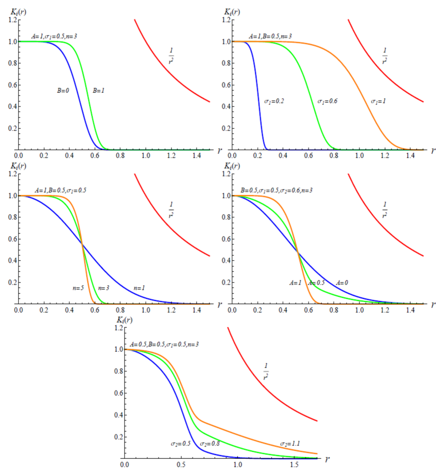
Figure 1: Dependence of the shapes of profiles represented by (13) on parameters. In each panel, the dependence of the shape on one of the parameters is shown with the rest of the parameters fixed.

It turned out that a relatively clear separation between configurations which collapse to PBHs and those which do not is obtained by the following combination:

$$\Delta\equiv r_{1/6}-r_{5/6}$$ (14)

and

$$I\equiv\int^{r_{3/5}}_{0}r^{2}K_{\mathrm{i}}(r)dr.$$ (15)

Figure 2 shows the results of numerical calculation with various initial conditions of the five-parameter family (13). Specifically we have chosen the values of model parameters in (13) in the range $0\leq A\leq 1$, $0\leq B\leq 1$, $\sigma_{\mathrm{min}}\leq\sigma_{1}\leq\sigma_{2}\leq\min\{2\sigma_{1},1.14/\sqrt{1-A}\}$, where $\sigma_{\mathrm{min}}$ is chosen to search only the profiles relevant to revealing the PBH formation condition and $n=1,2,3,4,5$. As is seen there the condition for PBH formation can be quite well described by the following fitting formula:

$$(S_{1}(\Delta-\Delta_{\mathrm{b}})+I_{\mathrm{b}})\Theta(-(\Delta-\Delta_{\mathrm{b}}))+(S_{2}(\Delta-\Delta_{\mathrm{b}})+I_{\mathrm{b}})\Theta(\Delta-\Delta_{\mathrm{b}})<I,$$ (16)

where $\Theta$ denotes the unit step function and $(S_{1},S_{2},\Delta_{\rm{b}},I_{\rm{b}})=(-0.021,-0.32,0.79,0.41)$, which represent the slopes of the two lines and the position of the break. This formula corresponds to the lower solid line in Figure 2.

Note that for the larger values of $\Delta$, the threshold value for PBH formation $I$ is smaller. This is because when $\Delta$ is larger, the pressure gradients are smaller and in addition gravity is relatively stronger even away from the centre, in which case gravity near the centre, measured by $I$, needs not be so large compared to cases with a smaller $\Delta$. Put differently, for $I\lesssim 0.43\equiv I_{\mathrm{cr}}$, profiles with a smaller $\Delta$ do not result in PBH formation because the pressure gradient is so large that the gravitational collapse is hindered. The dashed line in Figure 2 corresponds to the Carr’s condition eq.(1).

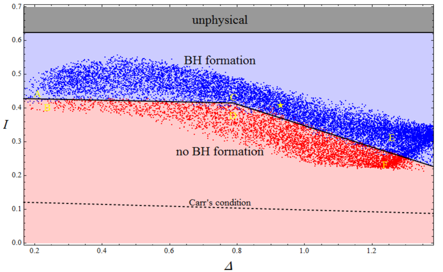
Figure 2: The PBH formation condition for the profiles represented by (13). The blue and red points correspond respectively to the profiles which lead to the black hole formation and those which do not. The shaded region labelled ”unphysical” corresponds to the profiles which do not satisfy $K_{\mathrm{i}}(r)<1/r^{2}$ and therefore are unphysical. The profile used as an example of the PBH-forming cases in this paper corresponds to the yellow star in this figure. The dashed line corresponds to the Carr’s condition.

IV Conclusion

In this paper we have presented the results of numerical computations of the time evolution of a perturbed region after the horizon re-entry. The initial conditions for these numerical computations were given using an analytical asymptotic expansion technique developed in our previous paper. By calculating the time evolution of various initial perturbations, the condition for PBH formation has been investigated. We have extended preceding analyses by performing many more numerical computations of PBH formation based on the initial curvature profiles characterized by five parameters which not only reproduce the variety of profiles near the centre but also incorporate the possible extended features in the tail region (see eq.(13)).

We have shown that the criterion of PBHs formation can still be expressed in terms of two crucial (master) parameters which correspond to the averaged amplitude of over density in the central region and the width of transition region at outer boundary. As is shown in Figure 2, this is the case even though our profiles are characterized by as many as five parameters. We have also provided a reliable physical interpretation of the two-parametric criterion.

ACKNOWLEDGEMENTS

This work was partially supported by JSPS Grant-in-Aid for Scientific Research 23340058 (J.Y.), Grant-in-Aid for Scientific Research on Innovative Areas No. 21111006 (J.Y.), Grant-in-Aid for Exploratory Research No. 23654082(T.H.), and Grant-in-Aid for JSPS Fellow No. 25.8199 (T.N.). TN thanks School of Physics and Astronomy, Queen Mary College, University of London for hospitality received during this work. We thank B. J. Carr for useful communications. TN acknowledges H. Kodama, K. Kohri, K. Ioka and H. Takami for helpful comments.

References

- Zel’dovich and Novikov (1967) Y. B. Zel’dovich and I. D. Novikov, Sov. Astron. 10, 602 (1967).
- Hawking (1971) S. Hawking, Mon. Not. Roy. Astron. Soc. 152, 75 (1971).
- Carr et al. (2010) B. Carr, K. Kohri, Y. Sendouda, and J. Yokoyama, Phys. Rev. D 81, 104019 (2010), eprint 0912.5297.
- Carr and Hawking (1974) B. J. Carr and S. Hawking, Mon. Not. Roy. Astron. Soc. 168, 399 (1974).
- Carr (1975) B. J. Carr, Astrophys. J. 201, 1 (1975).
- Harada et al. (2013) T. Harada, C.-M. Yoo, and K. Kohri (2013), eprint 1309.4201.
- Shibata and Sasaki (1999) M. Shibata and M. Sasaki, Phys. Rev. D 60, 084002 (1999), eprint gr-qc/9905064.
- Polnarev and Musco (2007) A. G. Polnarev and I. Musco, Class. Quant. Grav. 24, 1405 (2007), eprint gr-qc/0605122.
- Nadezhin et al. (1979) D. K. Nadezhin, I. D. Novikov, and A. G. Polnarev, NASA STI/Recon Technical Report N 80, 10983 (1979).
- Niemeyer and Jedamzik (1999) J. C. Niemeyer and K. Jedamzik, Phys. Rev. D 59, 124013 (1999), URL http://link.aps.org/doi/10.1103/PhysRevD.59.124013.
- Misner and Sharp (1964) C. W. Misner and D. H. Sharp, Phys. Rev. 136, B571 (1964).
- Polnarev et al. (2012) A. Polnarev, T. Nakama, and J. Yokoyama, J. Cosmol. Astropart. Phys. 2012, 027 (2012), URL http://stacks.iop.org/1475-7516/2012/i=09/a=027.
- Nakama et al. (2014) T. Nakama, T. Harada, A. Polnarev, and J. Yokoyama, Journal of Cosmology and Astroparticle Physics 2014, 037 (2014), URL http://stacks.iop.org/1475-7516/2014/i=01/a=037.