The van der Waals interaction in one, two, and three dimensions

Abstract

The van der Waals interaction between two polarizable atoms is considered. In three dimensions the standard form with an attractive $1/|{\mathbf{R}}|^{6}$ potential is obtained from second-order quantum perturbation theory. When the electron motion is restricted to lower dimensions (but the $1/|{\mathbf{R}}|$ Coulomb potential is retained), new terms in the expansion appear and alter both the sign and the $|{\mathbf{R}}|$ dependence of the interaction.

I Introduction

One of the most beautiful applications of perturbation theory in quantum mechanics is the computation of the van der Waals force between two atoms. The very existence of this force is perhaps surprising, because it arises even when both atoms are electrically neutral, resulting from the fact that the two atoms polarize each other. The simplest example is the interaction between two hydrogen atoms. If the two atoms are far apart the interaction between them is negligible and in the ground state the electron wave functions are spherically symmetric. As the two atoms approach each other a correlation between the atomic states arises, causing the van der Waals force. At leading order in the inverse distance between the atoms this is a dipole-dipole interaction. For a general introduction see Refs. TMF, ; Milton, ; SKSF, .

The computation of the strength of the van der Walls interaction is a classic problem in quantum mechanics. The problem was originally treated in Refs. EL, ; London, ; London2, , and can be formulated as follows:

Two hydrogen atoms are separated by a distance $|{\mathbf{R}}|$; see Fig. 1. Use perturbation theory to compute the correction to the ground state energy of the system due to the atoms’ polarizability, for large values of $|{\mathbf{R}}|$.

The problem is particularly appealing from the pedagogical perspective. It challenges the student to understand the central concepts of perturbation theory in a physically relevant case: What is the unperturbed system? What is perturbing Hamiltonian? What order in the perturbation is needed, and how large must $|{\mathbf{R}}|$ be in order for the results to apply?

Versions of the above problem are standard in quantum mechanics references.LL ; Schiff ; Sakurai ; Kittel ; BJ ; Abers ; Griffiths ; Holstein ; Stone ; AM ; Patterson ; Born In order to make the problem less technical for the students, it is tempting to simplify the computations by constraining the motion of the electrons to one or two dimensions, Kittel ; Griffiths ; Holstein ; Stone ; Patterson ; Born while keeping the $1/|{\mathbf{R}}|$ Coulomb interaction between the “atoms” (we will continue to use the word “atom” even when electrons are constrained to lower dimensions). Here we point out that this reduction also offers a good opportunity to discuss one of the common pitfalls of perturbation theory, namely the potential inconsistency of the perturbation series; this pitfall appears to have been overlooked in Refs. Born, ; Kittel, ; Patterson, ; Griffiths, ; Holstein, ; Stone, .

The consistency of the perturbation series comes into play because the problem contains two expansions: that of the interaction Hamiltonian and that of (quantum mechanical) perturbation theory. The interaction Hamiltonian is given by the Coulomb interaction between the two atoms (each consisting of an electron and a nucleus). This interaction vanishes rapidly for large $|{\mathbf{R}}|$ because both atoms are neutral. It is therefore natural to expand the interaction Hamiltonian in inverse powers of $|{\mathbf{R}}|$ (this can be understood as a multipole expansion). The leading-order term in the expansion of the interaction Hamiltonian is of order $1/|{\mathbf{R}}|^{3}$, and the familiar van der Waals term of order $1/|{\mathbf{R}}|^{6}$ arises in perturbation theory from the second-order contribution of this $1/|{\mathbf{R}}|^{3}$ term. Because the first-order contribution from the $1/|{\mathbf{R}}|^{3}$ term is zero, it is tempting to conclude that the familiar van der Waals term of order $1/|{\mathbf{R}}|^{6}$ is the leading term in the perturbative expansion.

However, as we will show in detail below, the $1/|{\mathbf{R}}|^{5}$ term of the perturbing Hamiltonian has a non-vanishing ground-state expectation value in one and two dimensions. This results in a leading term of order $1/|{\mathbf{R}}|^{5}$. We stress again that this is still for a $1/|{\mathbf{R}}|$ interaction. Only in three dimensions, as explicitly noted by Refs. EL, ; LL, ; Schiff, ; Sakurai, , does the ground-state expectation value of the $1/|{\mathbf{R}}|^{5}$ term of the perturbing Hamiltonian vanish, so the leading term is the second-order correction due to the $1/|{\mathbf{R}}|^{3}$ term of the perturbing Hamiltonian. The standard $1/|{\mathbf{R}}|^{6}$ dependence of the van der Waals interaction is therefore special to three dimensions.

Figure 1: The nuclei of two hydrogen atoms, indicated by the dots, are placed a distance $|{\mathbf{R}}|$ apart. The associated positions of the electrons are at the end of the vectors ${\mathbf{r}}_{A}$ and ${\mathbf{r}}_{B}$. While each atom is electrically neutral their polarizability gives rise to the van der Waals interaction.

II The system

We consider the nuclei of the atoms fixed, so the Hilbert space is just the product of the Hilbert space of each electron:

$$\mathcal{H}=\mathcal{H}_{A}\otimes\mathcal{H}_{B}=L^{2}(\mathbb{R}^{d})\otimes L^{2}(\mathbb{R}^{d}),$$ (1)

where $d\geq 1$ is the number of space dimensions that the electrons are allowed to explore. The total Hamiltonian is

$$H=H_{0}+H_{I},\qquad H_{0}=H_{A}+H_{B},$$ (2)

where $H_{A}$ and $H_{B}$ describe the two atoms and the interaction isNote1

$$H_{I}=k\left(\frac{1}{|{\mathbf{R}}|}+\frac{1}{|{\mathbf{R}}-{\mathbf{r}}_{A}+{\mathbf{r}}_{B}|}-\frac{1}{|{\mathbf{R}}-{\mathbf{r}}_{A}|}-\frac{1}{|{\mathbf{R}}+{\mathbf{r}}_{B}|}\right),$$ (3)

with

$$k=\frac{e^{2}}{4\pi\epsilon_{0}}.$$ (4)

(See Fig. 1.) In three dimensions this is the standard form of the Coulomb interaction. Let us emphasize that we do not assume that the atom Hamiltonians $H_{A}$ and $H_{B}$ are of the usual hydrogen form (see also the discussion around Eq. (22)).

Below we consider also the situation where the motion of the electrons is confined to one or two dimensions, but we keep the form of the interaction Hamiltonian. In other words the electromagnetic field is always allowed to explore all three spatial dimensions.

Note that we ignore the fermionic nature of the electrons. The model therefore makes sense only when $|{\mathbf{R}}|$ is much larger than the size of the atoms, so the overlap of the electron wavefunctions is negligible. Instead of hydrogen atoms, we could more generally consider single-valence-electron atoms, i.e., (neutral) atoms with a single electron outside a closed shell.

Since the general form of the van der Waals interaction in one, two, and three dimensions follows from the symmetries, we do not need the explicit form of $H_{A}$ and $H_{B}$. Rather we simply assume that $H_{A}$ and $H_{B}$ have rotational symmetry. In more detail, let $U_{M,A}$ be the unitary rotation operator defined by

$$(U_{M,A}\psi)({\mathbf{r}}_{A},{\mathbf{r}}_{B})=\psi(M{\mathbf{r}}_{A},{\mathbf{r}}_{B}),$$ (5)

where $M$ is an $SO(d)$ matrix for $d\geq 2$, and for $d=1$ we set $M=\pm 1$. By rotational symmetry we mean that $U_{M,A}$ (and the corresponding $U_{M,B}$) commutes with $H_{0}$. We further assume that the ground state $\psi_{0}$ (we will also use the notation $|0\rangle$) of $H_{0}$ is unique (and that degeneracies due to other degrees of freedom, like spin, are irrelevant). It follows that

$$|\psi_{0}(M{\mathbf{r}}_{A},M^{\prime}{\mathbf{r}}_{B})|=|\psi_{0}({\mathbf{r}}_{A},{\mathbf{r}}_{B})|.$$ (6)

For notational simplicity we assume that the two atoms are identical.

Before we proceed with the calculation, let us note that for sufficiently large $|{\mathbf{R}}|$ the form of the interaction (3) is modified by QED effects.CP We will not discuss this complication further, but refer the interested reader to, for example, Ref. Holstein, .

III General form of the van der Waals interaction

To derive the form of the van der Waals interaction we will assume that $|{\mathbf{R}}|$ is sufficiently large and compute the correction to the ground state energy using perturbation theory. As mentioned in the introduction this is a standard problem in quantum mechanics, see e.g. Refs. LL, ; Schiff, ; Sakurai, ; Kittel, ; BJ, ; Abers, ; Griffiths, ; Holstein, ; Stone, ; AM, ; Born, ; Patterson, , however when constraining the motion of the electrons to one or two dimensions the nature of the interaction changes. First we will show how the familiar $1/|{\mathbf{R}}|^{6}$ term arises and subsequently, by carefully checking the consistency of the perturbative expansion, we will show that in one and two dimensions the $1/|{\mathbf{R}}|^{6}$ term is subleading.

III.1 The familiar $1/|{\mathbf{R}}|^{6}$ form

To calculate the correction to the ground state energy of the full system, we expand $H_{I}$ in powers of $1/|{\mathbf{R}}|$. The leading term is of order $1/|{\mathbf{R}}|^{3}$

$$H_{I}=k\frac{({\mathbf{r}}_{A}\cdot{\mathbf{r}}_{B})|{\mathbf{R}}|^{2}-3({\mathbf{R}}\cdot{\mathbf{r}}_{A})({\mathbf{R}}\cdot{\mathbf{r}}_{B})}{|{\mathbf{R}}|^{5}}+O(|{\mathbf{R}}|^{-4}).$$ (7)

Let us choose coordinates such that ${\mathbf{R}}$ points along the $x$-axis. Since we have assumed that the ground state is unique we may simply plug this into the standard formula for the first order correction. We then find ($E_{n}$ denotes the energy levels of the unperturbed Hamiltonian $H_{0}$)

$$\Delta_{1}E_{0}=\frac{k}{|{\mathbf{R}}|^{3}}\langle 0|{\mathbf{r}}_{A}\cdot{\mathbf{r}}_{B}-3x_{A}x_{B}|0\rangle+O(|{\mathbf{R}}|^{-4}).$$ (8)

Here $|0\rangle$ is the ground state of $H_{0}=H_{A}+H_{B}$ which has the product form

$$|0\rangle=|0_{A}\rangle|0_{B}\rangle,$$ (9)

and by rotational symmetry, we have

$$\langle 0_{A}|{\mathbf{r}}_{A}|0_{A}\rangle=\langle 0_{B}|{\mathbf{r}}_{B}|0_{B}\rangle=\mathbf{0}.$$ (10)

Thus

$$\Delta_{1}E_{0}=0+O(|{\mathbf{R}}|^{-4}).$$ (11)

Let us go on to the second order correction due to the $1/|{\mathbf{R}}|^{3}$ term in $H_{I}$:

$$\Delta_{2}E_{0} = -\sum_{n\neq 0}\frac{|\langle n|H_{I}|0\rangle|^{2}}{E_{n}-E_{0}}$$

$$= -\frac{k^{2}}{|{\mathbf{R}}|^{6}}\sum_{n\neq 0}\frac{|\langle n|{\mathbf{r}}_{A}\cdot{\mathbf{r}}_{B}-3x_{A}x_{B}|0\rangle|^{2}}{E_{n}-E_{0}}+O(|{\mathbf{R}}|^{-8}),$$

where $|n\rangle$ are the eigenstates of $H_{0}$. As we have indicated, there is no $1/|{\mathbf{R}}|^{7}$ term, see Appendix A for details. Now one might be satisfied, since we have reproduced the expected $1/|{\mathbf{R}}|^{6}$ attractive potential (note that the sum is positive), but as we shall now see the $1/|{\mathbf{R}}|^{6}$ is only the leading term in 3 spatial dimensions.

III.2 Consistency of the expansion and the difference between one, two and three dimensions

The second order correction, $\Delta_{2}E_{0}$, to the ground state energy we found is $O(|{\mathbf{R}}|^{-6})$. We used second order perturbation theory since the first order term vanished $\Delta_{1}E_{0}=0$. However, for the first order correction we used an expansion of the interaction Hamiltonian, Eq. (7), which only holds up to $O(|{\mathbf{R}}|^{-4})$. So in order to check the consistency of the expansion we should calculate the first order corrections also due to terms up to order $1/|{\mathbf{R}}|^{6}$ in $H_{I}$.

Instead of simply expanding $H_{I}$ and calculating the expectation value, we will follow a slightly indirect route, which will prove more enlightening (the completely equivalent standard approach is included in Appendix B). To this end, first note that

$$\Delta_{1}E_{0}=\langle 0|H_{I}|0\rangle=k\langle 0_{B}|V_{A}({\mathbf{R}})-V_{A}({\mathbf{R}}+{\mathbf{r}}_{B})|0_{B}\rangle,$$ (13)

with

$$V_{A}({\mathbf{r}})=\left\langle 0_{A}\middle|\frac{1}{|{\mathbf{r}}|}-\frac{1}{|{\mathbf{r}}-{\mathbf{r}}_{A}|}\middle|0_{A}\right\rangle.$$ (14)

Writing $V_{A}({\mathbf{r}})$ as

$$V_{A}({\mathbf{r}})=\int d^{d}{\mathbf{r}}_{A}\frac{\delta^{d}({\mathbf{r}}_{A})-|\psi_{0,A}({\mathbf{r}}_{A})|^{2}}{|{\mathbf{r}}-{\mathbf{r}}_{A}|},$$ (15)

it is clear that it is (proportional to) the electrostatic potential of the ground state of the $A$ atom.

We expand (this is just the familiar multipole expansion),

$$V_{A}({\mathbf{r}})=\left\langle 0_{A}\middle|-\frac{{\mathbf{r}}\cdot{\mathbf{r}}_{A}}{|{\mathbf{r}}|^{3}}+\frac{|{\mathbf{r}}_{A}|^{2}}{2|{\mathbf{r}}|^{3}}-\frac{3({\mathbf{r}}\cdot{\mathbf{r}}_{A})^{2}}{2|{\mathbf{r}}|^{5}}+O(|{\mathbf{r}}|^{-4})\middle|0_{A}\right\rangle$$ (16)

and using

$$\langle 0_{A}||{\mathbf{r}}_{A}|^{2}|0_{A}\rangle=\frac{d\langle 0_{A}|({\mathbf{r}}\cdot{\mathbf{r}}_{A})^{2}|0_{A}\rangle}{|{\mathbf{r}}|^{2}}$$ (17)

we find that in general (note that $V_{A}$ only depends on $|{\mathbf{r}}|$ by rotation symmetry)

$$V_{A}({\mathbf{r}})=-\frac{(3-d)a^{2}}{2}\frac{1}{|{\mathbf{r}}|^{3}}+O(|{\mathbf{r}}|^{-5}).$$ (18)

Here the characteristic length $a$ is defined by

$$a^{2}=\frac{\langle 0_{A}||{\mathbf{r}}_{A}|^{2}|0_{A}\rangle}{d}.$$ (19)

Any $|{\mathbf{r}}|^{-4}$ term in (16) would have to contain three factors of ${\mathbf{r}}_{A}$, and would thus vanish by the inversion symmetry.

We now plug the result for $V_{A}$ into (13), and find

$$\Delta_{1}E_{0}=-\frac{3(3-d)ka^{2}}{2}\left\langle 0_{B}\middle|\frac{{\mathbf{R}}\cdot{\mathbf{r}}_{B}}{|{\mathbf{R}}|^{5}}+\frac{|{\mathbf{r}}_{B}|^{2}}{2|{\mathbf{R}}|^{5}}-\frac{5({\mathbf{R}}\cdot{\mathbf{r}}_{B})^{2}}{2|{\mathbf{R}}|^{7}}+O(|{\mathbf{R}}|^{-6})\middle|0_{B}\right\rangle,$$ (20)

so the general first order correction takes the form (even negative powers again vanish by inversion symmetry)

$$\Delta_{1}E_{0}=\frac{3(3-d)(5-d)k}{4}\frac{a^{4}}{|{\mathbf{R}}|^{5}}+O(|{\mathbf{R}}|^{-7}).$$ (21)

For the standard derivation of this result see Appendix B. We conclude that for $d=1,2$ a repulsive $1/|{\mathbf{R}}|^{5}$ term is present, which we had missed before. However, for $d=3$ the leading term is indeed the $1/|{\mathbf{R}}|^{6}$ term. This demonstrates the importance of the consistency of the expansion.Note2

The $1/|{\mathbf{R}}|^{5}$ will also become the dominant term in 3 spatial dimensions provided that we consider corrections to excited states of the atoms (degeneracies can even change it to $1/|{\mathbf{R}}|^{3}$), see e.g. Refs. LL, and Abers, .

In the preceding discussion we have tacitly assumed that $a^{2}>0$ such that the $1/|{\mathbf{r}}|^{3}$ term in $V_{A}({\mathbf{r}})$ is non-zero, cf. Eq. (18). Is it possible to come up with (singular) models that violate this? If we let the atom Hamiltonian take the hydrogen like form

$$H_{A}=-\frac{\hbar}{2m}\frac{d^{2}}{dx_{A}^{2}}-\frac{k}{|x_{A}|}$$ (22)

in $d=1$ the ground state wavefunction becomes completely localized at $x_{A}=0$, see Ref. Loudon, . We thus have $a^{2}=0$ and hence no $1/|{\mathbf{R}}|^{5}$ correction to $E_{0}$. In the following we will focus on the generic $a^{2}>0$ situation.

IV Geometrical interpretation

We have seen that that $V_{A}({\mathbf{r}})=0+O(|{\mathbf{r}}|^{-5})$ for $d=3$. There is a simple way to understand this. Consider a rotationally symmetric distribution $\rho$ in $d=3$ with bounded support, in the sense that $\rho({\mathbf{r}})=0$ for $|{\mathbf{r}}|>r_{*}$. From electrostatics we know that

$$\int d^{3}{\mathbf{r}}^{\prime}\frac{\rho(|{\mathbf{r}}^{\prime}|)}{|{\mathbf{r}}-{\mathbf{r}}^{\prime}|}=\frac{q}{|{\mathbf{r}}|},\qquad q=\int d^{3}{\mathbf{r}}^{\prime}\rho(|{\mathbf{r}}^{\prime}|)$$ (23)

when $|{\mathbf{r}}|>r_{*}$. Looking back at (15), it follows immediately that (in $d=3$)

$$V_{A}({\mathbf{r}})=\frac{1}{|{\mathbf{r}}|}-\frac{1}{|{\mathbf{r}}|}=0$$ (24)

as long as ${\mathbf{r}}$ is outside the atom. Under the assumption that electron wavefunctions of the two atoms don’t overlap (which is necessary for the consistency of the model anyway), we conclude that the first order correction $\Delta_{1}E_{0}$ vanishes to all orders in $|{\mathbf{R}}|^{-1}$ in $d=3$. This can also be understood in terms of the orthogonality properties of the spherical harmonics, see e.g. Refs. Schiff, and Sakurai, . (Of course, for physically realistic wavefunctions there will be some overlap, but it will fall off at least as fast as $\exp(-|{\mathbf{R}}|/a)$, which will not show up in an expansion in $1/|{\mathbf{R}}|$, see Ref. LL, .)

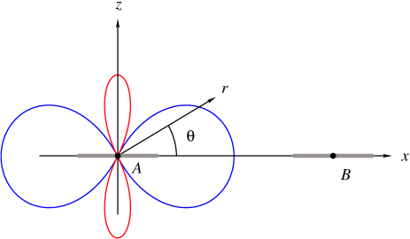
Figure 2: The one dimensional system embedded in three dimensional space. Here we only show the $xz$ plane. The one dimensional electron ‘clouds’ are indicated by the horizontal gray lines. A polar plot of (26) shows the shape of the $A$ atom’s quadrupole. On the two lobes along the $z$-axis $V_{A}({\mathbf{r}})$ is positive, while it is negative on the lobes along the $x$-axis. For the two dimensional system the picture would be similar, but with the electron clouds forming discs in the $xy$ plane.

To understand why the atoms repel each other for $d<3$ it is useful to think of the system as embedded in three dimensional space. It is then meaningful to ask what the potential $V_{A}({\mathbf{r}})$ is, if ${\mathbf{r}}$ is allowed to be a three dimensional vector. Let us set

$${\mathbf{r}}=|{\mathbf{r}}|(\hat{\mathbf{x}}\cos\theta+\hat{\mathbf{z}}\sin\theta),$$ (25)

where $\hat{\mathbf{x}}$ is a unit vector parallel to the system, while $\hat{\mathbf{z}}$ is perpendicular to the system, see Figure 2. If we plug (25) into (16) we find

$$V_{A}({\mathbf{r}})=-\frac{(3\cos^{2}\theta-d)a^{2}}{2}\frac{1}{|{\mathbf{r}}|^{3}}+O(|{\mathbf{r}}|^{-5}),\qquad\text{for $d=1,2$},$$ (26)

which reduces to (18) when $\theta=0$ (or $\theta=\pi$) as it should. We recognize the leading term as the potential of a quadrupole (the symmetry of the problem excludes the appearance of dipoles). In the model the quadrupoles of the atoms are aligned such that they will repel each other. The repulsion can thus be understood as the result of the permanent quadrupole moments of the atoms.

V The Drude model

Above we have provided the general from of the van der Waals interaction based on symmetry arguments. Here we exemplify the general results in a simple model for the atoms: the Drude model. In the Drude model, see e.g. Refs. Kittel, ; Griffiths, ; Stone, ; Born, ; London2, ; Patterson, ; Holstein, , the electrons are bound by a harmonic potential,

$$H_{A}=-\frac{\hbar\nabla^{2}_{A}}{2m}+\frac{1}{2}m\omega^{2}|{\mathbf{r}}_{A}|^{2},\qquad H_{B}=-\frac{\hbar\nabla^{2}_{B}}{2m}+\frac{1}{2}m\omega^{2}|{\mathbf{r}}_{B}|^{2}.$$ (27)

If we only keep the leading term of $H_{I}$ given in Eq. (7), the Drude model remains harmonic, and we can write down the ‘exact’ correction to the ground state energy, see e.g. Refs. Kittel, ; Griffiths, ; Stone, ; Born, ; London2, ; Patterson, ; Holstein, . To do this one changes coordinates to ${\mathbf{r}}_{\pm}=({\mathbf{r}}_{A}\pm{\mathbf{r}}_{B})/\sqrt{2}$. In terms of ${\mathbf{r}}_{\pm}$ the model (with the truncated $H_{I}$) is just $2d$ decoupled oscillators, and the ground state energy is

$$\Delta E_{0}=\frac{\hbar}{2}\left(\tilde{\omega}_{2}+\tilde{\omega}_{-2}+(d-1)(\tilde{\omega}_{1}+\tilde{\omega}_{-1})-2d\tilde{\omega}_{0}\right),$$ (28)

with the shifted frequencies (note that $k=e^{2}/4\pi\epsilon_{0}$ is not the spring constant)

$$\tilde{\omega}_{n}^{2}=\omega^{2}+\frac{nk}{m|{\mathbf{R}}|^{3}}.$$ (29)

If we expand (28) in $1/|{\mathbf{R}}|$ we obtain (there is no $1/|{\mathbf{R}}|^{3}$ or $1/|{\mathbf{R}}|^{9}$ term because (28) is symmetric under $|{\mathbf{R}}|\to-|{\mathbf{R}}|$)

$$\Delta E_{0}=-\frac{(3+d)k^{2}a^{4}}{2\hbar\omega}\frac{1}{|{\mathbf{R}}|^{6}}+O(|{\mathbf{R}}|^{-12}).$$ (30)

Here $a$, as defined by (19), is

$$a^{2}=\frac{\hbar}{2m\omega}.$$ (31)

It is easy to check that we get the same result from (III.1), i.e. from the second order correction due to the $1/|{\mathbf{R}}|^{3}$ term in $H_{I}$. In 3 dimensions this is thus completely self consistent and provides the leading order correction due to the interaction between the two neutral atoms. However, in one and two dimensions, as we have seen above, the leading term is of order $1/|{\mathbf{R}}|^{5}$: The general form of the leading corrections to the Drude ground state energy is

$$\Delta E_{0}=\frac{3(3-d)(5-d)k}{4}\left(\frac{a^{4}}{|{\mathbf{R}}|^{5}}+\frac{5(7-d)a^{6}}{2|{\mathbf{R}}|^{7}}\right)-\frac{(3+d)k^{2}a^{4}}{2\hbar\omega}\frac{1}{|{\mathbf{R}}|^{6}}+O(|{\mathbf{R}}|^{-8}).$$ (32)

Here we have included the $1/|{\mathbf{R}}|^{7}$ term, see Appendix C for details.

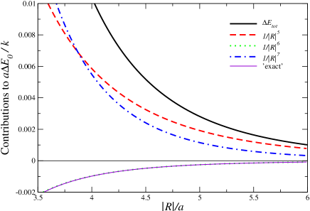
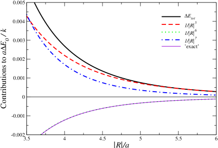
Figure 3: The corrections to the ground state energy in the Drude model left: in 1 dimension right: in 2 dimensions. The thick line shows the total correction up to order $1/\tilde{R}^{7}$. The curve labeled ‘exact’ is a plot of Eq. (28). The contributions from the terms of order $1/\tilde{R}^{5}$ (the dashed lines) are dominant for $\tilde{R}\gtrsim 5$. Note that the ‘exact’ curve is indistinguishable from $1/\tilde{R}^{6}$ curve in both plots. This is to be expected since they only start to differ at $O(\tilde{R}^{-12})$, see Eq. (30).

To get a feeling for the magnitude of the different terms, let us choose $m$ to be the electron mass, $m_{e}$, and $a$ to be the Bohr radius

$$a=a_{\text{Bohr}}=\frac{\hbar^{2}}{m_{e}k}.$$ (33)

Using (31) we then have

$$\frac{a\Delta E_{0}}{k}=\frac{3(3-d)(5-d)}{4}\left(\frac{1}{\tilde{R}^{5}}+\frac{5(7-d)}{2}\frac{1}{\tilde{R}^{7}}\right)-(3+d)\frac{1}{\tilde{R}^{6}}+O(\tilde{R}^{-8}),$$ (34)

where the dimensionless separation is

$$\tilde{R}=\frac{|{\mathbf{R}}|}{a}.$$ (35)

The correction is plotted in Figure 3 for one and two dimensions. Note that we should only trust our perturbative calculations in the region where the ‘leading’ $1/|{\mathbf{R}}|^{5}$ correction dominates the other corrections, i.e. for $\tilde{R}\gtrsim 5$.

VI Conclusion

The van der Waals interaction between two neutral atoms offers a perfect exercise in quantum mechanics. It allows the student to gain experience with the basic concepts of perturbation theory in a physically relevant case. The problem also naturally suggests itself to discuss more advanced concepts such as retardation.Holstein Here we have used the van der Waals interaction to emphasize the importance of the consistency of the perturbation series. In particular, we have shown that when the electron motion is restricted to one and two dimensions the ordering of of the perturbative series is different from the familiar form obtained in three spatial dimensions. This affects the $|{\mathbf{R}}|$-dependence of the van der Waals interaction which becomes a repulsive and of order $1/|{\mathbf{R}}|^{5}$ in one and two dimensions. This pitfall offers a great chance to discuss the importance of the consistency of the perturbation series and appears to have been overlooked in the literature.Kittel ; Griffiths ; Holstein ; Stone

The presentation has been based almost entirely on symmetry arguments. Explicit evaluation of the perturbation series has been presented for the Drude model. We hope that this discussion may serve as inspiration also at other universities and colleges.

Appendix A No $1/|{\mathbf{R}}|^{7}$ dependence of $\Delta_{2}E_{0}$

Here we explain why a $1/|{\mathbf{R}}|^{7}$ dependence is excluded from $\Delta_{2}E_{0}$ in Eq. (III.1). Consider the unitary inversion operator, $\mathcal{I}$, defined by

$$(\mathcal{I}\psi)({\mathbf{r}}_{A},{\mathbf{r}}_{B})=\psi(-{\mathbf{r}}_{A},-{\mathbf{r}}_{B}).$$ (36)

It is clear that

$$\mathcal{I}{\mathbf{r}}_{A/B}\mathcal{I}=-{\mathbf{r}}_{A/B},\qquad\mathcal{I}^{2}=\mathds{1}.$$ (37)

Now $\mathcal{I}$ commutes with $H_{0}$,Note3 which means that we can assume that the $|n\rangle$ are also eigenstates of $\mathcal{I}$. We can thus split the sum in (III.1) as

$$\Delta_{2}E_{0}=-\sum_{\begin{subarray}{c}n\neq 0\\ \mathcal{I}|n\rangle=+|n\rangle\end{subarray}}\frac{|\langle n|H_{I}|0\rangle|^{2}}{E_{n}-E_{0}}-\sum_{\begin{subarray}{c}n\neq 0\\ \mathcal{I}|n\rangle=-|n\rangle\end{subarray}}\frac{|\langle n|H_{I}|0\rangle|^{2}}{E_{n}-E_{0}}.$$ (38)

It is easy to see that the $|{\mathbf{R}}|^{-3}$ terms of $H_{I}$ will only contribute to the first sum, while the $|{\mathbf{R}}|^{-4}$ terms will only contribute to the second sum. Hence, a term of order $1/|{\mathbf{R}}|^{7}$ cannot result.

Appendix B Direct calculation of $\Delta_{1}E_{0}$

In Section III.2 we calculate the first order correction in an indirect way by first considering the potential $V_{A}({\mathbf{r}})$. Here we outline a more standard brute force derivation of (21). With ${\mathbf{R}}=|{\mathbf{R}}|\hat{\mathbf{x}}$ we expand $H_{I}$ to order $1/|{\mathbf{R}}|^{5}$:

$$k^{-1}H_{I}=[{\mathbf{r}}_{A}\cdot{\mathbf{r}}_{B}-3x_{A}x_{B}]\frac{1}{|{\mathbf{R}}|^{3}}\\ +\left[3({\mathbf{r}}_{A}\cdot{\mathbf{r}}_{B})(x_{A}-x_{B})+\frac{3}{2}(|{\mathbf{r}}_{A}|^{2}x_{B}-|{\mathbf{r}}_{B}|^{2}x_{A})+\frac{15}{2}x_{A}x_{B}(x_{B}-x_{A})\right]\frac{1}{|{\mathbf{R}}|^{4}}\\ +\Biggl{[}\frac{3}{2}({\mathbf{r}}_{A}\cdot{\mathbf{r}}_{B})\Bigl{(}({\mathbf{r}}_{A}\cdot{\mathbf{r}}_{B})-|{\mathbf{r}}_{A}|^{2}-|{\mathbf{r}}_{B}|^{2}\Bigr{)}+\frac{3}{4}|{\mathbf{r}}_{A}|^{2}|{\mathbf{r}}_{B}|^{2}+\frac{15}{4}\Bigl{(}2({\mathbf{r}}_{A}\cdot{\mathbf{r}}_{B})x_{A}^{2}+2({\mathbf{r}}_{A}\cdot{\mathbf{r}}_{B})x_{B}^{2}\\ -|{\mathbf{r}}_{A}|^{2}x_{B}^{2}-|{\mathbf{r}}_{B}|^{2}x_{A}^{2}+2|{\mathbf{r}}_{A}|^{2}x_{A}x_{B}+2|{\mathbf{r}}_{B}|^{2}x_{A}x_{B}-4({\mathbf{r}}_{A}\cdot{\mathbf{r}}_{B})x_{A}x_{B}\Bigr{)}\\ +\frac{35}{4}(3x_{A}^{2}x_{B}^{2}-2x_{A}^{3}x_{B}-2x_{B}^{3}x_{A})\Biggr{]}\frac{1}{|{\mathbf{R}}|^{5}}+O(|{\mathbf{R}}|^{-6}).$$ (39)

The first order correction to the ground state energy is the expectation value of this expanded operator in the unperturbed ground state $|0\rangle$ of Eq. (9). By inversion symmetry, the expectation value of all the $1/|{\mathbf{R}}|^{3}$ and $1/|{\mathbf{R}}|^{4}$ terms vanish. The non-zero expectation values are (note that these hold in general, not just for the Drude model)

$$\langle 0|({\mathbf{r}}_{A}\cdot{\mathbf{r}}_{B})^{2}|0\rangle =da^{4}, \langle 0|({\mathbf{r}}_{A}\cdot{\mathbf{r}}_{B})x_{A}x_{B}|0\rangle =a^{4},$$ (40)

$$\langle 0||{\mathbf{r}}_{A}|^{2}|{\mathbf{r}}_{B}|^{2}|0\rangle =d^{2}a^{4}, \langle 0|x_{A}^{2}x_{B}^{2}|0\rangle =a^{4},$$ (41)

and

$$\langle 0||{\mathbf{r}}_{A}|^{2}x_{B}^{2}|0\rangle=\langle 0||{\mathbf{r}}_{B}|^{2}x_{A}^{2}|0\rangle=da^{4}.$$ (42)

In deriving these it is useful to note that e.g.

$$\langle 0|x_{A}y_{A}|0\rangle=0$$ (43)

by rotational symmetry. Combining the previous equations we obtain

$$\Delta_{1}E_{0}=\langle 0|H_{I}|0\rangle=\frac{3(3-d)(5-d)k}{4}\frac{a^{4}}{|{\mathbf{R}}|^{5}}+O(|R|^{-6}),$$ (44)

in agreement with (21). We observe that the first order correction is non vanishing in one and two dimensions.

Appendix C The $1/|{\mathbf{R}}|^{7}$ dependence of $\Delta_{1}E_{0}$

We first calculate the $1/|{\mathbf{r}}|^{5}$ term of $V_{A}({\mathbf{r}})$:

$$V_{A}({\mathbf{r}})=-\frac{(d-3)}{2}\left(\frac{a^{2}}{|{\mathbf{r}}|^{3}}+\frac{(d-5)\alpha a^{4}}{4|{\mathbf{r}}|^{5}}\right)+O(|{\mathbf{r}}|^{-7}),$$ (45)

where the positive coefficient $\alpha$ depends on the shape of the wave function and is defined by

$$\langle 0_{A}|x_{A}^{4}|0_{A}\rangle=\alpha a^{4}.$$ (46)

In the Drude model we have $\alpha=3$. To get the expression (45) for $d>1$ one needs the relation

$$\langle 0_{A}|x_{A}^{4}|0_{A}\rangle=3\langle 0_{A}|x_{A}^{2}y_{A}^{2}|0_{A}\rangle$$ (47)

which follows by doing the spherical integration, or by expanding the identity

$$\langle 0_{A}|x_{A}^{4}|0_{A}\rangle=\left\langle 0_{A}\middle|\left(\frac{x_{A}+y_{A}}{\sqrt{2}}\right)^{4}\middle|0_{A}\right\rangle.$$ (48)

Plugging (45) into (13) we obtain

$$\Delta_{1}E_{0}=\frac{(3-d)(5-d)k}{4}\left(\frac{3a^{4}}{|{\mathbf{R}}|^{5}}+\frac{5(7-d)\alpha a^{6}}{2|{\mathbf{R}}|^{7}}\right)+O(|{\mathbf{R}}|^{-9}).$$ (49)

References

• (1) M. M. Taddei, T. N. C. Mendes, and C. Farina, “An introduction to dispersive interactions,” Eur. J. Phys. 31, 89–99 (2010).
• (2) K. A. Milton, “Resource Letter VWCPF-1: van der Waals and Casimir-Polder forces,” Am. J. Phys. 79, 697–711 (2011).
• (3) R. de M. e Souza, W. J. M. Kort-Kamp, C. Sigaud and C. Farina, “Image method in the calculation of the van der Waals force between an atom and a conducting surface,” Am. J. Phys. 81, 366–376 (2013).
• (4) R. Eisenschitz and F. London, “Über das Verhältnis der van der Waalsschen Kräfte zu den homöopolaren Bindungskräften,” Z. Phys. 60, 491–527 (1930).
• (5) F. London, “Zur Theorie und Systematik der Molekularkräfte,” Z. Phys. 63, 245–279 (1930).
• (6) F. London, “The general theory of molecular forces,” Trans. Faraday Soc. 33, 8b–26 (1937).
• (7) L. D. Landau and E. M. Lifshitz, Quantum Mechanics (non-relativistic theory), third edition (Pergamon Press, Oxford, 1991).
• (8) L. I. Schiff, Quantum Mechanics, third edition (McGraw-Hill International, Tokyo, 1968).
• (9) J. J. Sakurai and J. Napolitano, Modern Quantum Mechanics, second edition (Pearson Education, Harlow, 2010).
• (10) N. W. Ashcroft and N. D. Mermin, Solid State Physics (Thomson Learning, Orlando, 1976).
• (11) B. H. Bransden and C.J. Joachin, Quantum Mechanics, second edition (Prentice Hall, Harlow, 2000).
• (12) E. S. Abers, Quantum Mechanics (Pearson Education, Prentice Hall, New Jersey, 2004).
• (13) M. Born, Atomic Physics, 8th. edition (Blake and Son Limited, Edinburgh, 1969).
• (14) J. D. Patterson and B.C. Baily, Solid-State Physics, Introduction to the Theory (Springer, Leipzig, 2007).
• (15) C. Kittel, Introduction to solid state physics (John Wiley $\&$ Sons, New York, 2005).
• (16) D. J. Griffiths, Introduction to Quantum Mechanics, second edition (Pearson Prentice Hall, Upper Saddle River, 2004).
• (17) A. J. Stone, The Theory of Intermolecular Forces (Clarendon Press, Oxford, 1996).
• (18) B. R. Holstein, “The van der Waals interaction,” Am. J. Phys. 69, 441-449 (2001).
• (19) Note that $H_{I}$ is badly behaved when $d=1$. For example, there will in general be an (exponentially small) overlap between the electron wavefunctions, which will make $\langle 0|H_{I}|0\rangle$ divergent. A physical realization of a one-dimensional system would of course be embedded in three dimensional space and have a nonzero thickness, which would regularize the divergence. Because we expand $H_{I}$ (in $1/|{\mathbf{R}}|$) we do not see this problem.
• (20) H. B. G. Casimir and D. Polder, “The Influence of Retardation on the London-van der Waals Forces,” Phys. Rev. 73, 360-372 (1948).
• (21) It might seem counter intuitive that for $d=1,2$ the leading term of $\Delta E_{0}$ comes from a subleading term in the expansion of $H_{I}$. If we consider ordinary functions $f$ and $g$ we find that the leading term of $f(g(\epsilon))$ comes from the leading term of $g(\epsilon)$. However, if $g$ is vector (or function) valued, one can construct examples where this intuitive picture fails. In our example $g$ corresponds to $H_{I}$ as a function of $1/|{\mathbf{R}}|$ and $f$ corresponds to $\Delta E_{0}$ (as a function of $H_{I}$).
• (22) R. Loudon, “One-Dimensional Hydrogen Atom,” Am. J. Phys. 27, 649-655 (1959).
• (23) By rotational symmetry $H_{A}$ commutes with the angular part of the Laplacian, $\nabla_{S^{d-1},A}$. We thus have common eigenvectors, $|\psi_{A}^{l,n}\rangle$, of $H_{A}$ and $\nabla_{S^{d-1},A}$ such that $\nabla_{S^{d-1},A}|\psi_{A}^{l,n}\rangle=-l(l+d-2)|\psi_{A}^{l,n}\rangle$. For fixed $|{\mathbf{r}}_{A}|$ it follows that $|\psi_{A}^{l,n}\rangle$ is a spherical harmonic, but for spherical harmonics we have $(\mathcal{I}\psi_{A}^{l,n})({\mathbf{r}}_{A})=\psi_{A}^{l,n}(-{\mathbf{r}}_{A})=(-1)^{l}\psi_{A}^{l,n}({\mathbf{r}}_{A})$. We conclude that $|\psi_{A}^{l,n}\rangle$ is also an eigenvector of $\mathcal{I}$ which means that $\mathcal{I}$ and $H_{A}$ commute.