Convergence of the Crank-Nicolson-Galerkin finite element method for a class of nonlocal parabolic systems with moving boundaries

Abstract

The aim of this paper is to establish the convergence and error bounds to the fully discrete solution for a class of nonlinear systems of reaction-diffusion nonlocal type with moving boundaries, using a linearized Crank-Nicolson-Galekin finite element method with polynomial approximations of any degree.

A coordinate transformation which fixes the boundaries is used. Some numerical tests to compare our Matlab code with some existence moving finite elements methods are investigated.

keywords: nonlinear parabolic system, nonlocal diffusion term, reaction-diffusion, convergence, numerical simulation, Crank-Nicolson, finite element method.

1 Introduction

In this work, we study parabolic systems with nonlocal nonlinearity of the following type

$$\left\{\begin{array}[]{l}\displaystyle\frac{\partial u_{i}}{\partial t}-a_{i}\left(\int_{\Omega_{t}}u_{1}(x,t)dx,\dots,\int_{\Omega_{t}}u_{ne}(x,t)dx\right)\frac{\partial^{2}u_{i}}{\partial x^{2}}=f_{i}\left(x,t\right)\,,\quad(x,t)\in Q_{t}\\ \displaystyle u_{i}\left(\alpha(t),t\right)=u_{i}\left(\beta(t),t\right)=0\,,\quad t>0\\ \displaystyle u_{i}(x,0)=u_{i0}(x)\,,\quad x\in\Omega_{0}=]\alpha(0),\beta(0)[,\quad i=1,\dots,ne\\ \end{array}\right.\,$$ (1)

where $Q_{t}$ is a bounded non-cylindrical domain defined by

$$Q_{t}=\left\{(x,t)\in\mathbbm{R}^{2}:\>\alpha(t)<x<\beta(t),\>\>\text{for all }0<t<T\right\}\,.$$

Problem (1) is nonlocal in the sense that the diffusion coefficient is determined by a global quantity, that is, $a$ depends on the whole population in the area and it arises in a large class of real models. For example, in biology, where the solution $u$ could describe the density of a population subject to spreading; or in physics, where $u$ could represent the temperature, considering that the measurements are an average in the neighbourhood [8].

This class of problems with nonlocal coefficient in an open bounded cylindrical domain was initially studied by Chipot and Lovat in [9] , where they proved the existence and uniqueness of weak solutions. In recent years nonlinear parabolic equations with nonlocal diffusion terms have been extensively studied [10, 1, 13, 7, 11, 12, 14, 25], especially in relation to questions of existence, uniqueness and asymptotic behaviour.

If we want to model interactions then we need to use a system. Raposo et al. [19], in 2008, studied the existence, uniqueness and exponential decay of solutions for reaction-diffusion coupled systems of the form

$$\left\{\begin{array}[]{lrl}u_{t}-a(l(u))\Delta u+f(u-v)=\alpha(u-v)&\text{ in }&\Omega\times]0,T],\\ v_{t}-a(l(v))\Delta v-f(u-v)=\alpha(v-u)&\text{ in }&\Omega\times]0,T],\\ &&\end{array}\right.$$

with $a(\cdot)>0$, $l$ a continuous linear form, $f$ a Lipschitz-continuous function and $\alpha$ a positive parameter. Recently, Duque et al. [16] considered nonlinear systems of parabolic equations with a more general nonlocal diffusion term working on two linear forms $l_{1}$ and $l_{2}$:

$$\left\{\begin{array}[]{lrl}u_{t}-a_{1}(l_{1}(u),l_{2}(v))\Delta u+\lambda_{1}|u|^{p-2}u=f_{1}(x,t)&\text{ in }&\Omega\times]0,T],\\ v_{t}-a_{2}(l_{1}(u),l_{2}(v))\Delta v+\lambda_{2}|v|^{p-2}v=f_{2}(x,t)&\text{ in }&\Omega\times]0,T].\\ &&\end{array}\right.$$ (2)

They gave important results on polynomial and exponential decay, vanishing of the solutions in finite time and localization properties such as waiting time effect.

Moving boundary problems occur in many physical applications involving diffusion, such as in heat transfer where a phase transition occurs, in moisture transport such as swelling grains or polymers, and in deformable porous media problems where the solid displacement is governed by diffusion, (see for example, [18, 3, 22, 5]). Cavalcanti et al [6] worked with a time-dependent function $a=a\left(t,\int_{\Omega_{t}}\left|\nabla u(x,t)\right|^{2}dx\right)$ to establish the solvability and exponential energy decay of the solution for a model given by a hyperbolic-parabolic equation in an open bounded subset of $\mathbbm{R}^{n}$, with moving boundary. Santos et al. [23] established the exponential energy decay of the solutions for nonlinear coupled systems for beam equations with memory in noncylindrical domains. Recently, Robalo et al. [21] proved the existence and uniqueness of weak and strong global in time solutions and gave conditions, on the data, for these solutions to have the exponential decay property. The analysis and numerical simulation of such problems presents other challenges. In [1], Ackleh and Ke propose a finite difference scheme to approximate the solutions and to study their long time behavior. The authors also made numerical simulations, using an implicit finite difference scheme in one dimension [19] and the finite volume discretization in two space dimensions [17]. Bendahmane and Sepulveda [4] in 2009 investigated the propagation of an epidemic disease modeled by a system of three PDE, where the $i$th equation is of the type

$$(u_{i})_{t}-a_{i}\left(\int_{\Omega}u_{i}dx\right)\Delta u_{i}=f_{i}\left(u_{1},u_{2},u_{3}\right),$$

in a physical domain $\Omega\subset\mathbbm{R}^{n}$, $(n=1,2,3)$. They established the existence of solutions to finite volume scheme and its convergence to the weak solution of the PDE. In [15] the authors proved the optimal order of convergence for a linearized Euler-Galerkin finite element method to problem (2) and presented some numerical results. Almeida et al., in [2], established the convergence and error bounds of the fully discrete solutions for a class of nonlinear equations of reaction-diffusion nonlocal type with moving boundaries, using a linearized Crank-Nicolson-Galerkin finite element method with polynomial approximations of any degree. In [20], Robalo et al. proved the existence and uniqueness of a strong regular solution for a certain class of a nonlinear coupled system of reaction-diffusion equations on a bounded domain with moving boundary. The exponential decay of the energy of the solutions, under the same assumptions, was also proved. In addition, they obtained approximate numerical solutions for systems of this type with a Matlab code based on the Moving Finite Element Method (MFEM) with high degree local approximations.

This paper is concerned with the proof of the convergence of a total discrete solution using the Crank-Nicolson-Galekin finite element method. To the best of our knowledge, these results are new for nonlocal reaction-diffusion systems with moving boundaries.

The paper is organized as follows. In Section 2, we formulate the problem and the hypotheses on the data. In Section 3, we define and prove the convergence of the semidiscrete solution. Section 4 is devoted to the proof of the convergence to a fully discrete solution. In Section 5, we obtain approximate numerical solutions for some examples. To finalize this study, in Section 6, we draw some conclusions.

2 Statement of the problem

In what follows, we study the convergence of a linearized Crank-Nicolson-Galerkin finite element method to the solutions of the one-dimensional Dirichlet problem with two moving boundaries, defined by

$$\left\{\begin{array}[]{l}\displaystyle\frac{\partial u_{i}}{\partial t}-a_{i}\left(\int_{\Omega_{t}}u_{1}(x,t)dx,\dots,\int_{\Omega_{t}}u_{ne}(x,t)dx\right)\frac{\partial^{2}u_{i}}{\partial x^{2}}=f_{i}\left(x,t\right),\,(x,t)\in Q_{t}\\ \displaystyle u_{i}\left(\alpha(t),t\right)=u_{i}\left(\beta(t),t\right)=0\,,\quad t>0\\ \displaystyle u_{i}(x,0)=u_{i0}(x)\,,\quad x\in\Omega_{0}=]\alpha(0),\beta(0)[,\quad i=1,\dots,ne\\ \end{array}\right.\,$$ (3)

where

$$Q_{t}=\left\{(x,t)\in\mathbbm{R}^{2}:\>\alpha(t)<x<\beta(t),\>\>\text{for all }0<t<T\right\}\,$$

is a bounded non-cylindrical domain, $T$ is an arbitrary positive real number and $a_{i}$ denotes a positive real function. The lateral boundary of $Q_{t}$ is given by $\Sigma_{t}=\bigcup_{0\leq t<T}\left(\left\{\alpha(t),\beta(t)\right\}\times\{t\}\right)$. Moreover, we assume that $\alpha^{\prime}(t)<0$ and $\beta^{\prime}(t)>0$, for all $t\in[0,T]$. Note that the hypotheses $\alpha^{\prime}(t)<0$ and $\beta^{\prime}(t)>0$ imply that $Q_{t}$ is increasing, in the sense that if $t_{2}>t_{1}$, then the projection of $\left[\alpha(t_{1}),\beta(t_{1})\right]$ onto the subspace $t=0$ is contained in the projection of $\left[\alpha(t_{2}),\beta(t_{2})\right]$ onto the same subspace. This also means that the real function $\gamma(t)=\beta(t)-\alpha(t)$ is increasing on $0\leq t<T$.

In [20] Robalo et al. established the existence, uniqueness and asymptotic behaviour of strong regular solutions for these problems using a coordinate transformation which fixes the boundaries. They used the fact that, when $(x,t)$ varies in $Q_{t}$, the point $(y,t)$ of $\mathbbm{R}^{2}$, with $y=(x-\alpha(t))/\gamma(t)$, varies in the cylinder $Q=]0,1[\times]0,T[$. Thus, the function $\tau:Q_{t}\longrightarrow Q$ given by $\tau(x,t)=(y,t)$, is of class $\mathcal{C}^{2}$. The inverse $\tau^{-1}$ is also of class $\mathcal{C}^{2}$. The change of variable $v(y,t)=u(x,t)$ and $g(y,t)=f(x,t)$ with $x=\alpha(t)+\gamma(t)\,y$ transforms problem (3) into problem (4), given by

$$\left\{\begin{array}[]{l}\displaystyle\frac{\partial v_{i}}{\partial t}-a_{i}\left(l(v_{1}),\dots,l(v_{ne})\right)b_{2}(t)\frac{\partial^{2}v_{i}}{\partial y^{2}}-b_{1}(y,t)\frac{\partial v_{i}}{\partial y}=g_{i}\left(y,t\right)\,,\quad(y,t)\in Q\\ \displaystyle v_{i}\left(0,t\right)=v_{i}\left(1,t\right)=0\,,\quad t>0\\ \displaystyle v_{i}(y,0)=v_{i0}(y)\,,\quad y\in\Omega=]0,1[,\quad i=1,\dots,ne\\ \end{array}\right.\,$$ (4)

where $l(v)=\gamma(t)\int_{0}^{1}v(y,t)\ dy$, $g_{i}(y,t)=f_{i}(\alpha+\gamma\,y,t)$ and $v_{i0}(y)=u_{i0}(\alpha(0)+\gamma(0)\,y)$. The coefficients $b_{1}(y,t)$ and $b_{2}(t)$ are defined by

$$b_{1}(y,t)=\frac{\alpha^{\prime}(t)+\gamma^{\prime}(t)y}{\gamma(t)}\quad\text{and}\quad b_{2}(t)=\frac{1}{\left(\gamma(t)\right)^{2}}\,.$$

Since we need the existence and uniqueness of a strong solution in $Q_{t}$, we consider the same hypotheses as in [20], namely:

$$\begin{array}[]{l}(H1)\qquad\alpha,\,\beta\in\mathcal{C}^{2}\left([0,T]\right)\text{ and }0<\gamma_{0}<\gamma(t)<\gamma_{1}<\infty\,,\;\text{for all }t\in[0,T]\\ (H2)\qquad\alpha^{\prime},\,\beta^{\prime}\in L_{1}\left(]0,T[\right)\cap L_{2}\left(]0,T[\right)\\ (H3)\qquad u_{i0}\in H_{0}^{1}\left(\Omega_{0}\right)\,,\quad\Omega_{0}=]\alpha(0),\beta(0)[,\quad i=1,\dots,ne,\\ (H4)\qquad f_{i}\in L_{2}\left(0,T;L_{2}\left(\Omega_{t}\right)\right)\cap L_{1}\left(0,T;L_{2}\left(\Omega_{t}\right)\right)\,,\\ \hskip 54.06006pt\Omega_{t}=]\alpha(t),\beta(t)[,\,i=1,\dots,ne,\\ (H5)\qquad a_{i}:\mathbbm{R}^{ne}\longrightarrow\mathbbm{R}^{+}\text{ is Lipschitz-continuous }\\ \hskip 54.06006pt\text{with }0<m_{a}\leq a_{i}(s)\leq M_{a}\,,\;\;\text{for all }s\in\mathbbm{R},\quad i=1,\dots,ne.\\ \end{array}$$

Let $\Omega=]0,1[$. The definition of a weak solution is as follows.

Definition 2.1 (Weak solution).

We say that the function $\mathbf{v}=(v_{1},\dots,v_{ne})$ is a weak solution of problem (4) if, for each $i\in\{1,\dots,ne\}$,

$$v_{i}\in L_{\infty}(0,T;H_{0}^{1}(\Omega)\cap H^{2}(\Omega)),\frac{\partial v_{i}}{\partial t}\in L_{2}(0,T;L_{2}(\Omega)),$$ (5)

the following equality in $D^{\prime}(0,T)$ is valid for all $w_{i}\in H_{0}^{1}(\Omega),$ and $t\in]0,T[$,

$$\int_{0}^{1}\frac{\partial v_{i}}{\partial t}w_{i}dy+a_{i}(l(v_{1}),\dots,l(v_{ne}))b_{2}\int_{0}^{1}\frac{\partial v_{i}}{\partial y}\frac{\partial w_{i}}{\partial y}dy-\int_{0}^{1}b_{1}\frac{\partial v_{i}}{\partial y}w_{i}dy=\int_{0}^{1}g_{i}w_{i}dy$$ (6)

and

$$v_{i}(x,0)=v_{i0}(x),\quad x\in\Omega$$ (7)

Henceforth, we assume that $\mathbf{v}$ has the regularity needed to perform all the calculations which follow.

3 Semidiscrete solution

We denote the usual $L_{2}$ norm in $\Omega$ by $\|.\|$ and the norm in $H^{k}(\Omega)$ by $\|.\|_{H^{k}}$.
Let $\mathcal{T}_{h}$ denote a partition of $\Omega$ into disjoint intervals $T_{i}$, $i=1,\dots,nt$ such that $h=\max\{diam(T_{i}),i=1,\dots,nt\}$. Now let $S_{h}^{k}$ denote the continuous functions on the closure $\bar{\Omega}$ of $\Omega$ which are polynomials of degree $k$ in each interval of $\mathcal{T}_{h}$ and which vanish on $\partial\Omega$, that is,

$$S_{h}^{k}=\{W\in C_{0}^{0}(\bar{\Omega})|{W}_{|{T_{i}}}\text{ is a polynomial of degree $k$ for all }T_{i}\in\mathcal{T}_{h}\}.$$

If $\{\varphi_{j}\}_{j=1}^{np}$ is a basis for $S_{h}^{k}$, then we can represent each $W\in S_{h}^{k}$ as

$$W=\sum_{j=1}^{np}w_{j}\varphi_{j}.$$

Given a smooth function $u$ on $\Omega,$ which vanishes on $\partial\Omega$, we may define its interpolant, denoted by $I_{h}u$, as the function of $S_{h}^{k}$ which coincides with $u$ at the points $\{P_{j}\}_{j=1}^{np}$, that is,

$$I_{h}u=\sum_{j=1}^{np}u(P_{j})\varphi_{j}.$$

Lemma 3.1 ([24]).

If $u\in H^{k+1}(\Omega)\cap H_{0}^{1}(\Omega)$, then

$$\|I_{h}u-u\|+h\|\nabla(I_{h}u-u)\|\leq Ch^{k+1}\|u\|_{H^{k+1}}.$$

Definition 3.2 ([24] Ritz projection).

A function $\tilde{u}\in S_{h}^{k}$ is said to be the Ritz projection of $u\in H_{0}^{1}(\Omega)$ onto $S_{h}^{k}$ if it satisfies

$$\int_{\Omega}\nabla\tilde{u}\cdot\nabla W\ dy=\int_{\Omega}\nabla u\cdot\nabla W\ dy,\quad\text{ for all }W\in S_{h}^{k}.$$

Lemma 3.3 ([24]).

If $u\in H^{k+1}(\Omega)\cap H_{0}^{1}(\Omega)$, then

$$\|\tilde{u}-u\|+h\|\nabla(\tilde{u}-u)\|\leq Ch^{k+1}\|u\|_{H^{k+1}},$$

where $C$ does not depend on $h$ or $k$.

The semidiscrete problem, based on Definition 2.1, consists in finding$\mathbf{V}=(V_{1},\dots,V_{ne})$ belonging to $(S_{h}^{k})^{ne}$, for $t\geq 0$, such that for all$\mathbf{W}=(W_{1},\dots,W_{ne})\in(S_{h}^{k})^{ne}$ and $t\in]0,T[$:

$$\left\{\begin{array}[]{l}\displaystyle\int_{0}^{1}\frac{\partial V_{i}}{\partial t}W_{i}dy+a(l(V_{1}),\dots,l(V_{ne}))b_{2}\int_{0}^{1}\frac{\partial V_{i}}{\partial y}\frac{\partial W_{i}}{\partial y}\ dy-\int_{0}^{1}b_{1}\frac{\partial V_{i}}{\partial y}W_{i}\ dy\\[19.91684pt] \displaystyle\hfill\hskip 199.16928pt=\int_{0}^{1}g_{i}W_{i}\ dy\\ V_{i}(y,0)=I_{h}v_{i0},\quad i=1,\dots,ne\\ \end{array}\right..$$ (8)

Theorem 3.4.

If $\mathbf{v}$ is the solution of problem (4) and $\mathbf{V}$ is the solution of (8), then

$$\|V_{i}-v_{i}\|\leq Ch^{k+1},\quad t\in]0,T],\quad i=1,\dots,ne$$

where $C$ does not depend on $h$, $k$ or $i$.

Proof.

Let $e_{i}=V_{i}-v_{i}$ be written as

$$e_{i}(y,t)=(V_{i}(y,t)-\tilde{V}_{i}(y,t))+(\tilde{V}_{i}(y,t)-v_{i}(y,t))=\theta_{i}(y,t)+\rho_{i}(y,t),$$

with $\tilde{V}_{i}^{(h)}(y,t)\in S_{h}^{k}$ being the Ritz projection of $v_{i}$. Then

$$\left\|e_{i}(y,t)\right\|\leq\left\|\theta_{i}(y,t)\right\|+\left\|\rho_{i}(y,t)\right\|$$

and, by lemma 3.3, it follows that

$$\left\|\rho_{i}(y,t)\right\|\leq Ch^{k+1}\left\|v_{i}\right\|_{H^{k+1}}$$

Next, we determine an upper limit for $\left\|\theta_{i}(y,t)\right\|$. Let

$$a_{i}^{(h)}=a_{i}(l(V_{1}),\dots,l(V_{ne})).$$

Then, for every $i\in\{1,\dots,ne\}$, we have that

$\displaystyle\int_{0}^{1}\frac{\partial\theta_{i}}{\partial t}W_{i}dy+a_{i}^{(h)}b_{2}\int_{0}^{1}\frac{\partial\theta_{i}}{\partial y}\frac{\partial W_{i}}{\partial y}dy-\int_{0}^{1}b_{1}\frac{\partial\theta_{i}}{\partial y}W_{i}dy$

$$= \int_{0}^{1}\frac{\partial V_{i}}{\partial t}W_{i}dy+a_{i}^{(h)}b_{2}\int_{0}^{1}\frac{\partial V_{i}}{\partial y}\frac{\partial W_{i}}{\partial y}dy-\int_{0}^{1}b_{1}\frac{\partial V_{i}}{\partial y}W_{i}dy$$

$$-\int_{0}^{1}\frac{\partial\tilde{V}_{i}}{\partial t}W_{i}dy-a_{i}^{(h)}b_{2}\int_{0}^{1}\frac{\partial\tilde{V}_{i}}{\partial y}\frac{\partial W_{i}}{\partial y}dy+\int_{0}^{1}b_{1}\frac{\partial\tilde{V}_{i}}{\partial y}W_{i}dy$$

$$= \int_{0}^{1}g_{i}W_{i}dy-\int_{0}^{1}\frac{\partial v_{i}}{\partial t}W_{i}dy-a_{i}b_{2}\int_{0}^{1}\frac{\partial\tilde{V}_{i}}{\partial y}\frac{\partial W_{i}}{\partial y}dy+\int_{0}^{1}b_{1}\frac{\partial v_{i}}{\partial y}W_{i}dy$$

$$+(a_{i}-a_{i}^{(h)})b_{2}\int_{0}^{1}\frac{\partial\tilde{V}_{i}}{\partial y}\frac{\partial W_{i}}{\partial y}dy+\int_{0}^{1}b_{1}(\frac{\partial\tilde{V}_{i}}{\partial y}-\frac{\partial v_{i}}{\partial y})W_{i}dy$$

$$+\int_{0}^{1}(\frac{\partial v_{i}}{\partial t}-\frac{\partial\tilde{V}_{i}}{\partial t})W_{i}dy$$

$$= (a_{i}-a_{i}^{(h)})b_{2}\int_{0}^{1}\frac{\partial\tilde{V}_{i}}{\partial y}\frac{\partial W_{i}}{\partial y}dy+\int_{0}^{1}b_{1}(\frac{\partial\tilde{V}_{i}}{\partial y}-\frac{\partial v_{i}}{\partial y})W_{i}dy$$

$$+\int_{0}^{1}(\frac{\partial v_{i}}{\partial t}-\frac{\partial\tilde{V}_{i}}{\partial t})W_{i}dy.$$

If we consider $W_{i}=\theta_{i}$, then

$\displaystyle\int_{0}^{1}\frac{\partial\theta_{i}}{\partial t}\theta_{i}dy+a_{i}^{(h)}b_{2}\int_{0}^{1}\left(\frac{\partial\theta_{i}}{\partial y}\right)^{2}dy-\int_{0}^{1}b_{1}\frac{\partial\theta_{i}}{\partial y}\theta_{i}dy$

$\displaystyle=(a_{i}-a_{i}^{(h)})b_{2}\int_{0}^{1}\frac{\partial\tilde{V}_{i}}{\partial y}\frac{\partial\theta_{i}}{\partial y}dy+\int_{0}^{1}b_{1}\frac{\partial\rho_{i}}{\partial y}\theta_{i}dy-\int_{0}^{1}\frac{\partial\rho_{i}}{\partial t}\theta_{i}dy.$

Integrating by parts the third term on the left side and the second term on the right side of the above equation, we obtain

$\displaystyle\int_{0}^{1}\frac{1}{2}\frac{d}{dt}\theta_{i}^{2}dy+a_{i}^{(h)}b_{2}\int_{0}^{1}\left(\frac{\partial\theta_{i}}{\partial y}\right)^{2}dy+\frac{\gamma^{{}^{\prime}}(t)}{2\gamma(t)}\int_{0}^{1}\theta_{i}^{2}dy$

$\displaystyle=(a_{i}-a_{i}^{(h)})b_{2}\int_{0}^{1}\frac{\partial\tilde{V}_{i}}{\partial y}\frac{\partial\theta_{i}}{\partial y}dy-\int_{0}^{1}\frac{\partial\rho_{i}}{\partial t}\theta_{i}dy-\frac{\gamma^{{}^{\prime}}(t)}{\gamma(t)}\int_{0}^{1}\rho_{i}\theta_{i}dy-\int_{0}^{1}b_{1}\rho_{i}\frac{\partial\theta_{i}}{\partial y}dy.$

Taking the absolute value of the right side of this equation, ignoring the third term on the left side and considering the lower limits of $a$ and $b_{i}$, it follows that
$\displaystyle\frac{1}{2}\frac{d}{dt}\|\theta_{i}\|^{2}+\frac{m_{a}}{\gamma_{1}^{2}}\left\|\frac{\partial\theta_{i}}{\partial y}\right\|^{2}$

$\displaystyle\leq\left|a_{i}-a_{i}^{(h)}\right|\frac{1}{\gamma_{0}^{2}}\int_{0}^{1}\left|\frac{\partial\tilde{V}_{i}}{\partial y}\right|\left|\frac{\partial\theta_{i}}{\partial y}\right|dy+\int_{0}^{1}\left|\frac{\partial\rho_{i}}{\partial t}\right|\left|\theta_{i}\right|dy+\frac{\gamma_{\max}^{{}^{\prime}}}{\gamma_{0}}\int_{0}^{1}\left|\rho_{i}\right|\left|\theta_{i}\right|dy$

$\displaystyle\quad+\frac{\alpha_{\max}^{\prime}+\gamma_{\max}^{{}^{\prime}}}{\gamma_{0}}\int_{0}^{1}\left|\rho_{i}\right|\left|\frac{\partial\theta_{i}}{\partial y}\right|dy$

$\displaystyle\leq C_{1}\left|a_{i}-a_{i}^{(h)}\right|^{2}+\frac{m_{a}}{2\gamma_{1}^{2}}\int_{0}^{1}\left|\frac{\partial\theta_{i}}{\partial y}\right|^{2}dy+\frac{1}{2}\int_{0}^{1}\left|\frac{\partial\rho_{i}}{\partial t}\right|^{2}dy+\frac{1}{2}\int_{0}^{1}\left|\theta_{i}\right|^{2}dy$

$\displaystyle\quad+\frac{\gamma_{\max}^{{}^{\prime}}}{2\gamma_{0}}\int_{0}^{1}\left|\rho_{i}\right|^{2}dy+\frac{\gamma_{\max}^{{}^{\prime}}}{2\gamma_{0}}\int_{0}^{1}\left|\theta_{i}\right|^{2}dy+C_{2}\int_{0}^{1}\left|\rho_{i}\right|^{2}dy+\frac{m_{a}}{2\gamma_{1}^{2}}\int_{0}^{1}\left|\frac{\partial\theta_{i}}{\partial y}\right|^{2}dy.$
Then, by (H5) we have that

$$\frac{1}{2}\frac{d}{dt}\left\|\theta_{i}\right\|^{2} \leq C_{3}\sum_{j=1}^{ne}\left\|\rho_{j}\right\|^{2}+C_{4}\sum_{j=1}^{ne}\left\|\theta_{j}\right\|^{2}+\frac{1}{2}\left\|\frac{\partial\rho_{i}}{\partial t}\right\|^{2}+\frac{1}{2}\left\|\theta_{i}\right\|^{2}$$

$$+\frac{\gamma_{\max}^{{}^{\prime}}}{2\gamma_{0}}\left\|\rho_{i}\right\|^{2}+\frac{\gamma_{\max}^{{}^{\prime}}}{2\gamma_{0}}\left\|\theta_{i}\right\|^{2}+C_{2}\left\|\rho_{i}\right\|^{2}$$

$$\leq C\sum_{j=1}^{ne}\left\|\theta_{j}\right\|^{2}+C\sum_{j=1}^{ne}\left\|\rho_{j}\right\|^{2}+\frac{1}{2}\left\|\frac{\partial\rho_{i}}{\partial t}\right\|^{2}.$$

and hence, we obtain

$$\frac{d}{dt}\left(\sum_{i=1}^{ne}\left\|\theta_{i}\right\|^{2}\right)\leq C\sum_{i=1}^{ne}\left\|\theta_{i}\right\|^{2}+C\sum_{i=1}^{ne}\left\|\rho_{i}\right\|^{2}+\sum_{i=1}^{ne}\left\|\frac{\partial\rho_{i}}{\partial t}\right\|^{2}.$$

Applying Gronwall’s Theorem, we arrive at the inequality

$$\sum_{i=1}^{ne}\left\|\theta_{i}\right\|^{2}\leq C\sum_{i=1}^{ne}\left\|\theta_{i}(y,0)\right\|^{2}+C\sum_{i=1}^{ne}\int_{0}^{T}\left\|\rho_{i}\right\|^{2}+\left\|\frac{\partial\rho_{i}}{\partial t}\right\|^{2}dt.$$

By the hypothesis of the theorem, we have, for every $i\in{1,\dots,ne}$,

$$\left\|\theta_{i}(y,0)\right\|^{2} \leq \left\|e_{i}(y,0)\right\|^{2}=\left\|V_{i}(y,0)-v_{i0}\right\|^{2}\leq Ch^{2(k+1)}\|v_{i0}\|_{H^{k+1}}^{2},$$

$$\int_{0}^{T}\left\|\rho_{i}\right\|^{2}\ dt \leq CTh^{2(k+1)}\left\|v_{i}\right\|_{H^{k+1}}^{2},$$

$$\int_{0}^{T}\left\|\frac{\partial\rho_{i}}{\partial t}\right\|^{2}\ dt \leq CTh^{2(k+1)}\left\|\frac{\partial v_{i}}{\partial t}\right\|_{H^{k+1}}^{2}$$

and so

$$\sum_{i=1}^{ne}\left\|\theta_{i}\right\|^{2}\leq C\left(\sum_{i=1}^{ne}\left\|v_{i0}\right\|_{H^{k+1}}^{2}+\sum_{i=1}^{ne}\left\|v_{i}\right\|_{H^{k+1}}^{2}+\sum_{i=1}^{ne}\left\|\frac{\partial v_{i}}{\partial t}\right\|_{H^{k+1}}^{2}\right)h^{2(k+1)}.\\$$

Hence

$$\left\|\theta_{i}\right\|\leq Ch^{k+1},\quad i=1,\dots ne$$

and adding the estimate of $\rho_{i}$, we obtain the desired result. ∎

4 Discrete problem

Let $\delta>0$ and consider the partition $]0,T]=\overset{n_{i}-1}{\underset{j=1}{\cup}}]t_{j-1},t_{j}]=\overset{n_{i}-1}{\underset{j=1}{\cup}}I_{j},$ $\delta=t_{j}-t_{j-1}$ and $int(I_{j})\cap int(I_{i})=\emptyset$. The time discretization is made utilizing the Crank-Nicolson method. Let $\mathbf{V}^{(n)}(y)$ be the approximation of $\mathbf{v}(y,t_{n})$, in the space $(S_{h}^{k})^{ne}$. This method evaluates the equation at the points $t_{n-1/2}=\frac{t_{n}+t_{n-1}}{2}$, $n=1,\dots,ni$, and uses the approximations

$$\mathbf{V}(y,t_{n-1/2})\approx\frac{\mathbf{V}^{(n)}(y)+\mathbf{V}^{(n-1)}(y)}{2}=\hat{\mathbf{V}}^{(n)}(y)$$

and

$$\frac{\partial\mathbf{V}}{\partial t}(y,t_{n-1/2})\approx\frac{\mathbf{V}^{(n)}(y)-\mathbf{V}^{(n-1)}(y)}{\delta}=\overline{\partial}\mathbf{V}^{(n)}(y).$$

Then we have the problem of finding $\mathbf{V}^{(n)}\in(S_{h}^{k})^{ne}$ such that it is zero on the boundary of $\Omega$, satisfies $V_{i}^{(0)}=I_{h}(v_{i0})$, $i=1,\dots,ne$, and

$$\int_{0}^{1}\overline{\partial}V_{i}^{(n)}W_{i}\ dy+a_{i}(l(\hat{V}_{1}^{(n)}),\dots,l(\hat{V}_{ne}^{(n)}))b_{2}^{(n-1/2)}\int_{0}^{1}\frac{\partial\hat{V}_{i}^{(n)}}{\partial y}\frac{\partial W_{i}}{\partial y}\ dy$$

$$-\int_{0}^{1}b_{1}^{(n-1/2)}\frac{\partial\hat{V}_{i}^{(n)}}{\partial y}W_{i}\ dy=\int_{0}^{1}g_{i}^{(n-1/2)}W_{i}\ dy,$$ (9)

with $f^{(n-1/2)}=f(y,t_{n-1/2})$.
System (9) is a non linear algebraic system due to the presence of $a_{i}(l(\hat{V}_{1}^{(n)}),\dots,l(\hat{V}_{ne}^{(n)}))$. Obtaining the solution of (9) implies the use of an iterative method in each time step. We could apply Newton’s method, the fixed point method or some secant method, but it would be very time consuming. In order to avoid this, we choose a linearization method and, as suggested in [24], we substitute $\hat{V}_{i}^{(n)}$ with $\overline{V}_{i}^{(n)}=\frac{3}{2}V_{i}^{(n-1)}-\frac{1}{2}V_{i}^{(n-2)}$ in the diffusion coefficient. So the totally discrete problem, in this case, will be to calculate the functions $\mathbf{V}^{(n)}$, $n\geq 2$, belonging to $(S_{h}^{k})^{ne}$, which are zero on the boundary of $\Omega$ and satisfy

$$\int_{0}^{1}\overline{\partial}V_{i}^{(n)}W_{i}\ dy+a_{i}(l(\overline{V}_{1}^{(n)}),\dots,l(\overline{V}_{ne}^{(n)}))b_{2}^{(n-1/2)}\int_{0}^{1}\frac{\partial\hat{V}_{i}^{(n)}}{\partial y}\frac{\partial W_{i}}{\partial y}\ dy$$

$$-\int_{0}^{1}b_{1}^{(n-1/2)}\frac{\partial\hat{V}_{i}^{(n)}}{\partial y}W_{i}\ dy=\int_{0}^{1}g_{i}^{(n-1/2)}W_{i}\ dy,\quad n\geq 2,\quad i=1,\dots,ne.$$ (10)

In this way, we have a linear multistep method which requires two initial estimates $\mathbf{V}^{(0)}$ and $\mathbf{V}^{(1)}$. The estimate $\mathbf{V}^{(0)}$ is obtained by the initial condition as $V_{i}^{(0)}=I_{h}(v_{i0})$. In order to calculate $\mathbf{V}^{(1)}$ with the same accuracy, we follow [24] and we use the following predictor-corrector scheme.

$$\int_{0}^{1}\frac{V_{i}^{(1,0)}-V_{i}^{(0)}}{\delta}W_{i}\ dy+a_{i}(l(V_{1}^{(0)}),\dots,l(V_{ne}^{(0)}))b_{2}^{(1/2)}$$

$$\times\int_{0}^{1}\frac{\partial}{\partial y}\left(\frac{V_{i}^{(1,0)}+V_{i}^{(0)}}{2}\right)\frac{\partial W_{i}}{\partial y}\ dy-\int_{0}^{1}b_{1}^{(1/2)}\frac{\partial}{\partial y}\left(\frac{V_{i}^{(1,0)}+V_{i}^{(0)}}{2}\right)W_{i}\ dy$$

$$=\int_{0}^{1}g_{i}^{(1/2)}W_{i}\ dy,\quad i=1,\dots,ne.$$ (11)

$$\int_{0}^{1}\overline{\partial}V_{i}^{(1)}W_{i}\ dy+a_{i}\left(l\left(\frac{V_{1}^{(1,0)}+V_{1}^{(0)}}{2}\right),\dots,l\left(\frac{V_{ne}^{(1,0)}+V_{ne}^{(0)}}{2}\right)\right)b_{2}^{(1/2)}$$

$$\times\int_{0}^{1}\frac{\partial\hat{V}_{i}^{(1)}}{\partial y}\frac{\partial W_{i}}{\partial y}\ dy-\int_{0}^{1}b_{1}^{(1/2)}\frac{\partial\hat{V}_{i}^{(1)}}{\partial y}W_{i}\ dy=\int_{0}^{1}g_{i}^{(1/2)}W_{i}\ dy,\quad i=1,\dots,ne.$$ (12)

Theorem 4.1.

If $\mathbf{v}$ is the solution of equation (4) and $\mathbf{V}^{(n)}$ is the solution of (10)-(12), then

$$\|V_{i}^{(n)}(y)-v_{i}(y,t_{n})\|\leq C(h^{k+1}+\delta^{2}),\quad n=1,\dots,nt,\quad i=1,\dots,ne,$$

where $C$ does not depend on $h$, $k$ or $\delta$.

Proof.

First we will determine the estimate for $n=1$. Let $\theta_{i}^{(1,0)}=V_{i}^{(1,0)}-\tilde{v}_{i}^{(1)}$, $\hat{\theta}_{i}^{(1,0)}=\frac{\theta_{i}^{(1,0)}+\theta_{i}^{(0)}}{2}$ and $\overline{\partial}\theta_{i}^{(1,0)}=\frac{\theta_{i}^{(1,0)}-\theta_{i}^{(0)}}{\delta}$. We have that

$\displaystyle\int_{0}^{1}\overline{\partial}\theta_{i}^{(1,0)}W_{i}\ dy+a_{i}(l(V_{1}^{(0)}),\dots,l(V_{ne}^{(0)}))b_{2}^{(1/2)}\int_{0}^{1}\frac{\partial\hat{\theta}_{i}^{(1,0)}}{\partial y}\frac{\partial W_{i}}{\partial y}\ dy$

$\displaystyle\phantom{=}-\int_{0}^{1}b_{1}^{(1/2)}\frac{\partial\hat{\theta}_{i}^{(1,0)}}{\partial y}W_{i}\ dy$

$\displaystyle=\int_{0}^{1}\overline{\partial}V_{i}^{(1,0)}W_{i}\ dy+a_{i}(l(V_{1}^{(0)}),\dots,l(V_{ne}^{(0)}))b_{2}^{(1/2)}\int_{0}^{1}\frac{\partial\hat{V}_{i}^{(1,0)}}{\partial y}\frac{\partial W_{i}}{\partial y}\ dy$

$\displaystyle\phantom{=}-\int_{0}^{1}b_{1}^{(1/2)}\frac{\partial\hat{V}_{i}^{(1,0)}}{\partial y}W_{i}\ dy-\int_{0}^{1}\overline{\partial}\tilde{v}_{i}^{(1)}W_{i}\ dy$

$\displaystyle\phantom{=}-a_{i}(l(V_{1}^{(0)}),\dots,l(V_{ne}^{(0)}))b_{2}^{(1/2)}\int_{0}^{1}\frac{\partial\hat{\tilde{v}}_{i}^{(1)}}{\partial y}\frac{\partial W_{i}}{\partial y}\ dy+\int_{0}^{1}b_{1}^{(1/2)}\frac{\partial\hat{\tilde{v}}_{i}^{(1)}}{\partial y}W_{i}\ dy$

$\displaystyle=\int_{0}^{1}g_{i}^{(1/2)}W_{i}\ dy-\int_{0}^{1}\left(\frac{\partial v_{i}}{\partial t}\right)^{(1/2)}W_{i}\ dy-a_{i}(l(v_{1}^{(1/2)}),\dots,l(v_{ne}^{(1/2)}))b_{2}^{(1/2)}$

$\displaystyle\phantom{=}\times\int_{0}^{1}\frac{\partial v_{i}^{(1/2)}}{\partial y}\frac{\partial W_{i}}{\partial y}\ dy+\int_{0}^{1}b_{1}^{(1/2)}\frac{\partial v_{i}^{(1/2)}}{\partial y}W_{i}\ dy+\int_{0}^{1}\left(\left(\frac{\partial v_{i}}{\partial t}\right)^{(1/2)}-\overline{\partial}\tilde{v}_{i}^{(1)}\right)W_{i}\ dy$

$\displaystyle\phantom{=}+b_{2}^{(1/2)}\int_{0}^{1}\left(a_{i}(l(v_{1}^{(1/2)}),\dots,l(v_{ne}^{(1/2)}))\frac{\partial v_{1}^{(1/2)}}{\partial y}\right.$

$\displaystyle\phantom{=}\left.-a_{i}(l(V_{1}^{(0)}),\dots,l(V_{ne}^{(0)}))\frac{\partial\hat{v}_{i}^{(1)}}{\partial y}\right)\frac{\partial W_{i}}{\partial y}\ dy+\int_{0}^{1}b_{1}^{(1/2)}\left(\frac{\partial\hat{\tilde{v}}_{i}^{(1)}}{\partial y}-\frac{\partial v_{i}^{(1/2)}}{\partial y}\right)W_{i}\ dy$

$\displaystyle=\int_{0}^{1}\left(\left(\frac{\partial v_{i}}{\partial t}\right)^{(1/2)}-\overline{\partial}\tilde{v}_{i}^{(1)}\right)W_{i}\ dy+a_{i}(l(v_{1}^{(1/2)}),\dots,l(v_{ne}^{(1/2)}))b_{2}^{(1/2)}$

$\displaystyle\phantom{=}\times\int_{0}^{1}\left(\frac{\partial v_{i}^{(1/2)}}{\partial y}-\frac{\partial\hat{v}_{i}^{(1)}}{\partial y}\right)\frac{\partial W_{i}}{\partial y}\ dy+\left(a_{i}(l(v_{1}^{(1/2)}),\dots,l(v_{ne}^{(1/2)}))\right.$

$\displaystyle\phantom{=}\left.-a_{i}(l(V_{1}^{(0)}),\dots,l(V_{ne}^{(0)}))\right)b_{2}^{(1/2)}\int_{0}^{1}\frac{\partial\hat{v}_{i}^{(1)}}{\partial y}\frac{\partial W_{i}}{\partial y}\ dy$

$\displaystyle\phantom{=}+\int_{0}^{1}b_{1}^{(1/2)}\left(\frac{\partial\hat{\tilde{v}}_{i}^{(1)}}{\partial y}-\frac{\partial v_{i}^{(1/2)}}{\partial y}\right)W_{i}\ dy.$

Setting $W_{i}=\hat{\theta}_{i}^{(1,0)}$, we arrive at

$\displaystyle\int_{0}^{1}\overline{\partial}\theta_{i}^{(1,0)}\hat{\theta}_{i}^{(1,0)}\ dy+a_{i}(l(V_{1}^{(0)}),\dots,l(V_{ne}^{(0)}))b_{2}^{(1/2)}\int_{0}^{1}\left(\frac{\partial\hat{\theta}_{i}^{(1,0)}}{\partial y}\right)^{2}dy$

$\displaystyle-\int_{0}^{1}b_{1}^{(1/2)}\frac{\partial\hat{\theta}_{i}^{(1,0)}}{\partial y}\hat{\theta}_{i}^{(1,0)}\ dy$

$\displaystyle=\int_{0}^{1}\left(\left(\frac{\partial v_{i}}{\partial t}\right)^{(1/2)}-\overline{\partial}\tilde{v}_{i}^{(1)}\right)\hat{\theta}_{i}^{(1,0)}\ dy$

$\displaystyle\phantom{=}+a_{i}(l(v_{1}^{(1/2)}),\dots,l(v_{ne}^{(1/2)}))b_{2}^{(1/2)}\int_{0}^{1}\left(\frac{\partial v_{i}^{(1/2)}}{\partial y}-\frac{\partial\hat{v}_{i}^{(1)}}{\partial y}\right)\frac{\partial\hat{\theta}_{i}^{(1,0)}}{\partial y}\ dy$

$\displaystyle\phantom{=}+\left(a_{i}(l(v_{1}^{(1/2)}),\dots,l(v_{ne}^{(1/2)}))-a_{i}(l(V_{1}^{(0)}),\dots,l(V_{ne}^{(0)}))\right)b_{2}^{(1/2)}$

$\displaystyle\phantom{=}\times\int_{0}^{1}\frac{\partial\hat{v}_{i}^{(1)}}{\partial y}\frac{\partial\hat{\theta}_{i}^{(1,0)}}{\partial y}\ dy+\int_{0}^{1}b_{1}^{(1/2)}\left(\frac{\partial\hat{\tilde{v}}_{i}^{(1)}}{\partial y}-\frac{\partial v_{i}^{(1/2)}}{\partial y}\right)\hat{\theta}_{i}^{(1,0)}\ dy.$

Applying integration by parts and hypothesis $H_{1}$ and $H_{2}$, it follows that

$$-\int_{0}^{1}b_{1}^{(1/2)}\frac{\partial\hat{\theta}_{i}^{(1,0)}}{\partial y}\hat{\theta}_{i}^{(1,0)}\ dy=-\int_{0}^{1}b_{1}^{(1/2)}\frac{1}{2}\frac{\partial(\hat{\theta}_{i}^{(1,0)})^{2}}{\partial y}\ dy$$

$$=\frac{(\gamma^{\prime})^{(1/2)}}{2\gamma^{(1/2)}}\int_{0}^{1}(\hat{\theta}_{i}^{(1,0)})^{2}\ dy\geq 0$$

and

$$\int_{0}^{1}b_{1}^{(1/2)}\left(\frac{\partial\hat{\tilde{v}}_{i}^{(1)}}{\partial y}-\frac{\partial v_{i}^{(1/2)}}{\partial y}\right)\hat{\theta}_{i}^{(1,0)}\ dy$$

$$=-\frac{(\gamma^{\prime})^{(1/2)}}{\gamma^{(1/2)}}\int_{0}^{1}\left(\hat{\tilde{v}}_{i}^{(1)}-v_{i}^{(1/2)}\right)\hat{\theta}_{i}^{(1,0)}\ dy-\int_{0}^{1}b_{1}^{(1/2)}(\hat{\tilde{v}}_{i}^{(1)}-v_{i}^{(1/2)})\frac{\partial\hat{\theta}_{i}^{(1,0)}}{\partial y}\ dy.$$

Then, by the Poincaré and Hölder inequalities, we can conclude that

$\displaystyle\frac{1}{2}\overline{\partial}\|\theta_{i}^{(1,0)}\|^{2}+\frac{m_{a}}{\gamma_{0}^{2}}\left\|\frac{\partial\hat{\theta}_{i}^{(1,0)}}{\partial y}\right\|^{2}\leq$

$$\leq C\left(\left\|\left(\frac{\partial v_{i}}{\partial t}\right)^{(1/2)}-\overline{\partial}\tilde{v}_{i}^{(1)}\right\|+\left\|\frac{\partial v_{i}^{(1/2)}}{\partial y}-\frac{\partial\hat{v}_{i}^{(1)}}{\partial y}\right\|+\sum_{j=1}^{ne}\|v_{j}^{(1/2)}-V_{j}^{(0)}\|\right.$$

$$+\|\hat{\tilde{v}}_{i}^{(1)}-v_{i}^{(1/2)}\|\Bigg{)}\left\|\frac{\partial\hat{\theta}_{i}^{(1,0)}}{\partial y}\right\|.$$

Using Cauchy’s inequality, we have that

$$\overline{\partial}\|\theta_{i}^{(1,0)}\|^{2} \leq C\left(\left\|\left(\frac{\partial v_{i}}{\partial t}\right)^{(1/2)}-\overline{\partial}\tilde{v}_{i}^{(1)}\right\|+\left\|\frac{\partial v_{i}^{(1/2)}}{\partial y}-\frac{\partial\hat{v}_{i}^{(1)}}{\partial y}\right\|\right.$$

$$+\sum_{j=1}^{ne}\|v_{j}^{(1/2)}-V_{j}^{(0)}\|+\|\hat{\tilde{v}}_{i}^{(1)}-v_{i}^{(1/2)}\|\Bigg{)}.$$

The following estimates are true for every $i\in\{1,\dots,ne\}$,

$$\left\|\left(\frac{\partial v_{i}}{\partial t}\right)^{(1/2)}-\overline{\partial}\tilde{v}_{i}^{(1)}\right\| \leq \left\|\left(\frac{\partial v_{i}}{\partial t}\right)^{(1/2)}-\overline{\partial}v_{i}^{(1)}\right\|+\|\overline{\partial}v_{i}^{(1)}-\overline{\partial}\tilde{v}_{i}^{(1)}\|$$

$$\leq C\delta^{2}+Ch^{k+1},$$

$$\left\|\frac{\partial v_{i}^{(1/2)}}{\partial y}-\frac{\partial\hat{v}_{i}^{(1)}}{\partial y}\right\| \leq C\delta\int_{t_{0}}^{t_{1}}\left\|\frac{\partial^{3}v_{i}}{\partial y\partial t^{2}}\right\|\ dt\leq C\delta^{2},$$

$$\|v_{i}^{(1/2)}-V_{i}^{(0)}\| \leq \|v_{i}^{(1/2)}-v_{i}^{(0)}\|+\|v_{i}^{(0)}-V_{i}^{(0)}\|\leq C\delta+Ch^{k+1},$$

and

$$\|\hat{\tilde{v}}_{i}^{(1)}-v_{i}^{(1/2)}\|\leq\|\hat{\tilde{v}}_{i}^{(1)}-\hat{\tilde{v}}_{i}^{(1/2)}\|+\|\hat{\tilde{v}}_{i}^{(1/2)}-v_{i}^{(1/2)}\|\leq C\delta^{2}+Ch^{k+1}.$$

Hence

$$\overline{\partial}\|\theta_{i}^{(1,0)}\|^{2}\leq C(h^{k+1}+\delta)^{2},$$

and, we have the estimate

$$\|\theta_{i}^{(1,0)}\|^{2}\leq\|\theta_{i}^{(0)}\|^{2}+C\delta(h^{k+1}+\delta)^{2}\leq C(h^{2(k+1)}+\delta^{3}),\quad i=1,\dots,ne.$$

Repeating this process for equation (12), we arrive at

$\displaystyle\frac{1}{2}\overline{\partial}\|\theta_{i}^{(1)}\|^{2}+\frac{m_{a}}{\gamma_{0}^{2}}\left\|\frac{\partial\hat{\theta}_{i}^{(1)}}{\partial y}\right\|^{2}$

$$\leq C\left(\left\|\left(\frac{\partial v_{i}}{\partial t}\right)^{(1/2)}-\overline{\partial}\tilde{v}_{i}^{(1)}\right\|+\left\|\frac{\partial v_{i}^{(1/2)}}{\partial y}-\frac{\partial\hat{v}_{i}^{(1)}}{\partial y}\right\|\right.$$

$$\left.+\sum_{j=1}^{ne}\left\|v_{j}^{(1/2)}-\frac{V_{j}^{(1,0)}-V_{j}^{(0)}}{2}\right\|+\|\hat{\tilde{v}}_{i}^{(1)}-v_{i}^{(1/2)}\|\right)\left\|\frac{\partial\hat{\theta}_{i}^{(1)}}{\partial y}\right\|.$$

In this case, we use the estimate

$$\left\|v_{i}^{(1/2)}-\frac{V_{i}^{(1,0)}-V_{i}^{(0)}}{2}\right\| \leq \|v_{i}^{(1/2)}-\hat{\tilde{v}}_{i}^{(1)}\|+\|\hat{\tilde{v}}_{i}^{(1)}-\frac{V_{i}^{(1,0)}-V_{i}^{(0)}}{2}\|$$

$$\leq \|v_{i}^{(1/2)}-\hat{\tilde{v}}_{i}^{(1)}\|+\frac{1}{2}\|\theta_{i}^{(1,0)}\|+\frac{1}{2}\|\theta_{i}^{(0)}\|$$

$$\leq C(h^{k+1}+\delta^{2})+Ch^{k+1}+C(h^{k+1}+\delta^{\frac{3}{2}})$$

$$\leq C(h^{k+1}+\delta^{\frac{3}{2}}),$$

and then, by Cauchy’s inequality, we conclude that

$$\overline{\partial}\|\theta_{i}^{(1)}\|^{2}\leq C(h^{2(k+1)}+\delta^{3}),$$

whence

$$\|\theta_{i}^{(1)}\|^{2}\leq\|\theta_{i}^{(0)}\|^{2}+C\delta(h^{2(k+1)}+\delta^{3})\leq C(h^{2(k+1)}+\delta^{4}).$$

To conclude the proof, we obtain the result for $n\geq 2$, applying the same process to equation (10). In this way, we obtain

$\displaystyle\frac{1}{2}\overline{\partial}\|\theta_{i}^{(n)}\|^{2}+\frac{m_{a}}{\gamma_{0}^{2}}\left\|\frac{\partial\hat{\theta}_{i}^{(n)}}{\partial y}\right\|^{2}$

$$\leq C\left(\left\|\left(\frac{\partial v_{i}}{\partial t}\right)^{(n-1/2)}-\overline{\partial}\tilde{v}_{i}^{(n)}\right\|+\left\|\frac{\partial v_{i}^{(n-1/2)}}{\partial y}-\frac{\partial\hat{v}_{i}^{(n)}}{\partial y}\right\|\right.$$

$$\left.+\sum_{j=1}^{ne}\left\|v_{j}^{(n-1/2)}-\bar{V}_{j}^{(n)}\right\|+\|\hat{\tilde{v}}_{i}^{(n)}-v_{i}^{(n-1/2)}\|\right)\left\|\frac{\partial\hat{\theta}_{i}^{(n)}}{\partial y}\right\|.$$

Now, we need the estimate

$$\left\|v_{i}^{(n-1/2)}-\bar{V}_{i}^{(n)}\right\| \leq \|v_{i}^{(n-1/2)}-\bar{v}_{i}^{(n)}\|+\|\bar{v}_{i}^{(n)}-\bar{V}_{i}^{(n)}\|$$

$$\leq \|v_{i}^{(n-1/2)}-\bar{v}_{i}^{(n)}\|+\|\overline{\rho}_{i}^{(n)}\|+\|\overline{\theta}_{i}^{(n)}\|$$

$$\leq C\delta^{2}+Ch^{k+1}+C(\|\theta_{n-1}\|+\|\theta_{n-2}\|)$$

to prove that

$$\overline{\partial}\|\theta_{i}^{(n)}\|^{2}\leq C\sum_{j=1}^{ne}\|\theta_{j}^{(n-1)}\|^{2}+C\sum_{j=1}^{ne}\|\theta_{j}^{(n-2)}\|^{2}+C(h^{(k+1)}+\delta^{2})^{2},\quad i=1,\dots,ne.$$

Summing up for all $i$, it follows that

$$\overline{\partial}\sum_{i=1}^{ne}\|\theta_{i}^{(n)}\|^{2}\leq C\sum_{j=1}^{ne}\|\theta_{j}^{(n-1)}\|^{2}+C\sum_{j=1}^{ne}\|\theta_{j}^{(n-2)}\|^{2}+C(h^{(k+1)}+\delta^{2})^{2}.$$

Iterating, we obtain

$$\sum_{i=1}^{ne}\|\theta_{i}^{(n)}\|^{2}\leq(1+C\delta)\sum_{i=1}^{ne}\|\theta_{i}^{(n-1)}\|^{2}+C\delta\sum_{i=1}^{ne}\|\theta_{i}^{(n-2)}\|^{2}+C\delta(h^{k+1}+\delta^{2})^{2}$$

$$\leq C\sum_{i=1}^{ne}\|\theta_{i}^{(1)}\|^{2}+C\sum_{i=1}^{ne}\delta\|\theta_{i}^{(0)}\|^{2}+C\delta(h^{k+1}+\delta^{2})^{2}$$

and recalling the estimates for $\|\theta_{i}^{(0)}\|$, $\|\theta_{i}^{(1)}\|$ and $\|\rho_{i}^{(n)}\|$, the proof is complete. ∎

5 Examples

The final step is to implement this method using a programming language. To perform this task, we choose the Matlab environment.

In this section, we present some examples to illustrate the applicability and robustness of this method, comparing the results with the theoretical results proved and with the results presented in [20].

5.1 Example 1

As a first example we simulate a problem with a known exact solution, which will permit us to calculate the error and confirm numerically the theoretical convergence rates. Let us consider problem (3) with two equations in $Q_{t}$ and $T=3$. The diffusion coeficientes are

$$a_{1}(r,s)=2-\frac{1}{1+r^{2}}+\frac{1}{1+s^{2}},\quad a_{2}(r,s)=3+\frac{2}{1+r^{2}}-\frac{1}{1+s^{2}},$$

the movement of the boundaries is given by the functions

$$\alpha(t)=-\frac{t}{1+t},\quad\beta(t)=1+\frac{2t}{1+t},$$

the functions $f_{1}(x,t)$, $f_{2}(x,t)$, $u_{10}(x,t)$ and $u_{20}(x,t)$ are chosen such that

$$u_{1}(x,t)=\frac{1}{t+1}\left(\frac{611}{70}z-\frac{10513}{210}z^{2}+\frac{646}{7}z^{3}-\frac{1070}{21}z^{4}\right)$$

and

$$u_{2}(x,t)=e^{-t}\left(\frac{2047}{140}z-\frac{27701}{420}z^{2}+\frac{691}{7}z^{3}-\frac{995}{21}z^{4}\right)$$

with

$$z=\frac{(2t+1)(x+tx+t)}{5t^{2}+5t+1}$$

are the exact solutions.

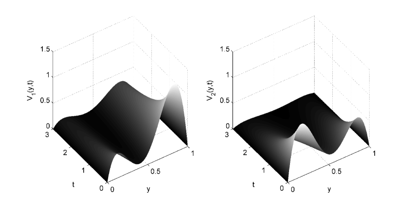
Figure 1: Evolution in time of the approximated solution in the fixed boundary problem for $v_{1}$ (left) and $v_{2}$ ( right).

The picture on the left in Figure 1 illustrates the evolution in time of the obtained solution for $v_{1}$ in the fixed boundary problem, and the picture on the right illustrates the evolution in time of the obtained solution for $v_{2}$. This solution was calculated with approximations of degree two and $h=\delta=10^{-2}$.

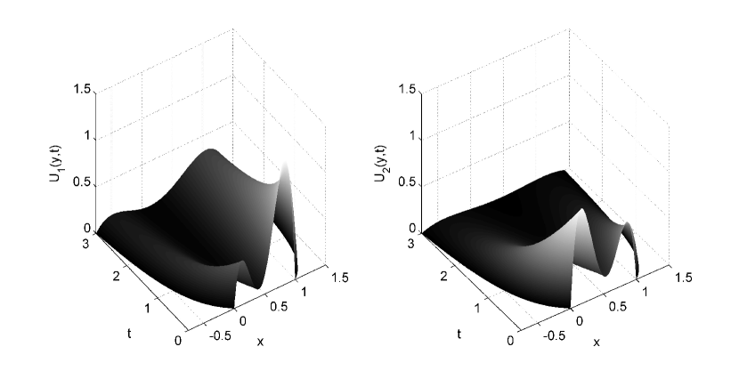
Figure 2: Evolution in time of the approximated solution in the moving boundary problem for $u_{1}$ (left) and $u_{2}$ ( right).

The pictures in Figure 2 represent the obtained solutions in the moving boundary domain, after applying the inverse transformation $\tau^{-1}(y,t)$. In this case $u$ and $v$ could represent the density of two populations of bacteria. We observe that, initially, each population is concentrated mainly in two regions and, as time increases, the two populations decrease and spread out in the domain, as expected.

In order to analyze the convergence rates, this problem was simulated with different combinations of $k$, $h$ and $\delta$ and the error results are represented in Figure 3.

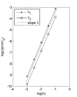
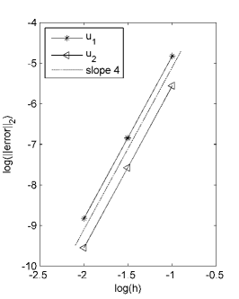
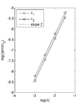
Figure 3: Study of the convergence for $h$ with approximations of degree 2 (left) and 3 (center), and for $\delta$ (right).

The error was calculated in $t=T$ and using the $L_{2}(\alpha(T),\beta(T))$-norm in the space variable. In the picture on the left the logarithms of the errors versus the logarithm of $h$ for the simulations done with $\delta=10^{-4}$ and approximations of degree $2$, are represented. The errors versus the logarithm of $h$ for the simulations done with $\delta=10^{-4}$ and approximations of degree $3$ are represented in the picture in the center. The logarithms of the errors versus the logarithm of $\delta$ for the simulations done with $h=10^{-3}$ and approximations of degree $2$, are represented in the picture on the right. As expected, the pictures are in accordance with the orders of convergence for $h$ and $\delta$, as was proved in Theorem 4.1. In Table 1 we compare the error of the present method with the error of the moving finite element method presented in [20]. Both simulations were done with approximations of degree five and four finite elements. We used $\delta=10^{-4}$ for the present method and $10^{-10}$ for the integrator’s error tolerance in the moving finite element method.

	$\displaystyle\max_{j=1,\dots,np}\{|u_{1}(P_{j},t_{i})-U_{1}^{(i)}(P_{j})|\}$		$\displaystyle\max_{j=1,\dots,np}\{|u_{2}(P_{j},t_{i})-U_{2}^{(i)}(P_{j})|\}$
$t_{i}$	MFEM[20]	present	MFEM[20]	present
$0.001$	7.3025e-08	2.6502e-10	4.2464e-08	6.3606e-10
$0.005$	8.9490e-08	1.0338e-09	5.2037e-08	1.4457e-09
$0.01$	2.7945e-08	1.4645e-09	1.6249e-08	1.8010e-09
$0.02$	1.3320e-08	1.8424e-09	7.7437e-09	2.0228e-09
$0.05$	7.2664e-08	2.0530e-09	4.2203e-08	2.1597e-09
$0.5$	1.9044e-08	1.0564e-09	1.0743e-08	1.0907e-09
$1$	2.1230e-08	5.0614e-10	9.3304e-09	5.5859e-10

Table 1: Comparison of the present method with the moving finite element method in [20]

5.2 Example 2

As a second example, we choose to simulate the second example presented in [20]. This will permit us to compare the present method with an adaptive one. Consider problem (3) with $ne=2$ and $Q_{t}$ defined by

$$\alpha(t)=\sqrt{2/3}-\sqrt[3]{t+(2/3)^{3/2}},\quad\beta(t)=1-\alpha(t),\quad 0\leq t\leq 1.$$

The diffusion coefficients are

$$a_{1}(r,s)=2-\frac{1}{1+s^{2}},\quad a_{2}(r,s)=e^{-r^{2}},$$

and the reaction forces are

$$f_{1}(x,t)=\frac{0.1x}{(1+t)^{4}},\quad f_{2}(x,t)=\frac{e^{-x^{2}}}{(1+t)^{6}}.$$

The initial conditions $u_{10}$ and $u_{20}$ are the natural spline functions of degree three that interpolate the points $\{(0,0),(0.2,1),(0.5,0.5),(1,0)\}$ and $\{(0,0),\linebreak(0.6,0.65),(0.8,1),(1,0)\},$ respectively. The approximate solutions were obtained with four finite elements ($h=0.25$), $\delta=10^{-3}$ and $k=4$. The obtained solutions in the fixed domain are plotted in Figure $4$.

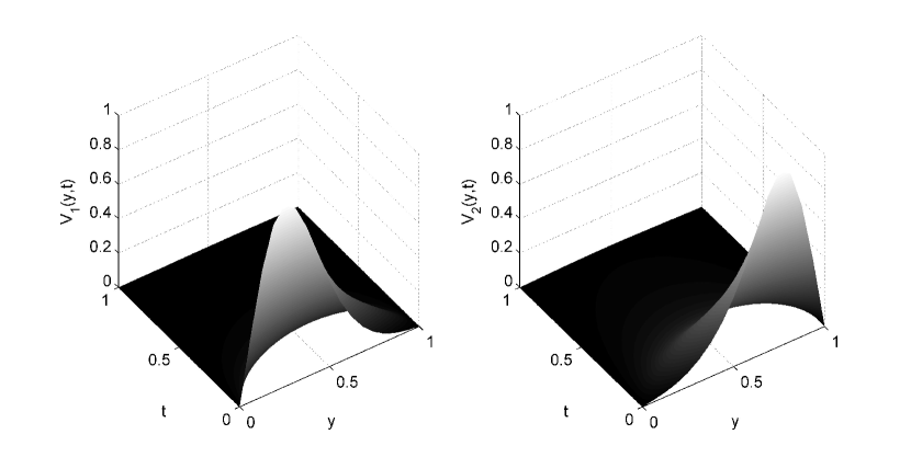
Figure 4: Evolution in time of the approximated solution in the fixed boundary problem for $v_{1}$ (left) and $v_{2}$ ( right).

The pictures in Figure 5 represent the obtained solutions in the moving boundary domain, after applying the inverse transformation $\tau^{-1}(y,t)$. In this example, initially, each population occupies mainly one region opposite from the other population. As the time increases the two populations expands to all the domain and decreases very quickly.

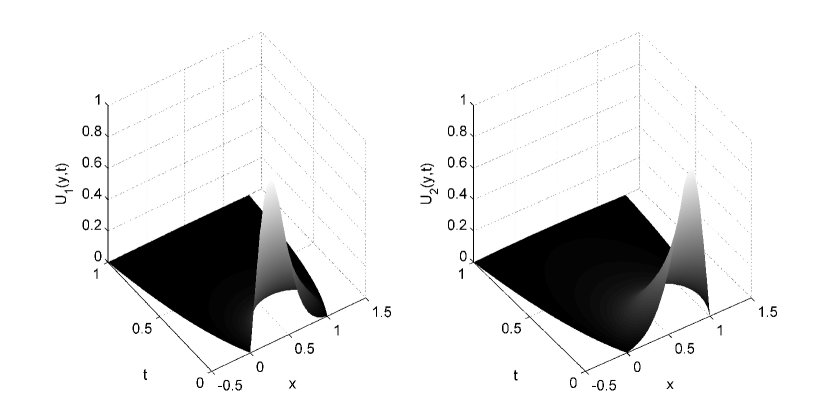
Figure 5: Evolution in time of the approximated solution in the moving boundary problem for $u_{1}$ (left) and $u_{2}$ ( right).

The pictures are similar to those in [20] and the numerical comparisons between the two methods show that the methods are similar. However, due to the fact that in [20] an adaptive mesh was used, initially the difference between the methods is greater in the areas where the solution has a higher slope, but this difference become less significant as time grows.

6 Conclusions

We proved optimal rates of convergence for a linearized Crank-Nicolson-Galerkin finite element method with piecewise polynomial of arbitrary degree basis functions in space when applied to a system of nonlocal parabolic equations. Some numerical experiments were presented, considering different functions $a$, $f$, $\alpha$ and $\beta$. The numerical results are in accordance with the theoretical results and are similar in accuracy to results obtained by other methods.

References

- [1] Azmy S. Ackleh and Lan Ke. Existence-uniqueness and long time behavior for a class of nonlocal nonlinear parabolic evolution equations. Proc. Amer. Math. Soc., 128(12):3483–3492 (electronic), 2000.
-
[2]
Rui M. P. Almeida, José C. M. Duque, Jorge Ferreira, and Rui J. Robalo.
The Crank-Nicolson-Galerkin finite element method for a
nonlocal parabolic equation with moving boundaries.
Available from:
http://ptmat.fc.ul.pt/arquivo/docs/preprints/pdf/2013/Jorge_Ferreira_
Almeida_Duque_preprint_017_2013.pdf, 2013. - [3] Rachid Benabidallah and Jorge Ferreira. On hyperbolic-parabolic equations with nonlinearity of Kirchhoff-Carrier type in domains with moving boundary. Nonlinear Anal., 37(3, Ser. A: Theory Methods):269–287, 1999.
- [4] Mostafa Bendahmane and Mauricio A. Sepúlveda. Convergence of a finite volume scheme for nonlocal reaction-diffusion systems modelling an epidemic disease. Discrete Contin. Dyn. Syst. Ser. B, 11(4):823–853, 2009.
- [5] A. C. Briozzo, M. F. Natale, and D. A. Tarzia. Explicit solutions for a two-phase unidimensional Lamé-Clapeyron-Stefan problem with source terms in both phases. J. Math. Anal. Appl., 329(1):145–162, 2007.
- [6] M. M. Cavalcanti, V. N. Domingos Cavalcanti, J. Ferreira, and R. Benabidallah. On global solvability and asymptotic behaviour of a mixed problem for a nonlinear degenerate Kirchhoff model in moving domains. Bull. Belg. Math. Soc. Simon Stevin, 10(2):179–196, 2003.
- [7] N.-H. Chang and M. Chipot. Nonlinear nonlocal evolution problems. RACSAM. Rev. R. Acad. Cienc. Exactas Fís. Nat. Ser. A Mat., 97(3):423–445, 2003.
- [8] M. Chipot. Elements of nonlinear analysis. Birkhäuser Advanced Texts: Basler Lehrbücher. [Birkhäuser Advanced Texts: Basel Textbooks]. Birkhäuser Verlag, Basel, 2000.
- [9] M. Chipot and B. Lovat. Some remarks on nonlocal elliptic and parabolic problems. In Proceedings of the Second World Congress of Nonlinear Analysts, Part 7 (Athens, 1996), volume 30, pages 4619–4627, 1997.
- [10] M. Chipot and B. Lovat. On the asymptotic behaviour of some nonlocal problems. Positivity, 3(1):65–81, 1999.
- [11] M. Chipot and M. Siegwart. On the asymptotic behaviour of some nonlocal mixed boundary value problems. In Nonlinear analysis and applications: to V. Lakshmikantham on his 80th birthday. Vol. 1, 2, pages 431–449. Kluwer Acad. Publ., Dordrecht, 2003.
- [12] M. Chipot, V. Valente, and G. Vergara Caffarelli. Remarks on a nonlocal problem involving the Dirichlet energy. Rend. Sem. Mat. Univ. Padova, 110:199–220, 2003.
- [13] Michel Chipot and Luc Molinet. Asymptotic behaviour of some nonlocal diffusion problems. Appl. Anal., 80(3-4):279–315, 2001.
- [14] F. J. S. A. Corrêa, Silvano D. B. Menezes, and J. Ferreira. On a class of problems involving a nonlocal operator. Appl. Math. Comput., 147(2):475–489, 2004.
-
[15]
José C. M. Duque, Rui M. P. Almeida, Stanislav N. Antontsev, and Jorge
Ferreira.
The Euler-Galerkin finite element method for a nonlocal coupled
system of reaction-diffusion type.
Available from:
http://ptmat.fc.ul.pt/arquivo/docs/preprints/pdf/2013/Duq_Ant_preprint
_014_2013.pdf, 2013. -
[16]
José C. M. Duque, Rui M. P. Almeida, Stanislav N. Antontsev, and Jorge
Ferreira.
A reaction-diffusion model for the nonlinear coupled system:
existence, uniqueness, long time behavior and localization properties of
solutions.
Available from:
http://ptmat.fc.ul.pt/arquivo/docs/preprints/pdf/2013/preprint_2013_08_
Antontsev.pdf, 2013. - [17] Robert Eymard, Thierry Gallouët, Raphaèle Herbin, and Anthony Michel. Convergence of a finite volume scheme for nonlinear degenerate parabolic equations. Numer. Math., 92(1):41–82, 2002.
- [18] Jorge Ferreira and Nickolai A. Lar′kin. Decay of solutions of nonlinear hyperbolic-parabolic equations in noncylindrical domains. Commun. Appl. Anal., 1(1):75–81, 1997.
- [19] Carlos Alberto Raposo, Mauricio Sepúlveda, Octavio Vera Villagrán, Ducival Carvallo Pereira, and Mauro Lima Santos. Solution and asymptotic behaviour for a nonlocal coupled system of reaction-diffusion. Acta Appl. Math., 102(1):37–56, 2008.
-
[20]
R. J. Robalo, R. M. Almeida, M. C. Coimbra, and J. Ferreira.
Global solvability, exponential decay and mfem approximate solution
of a nonlinear coupled system with moving boundary.
Available from:
http://ptmat.fc.ul.pt/arquivo/docs/preprints/pdf/2013/preprint_015_
CMAF_Jorge_Ferreira.pdf, 2013. -
[21]
R. J. Robalo, R. M. Almeida, M. C. Coimbra, and J. Ferreira.
A reaction-diffusion model for a class of nonlinear parabolic
equations with moving boundaries: existence, uniqueness, exponential decay
and simulation.
Available from:
http://ptmat.fc.ul.pt/arquivo/docs/preprints/pdf/2013/preprint_012_
CMAF_Jorge_Ferreira.pdf, 2013. - [22] M. L. Santos, J. Ferreira, and C. A. Raposo. Existence and uniform decay for a nonlinear beam equation with nonlinearity of Kirchhoff type in domains with moving boundary. Abstr. Appl. Anal., (8):901–919, 2005.
- [23] M. L. Santos, M. P. C. Rocha, and J. Ferreira. On a nonlinear coupled system for the beam equations with memory in noncylindrical domains. Asymptot. Anal., 45(1-2):113–132, 2005.
- [24] Vidar Thomée. Galerkin finite element methods for parabolic problems, volume 25 of Springer Series in Computational Mathematics. Springer-Verlag, Berlin, second edition, 2006.
- [25] S. Zheng and M. Chipot. Asymptotic behavior of solutions to nonlinear parabolic equations with nonlocal terms. Asymptot. Anal., 45(3-4):301–312, 2005.