A Model for Overscreened Kondo Effect in Ultracold Fermi Gas

Abstract

The feasibility of realizing overscreened Kondo effect in ultra-cold Fermi gas of atoms with spin $s\geq\tfrac{3}{2}$ in the presence of a localized magnetic impurity atom is proved realistic. Specifying (as a mere example), to a system of ultra cold ²²Na Fermi gas and a trapped ¹⁹⁷Au impurity, the mechanism of exchange interaction between the Na and Au atoms is elucidated and the exchange constant is found to be positive (antiferromagnetic). The corresponding exchange Hamiltonian is derived, and the Kondo temperature is estimated at the order of $1~{}\mu$K. Within a weak-coupling renormalization group scheme, it is shown that the coupling renormalizes to the non-Fermi liquid fixed point. An observable displaying multi-channel features even in the weak coupling regime is the impurity magnetization: For ${T}\gg{T}_{K}$ it is negative, and then it increases to become positive with decreasing temperature.
 
PACS numbers: 37.10.Jk, 70.10.Hf, 31.15.vn, 33.15.Kr

Introduction: The experimental discovery of Bose-Einstein condensation back in 1996 opened the way to study a myriad of fundamental physical phenomena that were otherwise very difficult to realize (see Ref. bloch for a review). A few years afterward, fabrication and control a cold gas of fermionic atoms has been realized bourdel ; pra04 ; Jin-06 ; pra06 ; NuclPhys07 ; Nature08 ; Li09 ; Nature10 ; Science10 . This revelation opens the way to study the physics of a gas of fermions with (half integer) spin $s\geq\tfrac{3}{2}$. The main axis of the present study relates to the question whether the occurrence of this new state of matter exposes a new facet of Kondo physics.

Single-channel Kondo effect in cold atom physics has been studied in Refs. recati ; gupta ; chen ; ultra-cold-SO3-Kondo ; Christoph . In Ref. Lal10 , the possibility of observing multichannel Kondo effect has been explored for ultra-cold bosonic atoms coupled to an atomic quantum dot, as well as for a system composed of superconducting nano-wires coupled to a Cooper-pair box. Recently, non-Fermi liquid behavior has been predicted for Au monatomic chains containing one Co atom as a magnetic impurity prl13 .

In this work we propose a realization of non-Fermi liquid Kondo effect in cold atoms employing the mechanism leading to over-screening by large spins. The idea is to localize an atom with spin $S$ in a gas of cold fermion atoms of spin $s\geq\frac{3}{2}$ trapped in a combination of harmonic and periodic potentials. If an exchange interaction $J{\bf{s}}\cdot{\bf{S}}$ with $J>0$ exists, the underlying Kondo physics is equivalent to multichannel Kondo effect with large effective number of channels $N_{s}$Kim , that easily satisfies the Nozières-Blandin inequality $N_{s}>2S$, leading to over-screening NB . Possible candidates for fermionic atoms are ²²Na (electronic spin $\frac{1}{2}$, nuclear spin $3$ and total atomic spin $s=\frac{5}{2}$), ⁴⁰K (electronic spin $\frac{1}{2}$, nuclear spin $4$ and total atomic spin $s=\frac{7}{2}$), ⁸⁴Rb or ⁸⁶Rb (electronic spin $\frac{1}{2}$, nuclear spin $2$ and total atomic spin $s=\frac{3}{2}$). Possible candidate for the impurity is ¹⁹⁷Au atom (electronic spin $\frac{1}{2}$, nuclear spin $\frac{3}{2}$ and total atomic spin $S=1$).

Model: Typically, ultra-cold fermi gas is stored in optical dipole traps that rely on the interaction between an induced dipole moment in an atom and an external electric field ${\bf E}({\bf r},t)$. Such oscillating electric (laser) field induces an oscillating dipole moment in the atom. Usually, the trapping potential is formed by three pairs of laser beams of wavelength $\sim 1~{}\mu$m with the use of an acousto-optic modulator, creating a time-averaged optical potential opt-latt-11 ; Nature03 ; arXiv09 ; prb09 ; NaturePhys09 ; Greiner-PhD-03 . This technique gives an anisotropic three dimensional (3D) trap with trapping potential

$$V_{3D}({\bf{R}})=\sum_{i=1,2}V_{1D}^{\parallel}(X_{i})+V_{1D}^{\perp}(X_{3}),$$ (1)

where $X_{1,2,3}$ are Cartesian coordinates of an atom. Each term on the RHS contains a high-frequency wave which forms the oscillating potential and a low-frequency wave which forms the harmonic potential opt-latt-11 ; Nature03 ; arXiv09 ; prb09 ; NaturePhys09 , (see Fig. 1):

$$V_{1D}^{p}(X) = \alpha\lim_{T\to\infty}\frac{1}{T}\int\limits_{0}^{T}dt~{}\big{|}2{\bf{E}}_{f}(X,t)+2{\bf{E}}_{p}(X,t)\big{|}^{2}$$ (2)

$$= V_{f}\sin^{2}(k_{f}X)+V_{p}\big{(}k_{p}X\big{)}^{2},$$

where $\alpha$ is the electric polarizability of atoms, $p=\parallel,\perp$, $V_{f}=2\alpha|{\bf{E}}_{f}|^{2}$ and $V_{p}=2\alpha|{\bf{E}}_{p}|^{2}$ are the lattice potential depths which can be controlled by varying the intensities ${\bf{E}}_{f}$ or ${\bf{E}}_{p}$ of the laser field or the low-frequency waves. The potential parameters are tuned such that

$${V}_{\parallel}k_{\parallel}^{2}\ll{V}_{\perp}k_{\perp}^{2}\ll{V}_{f}k_{f}^{2}.$$ (3)

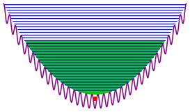
Figure 1: Filling of the energy levels in the potential well $V_{1D}^{\parallel}(X)$ (2) by fermionic atoms. The filled area denotes the occupied energy levels (blue lines), whereas the energy levels in the unfilled area are unoccupied. The red circle denotes the impurity. The purple curve denotes $V_{1D}^{\parallel}(X)$.

To be concrete, we henceforth consider fermionic ²²Na atoms (spin $\tfrac{5}{2}$) and ¹⁹⁷Au impurities (spin $S=1$). The potential well is filled with ²²Na atoms and with sparsely distributed ¹⁹⁷Au atoms. The shallow well $V_{s}$ should be deep enough to trap the heavy Au atom but it cannot trap the Na atoms. As a result, we get an atomic Fermi gas with a low concentration of magnetic impurities.

Atomic Quantum States in the Potential Well:
We consider a neutral atom (nucleus plus core) as a positively charged rigid ion (with filled shell) and one electron on the outer orbital (i.e., 3$s$ orbital in the Na atom or 6$s$ orbital in the Au atom). The positions of the ion and the outer electron are respectively specified by vectors ${\bf{R}}$ and ${\bf{r}}$ [Fig. 1 in the supplementary materials (SM)]. In the adiabatic approximation (which is natural in atomic physics), the wave function of the atom is a product of the corresponding wave functions $\Psi({\bf{R}})$ and $\psi({\bf{r}})$ describing the stationary states of the ion and the outer electron. In order to find the wave functions and energies of the ²²Na and ¹⁹⁷Au ions in the anisotropic 3D potential well, we need to solve the following Schrödinger equation for $\Psi({\bf{R}})=\Psi^{\rm{Au,Na}}({\bf{R}})$,

$$-\frac{\hbar^{2}}{2M}~{}\frac{\partial^{2}\Psi({\bf{R}})}{\partial{\bf{R}}^{2}}+V_{3D}({\bf{R}})\Psi({\bf{R}})=\varepsilon\Psi({\bf{R}}).$$ (4)

Consider first $\Psi^{\rm{Au}}({\bf{R}})$. When the corresponding energy level $\varepsilon_{\rm{imp}}$ is deep enough, the wave function of the bound state near the potential minimum at ${\bf{R}}={\bf{0}}$ can be approximated within the harmonic potential picture as,

$$\Psi^{\rm{Au}}({\bf{R}}) = \frac{1}{\big{(}\pi a_{f}^{2}\big{)}^{\frac{3}{2}}}~{}\exp\bigg{(}-\frac{R^{2}}{2a_{f}^{2}}\bigg{)},$$ (5)

where

$$k_{f}a_{f}=\sqrt{\frac{\hbar\omega_{f}}{V_{f}}},\ \ \ \omega_{f}=\sqrt{\frac{2V_{f}k_{f}^{2}}{M_{\rm{Au}}}},\ \ \ \varepsilon_{\rm{imp}}=\frac{3\hbar\omega_{f}}{2}.$$

Second, consider the wave function of the (much lighter) ²²Na ions, for which the shallow potential wells are not deep enough to form bound states. For studying the Kondo effect we need to focus on quantum states at energies $\varepsilon$ within the deep well close to $\epsilon_{F}$, that is, $\varepsilon\gg{V_{f}}$. In that case we can neglect the “fast” potential relief $V_{f}\sin^{2}(k_{f}x)$, and the solution of Eq. (4) becomes,

$$\Psi_{\nu m\ell}^{\rm{Na}}({\bf{R}}) = \Phi_{\nu m}(R)~{}F_{\ell}(Z)~{}e^{im\phi},$$ (6a)

where $$R \phi Z \rho\equiv R/a_{\parallel} \Phi_{\nu m}(R)$$, and are cylindrical coordinates. Denoting , the radial wave function is,

$$\Phi_{\nu m}(R)=\frac{1}{a_{\parallel}\sqrt{\pi}}~{}\sqrt{\frac{\nu!}{(\nu+|m|)!}}\rho^{|m|}L_{\nu}^{(|m|)}\big{(}\rho^{2}\big{)}e^{\mbox{-}\frac{\rho^{2}}{2}},$$ (6b)

where $$L_{\nu}^{(|m|)} \nu=0,1,2,\ldots m=0,\pm 1,\pm 2,\ldots$$ is the generalized Laguerre polynomial, and , and

$$k_{\parallel}a_{\parallel}=\sqrt{\frac{\hbar\omega_{\parallel}}{V_{\parallel}}},\ \ \ \ \ \omega_{\parallel}=\sqrt{\frac{2V_{\parallel}k_{\parallel}^{2}}{M_{\rm{Na}}}}.$$ (6c)

Denoting $$\zeta\equiv Z/a_{\perp} Z$$ the motion along is described by

$$F_{\ell}(Z) = \frac{1}{\big{(}\pi a_{\perp}^{2}\big{)}^{\frac{1}{4}}}\frac{1}{\sqrt{2^{\ell}~{}\ell!}}H_{\ell}(\zeta)e^{-\zeta^{2}/2},$$ (6d)

where $$H_{\ell} \ell \ell=0,1,2,\ldots$$ is the Hermite polynomial, is the harmonic quantum number, .

$$k_{\perp}a_{\perp}=\sqrt{\frac{\hbar\omega_{\perp}}{V_{\perp}}},\ \ \ \ \ \omega_{\perp}=\sqrt{\frac{2V_{\perp}k_{\perp}^{2}}{M_{\rm{Na}}}}.$$ (6e)

The corresponding energy levels depend on two quantum number, $n=2\nu+|m|$ and $\ell$,

$$\varepsilon_{n\ell}=\hbar\omega_{\parallel}\Big{(}n+1\Big{)}+\hbar\omega_{\perp}\Big{(}\ell+\frac{1}{2}\Big{)}.$$ (7)

When $\omega_{\parallel}$ and $\omega_{\perp}$ are incommensurate, the degeneracy of the level $(n,\ell)$ is $(n+1)(2s+1)$. The inequalities (3) imply $\omega_{\parallel}\ll\omega_{\perp}\ll\omega_{f}$. Restricting the Fermi energy $\epsilon_{F}$ as, $\frac{\hbar\omega_{\perp}}{2}<\epsilon_{F}<\frac{3\hbar\omega_{\perp}}{2}$, the quantum states with $\ell>0$ are frozen at $T\ll\hbar\omega_{\perp}$, hence the Fermi gas is virtually 2D.

The potential well is filled by ²²Na atoms (fermions) and one impurity atom ¹⁹⁷Au. The latter occupies the lowest-energy level (A Model for Overscreened Kondo Effect in Ultracold Fermi Gas) of the potential well and its wave function is well concentrated around the point ${\bf{R}}={\bf{0}}$. Hence, regarding it as a localized impurity is justified.
Na-Au exchange interaction: When the distance between a ²²Na atom and the ¹⁹⁷Au impurity is of the order of $R_{0}$ (the atomic size), there is an exchange interaction between their open electronic $s$ shells Andreev73 . It includes a direct exchange term of strength $J_{d}$ (due to antisymmetrization of the electronic wave functions where electrons do not hop between atoms), and an indirect exchange term of strength $J_{p}$ (due to contribution from polar states, where electrons can hope between atoms). Unlike the case of hydrogen molecule where the direct part dominates, here both of them should be considered since their orders of magnitude are found to be comparable. Evaluating the exchange interaction between Na and Au atoms involves four wave functions: Two of them, $\Psi^{\rm{Au}}({\bf{R}})$ [Eq. (5)] and $\Psi^{\rm{Na}}_{{\nu}{m}{0}}({\bf{R}})$ [Eq. (6a)] pertain to the corresponding atoms as being structureless particles in the optical potential (2). The other two $\psi_{3}^{\rm{Na}}({\bf{r}})$ and $\psi_{6}^{\rm{Au}}({\bf{r}})$ pertain to electronic wave functions of the 3s orbital in Na and 6s orbital in Au,

$$J_{\nu\nu^{\prime},m}=-\frac{2}{(2s+1)(2S+1)}~{}\int\limits_{R_{12}>R_{0}}d^{3}{\mathbf{R}}_{1}d^{3}{\mathbf{R}}_{2}~{}V(R_{12})$$

$$\times\Big{|}\Psi^{\mathrm{Au}}({\mathbf{R}}_{1})\Big{|}^{2}\Big{(}\Psi^{\mathrm{Na}}_{\nu m0}({\mathbf{R}}_{2})\Big{)}^{*}\Psi^{\mathrm{Na}}_{\nu^{\prime}m0}({\mathbf{R}}_{2}),~{}~{}~{}~{}~{}~{}~{}~{}$$ (8)

where ${\mathbf{R}}_{1}$ or ${\mathbf{R}}_{2}$ is the position of the ion of Au or Na, $R_{12}=|{\mathbf{R}}_{1}-{\mathbf{R}}_{2}|$. We assume here that $R_{12}>R_{0}$, since Coulomb repulsion between the electron clouds of the Na and Au atoms prevents the atoms from approaching closer than ${R}_{0}\approx{r}_{\mathrm{Na}}+{r}_{\mathrm{Au}}$ (that is approximated by the sum of the corresponding atomic radii). $V(R)=V_{\mathrm{d}}(R)+\frac{W_{\mathrm{p}}^{2}(R)}{U}$, where $V_{\mathrm{d}}(R)$ is a direct exchange interaction, $W_{\mathrm{p}}(R)$ is the hybridization term and $U$ is a Coulomb blockade. Explicitly they are (see Ref. Davydov-QM and the SM for details),

$$V_{\mathrm{d}}(R_{12}) = \int d^{3}{\bf{r}}_{1}d^{3}{\bf{r}}_{2}~{}\psi_{6}^{\rm{Au}}({\mathbf{r}}_{1}-{\mathbf{R}}_{1})\psi_{3}^{\rm{Na}}({\mathbf{r}}_{2}-{\mathbf{R}}_{2})$$

$$\times\psi_{3}^{\rm{Na}}({\mathbf{r}}_{1}-{\mathbf{R}}_{2})\psi_{6}^{\rm{Au}}({\mathbf{r}}_{2}-{\mathbf{R}}_{1})$$

$$\times\bigg{\{}\frac{e^{2}}{{r}_{12}}+V_{12}(R_{12})+\sum_{i=1}^{2}V_{i}(|{\mathbf{r}}_{i}-{\bf{R}}_{i}|)\bigg{\}},$$

$$W_{\rm{p}}(R_{12}) = \frac{1}{2}\int{d^{3}{\bf{r}}}~{}\sum_{i=1}^{2}V_{i}(|{\bf{r}}-{\bf{R}}_{i}|)$$

$$\times\psi^{\rm{Au}}_{6}({\mathbf{r}}-{\mathbf{R}}_{1})\psi^{\rm{Na}}_{3}({\mathbf{r}}-{\mathbf{R}}_{2}),$$

$$\frac{1}{U} = \frac{1}{U_{\rm{Na}}+\varepsilon_{\rm{Na}}-\varepsilon_{\rm{Au}}}+\frac{1}{U_{\rm{Au}}+\varepsilon_{\rm{Au}}-\varepsilon_{\rm{Na}}}.$$

Here ${\bf{r}}_{1}$ or ${\bf{r}}_{2}$ is the position of electron and ${r}_{12}=|{\bf{r}}_{1}-{\bf{r}}_{2}|$. $V_{1}(r)$ or $V_{2}(r)$ describes the electron-ion interaction for Au or Na, and $V_{12}(R)$ is the interaction between ions. $\varepsilon_{\rm{Na}}=-5.14$ eV and $\varepsilon_{\rm{Au}}=-9.23$ eV are single-electron energies of the sodium and gold atoms, $U_{\rm{Na}}=5.69$ eV and $U_{\rm{Au}}=11.54$ eV are the Coulomb interaction preventing two-electron occupation of the outer orbitals of atoms.

The electronic wave functions decrease rapidly when the distance between the atoms exceeds the atomic radius, so that the exchange interaction may be approximated by a point-like interaction. Moreover, the wave function $\Psi^{\rm{Au}}({\bf{R}})$, Eq.(5), has its maximum at ${\bf{R}}={\bf{0}}$ and it vanishes for ${R}\gg{a_{f}}$. The wave function $\Psi^{\rm{Na}}_{{\nu}{m}{0}}({\bf{R}})$, Eq.(6a), varies slowly on the distance scale of $a_{f}$. Then $|\Psi^{\rm{Au}}({\bf{R}})|^{2}$ can be approximated by the delta-function. Within this approximation, we get the following estimate of the exchange constant, $J_{\nu\nu^{\prime},m}=J\delta_{m0}$, where

$$J = \frac{1}{(2s+1)(2S+1)}~{}\frac{\hbar^{2}(u_{\mathrm{d}}+u_{\mathrm{p}})}{\sqrt{\pi}~{}M_{\mathrm{Na}}~{}a_{\parallel}^{2}~{}a_{\perp}},$$ (9)

where $u_{\mathrm{d}}$ and $u_{\mathrm{p}}$ are scattering lengths of the direct and indirect exchange interactions. Expressions for $u_{\mathrm{d}}$ and $u_{\mathrm{p}}$ in terms of the potentials of the direct and indirect exchanges as well as the explicit form for the exchange potentials are standard and can be found in textbooks [see e.g. Refs. Sitenko ; Landau-Lifshitz-3 ; Davydov-QM and Eqs. (12) and (13) in the Supplementary Material]. Numerical estimations yields $u_{\mathrm{d}}\approx 1.24~{}\mu$m and $u_{\mathrm{p}}=1.49~{}\mu$m. In Refs. Landau-Lifshitz-3 ; Davydov-QM it was shown that $J_{\mathrm{d}}>0$. Since $J_{\mathrm{p}}>0$ (always), the total exchange interaction is anti-ferromagnetic.

Kondo Hamiltonian and the Kondo temperature: Eq. (9) indicates that, due to centrifugal barrier, only atoms in s-states interact with the impurity. Omitting the quantum numbers $\ell=m=0$ for brevity, we write the Hamiltonian of the system as $H=H_{0}+H_{K}$, where

$$H_{0}=\sum_{\nu\mu}\varepsilon_{2\nu}~{}c_{\nu\mu}^{{\dagger}}c_{\nu\mu},\ \ \ \ \ H_{K}=J~{}\big{(}{\bf{S}}\cdot{\bf{s}}\big{)}.$$ (10)

Here $c_{\nu\mu}$ or $c_{\nu\mu}^{{\dagger}}$ is the annihilation or creation operator of a sodium atom in the state with the principal quantum number $2\nu$ and $\ell=m=0$, $\varepsilon_{2\nu}\equiv\varepsilon_{2\nu 0}$ is given by Eq. (7), $\mu$ denotes atomic spin projection, ${\bf{S}}$ is the impurity spin and ${\bf{s}}=\sum_{\nu\nu^{\prime},\mu\mu^{\prime}}c_{\nu\mu}^{{\dagger}}{\mathbf{t}}_{\mu\mu^{\prime}}c_{\nu^{\prime}\mu^{\prime}},$ where $\hat{\mathbf{t}}$ is the vector of the spin-$s$ matrices.

The density of states (DOS) for the Hamiltonian $H_{0}$ is

$$\rho(\epsilon) = \sum_{\nu=0}^{\infty}\delta(\epsilon-\varepsilon_{2\nu})=\frac{\vartheta(\epsilon)}{2\hbar\omega_{\parallel}},$$ (11)

where $\vartheta(\epsilon)$ is the Heaviside theta function.

Within poor-man scaling formalism for multy-channel Kondo effect, the dimensionless coupling $j=J\rho(\epsilon_{F})$ satisfies the following scaling equation NB ,

$$\frac{\partial{j}(D)}{\partial\ln{D}} = -j^{2}(D)+N_{s}j^{3}(D),$$ (12)

with $N_{s}=\frac{2}{3}s(s+1)(2s+1)$ being an effective number of channels Kim . Initially, the bandwidth is ${D_{0}}\geq{D}\gg{T}$ and the initial value of $j(D)$ is,

$$j(D_{0})\equiv j_{0}=\frac{1}{(2s+1)(2S+1)}~{}\frac{u_{d}+u_{p}}{2\sqrt{\pi}~{}a_{\perp}},$$

where $a_{\perp}$ is given by Eq.(6e).

The solution of Eq.(12) is,

$$\ln\bigg{(}\frac{D_{0}}{D}\bigg{)}=\frac{1}{j_{0}}-\frac{1}{j}+N_{s}\ln\frac{j(1-N_{s}j_{0})}{j_{0}(1-N_{s}j)}.$$ (13)

When $D\to 0$, $j(D)$ renormalizes to the weak coupling fixed point $j^{*}=1/N_{s}$. When $|j(D)-j^{*}|\ll{j^{*}}$, the solution for $j(D)$ reduces asymptotically to,

$$\frac{j^{*}-j(D)}{j^{*}}=\frac{j^{*}-j_{0}}{j_{0}}~{}\bigg{(}\frac{D~{}T^{*}}{D_{0}T_{K}}\bigg{)}^{j^{*}},$$ (14)

see Ref. Hewson-book , where

$$T^{*}=D_{0}\exp\bigg{(}-\frac{1}{j^{*}}\bigg{)},\ \ \ T_{K}=D_{0}\exp\bigg{(}-\frac{1}{j_{0}}\bigg{)}.$$ (15)

The scaling equation (12) accounts for the evolution of $j(D)$ only when the atomic spin $s\geq\frac{3}{2}$.

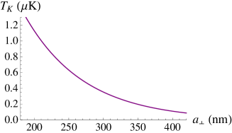
Figure 2: $T_{K}$, Eq.  (15) as a function of $a_{\perp}$ for $D_{0}\approx{V_{f}}=1$ neV.

The Kondo temperature (15) as a function of $a_{\perp}$ is shown in Fig. 2 for $D_{0}\approx{V_{f}}=1$ neV. It is seen that $T_{K}$ changes from $100$ nK to $1.1~{}\mu$K for $a_{\perp}=200\div 400$ nm, so that the ratio $\frac{T_{K}}{D_{0}}\approx 0.01\div 0.1$ is really small, whereas ${T}\sim{T}_{K}$ may be experimentally reachable. Indeed, more than a decade ago, ⁴⁰P atoms were cooled to a temperature of 50 nK Nature03 , later the ¹³³Cs atoms were cooled to temperature 40 nK NaturePhys09 ; arXiv09 .

Impurity magnetization: Having elaborated upon the theory, we are now in a position to carry out perturbation calculations of experimental observables. It is sometimes argued that the interesting physics in the over-screens Kondo effect is exposed only in the strong coupling regime. Here we show that peculiar behaviour emerges also in the weak coupling regime. The reason is that the weak coupling fixed point $j^{*}$ is small, and in most cases, the initial value of $j(D_{0})>j^{*}$. As the temperature $T$ is reduced toward $T_{K}$, $j(D)$ decreases toward $j^{*}$ and as a results, some physical observables display an unusual dependence on temperature. Consider for example the impurity magnetization ${\bf{M}}_{\rm{imp}}(T)=M_{\rm{imp}}(T)\hat{\bf B}$ in response to an external magnetic field ${\bf B}$. Experimentally it requires immersing a small concentration $n_{i}$ of impurity atoms in the gas of fermionic atoms. Within third order perturbation theory, we have,

$$M_{\rm{imp}}=\frac{B\chi_{0}T^{*}}{T}~{}\Bigg{\{}\frac{S}{S+1}-\frac{SN_{s}}{s+1}~{}\bigg{[}j+$$

$$+j^{2}\Big{(}1-jN_{s}\Big{)}\ln\bigg{(}\frac{D_{0}}{T}\bigg{)}\bigg{]}\Bigg{\}},\ \ \chi_{0}=\frac{g_{e}^{2}\mu_{B}^{2}n_{i}}{12T^{*}},$$ (16)

where $g_{e}\approx 2$ is the electronic spin g-factor and $\mu_{B}$ is the Bohr magneton.

Due to the logarithmic terms, which, strictly speaking, are not small either, the terms proportional to $j^{2}$ and $j^{3}$ are not small as compared with $j$. Hence, expansion up to the third order in $j$ is inadequate. Instead, we derive an expression for the impurity related magnetization in the leading logarithmic approximation using the RG equations (12). The condition imposing invariance of the magnetization under “poor man’s scaling” transformation has the form Hewson-book ,

$$\frac{\partial}{\partial D}\bigg{[}j+j^{2}\Big{(}1-jN_{s}\Big{)}\ln\bigg{(}\frac{D}{T}\bigg{)}\bigg{]}=0.$$ (17)

Eq. (17) yields the scaling equation (12). The renormalization procedure should proceed until the bandwidth $D$ is reduced to the temperature $T$. The expression for the impurity related magnetization then becomes,

$$M_{\rm{imp}}=\frac{B\chi_{0}T^{*}}{T}X(T),\ \ X(T)=\frac{S}{S+1}-\frac{S}{s+1}~{}\frac{j(T)}{j^{*}}.$$ (18)

The function $X(T)$ consists of two terms. The first one describes the Zeeman interaction of the impurity with the external magnetic field and results in the Curie’s law. The second one corresponds to the exchange interaction of the impurity with atoms (the atomic magnetization is parallel to the external magnetic field). When the exchange interaction of the impurity is stronger than the Zeeman interaction, the function $X(T)$ is negative and the impurity magnetization is anti-parallel to the external magnetic field. This occurs when $j(T)$ exceeds some critical value, $j_{c}=j^{*}\frac{s+1}{S+1}$.

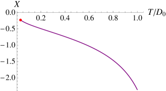
Figure 3: The function $X(T)$, Eq. (18), as a function of temperature for $j_{0}=0.286$. The red dot corresponds to $T=T_{K}$.

Fig. 3 illustrates $X(T)$ for $j_{0}=0.286$. It is seen that at high temperatures when $j(T)>j_{c}$, $X$ is negative, and the impurity magnetization is anti-parallel to the external magnetic field. With reducing the temperature, the effective coupling $j(T)$ reduces as well. At temperature $T_{c}$ satisfying $j(T_{c})=j_{c}$, $X(T)$ changes sign from negative for $T>T_{c}$ to positive for $T<T_{c}$. For the given parameter values, $T_{c}\ll T_{K}$ and, strictly speaking, cannot be estimated within the framework of the poor man’s scaling technique.

Conclusions: The non-Fermi liquid Kondo effect can be accessed within the realm of cold atom physics. Exchange Hamiltonian is derived and scaling equations are solved for an ultra-cold gas of alkali atoms [such as ²²Na] with ¹⁹⁷Au impurity. The dimensionless coupling $j$ is not extremely small even though the coupling $J$, Eq. (9), is small. Such over-screened Kondo effect by fermions of large spin may be exposed even in the weak coupling regime through the temperature dependence of the impurity magnetization.
 
Acknowledgement: We would like to thank N. Andrei, O. Parcollet, Y. Castin and C. Salomon for important discussions and numerous suggestions during the early stages of this research. This work is supported by grant 400/2012 of the Israeli Science Foundations (ISF).

Appendix A Supplementary Material

Here we expand upon the derivation of exchange constants between ²²Na and ¹⁹⁷Au that are required to arrive at the Kondo Hamiltonian (10) of the main text. First we elucidate the direct exchange and then the indirect one. As it turn out, both of them are positive for realistic inter-atomic distance $R_{12}$ and they are of the same order of magnitude.

A.1 Direct Exchange Contribution

Let atoms of gold and sodium be at positions ${\mathbf{R}}_{1}$ and ${\mathbf{R}}_{2}$, with the distance between them $R_{12}=|{\mathbf{R}}_{1}-{\mathbf{R}}_{2}|$. Then the direct exchange interaction $V_{\mathrm{d}}(R_{12})$ between the atoms is (see Ref.[29]),

$$V_{\rm{d}}(R_{12}) = \int d^{3}{\bf{r}}_{1}d^{3}{\bf{r}}_{2}~{}\psi_{6}^{\rm{Au}}({\mathbf{r}}_{1}-{\mathbf{R}}_{1})\psi_{3}^{\rm{Na}}({\mathbf{r}}_{2}-{\mathbf{R}}_{2})\psi_{3}^{\rm{Na}}({\mathbf{r}}_{1}-{\mathbf{R}}_{2})\psi_{6}^{\rm{Au}}({\mathbf{r}}_{2}-{\mathbf{R}}_{1})\times$$ (19)

$$\times\bigg{\{}\frac{e^{2}}{{r}_{12}}+V_{12}(R_{12})+V_{1}(|{\mathbf{r}}_{1}-{\bf{R}}_{1}|)+V_{2}(|{\mathbf{r}}_{2}-{\mathbf{R}}_{2}|)\bigg{\}}.$$

Here ${\bf{r}}_{1}$ or ${\bf{r}}_{2}$ is the position of electron, see Fig. 4 and ${r}_{12}=|{\bf{r}}_{1}-{\bf{r}}_{2}|$. We assume here that $R_{12}>R_{0}$, since Coulomb repulsion between the electron clouds of the Na and Au atoms prevents the atoms from approaching closer than ${R}_{0}\approx{r}_{\mathrm{Na}}+{r}_{\mathrm{Au}}$ (that is approximated by the sum of the corresponding atomic radii). In Eq. (19), $V_{1}(r)$ or $V_{2}(r)$ describes the electron-ion interaction for Au or Na, and $V_{12}(R)$ is the interaction between ions. When the inter-atomic distance exceeds $R_{0}$, we can write,

$$V_{1}(r)\approx V_{2}(r)\approx-\frac{e^{2}}{r},\ \ \ \ \ V_{12}(R)\approx\frac{e^{2}}{R}.$$

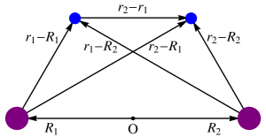
Figure 4: Two atoms. Position of electron of the first or second atom is ${\bf{r}}_{1}$ or ${\bf{r}}_{2}$, the radius vector between the nuclei is ${\bf{R}}$.

The function $V_{\mathrm{d}}(R)$ calculated numerically for the hydrogen-like electronic wave functions $\psi_{3}^{\rm{Na}}({\bf{r}})$ and $\psi_{6}^{\rm{Au}}({\bf{r}})$ is shown in Fig. 5, dashed purple curve. It is negative for any $R>R_{0}$ [where $R_{0}\approx 3.3$ Å for the atoms of sodium and gold], so that the exchange interaction is anti-ferromagnetic.

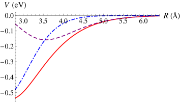
Figure 5: Direct exchange interaction $V_{\mathrm{d}}(R)$ [Eq. (19), dashed purple curve], indirect exchange interaction $V_{\mathrm{p}}(R)$ [Eq. (20), dashed and dotted blue curve] and the total exchange interaction $V(R)$ [Eq. (23), solid red curve] as functions of the distances $R$ between the nuclei.

A.2 Indirect Exchange Contribution

Indirect exchange interaction between the atoms Na and Au separated by distance $R_{12}$ is

$$V_{\mathrm{p}}(R_{12}) = -\frac{W_{\rm{p}}^{2}(R_{12})}{U},$$ (20)

where

$$\frac{1}{U}~{}=~{}\frac{1}{U_{\rm{Na}}+\varepsilon_{\rm{Na}}-\varepsilon_{\rm{Au}}}+\frac{1}{U_{\rm{Au}}+\varepsilon_{\rm{Au}}-\varepsilon_{\rm{Na}}},$$

$\varepsilon_{\rm{Na}}=-5.14$ eV and $\varepsilon_{\rm{Au}}=-9.23$ eV are single-electron energies of the sodium and gold atoms, $U_{\rm{Na}}=5.69$ eV and $U_{\rm{Au}}=11.54$ eV are the Coulomb interaction preventing two-electron occupation of the outer orbitals of atoms.

The hybridization term $W_{\mathrm{p}}(R)$ in Eq. (20) is given explicitly as,

$$W_{\rm{p}}(R) = \frac{1}{2}\int{d^{3}{\bf{r}}}~{}\Big{\{}V_{1}(|{\bf{r}}|)+V_{2}(|{\bf{r}}-{\bf{R}}|)\Big{\}}~{}\psi^{\rm{Au}}_{6}({\bf{r}})\psi^{\rm{Na}}_{3}({\bf{r}}-{\bf{R}}).$$ (21)

The function $V_{\mathrm{p}}(R)$ calculated numerically for the hydrogen-like electronic wave functions $\psi_{3}^{\rm{Na}}({\bf{r}})$ and $\psi_{6}^{\rm{Au}}({\bf{r}})$ is shown in Fig. 5, dashed and dotted blue curve. It is is always negative, so that the indirect exchange interaction is anti-ferromagnetic.

A.3 Projecting the Exchange Interaction onto the States with a Given Total Spin

The exchange interaction Hamiltonian can be written as,

$$H_{\mathrm{ex}}(R_{12}) = -2V(R_{12})~{}\big{(}{\mathbf{s}}_{1}\cdot{\mathbf{s}}_{2}\big{)},$$ (22)

where

$$V(R) = V_{\mathrm{d}}(R)+V_{\mathrm{p}}(R).$$ (23)

$V(R)$ calculated numerically for the hydrogen-like electronic wave functions $\psi_{3}^{\rm{Na}}({\bf{r}})$ and $\psi_{6}^{\rm{Au}}({\bf{r}})$ is shown in Fig. 5, solid red curve. It is seen that $V(R)<0$, so that the coupling is anti-ferromagnetic. ${\mathbf{s}}_{1}$ or ${\mathbf{s}}_{2}$ is spin operator for the outer s-electron of the gold or sodium atom,

$${\mathbf{s}}_{j}=\frac{1}{2}\sum_{\sigma\sigma^{\prime}}d_{j\sigma}^{{\dagger}}{\bm{\tau}}_{\sigma\sigma^{\prime}}d_{j\sigma^{\prime}},$$

where $\hat{\bm{\tau}}$ is a vector of the Pauli matrices, $d_{j\sigma}$ or $d_{j\sigma}^{{\dagger}}$ is the annihilation or creation operator of electron with spin $\sigma=\uparrow,\downarrow$.

Atom of ¹⁹⁷Au has the nuclear spin $s_{\rm{Au}}=\frac{3}{2}$, so the quantum state of an atom, $|\sigma,\mu\rangle$, is described by projection of the nuclear spin $\mu$ on the axis $z$ and electronic spin $\sigma$. Anti-ferromagnetic hyperfine interaction couples nuclear and electron spins in total atomic spin $s=s_{\mathrm{Au}}-\frac{1}{2}=1$. The wave function $|S,m\rangle$ of the state with the total spin $S$ and the projection of the spin $m$ on the axis $z$ is,

$$\big{|}S,m\big{\rangle} = \sqrt{\frac{S+1-m}{2(S+1)}}~{}\bigg{|}\uparrow,m-\frac{1}{2}\bigg{\rangle}-\sqrt{\frac{S+1+m}{2(S+1)}}~{}\bigg{|}\downarrow,m+\frac{1}{2}\bigg{\rangle}.$$ (24)

Projecting out the electronic spin operator ${\mathbf{s}}_{1}$ onto the quantum states (24), we get

$${\mathbf{s}}_{1} \to \sum_{mm^{\prime}}\big{|}S,m\big{\rangle}\big{\langle}S,m\big{|}{\mathbf{s}}_{1}\big{|}S,m^{\prime}\big{\rangle}\big{\langle}S,m^{\prime}\big{|}~{}=~{}\frac{\mathbf{S}}{2S+1},\ \ \ \ \ {\mathbf{S}}~{}=~{}\sum_{mm^{\prime}}{\mathbf{T}}_{mm^{\prime}}~{}X^{mm^{\prime}}_{\mathrm{Au}},$$ (25)

where $\hat{\mathbf{T}}$ is a vector of the spin-$s$ matrices,

$$X^{mm^{\prime}}_{\mathrm{Au}} = \big{|}S,m\big{\rangle}\big{\langle}S,m^{\prime}\big{|}.$$

Similarly, the nuclear spin of ²²Na is $s_{\mathrm{Na}}=3$, the total atomic spin is $s=3-\frac{1}{2}=\frac{5}{2}$. The wave function $|s,m\rangle$ of the quantum state with the total spin $s$ and projection $m$ of the spin on the $z$-axis is given by Eq.(24) with ${S}\to{s}$. Then projecting out the electronic spin operator ${\mathbf{s}}_{2}$ onto the quantum states (24), we get

$${\mathbf{s}}_{2} \to \sum_{mm^{\prime}}\big{|}s,m\big{\rangle}\big{\langle}s,m\big{|}{\mathbf{s}}_{1}\big{|}s,m^{\prime}\big{\rangle}\big{\langle}s,m^{\prime}\big{|}~{}=~{}\frac{\mathbf{s}}{2s+1},\ \ \ \ \ {\mathbf{s}}~{}=~{}\sum_{mm^{\prime}}{\mathbf{t}}_{mm^{\prime}}~{}X^{mm^{\prime}}_{\mathrm{Na}},$$ (26)

where $\hat{\mathbf{t}}$ is a vector of the spin-$s$ matrices,

$$X^{mm^{\prime}}_{\mathrm{Na}} = \big{|}s,m\big{\rangle}\big{\langle}s,m^{\prime}\big{|}.$$

Finally, the exchange Hamiltonian (22) takes the form,

$$H_{\mathrm{ex}}(R_{12}) = -\frac{2V(R_{12})}{(2s+1)(2S+1)}~{}\big{(}{\mathbf{s}}\cdot{\mathbf{S}}\big{)}.$$ (27)

A.4 Derivation of the Coupling $J$

Atoms of sodium and gold place in the external potential given by Eq. (1) of the main text. The wave function $\Psi^{\mathrm{Au}}({\mathbf{R}})$ of the atom of gold is given by Eq. (5) of the main text, whereas the wave functions $\Psi^{\mathrm{Na}}_{\nu m0}({\mathbf{R}})$ of the atoms of sodium are given by Eq.(6a) of the main text. Then the coupling is,

$$J_{\nu\nu^{\prime},m}=-\frac{2}{(2s+1)(2S+1)}~{}\int\limits_{R_{12}\geq{R_{0}}}d^{3}{\bf{R}}_{1}d^{3}{\bf{R}}_{2}~{}V(R_{12})~{}\Big{|}\Psi^{\rm{Au}}\big{(}{\bf{R}}_{1}\big{)}\Big{|}^{2}~{}\Big{(}\Psi^{\rm{Na}}_{\nu m0}\big{(}{\bf{R}}_{2}\big{)}\Big{)}^{*}~{}\Psi^{\rm{Na}}_{\nu^{\prime}m0}\big{(}{\bf{R}}_{2}\big{)},$$ (28)

where $V(R)$ is given by Eq.(23). The sign of $J_{\nu\nu^{\prime},m}$ is chosen in such a way that positive coupling strength corresponds to anti-ferromagnetic interaction. The integration on the RHS of Eq.(28) is restricted by the condition $R_{12}>R_{0}$, since Coulomb repulsion between the electron clouds of the Na and Au atoms prevents the atoms from approaching closer than $R_{0}$.

The function $V(R)$ is negative for any $R>R_{0}$ (see Fig.5), so that the exchange interaction is anti-ferromagnetic. $|V(R)|$ has its maximum at some value ${R}\sim{R}_{0}$ and vanishes when ${R}\gg{R_{0}}$. The atomic wave functions $\Psi^{\rm{Au}}({\bf{R}})$ and $\Psi^{\rm{Na}}_{{\nu}{m}{0}}({\bf{R}})$ change slowly at a range of $R_{0}$. Therefore, the following approximations are justified: (1) changing the limits of integration on the RHS of Eq.(28) from $R_{0}\leq{R}_{12}<\infty$ to $0\leq{R}_{12}<\infty$ and (2) approximating $V(R)$ by a delta function,

$$V({R}_{12})\approx-V_{0}~{}\delta({\bf{R}}_{12}),$$

$$V_{0}=-4\pi~{}\int\limits_{R_{0}}^{\infty}V(R)R^{2}dR=\frac{2\pi\hbar^{2}}{M_{\mathrm{Na}}}~{}\big{(}u_{\mathrm{d}}+u_{\mathrm{p}}\big{)},$$ (29)

where $u_{\mathrm{d}}$ and $u_{\mathrm{p}}$ are scattering lengths of the direct and indirect exchange interactions,

$$u_{\mathrm{d}} = -\frac{2M_{\mathrm{Na}}}{\hbar^{2}}\int\limits_{R_{0}}^{\infty}V_{\mathrm{d}}(R)R^{2}dR,$$ (30)

$$u_{\mathrm{p}} = -\frac{2M_{\mathrm{Na}}}{\hbar^{2}}\int\limits_{R_{0}}^{\infty}V_{\mathrm{p}}(R)R^{2}dR.$$ (31)

Numerical estimate with hydrogen-like electronic wave functions $\psi_{3}^{\rm{Na}}({\bf{r}})$ and $\psi_{6}^{\rm{Au}}({\bf{r}})$, ${V}_{\mathrm{Na}}(r)\approx{V}_{\mathrm{Au}}(r)\approx-\frac{e^{2}}{r}$ and $V_{\mathrm{ion}}(R)\approx\frac{e^{2}}{R}$ yields $u_{\mathrm{d}}\approx 1.24~{}\mu$m and $u_{\mathrm{p}}=1.49~{}\mu$m.

The Au wave function $\Psi^{\rm{Au}}({\bf{R}})$ [Eq.(5) of the main text] has its maximum at ${\bf{R}}={\bf{0}}$ and it vanishes for ${R}\gg{a_{f}}$. The wave function $\Psi^{\rm{Na}}_{{\nu}{m}{0}}({\bf{R}})$ [Eq.(6a) of the main text] changes slowly on the distance scale of $a_{f}$. Then the function $|\Psi^{\rm{Au}}({\bf{R}})|^{2}$ in Eq.(28) can be approximated by the delta-function,

$$|\Psi^{\rm{Au}}({\bf{R}})|^{2} \approx \delta({\bf{R}}).$$ (32)

Substituting Eqs. (29) and (32) into Eq. (28), we get the following estimate of the exchange constant,

$$J_{\nu\nu^{\prime},m}~{}\approx~{}J~{}\delta_{m0},$$

where $J$ is given by Eq. (9) of the main text.

References

(1) I. Bloch, J. Dalibard and W. Zwerger, Many-body
physics with ultracold gases, Rev. Mod. Phys. 80,
885 (2008).
(2) T. Bourdel, J. Cubizolles, L. Khaykovich,
K. Magalhaes, S.J.J.M.F. Kokkelmans, G. Shlyapnikov and C. Salomon,
Phys. Rev. Lett. 91, 020402 (2003).
(3) S.J.J.M.F. Kokkelmans, G.V. Shlyapnikov
and C. Salomon, Phys. Rev. A 69, 031602 (2004).
(4) C. A. Regal and D. S. Jin, Adv. Atom. Mol. Opt.
Phys. 54, 1 (2006).
(5) Q.J. Chen, C.A. Regal, M. Greiner, D.S. Jin and
K. Levin, Phys. Rev. A 73, 041601 (2006).
(6) Wenhui Li, G. B. Partridge, Y. A. Liao and
R. G. Hulet, Nuclear Physics A 790, 88c (2007).
(7) J. T. Stewart, J. P. Gaebler and D. S. Jin,
Nature 454, 744 (2008).
(8) W. Li, G. B. Partridge, Y. A. Liao and R. G. Hulet,
Int. J. of Mod. Phys. B 23, 3195 (2009).
(9) S. Nascimbne, N. Navon, K. J. Jiang, F. Chevy,
and C. Salomon, Nature, 463, 1057 (2010).
(10) N. Navon, S. Nascimbne, F. Chevy and
C. Salomon, Science 328, 729, (2010)
(11) A. Recati, P. O. Fedichev, W. Zwerger,
J. von Delft and P. Zoller,
arXiv:cond-mat/0212413.
(12) A. J. Heinrich, J. A. Gupta, C. P. Lutz and
D. M. Eigler, Science 306, 466 (2004).
(13) Yao-Hua Chen, Wei Wu, Hong-Shuai Tao and
Wu-Ming Liu, Phys. Rev. A82, 043625 (2010).
(14) Y. Nishida, Phys. Rev. Lett.
111, 135301 (2013).
(15) Johannes Bauer, Christophe Salomon and
Eugene Demler, Phys. Rev. Lett. 111, 215304 (2013).
(16) S. Lal, S. Gopalakrishnan and P. M. Goldbart,
Phys. Rev. B 81, 245314 (2010).
(17) S. Di Napoli, A. Weichselbaum, P. Roura-Bas,
A. A. Aligia, Y. Mokrousov and S. Blügel,
Phys. Rev. Lett. 110, 196402 (2013).
(18) A. M. Sengupta and Y. B. Kim, Phys. Rev. B 54,
14918 (1996).
(19) P. Nozières and A. Blandin, J. Physique 41,
193 (1980).
(20) E. A. Andreev, Theoret. chim. Acta (Berl.)
30, 191 (1973).
(21) D. C. McKay and B. DeMarco, Rep. Prog. Phys.
74 054401 (2011).
(22) C.A. Regal, C. Ticknor, J.L. Bohn and D.S. Jin,
Nature 424, 47 (2003).
(23) F. Ferlaino, S. Knoop, M. Berninger, M. Mark,
H.-C. Naegerl and R. Grimm, arXiv:0904.0935.
(24) G. Barontini, C. Weber, F. Rabatti, J. Catani,
G. Thalhammer, M. Inguscio and F. Minardi,
Phys. Rev. Lett. 103, 043201 (2009).
(25) S. Knoop, F. Ferlaino, M. Mark,
M. Berninger, H. Schoebel, H.-C. Naegerl and R. Grimm,
Nature Physics 5, 227 (2009).
(26) M. Greiner, Ph.D. thesis,
Ludwig Maximilian University of Munich, 2003.
(27) A.G. Sitenko, Scattering Theory,
(Springer-Verlag, Berlin Heidelberg, 1991).
(28) L.D. Landau, E.M. Lifshitz,
Quantum Mechanics,
Volume 3 of A Course of Theoretical Physics,
(Pergamon Press 1965).
(30) A.C. Hewson, The Kondo Problem to Heavy
Fermions, (Cambridge University Press, 1993).