Performance Analysis and Optimization for Interference Alignment over MIMO Interference Channels with Limited Feedback

Abstract

In this paper, we address the problem of interference alignment (IA) over MIMO interference channels with limited channel state information (CSI) feedback based on quantization codebooks. Due to limited feedback and hence imperfect IA, there are residual interferences across different links and different data streams. As a result, the performance of IA is greatly related to the CSI accuracy (namely number of feedback bits) and the number of data streams (namely transmission mode). In order to improve the performance of IA, it makes sense to optimize the system parameters according to the channel conditions. Motivated by this, we first give a quantitative performance analysis for IA under limited feedback, and derive a closed-form expression for the average transmission rate in terms of feedback bits and transmission mode. By maximizing the average transmission rate, we obtain an adaptive feedback allocation scheme, as well as a dynamic mode selection scheme. Furthermore, through asymptotic analysis, we obtain several clear insights on the system performance, and provide some guidelines on the system design. Finally, simulation results validate our theoretical claims, and show that obvious performance gain can be obtained by adjusting feedback bits dynamically or selecting transmission mode adaptively.

I Introduction

The pioneer works by Cadambe [1] and Maddah-Ali [2] spur considerable researches on interference alignment (IA), which can effectively mitigate the interference over MIMO interference channel and thus improve the performance [3]-[5]. The principle of IA is to align the interferences from different sources in some specific directions, so that the desired signal can be transmitted without interference in a larger space. With respect to other interference mitigation techniques, such as zero-forcing beamforming (ZFBF) [6], IA increases the spatial degrees of freedom, so it can accommodate more transmission links, especially in the high signal-to-noise ratio (SNR) region.

Previous analogous works mainly focus on the asymptotic performance analysis and algorithm design of IA over MIMO interference channels by assuming that infinity-approaching SNR. Since the capacity of interference channel is still an open problem [7] [8], most works turn to the analysis of multiplexing gain. It has been proved from the information-theoretic perspective that IA can achieve at most $KM/2$ degrees of freedom (DOF) over MIMO interference channels with $K$ transmitter-receiver links each employing $M$ antennas [1]. However, for general MIMO interference channels, IA algorithm is unavailable when $K>3$, except the numerical approach [9]. Only in some special cases, IA algorithms that approach to interference-free DOF are found. For example, a subspace interference alignment scheme suitable for uplink cellular networks is proposed in [10]. Then, the authors also present a bi-precoder IA scheme for downlink cellular networks, which provides four-fold gain in throughput performance over a standard multiuser MIMO technique [11].

A common disadvantage of the above IA schemes lies in that global channel state information (CSI) must be available at each transmitter, which weakens their applications in practical systems, because CSI, especially interference CSI, is difficult to obtain at the transmitter. In order to solve this challenging problem, the authors in [12] propose to perform opportunistic IA by making use of channel reciprocity, but it is only applicable to time division duplex (TDD) systems. In [13], a lattice interference alignment is proposed, which only requires partial CSI. Moreover, blind IA without any CSI is realized in some special cases [14]. However, there is obvious performance loss with respect to IA with full CSI.

In traditional MIMO systems, limited feedback based on quantization codebook is a common and powerful method to aid the transmitters to obtain the CSI from the receivers [15]. Similarly, for IA over MIMO interference channels, limited feedback scheme is also viable [16] [17]. In [18], Grassmannian manifold based limited feedback technique is introduced into MIMO interference channels, and the relationship between the performance of IA and the feedback amount or codebook size is revealed. It is found that even with limited CSI feedback, the full sum degrees of freedom of the interference channel can be achieved. The authors in [19] make use of limited feedback theory to analyze the performance of subspace IA in uplink cellular systems. Furthermore, the subspace IA scheme with limited feedback is optimized by minimizing the chordal distance of real CSI and Grassmannian quantization codeword in [20]; and the outage capacity is analyzed for MIMO interference channel employing IA with limited feedback in [21].

For IA based on limited CSI feedback, the residual interference (due to imperfect IA) results in performance degradation with respect to the case with perfect CSI [18]. In order to minimize the performance loss, it is necessary to take some effective performance optimization measures. An upper bound on rate loss caused by limited feedback is derived, and a beamformer design method is given to minimize the upper bound in [22]. In a MIMO interference network, the residual interferences from different transmitters are independent to each another, and have different impacts on the performance. Considering that the total feedback amount is constrained in practical system (due to limited feedback capacity), in order to improve the system performance, we should distribute the feedback resource among the forward and interference channels according to channel conditions. For example, the authors in [23] present a feedback allocation scheme for IA in limited feedback MIMO interference channel with single data stream for each link by minimizing the average residual interference. Then, the feedback allocation scheme is extended to the case with multiple data streams [24].

Since the average residual interference is not directly related to performance metric (e.g. transmission rate), feedback allocation based on the criterion of minimizing the average residual interference may be suboptimal. As widely known, the capacity of interference channel is still an open issue, especially in the case of limited feedback, so it is a challenging task to perform feedback allocation from the perspective of maximizing the average transmission rate directly. Moreover, the number of data streams, namely transmission mode, also has a great impact on the transmission rate together with feedback bits, especially in the case of limited feedback. Specifically, a large number of data streams can exploit more multiplexing gain, but also results in higher residual interference. In fact, it has been proved that dynamic mode selection is an effective way of improving the performance for some MIMO systems, e.g. in multiuser MIMO systems, several mode selection schemes have been proposed to optimize the overall performance [31] [32].

Motivated by the above observations, we look into the matter of performance analysis and optimization for IA with limited feedback over a general MIMO interference channel. We assume each transmitter-receiver MIMO channel can have a different path loss, and has distinct number of data streams. The focus of this paper is on analyzing the average transmission rate in terms of feedback amount and transmission mode for IA over MIMO interference channels, and then derives the corresponding adaptive feedback allocation and dynamic mode selection schemes to optimize the performance. The major contributions of this paper are summarized as follows:

1. We build a performance analysis framework for IA with limited CSI feedback over MIMO interference channels, and derive a closed-form expression for the average transmission rate in terms of feedback amount and transmission mode.

2. We design an adaptive feedback allocation scheme by maximizing the average transmission rate. Simulation results show that it poses obvious performance gain over the baseline schemes.

3. We propose a dynamic mode selection scheme, namely choosing the optimal number of data streams for each transmitter-receiver link, so as to further optimize the performance.

4. We perform asymptotic analysis on the average transmission rate, and obtain several insights, which can be served as guidelines on the system design as follows:

   1. Limited CSI feedback results in rate loss, and a performance ceiling is created. The rate loss is an increasing function of transmit power and a decreasing function of feedback amount. In order to keep a constant gap with respect to IA with full CSI, feedback amount should be increased as transmit power grows.

   2. The larger the antenna number, the lower the CSI accuracy. Hence, a large number of antennas may not lead to performance improvement, if the feedback amount is not increased with the number of antennas.

   3. In interference-limited scenarios, single data stream for each transmit-receive pair is optimal. While in noise-limited cases, maximum feasible number of data streams should be chosen.

   4. Under the noise-limited condition, CSI is useless for performance improvement. In other word, CSI feedback is not necessary.

The rest of this paper is organized as follows: Section II gives a brief introduction of the considered MIMO interference network with limited feedback and IA. Section III focuses on performance analysis of IA, and proposes a feedback allocation scheme as well as a mode selection scheme. Section IV derives the average transmission rates in two extreme cases through asymptotic analysis, and presents some system design guidelines. Section V provides simulation results to validate the effectiveness of the proposed schemes. Finally, Section VI concludes the whole paper.

Notations: We use bold upper (lower) letters to denote matrices (column vectors), $(\cdot)^{H}$ to denote conjugate transpose, $E[\cdot]$ to denote expectation, $\|\cdot\|$ to denote the $L_{2}$-norm of a vector, $|\cdot|$ to denote the absolute value, $(a)^{+}$ to denote $\max(a,0)$, $\lceil a\rceil$ to denote the smallest integer not less than $a$, $\lfloor a\rfloor$ to denote the largest integer not greater than $a$, $\textmd{vec}(\textbf{A})$ to denote matrix vectorization, $\stackrel{{\scriptstyle d}}{{=}}$ to denote the equality in distribution, and $\mathcal{O}(x)$ to denote increasing proportionally with $x$. The acronym i.i.d. means “independent and identically distributed”, pdf means “probability density function” and cdf means “cumulative distribution function”.

II System Model

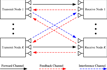
Figure 1: A model of MIMO interference network with limited CSI feedback.

We consider a MIMO interference network with $K$ transmitter-receiver links, as shown in Fig.1. For convenience of analysis, we assume a homogeneous system, where all transmitters and receivers are equipped with $N_{t}$ and $N_{r}$ antennas, respectively. While transmitter $k$ sends the signal to its intended receiver $k$, it also creates interference to other $K-1$ unintended receivers. We use $\alpha_{k,i}^{1/2}\textbf{H}_{k,i}$ to denote the channel from transmitter $i$ to receiver $k$, where $\alpha_{k,i}$ represents the path loss and $\textbf{H}_{k,i}$ is the $N_{r}\times N_{t}$ fast fading channel matrix with independent and identically distributed (i.i.d.) zero mean and unit variance complex Gaussian entries. Transmitter $k$ has $d_{k}$ independent data streams to be transmitted. It is worth pointing out that due to the limitation of spatial degree of freedom, the values of $d_{k}$s must fulfill the feasibility conditions of IA [25] [26]. In what follows, we assume IA is feasible by choosing $d_{k}$s carefully. Thus, the received signal at receiver $k$ can be expressed as

$$\textbf{y}_{k} = \sum\limits_{i=1}^{K}\sqrt{\frac{P\alpha_{k,i}}{d_{i}}}\textbf{H}_{k,i}\sum\limits_{l=1}^{d_{i}}\textbf{w}_{i,l}s_{i,l}+\textbf{n}_{k},$$ (1)

where $\textbf{y}_{k}$ is the $N_{r}$ dimensional received signal vector, $\textbf{n}_{k}$ is the additive Gaussian white noise with zero mean and covariance matrix $\sigma^{2}\textbf{I}_{N_{r}}$, $s_{i,l}$ denotes the $l$th normalized data stream from transmitter $i$, and $\textbf{w}_{i,l}$ is the corresponding $N_{t}$ dimensional beamforming vector. $P$ is the total transmit power at each transmitter, which is equally allocated to its data streams. Receiver $k$ uses the received vector $\textbf{v}_{k,j}$ of unit norm to detect its $j$th data stream, which is given by

$$\hat{s}_{k,j} = \textbf{v}_{k,j}^{H}\textbf{y}_{k}$$ (2)

$$= \sqrt{\frac{P\alpha_{k,k}}{d_{k}}}\textbf{v}_{k,j}^{H}\textbf{H}_{k,k}\textbf{w}_{k,j}s_{k,j}$$

$$+\sqrt{\frac{P\alpha_{k,k}}{d_{k}}}\sum\limits_{l=1,l\neq j}^{d_{k}}\textbf{v}_{k,j}^{H}\textbf{H}_{k,k}\textbf{w}_{k,l}s_{k,l}$$

$$+\sum\limits_{i=1,i\neq k}^{K}\sqrt{\frac{P\alpha_{k,i}}{d_{i}}}\sum\limits_{l=1}^{d_{i}}\textbf{v}_{k,j}^{H}\textbf{H}_{k,i}\textbf{w}_{i,l}s_{i,l}+\textbf{v}_{k,j}^{H}\textbf{n}_{k},$$

where the first term at the right side of (2) is the desired signal, the second one is the inter-stream interference caused by the same transmitter, and the third one is the inter-link interference resulting from the other transmitters. In order to mitigate these interferences and improve the performance, IA is performed accordingly. If perfect CSI is available at all nodes, we have

$$\textbf{v}_{k,j}^{H}\textbf{H}_{k,k}\textbf{w}_{k,l}=0,\quad l\neq j,\forall k\in[1,K],\forall l,j\in[1,d_{k}].$$ (3)

and

$$\textbf{v}_{k,j}^{H}\textbf{H}_{k,i}\textbf{w}_{i,l}=0,\quad i\neq k,\forall k,i\in[1,K],\forall l\in[1,d_{i}],\forall j\in[1,d_{k}].$$ (4)

In brief, inter-stream and inter-link interferences can be canceled completely if perfect CSI is available. However, in practical systems (e.g. frequency division duplex system), it is difficult for the transmitters to obtain full CSI, including the interference CSI. Since the feedback channel has limited bandwidth, codebook based quantization is an effective way to convey partial CSI from the receivers to the transmitters. In a MIMO interference network, CSI is quantized in the form of vectorization. Specifically, for the channel $\textbf{H}_{k,i}$, it is first vectorized as $\textbf{h}_{k,i}=\textmd{vec}(\textbf{H}_{k,i})$, then receiver $k$ selects an optimal codeword from a predetermined codebook $\mathcal{H}_{k,i}=\left\{\hat{\textbf{h}}_{k,i}^{(1)},\cdots,\hat{\textbf{h}}_{k,i}^{(2^{B_{k,i}})}\right\}$ of size $2^{B_{k,i}}$ according to the following criterion:

$$b^{\star}=\arg\max\limits_{1\leq b\leq 2^{B_{k,i}}}\left|\tilde{\textbf{h}}_{k,i}^{H}\hat{\textbf{h}}_{k,i}^{(b)}\right|^{2},$$ (5)

where $\tilde{\textbf{h}}_{k,i}=\textbf{h}_{k,i}/{\left\|\textbf{h}_{k,i}\right\|}$ is the channel direction vector. Transmitter $i$ recovers the quantized CSI from the same codebook $\mathcal{H}_{k,i}$ after receiving the feedback information $b^{\star}$, and then constructs its beamforming vectors $\textbf{w}_{i,l},l=1,\cdots,d_{i}$ based on all the feedback information about the related forward and interference channels, namely $\textbf{H}_{i,k},\forall k=1,\cdots,K$.

The MIMO interference network is operated in slotted time. At the beginning of each time slot, receiver $k$ conveys the optimal codeword index to transmitter $i$ with $B_{k,i}$ bits, where $i=1,\cdots,K$. It is worth pointing out that we consider a low mobility scenario, so the impact of feedback delay is negligible. Due to the limitation of feedback resource, we assume each receiver has $B$ feedback bits in total during one time slot. The focus of this paper is on performance analysis and optimization subject to $\sum\limits_{i=1}^{K}B_{k,i}=B$ for $k=1,\cdots,K$.

III Performance Analysis and Optimization

In this section, we concentrate on performance analysis and optimization for IA in a MIMO interference network with limited CSI feedback. In the case of limited CSI feedback, the capacity of MIMO interference network is still an open issue. For technical tractability, we alternatively put the attention on the average transmission rate. In the sequence, we first give a detailed investigation of average transmission rate, and then propose an adaptive feedback allocation scheme as well as a dynamic mode selection scheme for IA in a general MIMO interference network to optimize the overall performance.

III-A Average Transmission Rate

Due to limited CSI feedback, although IA is adopted, (3) and (4) do not hold true any more. These result in residual interference, also called interference leakage. Under such condition, the signal to interference plus noise ratio (SINR) related to the $j$th data stream of transmitter-receiver link $k$ can be expressed as

$$\gamma_{k,j} = \frac{\kappa_{k,k}\left|\textbf{v}_{k,j}^{H}\textbf{H}_{k,k}\textbf{w}_{k,j}\right|^{2}}{I_{k,j}+\sigma^{2}}$$ (6)

$$= \frac{\kappa_{k,k}\left|\textbf{h}_{k,k}^{H}\textbf{T}_{j,j}^{(k,k)}\right|^{2}}{I_{k,j}+\sigma^{2}},$$

where $\kappa_{k,k}=\frac{P\alpha_{k,k}}{d_{k}}$, $\textbf{T}_{j,j}^{(k,k)}=\textbf{w}_{k,i}\otimes\textbf{v}_{k,j}^{H}$ and $\otimes$ represents the Kronecker product. $I_{k,j}$ is the total residual interference, which is given by

$$I_{k,j} = \kappa_{k,k}\sum\limits_{l=1,l\neq j}^{d_{k}}\left|\textbf{v}_{k,j}^{H}\textbf{H}_{k,k}\textbf{w}_{k,l}\right|^{2}$$ (7)

$$+\sum\limits_{i=1,i\neq k}^{K}\kappa_{k,i}\sum\limits_{l=1}^{d_{i}}\left|\textbf{v}_{k,j}^{H}\textbf{H}_{k,i}\textbf{w}_{i,l}\right|^{2}$$

$$= \kappa_{k,k}\sum\limits_{l=1,l\neq j}^{d_{k}}\left|\textbf{h}_{k,k}^{H}\textbf{T}_{j,l}^{(k,k)}\right|^{2}$$

$$+\sum\limits_{i=1,i\neq k}^{K}\kappa_{k,i}\sum\limits_{l=1}^{d_{i}}\left|\textbf{h}_{k,i}^{H}\textbf{T}_{j,l}^{(k,i)}\right|^{2}$$

$$= \kappa_{k,k}\|\textbf{h}_{k,k}\|^{2}\sum\limits_{l=1,l\neq j}^{d_{k}}\left|\tilde{\textbf{h}}_{k,k}^{H}\textbf{T}_{j,l}^{(k,k)}\right|^{2}$$

$$+\sum\limits_{i=1,i\neq k}^{K}\kappa_{k,i}\|\textbf{h}_{k,i}\|^{2}\sum\limits_{l=1}^{d_{i}}\left|\tilde{\textbf{h}}_{k,i}^{H}\textbf{T}_{j,l}^{(k,i)}\right|^{2},$$

where $\kappa_{k,j}=\frac{P\alpha_{k,j}}{d_{j}}$ and $\textbf{T}_{j,l}^{(k,i)}=\textbf{w}_{i,l}\otimes\textbf{v}_{k,j}^{H}$. Following the theory of random vector quantization [27], the relation between the original channel direction vector $\tilde{\textbf{h}}_{k,i}$, and the quantized channel direction vector $\hat{\textbf{h}}_{k,i}$ can be expressed as

$$\tilde{\textbf{h}}_{k,i}=\sqrt{1-a_{k,i}}\hat{\textbf{h}}_{k,i}+\sqrt{a_{k,i}}\textbf{s}_{k,i},$$ (8)

where $a_{k,i}=\sin^{2}\left(\angle\left(\tilde{\textbf{h}}_{k,i},\hat{\textbf{h}}_{k,i}\right)\right)$ is the magnitude of the quantization error, and $\textbf{s}_{k,i}$ is an unit norm vector isotropically distributed in the nullspace of $\hat{\textbf{h}}_{k,i}$, and is independent of $a_{k,i}$. Since IA is performed based on the quantized CSI $\hat{\textbf{h}}_{k,i}$, so we have

$$\left|\tilde{\textbf{h}}_{k,i}^{H}\textbf{T}_{j,l}^{(k,i)}\right|^{2} = \left|\sqrt{1-a_{k,i}}\hat{\textbf{h}}_{k,i}^{H}\textbf{T}_{j,l}^{(k,i)}+\sqrt{a_{k,i}}\textbf{s}_{k,i}^{H}\textbf{T}_{j,l}^{(k,i)}\right|^{2}$$ (9)

$$= a_{k,i}\left|\textbf{s}_{k,i}^{H}\textbf{T}_{j,l}^{(k,i)}\right|^{2},$$

where (9) holds true according to the IA principles (3) and (4). In this case, the residual interference in (7) is reduced as

$$I_{k,j} = \kappa_{k,k}a_{k,k}\|\textbf{h}_{k,k}\|^{2}\sum\limits_{l=1,l\neq j}^{d_{k}}\left|\textbf{s}_{k,k}^{H}\textbf{T}_{j,l}^{(k,k)}\right|^{2}$$ (10)

$$+\sum\limits_{i=1,i\neq k}^{K}\kappa_{k,i}a_{k,i}\|\textbf{h}_{k,i}\|^{2}\sum\limits_{l=1}^{d_{i}}\left|\textbf{s}_{k,i}^{H}\textbf{T}_{j,l}^{(k,i)}\right|^{2},$$

where the first term at the right side is the residual inter-stream interference and the second term is the residual inter-link terms. In fact, the two kinds of interferences are equivalent if we consider each data stream as an independent link.

Hence, the average transmission rate for the $j$th data stream of transmitter-receiver link $k$ can be computed as

$$\bar{R}_{k,j} \!\!\!\!\!\!\!\!\!\!\!\!\!\!\!(\textbf{B}_{k},\textbf{d})$$ (13)

$$= E\left[\log_{2}\left(1+\gamma_{k,j}\right)\right]$$

$$= E\left[\log_{2}\left(\kappa_{k,k}\left|\textbf{h}_{k,k}^{H}\textbf{T}_{j,j}^{(k,k)}\right|^{2}+I_{k,j}+\sigma^{2}\right)\right]$$

$$-E\left[\log_{2}\left(I_{k,j}+\sigma^{2}\right)\right]$$

$$= \frac{1}{\ln 2}\sum\limits_{i=1}^{L}\sum\limits_{t=1}^{\eta_{k,i}}\Xi_{L}\Bigg{(}i,t,\{\eta_{k,q}\}_{q=1}^{L},$$

$$\left\{\frac{\varrho_{k,q}}{\eta_{k,i}}\right\}_{q=1}^{L},\{l_{k,q}\}_{q=1}^{L-2}\Bigg{)}Z\left(\sigma^{2},t,\frac{\varrho_{k,i}}{\eta_{k,i}}\right)$$

$$-\frac{1}{\ln 2}\sum\limits_{i=1}^{K}\sum\limits_{t=1}^{\omega_{k,i}}\Xi_{K}\Bigg{(}i,t,\{\omega_{k,q}\}_{q=1}^{K},$$

$$\left\{\frac{\varrho_{k,q}}{\omega_{k,i}}\right\}_{q=1}^{K},\{l_{k,q}\}_{q=1}^{K-2}\Bigg{)}Z\left(\sigma^{2},t,\frac{\varrho_{k,i}}{\omega_{k,i}}\right),$$

where

$$Z(x,y,z) = \ln(x)+\sum\limits_{\vartheta=0}^{y-1}\frac{1}{\Gamma(t-\vartheta)}\bigg{(}(-1)^{y-\vartheta-2}\left(\frac{x}{z}\right)^{y-\vartheta-1}$$

$$\times\exp\left(\frac{x}{z}\right)\textmd{E}_{\textmd{i}}\left(-\frac{x}{z}\right)$$

$$+\sum\limits_{\nu=1}^{y-\vartheta-1}\Gamma(\nu)\left(-\frac{x}{z}\right)^{y-\vartheta-\nu-1}\bigg{)},$$

$\textmd{E}_{\textmd{i}}(x)=\int_{-\infty}^{x}\frac{\exp(t)}{t}dt$ is the exponential integral function, $\textbf{B}_{k}=\{B_{k,1},\cdots,B_{k,K}\}$ is a certain feedback bits allocation result related to receiver $k$, and $\textbf{d}=\{d_{1},\cdots,d_{K}\}$ is a combination set on the numbers of data streams fulfilling the feasibility conditions [25] [26]. The proof of the above expression is presented in Appendix I.

Remark: It is found that (13) is independent of the data stream index $j$, since the desired signal quality and the residual interference are the same for all data streams of link $k$ in statistical sense. Therefore, the total rate of link $k$ is $d_{k}$ times $\bar{R}_{k,j}$, and thus the sum of average transmission rate for the MIMO interference network employing IA with limited CSI feedback is given by

$$\bar{R}(\textbf{B}_{k},\textbf{d}) = \sum\limits_{k=1}^{K}d_{k}\bar{R}_{k,j}(\textbf{B}_{k},\textbf{d}).$$ (14)

III-B Adaptive Feedback Allocation

As seen in (13), given channel conditions and the number of data streams, average transmission rate is a function of feedback bits $\textbf{B}_{k}$. In order to maximize the average transmission rate, it is necessary to distribute the feedback bits at each receiver, which is equivalent to the following optimization problem

$$J_{1}\!\!\!\!\! : \!\!\!\!\!\max\limits_{\textbf{B}_{k}}\bar{R}_{k,j}(\textbf{B}_{k},\textbf{d})$$ (15)

$$s.t. \sum\limits_{i=1}^{K}B_{k,i}=B$$ (16)

Evidently, $J_{1}$ is an integer programming problem and $\bar{R}_{k,j}(\textbf{B}_{k},\textbf{d})$ is a complicated function of $\textbf{B}_{k}$, so it is difficult to obtain a closed-form expression for the optimal solution. Intuitively, the optimal results can be achieved by using the numerical searching method, but the complexity increases proportionally with $K^{B}$, which is unbearable in practical systems with large $K$ and $B$. In order to get a balance between the performance and the complexity, we propose a greedy scheme to allocate the feedback resource bit by bit, and each bit is allocated to the channel that having $\bar{R}_{k,j}$ increases the fastest. The whole greedy feedback allocation scheme can be summarized as follows:

 

1. Initialization: Given $N_{t}$, $N_{r}$, $K$, $B$, $P$, $\sigma^{2}$, $d_{i}$ and $\alpha_{k,i}$ for $i=1,\cdots,K$. Let $B_{k,1}=\cdots=B_{k,K}=0$ and $\bar{R}_{k,j}(\textbf{B}_{k},\textbf{d})$ be defined as (13).

2. Let $\textbf{Q}^{(i)}=\{Q_{1},\cdots,Q_{K}\}$, where $Q_{j}=B_{k,j}$ for $j\neq i$, and $Q_{i}=B_{k,i}+1$. Search $i^{\star}=\max\limits_{1\leq i\leq K}\left(\bar{R}_{k,j}(\textbf{Q}^{(i)},\textbf{d})-\bar{R}_{k,j}(\textbf{B}_{k},\textbf{d})\right)$, then let $B_{k,i^{\star}}=B_{k,i^{\star}}+1$, $B=B-1$ and update $\textbf{B}_{k}$.

3. If $B>0$, then go to 2). Otherwise, $\textbf{B}_{k}$ is the feedback bits allocation result.

 

Note that the proposed scheme distributes each feedback bit by comparing $K$ rate increments, so the computational complexity is $\mathcal{O}(KB)$, which is simpler than the numerical search method. For an arbitrary receiver, the above scheme can also be used to obtain the feedback bits allocation result by substituting the corresponding network parameters.

III-C Dynamic Mode Selection

As seen in (14), the number of data streams $d_{i}$ has a great impact on the average transmission rate as well. While a larger $d_{i}$ leads to a higher multiplex gain, it also results in high interference. Hence, it is beneficial to select the optimal number of data stream, namely mode selection, from the perspective of the overall network performance. Taking the maximization of the sum of average transmission rate as the optimization objective, the problem of mode selection can be described as

$$J_{2}\!\!\!\!\! : \!\!\!\!\!\max\limits_{\textbf{d}}\bar{R}(\textbf{B}_{k},\textbf{d})$$ (17)

$$s.t. d_{i}\quad\text{satisfies the feasibility condition}\quad\forall i.$$ (18)

So far, the necessary and sufficient condition for the feasibility of IA for a general MIMO interference network is still an open problem. Since only the sufficient condition in the symmetric MIMO interference network is obtained, we consider the links that have the same number of data streams $d$, and change the constraint condition (18) as $N_{t}+N_{r}-(K+1)d\geq 0$ according to [25] and [26]. Thus, $J_{2}$, as an integer optimization problem, can be solved by the numerical searching method, and the total searching times is $\left\lfloor\frac{N_{t}+N_{r}}{K+1}\right\rfloor$, which is not so large in practical MIMO interference network with a limited number of antennas. For example, the maximum number of antennas for the LTE-A system is 8. Even if the link number is 4, the total searching number times is only 3. In particular, as verified by theoretical analysis and numerical simulation in the rest of this paper, the MIMO interference network either chooses $d=1$ or adopts the maximum feasible mode $d_{\max}=\left\lfloor\frac{N_{t}+N_{r}}{K+1}\right\rfloor$. Thus, we only need to compare the two transmission modes with bearable complexity.

III-D Joint Optimization Scheme

Feedback allocation and mode selection are integrally related. To be precise, given a feedback allocation result, there exists an optimal transmission mode combination. Similarly, a transmission mode combination corresponds to an optimal feedback allocation result. Hence, it is imperative to jointly optimize the two schemes, so as to maximize the sum of average transmission rate. In the sequence, we give a joint optimization scheme based on iteration as follows

 

1. Initialization: Given $N_{t}$, $N_{r}$, $K$, $B$, $P$, $\sigma^{2}$ and $\alpha_{k,i}$ for $i=1,\cdots,K$. Let $d_{1}=\cdots=d_{K}=d=1$ and $B_{k,1}=\cdots=B_{k,K}=0$;

2. Given d, perform feedback allocation to obtain $\textbf{B}_{k},\forall k\in[1,K]$;

3. Given $\textbf{B}_{k}$s, perform mode selection through searching $d$ from 1 to $d_{\max}$ to obtain d;

4. If nether $\textbf{B}_{k}$s nor d converge, go to 2). Otherwise, $\textbf{B}_{k}$s and d are the joint optimization results.

 

IV Asymptotic Analysis

In the last section, we have successfully derived the closed-form expression of the average transmission rate for IA with limited feedback in MIMO interference network, and presented two performance optimization schemes, namely adaptive feedback allocation and dynamic mode selection. A potential drawback is the high complexity of the expression and thus the optimization schemes. In order to obtain some insights on the system performance and hence extract several simple design guidelines, we carry out asymptotic performance analysis in two extreme cases, i.e. interference limited and noise limited. In what follows, we give a detailed investigation of average transmission rate and the corresponding performance optimization schemes in the two cases, respectively.

IV-A Interference Limited Case

If transmit power $P$ is large enough, the noise term of SINR in (6) can be negligible, thus the average transmission rate for the $j$th data stream of link $k$ is reduced as

$$\bar{R}_{k,j} \!\!\!\!\!\!\!\!\!\!\!\!\!\!\!(\textbf{B}_{k},\textbf{d})$$

$$= E\left[\log_{2}\left(\kappa_{k,k}\left|\textbf{h}_{k,k}^{H}\textbf{T}_{j,j}^{(k,k)}\right|^{2}+I_{k,j}\right)\right]$$

$$-E\left[\log_{2}\left(I_{k,j}\right)\right]$$

$$= \frac{1}{\ln 2}\bigg{(}\sum\limits_{i=1}^{L}\sum\limits_{t=1}^{\eta_{k,i}}\Xi_{L}\Bigg{(}i,t,\{\eta_{k,q}\}_{q=1}^{L},\left\{\frac{\varrho_{k,q}}{\eta_{k,i}}\right\}_{q=1}^{L-2},$$

$$\{l_{k,q}\}_{q=1}^{L-2}\Bigg{)}\left(\psi(t)+\ln(\varrho_{k,i})-\ln(\eta_{k,i})\right)$$

$$- \sum\limits_{i=1}^{K}\sum\limits_{t=1}^{\omega_{k,i}}\Xi_{K}\Bigg{(}i,t,\{\omega_{k,q}\}_{q=1}^{K},\left\{\frac{\varrho_{k,q}}{\omega_{k,i}}\right\}_{q=1}^{K},$$ (20)

$$\{l_{k,q}\}_{q=1}^{K-2}\Bigg{)}\left(\psi(t)+\ln(\varrho_{k,i})-\ln(\omega_{k,i})\right)\bigg{)},$$

where the proof of the above expression is presented in Appendix II. Then, the average transmission rate for the whole network is given by

$$\bar{R} \!\!\!\!\!\!\!\!\!\!\!\!\!\!\!(\textbf{B}_{k},\textbf{d})$$ (21)

$$= \sum\limits_{k=1}^{K}\frac{d_{k}}{\ln 2}\bigg{(}\sum\limits_{i=1}^{L}\sum\limits_{t=1}^{\eta_{k,i}}\Xi_{L}\Bigg{(}i,t,\{\eta_{k,q}\}_{q=1}^{L},$$

$$\left\{\frac{\varrho_{k,q}}{\eta_{k,i}}\right\}_{q=1}^{L-2}\Bigg{)}\left(\psi(t)+\ln(\varrho_{k,i})-\ln(\eta_{k,i})\right)$$

$$-\sum\limits_{i=1}^{K}\sum\limits_{t=1}^{\omega_{k,i}}\Xi_{K}\Bigg{(}i,t,\{\omega_{k,q}\}_{q=1}^{K},\left\{\frac{\varrho_{k,q}}{\omega_{k,i}}\right\}_{q=1}^{K},$$

$$\{l_{k,q}\}_{q=1}^{K-2}\Bigg{)}\left(\psi(t)+\ln(\varrho_{k,i})-\ln(\omega_{k,i})\right)\bigg{)}.$$

Substituting (20) into (15), and (21) into (17), we can get the corresponding feedback allocation and mode selection schemes.

Note that $\ln(\varrho_{k,i})=\ln(P)+\ln\left(\alpha_{k,i}2^{-\frac{B_{k,i}}{N_{t}N_{r}-1}}/d_{i}\right)$ $\forall i\in[1,K]$, $\ln(\varrho_{k,L})=\ln(P)+\ln\left(\alpha_{k,k}/d_{k}\right)$ and $\sum\limits_{i=1}^{L}\sum\limits_{t=1}^{\eta_{k,i}}\Xi_{L}\left(i,t,\{\eta_{k,q}\}_{q=1}^{L},\left\{\frac{\varrho_{k,q}}{\eta_{k,i}}\right\}_{q=1}^{L-2}\right)=1$ for arbitrary $L$ because of $\int_{0}^{\infty}f(x)=1$, so the terms related to $\ln(P)$ in $H(\textbf{B}_{k},\textbf{d})$ and $G(\textbf{B}_{k},\textbf{d})$ cancel out. Thus, we have the following theorem:

Theorem 1: In the region of high transmit power, the average transmission rate is independent of $P$, and there exists a performance ceiling regardless of $P$, i.e. once $P$ is larger than a saturation point, the average transmission rate will not increase further even the transmit power increases.

Intuitively, the performance ceiling is an increasing function of feedback bit $B$. To be precise, with the increase of $B$, the ceiling rises accordingly. Once $B$ is large enough, resulting in high SINR, then the constant term 1 in (13) can be negligible, then the average transmission rate can be approximated as

$$\bar{R}_{k,j}(\textbf{B}_{k},\textbf{d}) = E\left[\log_{2}\left(\kappa_{k,k}\left|\textbf{h}_{k,k}^{H}\textbf{T}_{j,j}^{(k,k)}\right|^{2}\right)\right]$$ (22)

$$-E\left[\log_{2}\left(I_{k,j}\right)\right],$$

If $B$ approaches infinity, namely perfect CSI at the transmitters, then the interference can be cancelled completely by IA. In this case, the average transmission rate can be expressed as

$$\bar{R}_{k,j}(\infty,\textbf{d}) = E\left[\log_{2}\left(\kappa_{k,k}\left|\textbf{h}_{k,k}^{H}\textbf{T}_{j,j}^{(k,k)}\right|^{2}\right)\right].$$ (23)

Therefore, the performance loss caused by limited CSI feedback under the condition of large $P$ and $B$ is given by

$$\Delta\bar{R}_{k,j} \!\!\!\!\!\!\!\!\!\!\!\!\!\!\!(\textbf{B}_{k},\textbf{d})$$ (25)

$$= \bar{R}_{k,j}(\infty,\textbf{d})-\bar{R}_{k,j}(\textbf{B}_{k},\textbf{d})$$

$$= E\left[\log_{2}\left(I_{k,j}\right)\right]$$

$$= \frac{1}{\ln(2)}\sum\limits_{i=1}^{K}\sum\limits_{t=1}^{\omega_{k,i}}\Xi_{K}\Bigg{(}i,t,\{\omega_{k,q}\}_{q=1}^{K},\left\{\frac{\varrho_{k,q}}{\omega_{k,i}}\right\}_{q=1}^{K},$$

$$\{l_{k,q}\}_{q=1}^{K-2}\Bigg{)}\left(\psi(t)+\ln(\varrho_{k,i})-\ln(\omega_{k,i})\right)$$

$$\approx \frac{1}{\ln(2)}\sum\limits_{i=1}^{K}\sum\limits_{t=1}^{\omega_{k,i}}\Xi_{K}\Bigg{(}i,t,\{\omega_{k,q}\}_{q=1}^{K},\left\{\frac{\varrho_{k,q}}{\omega_{k,i}}\right\}_{q=1}^{K},$$

$$\{l_{k,q}\}_{q=1}^{K-2}\Bigg{)}\ln(\varrho_{k,i})$$

$$= \frac{1}{\ln(2)}\sum\limits_{i=1}^{K}\sum\limits_{t=1}^{\omega_{k,i}}\Xi_{K}\Bigg{(}i,t,\{\omega_{k,q}\}_{q=1}^{K},\left\{\frac{\varrho_{k,q}}{\omega_{k,i}}\right\}_{q=1}^{K},$$

$$\{l_{k,q}\}_{q=1}^{K-2}\Bigg{)}\ln\left(P2^{-\frac{B_{i}}{N_{t}N_{r}-1}}\alpha_{k,i}/d_{i}\right),$$

where (25) follows the fact that $\psi(t)-\ln(\omega_{k,i})$ is negligible with respect to $\ln(\varrho_{k,i})$ when $P$ is large enough. Given $B$, the performance loss will enlarge as $P$ increases (due to performance ceiling mentioned above). In order to avoid the performance ceiling, $P2^{-\frac{B_{k,i}}{N_{t}N_{r}-1}}$ should remain constant. Hence, we have the following theorem:

Theorem 2: If the number of feedback bits satisfies $B=K(N_{t}N_{R}-1)\log_{2}\left(\frac{P}{\theta}\right)$, the performance gap between the full and limited CSI remains constant, where $\theta$ is a constant.

Proof:

As analyzed above, as long as $P2^{-\frac{B_{k,i}}{N_{t}N_{r}-1}}=\theta$ holds true, the performance loss is a constant. Equivalently, we have $B_{k,i}=(N_{t}N_{r}-1)\log_{2}\left(\frac{P}{\theta}\right)$, and then $B=\sum\limits_{i=1}^{K}B_{k,i}=K(N_{t}N_{R}-1)\log_{2}\left(\frac{P}{\theta}\right)$. ∎

From Theorem 2, we know that in order for the sum of average transmission rate under limited feedback to keep up the rate as perfect CSI feedback, $B$ needs to be increased as $P$ increases. Also from Theorem 2, it is found that with the increase of antenna number, in order to keep the constant performance gap, it is necessary to add more feedback bits. This is because when the number of antenna becomes large, the CSI quantization accuracy decreases accordingly, and there will be more residual interference. Furthermore, if we assume all links have the same number of data streams $d$, then the total performance loss due to limited CSI feedback can be expressed as

$$\Delta\bar{R}(\textbf{B}_{k},\textbf{d}) = d(\zeta_{1}-\zeta_{2}\ln(d)),$$ (26)

where $\zeta_{1}=\frac{1}{\ln(2)}\sum\limits_{k=1}^{K}\sum\limits_{i=1}^{K}\sum\limits_{t=1}^{\omega_{k,i}}\Xi_{K}\Bigg{(}i,t,\{\omega_{k,q}\}_{q=1}^{K},\left\{\frac{\varrho_{k,q}}{\omega_{k,i}}\right\}_{q=1}^{K},\\ \{l_{k,q}\}_{q=1}^{K-2}\Bigg{)}\ln\left(P2^{-\frac{B_{i}}{N_{t}N_{r}-1}}\alpha_{k,i}\right)$ and $\zeta_{2}=\frac{1}{\ln(2)}\sum\limits_{k=1}^{K}\sum\limits_{i=1}^{K}\sum\limits_{t=1}^{\omega_{k,i}}\Xi_{K}\left(i,t,\{\omega_{k,q}\}_{q=1}^{K},\left\{\frac{\varrho_{k,q}}{\omega_{k,i}}\right\}_{q=1}^{K},\{l_{k,q}\}_{q=1}^{K-2}\right)$. Since $\frac{\partial\Delta\bar{R}(\textbf{B}_{k},\textbf{d})}{\partial d}>0$, $\Delta\bar{R}(\textbf{B}_{k},\textbf{d})$ is an increasing function of $d$, we have the following theorem:

Theorem 3: In the case of large $P$ and $B$, $d=1$ is the asymptotically optimal transmission mode.

In fact, it is easy to understand that when the interference is so strong, single data stream transmission can decrease the residual interference significantly, and thus improves the performance.

IV-B Noise Limited Case

If the interference term is negligible with respect to the noise term due to the low transmit power, then the SINR is reduced as

$$\gamma_{k,j}=\frac{\kappa_{k,k}\left|\textbf{h}_{k,k}^{H}\textbf{T}_{j,j}^{(k,k)}\right|^{2}}{\sigma^{2}},$$ (27)

which is equivalent to the interference-free case. As discussed earlier, $\kappa_{k,k}\left|\textbf{h}_{k,k}^{H}\textbf{T}_{j,j}^{(k,k)}\right|^{2}$ is $\kappa_{k,k}\chi^{2}(2)$ distributed, then the average transmission rate can be computed as

$$\bar{R}_{k,j} = \int_{0}^{\infty}\log_{2}\left(1+\frac{x}{\sigma^{2}}\right)\frac{\exp(-x/\kappa_{k,k})}{\kappa_{k,k}}dx$$ (28)

$$= -\exp\left(\frac{\sigma^{2}}{\kappa_{k,k}}\right)\textmd{E}_{\textmd{i}}\left(-\frac{\sigma^{2}}{\kappa_{k,k}}\right).$$

It is found that $\bar{R}_{k,j}$ is independent of $B_{k,i}$ for all $i$. Thus, in the noise limited case, there is no need for CSI feedback, as CSI is useless for performance improvement.

In fact, the noise limited case can be considered as interference-free, so the interference CSI is immaterial. It has also been shown in [33] that at low SNR region, IA does not perform well as compared to the other interference mitigation schemes. It is easy to derive the sum of average transmission rate based on (28) as follows

$$\bar{R}=\sum\limits_{k=1}^{K}-d_{k}\exp\left(\frac{\sigma^{2}}{\kappa_{k,k}}\right)\textmd{E}_{\textmd{i}}\left(-\frac{\sigma^{2}}{\kappa_{k,k}}\right).$$ (29)

Note that (29) is an increasing function of $d_{k}$, so we also have the following theorem:

Theorem 4: It is optimal to use the maximum $d_{k}$ fulfilling the feasibility conditions of IA in the noise limited case.

As a simple example, for a symmetric MIMO interference network, $d=\left\lfloor\frac{N_{t}+N_{r}}{K+1}\right\rfloor$ is optimal under noise limited scenario. It is also aligned with the intuition that in an interference-free network, the spatial multiplexing gain should be exploited as much as possible. Similar phenomenon has also been observed in traditional multiuser downlink networks [31] [32].

V Numerical Results

To evaluate the accuracy of the performance analysis results, and the effectiveness of the performance optimization schemes for IA under a limited feedback MIMO interference networks, we present several simulation results under several different scenarios. For convenience, we set $N_{t}=8$, $N_{r}=8$, $K=4$, $B=20$, $\sigma^{2}=1$, $d_{1}=d_{2}=d_{3}=d_{4}=d=2$ and $\alpha_{i,j}$ given in Tab.I for all simulation scenarios without explicit explanation. In addition, we use SNR (in dB) to represent $10\log_{10}\frac{P}{\sigma^{2}}$. Without loss of generality, we take the sum of average transmission rate as the performance metric. We compare the proposed adaptive feedback allocation scheme (PAS) with two baseline schemes, namely equal feedback allocation scheme (EAS) and residual interference minimization based feedback allocation scheme (RIMS). As the name implies, EAS lets $B_{k,i}=B/K$ for all $k$ and $i$, and RIMS distributes the feedback bits based on the criterion of the minimization of average residual interference. Moreover, we also compare the performance of dynamic mode selection scheme and fixed mode scheme.

TABLE I: Parameter Table for $\alpha_{i,j},\forall i,j\in[1,4]$

	1	2	3	4
1	1.00	0.50	0.10	0.01
2	0.55	1.00	0.45	0.10
3	0.10	0.45	1.00	0.55
4	0.01	0.10	0.50	1.00

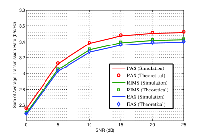
Figure 2: Performance comparison of different feedback bits allocation schemes

First, we compare the sum of average transmission rates of PAS, RIMS, and EAS. Note that we present both theoretical and simulation results for all the three schemes. As seen in Fig.2, the theoretical results nearly coincide with the simulation results in the whole SNR region, which testifies the high accuracy. From the performance point of view, PAS performs better than RIMS and EAS, since RIMS only considers the residual interference and EAS completely ignores the channel conditions. As SNR increases, the performance gain enlarges gradually. Therefore, PAS is an effective performance optimization scheme for IA with limited CSI feedback in the sense of maximizing the sum rate. It is worth pointing out that, with respect to PAS, EAS and RIMS have lower complexity. Specifically, EAS distributes the feedback bits equally, so the computational complexity is $\mathcal{O}(1)$. RIMS computes the feedback bits for each transmitter by maximizing the average residual interference [23] [24], thus the computational complexity is $\mathcal{O}(K)$. PAS allocates each feedback bit by comparing $K$ rate increments, so the computational complexity is $\mathcal{O}(KB)$. Clearly, the performance gain is achieved at the cost of complexity. In additional, it is found that there exist performance ceilings for all the three schemes in the high SNR region, which reconfirms Theorem 1. Furthermore, when the SNR is low, all three schemes have nearly the same performance, since the CSI feedback is useless in noise limited case as analyzed.

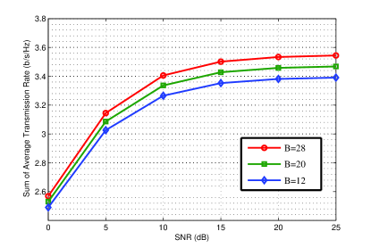
Figure 3: Performance comparison of PAS with different feedback bits

Secondly, we show the benefit of PAS from the perspective of feedback amount. As seen in Fig. 3, the performance gain from higher feedback amount becomes larger with the increase of SNR. Moreover, it is found that there always exists a performance ceiling for a given $B$ after a saturation point, but the ceiling will rise as $B$ increases. Thus, in order to avoid the ceiling, one should increase $B$ according to the claim in Theorem 2. In addition, there is hardly any performance gain in low SNR region even one increases $B$, which reconfirms the claim that CSI is useless at low SNR.

Next, we investigate the impact of the number of transmit antenna $N_{t}$ on the sum of average transmission rate for PAS. For a given feedback amount $B$, the performance degrades with the increase of the number of transmit antennas, this is because the quantization accuracy decreases, and the residual interference increases accordingly as explained in Theorem 2.

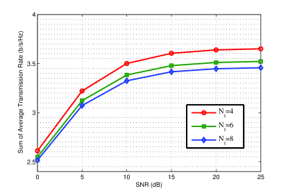
Figure 4: Performance comparison of LBS scheme with different number of transmit antennas and $B$=21

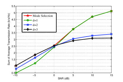
Figure 5: Performance comparison of mode selection scheme with fixed mode selection

Then, we compare the performance of dynamic mode selection scheme and fixed mode scheme based on PAS. As shown in Fig.5, dynamic mode selection scheme always obtains the optimal performance. For example, at SNR=10dB, dynamic mode selection scheme can get about $1.5$b/s/Hz gain with respect to fixed mode scheme of $d=2$. Thus, dynamic mode selection is a powerful performance optimization for IA with limited CSI feedback. Moreover, it is found that in the low SNR region, maximum feasible $d$ is chosen; while in the high SNR region, $d=1$ is optimal. These validate the claims in Theorem 4 and Theorem 3, respectively. More importantly, it is illustrated that only two transmission modes are adopted possibly, so we only need to compares the performances of the two modes when performing mode selection, which reduces the complexity significantly.

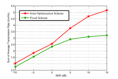
Figure 6: Performance comparison of combined optimization scheme with fixed scheme

Finally, we show the benefit of the proposed feedback allocation and mode selection joint optimization scheme over the EAS with $d=2$. As seen from Fig.6, even at very low SNR, the proposed combined optimization scheme can achieve significant performance gain. This is because the joint optimization scheme chooses the maximum transmission mode, which is optimal under this condition. With the increase of SNR, the performance gain becomes larger. For example, there is an about 2b/s/Hz gain at SNR=15dB. The performance gain comes from two folds: at high SNR, the network is interference limited, the joint optimization scheme selects single stream mode to decrease the interference; on the other hand, based on the optimal single stream mode, the joint optimization scheme uses all feedback bits to mitigate the inter-link interference, which increases the feedback utility efficiency. Hence, the proposed joint optimization scheme can effectively improve the performance of IA with limited CSI feedback.

VI Conclusion

This paper addresses the problem of performance analysis and optimization for IA in a general MIMO interference network with limited CSI feedback. A major contribution of this paper is having derived the closed-form expression of the average transmission rate in terms of feedback amount and transmission mode. Based on this result, we propose two feasible and effective performance optimization schemes, namely adaptive feedback allocation and dynamic mode selection. In addition, asymptotic analysis is carried out to obtain further insights on system performance and design guidelines. For example, our asymptotic results show that the number of feedback bits has to be increased when the transmit power is increased or when the number of antennas is increased; while under noise-limited scenario, the feedback of CSI have no impact on improving the system performance with IA, hence spatial degree of freedom should be exploited as much as possible. On the contrary, single data stream should be chosen in interference-limited scenario.

Appendix A The derivation of $\bar{R}_{k,j}(\textbf{B}_{k},\mathbf{d})$

Let $W(\textbf{B}_{k},\textbf{d})$ and $V(\textbf{B}_{k},\textbf{d})$ denote the first and second terms at the right hand of (13). At first, we put the focus on $W(\textbf{B}_{k},\textbf{d})$. By substituting (10) into (13), we have

$$W \!\!\!\!\!\!\!\!\!\!\!\!\!\!\!(\textbf{B}_{k},\textbf{d})$$

$$= \frac{1}{\ln 2}E\bigg{[}\ln\bigg{(}\kappa_{k,k}\left|\textbf{h}_{k,k}^{H}\textbf{T}_{j,j}^{(k,k)}\right|^{2}$$

$$+\kappa_{k,k}a_{k,k}\|\textbf{h}_{k,k}\|^{2}\sum\limits_{l=1,l\neq j}^{d_{k}}|\textbf{s}_{k,k}^{H}\textbf{T}_{j,l}^{(k,k)}|^{2}$$

$$+\sum\limits_{i=1,i\neq k}^{K}\kappa_{k,i}a_{k,i}\sum\limits_{l=1}^{d_{i}}\|\textbf{h}_{k,i}\|^{2}\left|\textbf{s}_{k,i}^{H}\textbf{T}_{j,l}^{(k,i)}\right|^{2}+\sigma^{2}\bigg{)}\bigg{]}.$$

According to the theory of quantization cell approximation [27], $a_{k,i}\|\textbf{h}_{k,i}\|^{2}$ is $\Gamma(N_{t}N_{r}-1,2^{-\frac{B_{k,i}}{N_{t}N_{r}-1}})$ distributed. Moreover, $|\textbf{s}_{k,i}^{H}\textbf{T}_{j,l}^{(k,i)}|^{2}$ for $i=1,\cdots,K$ are i.i.d. $\beta(1,N_{t}N_{r}-2)$ distributed, since $\textbf{T}_{j,l}^{(k,i)}$ of unit norm is independent of $\textbf{s}_{k,i}$. For the product of a $\Gamma(N_{t}N_{r}-1,2^{-\frac{B_{k,i}}{N_{t}N_{r}-1}})$ distributed random variable and a $\beta(1,N_{t}N_{r}-2)$ distributed random variable, it is equal to $2^{-\frac{B_{k,i}}{N_{t}N_{r}-1}}\chi^{2}(2)$ in distribution [28]. Based on the fact that the sum of $M$ i.i.d. $\chi^{2}(2)$ distributed random variables is $\chi^{2}(2M)$ distributed, $a_{k,i}\sum\limits_{l=1}^{d_{i}}\|\textbf{h}_{k,i}\|^{2}\left|\textbf{s}_{k,i}^{H}\textbf{T}_{j,l}^{(k,i)}\right|^{2}$ is $2^{-\frac{B_{k,i}}{N_{t}N_{r}-1}}\chi^{2}(2d_{i})$ distributed. Additionally, since $\textbf{T}_{j,j}^{(k,k)}$ is designed independently of $\textbf{h}_{k,k}$, $\left|\textbf{h}_{k,k}^{H}\textbf{T}_{j,j}^{(k,k)}\right|^{2}$ is also $\chi^{2}(2)$ distributed. Hence, $\kappa_{k,k}\left|\textbf{h}_{k,k}^{H}\textbf{T}_{j,j}^{(k,k)}\right|^{2}+\kappa_{k,k}a_{k,k}\|\textbf{h}_{k,k}\|^{2}\sum\limits_{l=1,l\neq j}^{d_{k}}|\textbf{s}_{k,k}^{H}\textbf{T}_{j,l}^{(k,k)}|^{2}+\sum\limits_{i=1,i\neq k}^{K}\kappa_{k,i}a_{k,i}\sum\limits_{l=1}^{d_{i}}\|\textbf{h}_{k,i}\|^{2}\left|\textbf{s}_{k,i}^{H}\textbf{T}_{j,l}^{(k,i)}\right|^{2}$ is a nested finite weighted sum of $K+1$ Erlang pdfs, whose pdf is given by [29]

$$f(x) = \sum\limits_{i=1}^{L}\sum\limits_{t=1}^{\eta_{k,i}}\Xi_{L}\left(i,t,\{\eta_{k,q}\}_{q=1}^{L},\left\{\frac{\varrho_{k,q}}{\eta_{k,q}}\right\}_{q=1}^{L},\{l_{k,q}\}_{q=1}^{L-2}\right)$$ (31)

$$\times g\left(x,t,\frac{\varrho_{k,i}}{\eta_{k,i}}\right),$$

where $L=K+1$, $\eta_{k,i}=d_{i}$, $\varrho_{k,i}=\kappa_{k,i}2^{-\frac{B_{k,i}}{N_{t}N_{r}-1}}$ for all $i\neq k$, $\eta_{k,k}=d_{k}-1$, $\varrho_{k,k}=\kappa_{k,k}2^{-\frac{B_{k,k}}{N_{t}N_{r}-1}}$, $\eta_{k,L}=1$, $\varrho_{k,L}=\kappa_{k,k}$, and $g(x,t,\varrho_{k,i})=\frac{x^{t-1}\exp(-x/\varrho_{k,i})}{\varrho_{k,i}^{t}\Gamma(t)}$ for all $i\in[1,L]$. The weights $\Xi_{L}$ are defined as

$$\Xi_{L}\!\!\!\!\!\!\! \!\!\!\!\!\!\!\left(i,t,\{\eta_{k,q}\}_{q=1}^{L},\{\varrho_{k,q}\}_{q=1}^{L},\{l_{k,q}\}_{q=1}^{L-2}\right)$$

$$= \sum\limits_{l_{k,1}=t}^{\eta_{k,i}}\sum\limits_{l_{k,2}=t}^{l_{k,1}}\cdots\sum\limits_{l_{k,L-2}=t}^{l_{k,L-3}}\bigg{[}\frac{(-1)^{T_{L}-\eta_{k,i}}\varrho_{k,i}^{t}}{\prod_{h=1}^{L}\varrho_{k,h}^{\eta_{k,h}}}$$

$$\times\frac{\Gamma(\eta_{k,i}+\eta_{k,1+\textmd{U}(1-i)}-l_{k,1})}{\Gamma(\eta_{k,1+\textmd{U}(1-i)})\Gamma(\eta_{k,i}-l_{k,1}+1)}$$

$$\times\left(\frac{1}{\varrho_{k,i}}-\frac{1}{\varrho_{k,1+\textmd{U}(1-i)}}\right)^{l_{k,1}-\eta_{k,i}-\eta_{k,1+\textmd{U}(1-i)}}$$

$$\times\frac{\Gamma(l_{k,L-2}+\eta_{k,L-1+\textmd{U}(L-1-i)}-t)}{\Gamma(\eta_{k,L-1+\textmd{U}(L-1-i)})\Gamma(l_{L-2}-t+1)}$$

$$\times\left(\frac{1}{\varrho_{k,i}}-\frac{1}{\varrho_{k,L-1+\textmd{U}(L-1-i)}}\right)^{t-l_{k,L-2}-\eta_{k,L-1+\textmd{U}(L-1-i)}}$$

$$\times\prod_{s=1}^{L-3}\frac{\Gamma(l_{k,s}+\eta_{k,s+1+\textmd{U}(s+1-i)}-l_{k,s+1})}{\Gamma(\eta_{k,s+1+\textmd{U}(s+1-i)})\Gamma(l_{k,s}-l_{k,s+1}+1)}$$

$$\times\left(\frac{1}{\varrho_{k,i}}-\frac{1}{\varrho_{k,s+1+\textmd{U}(s+1-i)}}\right)^{l_{k,s+1}-l_{k,s}-\eta_{k,s+1+\textmd{U}(s+1-i)}}\bigg{]},$$

where $T_{L}=\sum_{i=1}^{L}\eta_{k,i}$ and $\textmd{U}(x)$ is the well-known unit step function defined as $\textmd{U}(x\geq 0)=1$ and zero otherwise. Note that the weights $\Xi_{L}$ are constant when given $\eta_{k,i}$ and $\varrho_{k,i}$. Thus, $W(\textbf{B}_{k},\textbf{d})$ can be computed as

$$W \!\!\!\!\!\!\!\!\!\!\!\!\!\!\!(\textbf{B}_{k},\textbf{d})$$ (33)

$$= \frac{1}{\ln 2}\int_{0}^{\infty}\ln(x+\sigma^{2})f(x)dx$$

$$= \frac{1}{\ln 2}\sum\limits_{i=1}^{L}\sum\limits_{t=1}^{\eta_{k,i}}\Xi_{L}\Bigg{(}i,t,\{\eta_{k,q}\}_{q=1}^{L},\left\{\frac{\varrho_{k,q}}{\eta_{k,q}}\right\}_{q=1}^{L},$$

$$\{l_{k,q}\}_{q=1}^{L-2}\Bigg{)}\int_{0}^{\infty}\ln(x+\sigma^{2})g\left(x,t,\frac{\varrho_{k,i}}{\eta_{k,i}}\right)dx$$

$$= \frac{1}{\ln 2}\sum\limits_{i=1}^{L}\sum\limits_{t=1}^{\eta_{k,i}}\Xi_{L}\Bigg{(}i,t,\{\eta_{k,q}\}_{q=1}^{L},\left\{\frac{\varrho_{k,q}}{\eta_{k,q}}\right\}_{q=1}^{L},$$

$$\{l_{k,q}\}_{q=1}^{L-2}\Bigg{)}Z\left(\sigma^{2},t,\frac{\varrho_{k,i}}{\eta_{k,i}}\right),$$

where

$$Z \!\!\!\!\!\!\!\!\!\!\!\!\!\!\!\left(\sigma^{2},t,\frac{\varrho_{k,i}}{\eta_{k,i}}\right)$$ (34)

$$= \int_{0}^{\infty}\ln(x+\sigma^{2})g\left(x,t,\frac{\varrho_{k,i}}{\eta_{k,i}}\right)dx$$

$$= \ln(\sigma^{2})+\sum\limits_{\vartheta=0}^{t-1}\frac{1}{\Gamma(t-\vartheta)}\bigg{(}(-1)^{t-\vartheta-2}\left(\frac{\sigma^{2}\eta_{k,i}}{\varrho_{k,i}}\right)^{t-\vartheta-1}$$

$$\times\exp\left(\frac{\sigma^{2}\eta_{k,i}}{\varrho_{k,i}}\right)\textmd{E}_{\textmd{i}}\left(-\frac{\sigma^{2}\eta_{k,i}}{\varrho_{k,i}}\right)$$

$$+\sum\limits_{\nu=1}^{t-\vartheta-1}\Gamma(\nu)\left(-\frac{\sigma^{2}\eta_{k,i}}{\varrho_{k,i}}\right)^{t-\vartheta-\nu-1}\bigg{)},$$

and $\textmd{E}_{\textmd{i}}(x)=\int_{-\infty}^{x}\frac{\exp(t)}{t}dt$ is the exponential integral function. (34) follows from [30, Eq. 4.3375].

Note that $V(\textbf{B}_{k},\textbf{d})$ is similar to $W(\textbf{B}_{k},\textbf{d})$ except the absence of the term $\kappa_{k,k}\left|\textbf{h}_{k,k}^{H}\textbf{T}_{j,j}^{(k,k)}\right|^{2}$. Hence, $V(\textbf{B}_{k},\textbf{d})$ can be expressed as

$$V(\textbf{B}_{k},\textbf{d}) = \frac{1}{\ln 2}\sum\limits_{i=1}^{K}\sum\limits_{t=1}^{\omega_{k,i}}\Xi_{K}\Bigg{(}i,t,\{\omega_{k,q}\}_{q=1}^{K},\left\{\frac{\varrho_{k,q}}{\omega_{k,i}}\right\}_{q=1}^{K},$$ (35)

$$\{l_{k,q}\}_{q=1}^{K-2}\Bigg{)}Z\left(\sigma^{2},t,\frac{\varrho_{k,i}}{\omega_{k,i}}\right),$$

where $\omega_{k,k}=d_{k}-1$, $\omega_{k,i}=d_{i}$ for $i\neq k$, and $\varrho_{k,i}=\kappa_{k,i}2^{-\frac{B_{k,i}}{N_{t}N_{r}-1}}$ for all $i\in[1,K]$. So, we obtain the average transmission rate for the $j$th data stream of link $k$ as follows

$$\bar{R}_{k,j} \!\!\!\!\!\!\!\!\!\!\!\!\!\!\!(\textbf{B}_{k},\textbf{d})$$

$$= W(\textbf{B}_{k},\textbf{d})-V(\textbf{B}_{k},\textbf{d})$$

$$= \frac{1}{\ln 2}\sum\limits_{i=1}^{L}\sum\limits_{t=1}^{\eta_{k,i}}\Xi_{L}\Bigg{(}i,t,\{\eta_{k,q}\}_{q=1}^{L},\left\{\frac{\varrho_{k,q}}{\eta_{k,i}}\right\}_{q=1}^{L},$$

$$\{l_{k,q}\}_{q=1}^{L-2}\Bigg{)}Z\left(\sigma^{2},t,\frac{\varrho_{k,i}}{\eta_{k,i}}\right)$$

$$-\frac{1}{\ln 2}\sum\limits_{i=1}^{K}\sum\limits_{t=1}^{\omega_{k,i}}\Xi_{K}\Bigg{(}i,t,\{\omega_{k,q}\}_{q=1}^{K},\left\{\frac{\varrho_{k,q}}{\omega_{k,i}}\right\}_{q=1}^{K},$$

$$\{l_{k,q}\}_{q=1}^{K-2}\Bigg{)}Z\left(\sigma^{2},t,\frac{\varrho_{k,i}}{\omega_{k,i}}\right).$$ (36)

Appendix B The derivation of $\bar{R}_{k,j}(\textbf{B}_{k},\mathbf{d})$ in interference limited case

For convenience, we use $G(\textbf{B}_{k},\textbf{d})$ and $H(\textbf{B}_{k},\textbf{d})$ to denote the first and second terms at the right hand of (IV-A). The pdf of $\kappa_{k,k}\left|\textbf{h}_{k,k}^{H}\textbf{T}_{j,j}^{(k,k)}\right|^{2}+I_{k,j}$ is given by $f(x)$ in (31), thus $G(\textbf{B}_{k},\textbf{d})$ can be computed as

$$G \!\!\!\!\!\!\!\!\!\!\!\!\!\!\!(\textbf{B}_{k},\textbf{d})$$ (37)

$$= \frac{1}{\ln 2}\int_{0}^{\infty}\ln(x)f(x)dx$$

$$= \frac{1}{\ln 2}\sum\limits_{i=1}^{L}\sum\limits_{t=1}^{\eta_{k,i}}\Xi_{L}\Bigg{(}i,t,\{\eta_{k,q}\}_{q=1}^{L},\left\{\frac{\varrho_{k,q}}{\eta_{k,i}}\right\}_{q=1}^{L},$$

$$\{l_{k,q}\}_{q=1}^{L-2}\Bigg{)}\int_{0}^{\infty}\ln(x)\frac{x^{t-1}\exp(-\frac{x}{\varrho_{k,i}/\eta_{k,i}})}{(\varrho_{k,i}/\eta_{k,i})^{t}\Gamma(t)}dx$$

$$= \frac{1}{\ln 2}\sum\limits_{i=1}^{L}\sum\limits_{t=1}^{\eta_{k,i}}\Xi_{L}\Bigg{(}i,t,\{\eta_{k,q}\}_{q=1}^{L},\left\{\frac{\varrho_{k,q}}{\eta_{k,i}}\right\}_{q=1}^{L},$$

$$\{l_{k,q}\}_{q=1}^{L-2}\Bigg{)}\left(\psi(t)+\ln(\varrho_{k,i})-\ln(\eta_{k,i})\right),$$

where $\psi(x)=\frac{d\ln(\Gamma(x))}{dx}$ is the Euler psi function. (37) is obtained based on [30, Eq. 4.352.1]. Similarly, we can get $H(\textbf{B}_{k},\textbf{d})$ as follows:

$$H(\textbf{B}_{k},\textbf{d}) = \frac{1}{\ln 2}\sum\limits_{i=1}^{K}\sum\limits_{t=1}^{\omega_{k,i}}\Xi_{K}\Bigg{(}i,t,\{\omega_{k,q}\}_{q=1}^{K},\left\{\frac{\varrho_{k,q}}{\omega_{k,i}}\right\}_{q=1}^{K},$$ (38)

$$\{l_{k,q}\}_{q=1}^{K-2}\Bigg{)}\left(\psi(t)+\ln(\varrho_{k,i})-\ln(\omega_{k,i})\right).$$

Hence, the average transmission rates for the $j$th data stream of link $k$ is given by

$$\bar{R}_{k,j} \!\!\!\!\!\!\!\!\!\!\!\!\!\!\!(\textbf{B}_{k},\textbf{d})$$ (39)

$$= \frac{1}{\ln 2}\bigg{(}\sum\limits_{i=1}^{L}\sum\limits_{t=1}^{\eta_{k,i}}\Xi_{L}\Bigg{(}i,t,\{\eta_{k,q}\}_{q=1}^{L},\left\{\frac{\varrho_{k,q}}{\eta_{k,i}}\right\}_{q=1}^{L-2},$$

$$\{l_{k,q}\}_{q=1}^{L-2}\Bigg{)}\left(\psi(t)+\ln(\varrho_{k,i})-\ln(\eta_{k,i})\right)$$

$$- \sum\limits_{i=1}^{K}\sum\limits_{t=1}^{\omega_{k,i}}\Xi_{K}\Bigg{(}i,t,\{\omega_{k,q}\}_{q=1}^{K},\left\{\frac{\varrho_{k,q}}{\omega_{k,i}}\right\}_{q=1}^{K},$$

$$\{l_{k,q}\}_{q=1}^{K-2}\Bigg{)}\left(\psi(t)+\ln(\varrho_{k,i})-\ln(\omega_{k,i})\right)\bigg{)},$$

References

• [1] V. R. Cadambe, and S. A. Jafar, “Interference alignment and degrees of freedom of the K-user interference channel,” IEEE Trans. Inf. Theory, vol. 54, no. 8, pp. 3425-3441, Aug. 2008.
• [2] M. A. Maddah-Ali, A. S. Motahari, and A. K. Khandani, “Communication over MIMO X channels: interferece alignment, decomposition, and performance analysis,” IEEE Trans Inf. Theory, vol. 54, no. 8, pp. 3457-3470, Aug. 2008.
• [3] H. Ning, C. Ling, and K. K. Leung, “Feasibility condition for interference alignment with diversity,” IEEE Trans. Inf. Theory, vol. 57, no. 5, pp. 2902-2912, Feb. 2011.
• [4] H. Yu, and Y. Sung, “Least squares approach to joint beam design for interference alignment in multiuser multi-input multi-output interference channels,” IEEE Trans. Signal Process., vol. 58, no. 9, pp. 4960-4966, Feb. 2010.
• [5] P. Mohapatra, K. E. Nissar, and C. R. Murthy, “Interference alignment algorithms for the K user constant MIMO interference channel,” IEEE Trans. Signal Process., vol. 59, no. 11, pp. 5499-5508, Feb. 2011.
• [6] K. Huang, and R. Zhang, “Cooperative precoding with limited feedback for MIMO interference channels,” IEEE Trans. Wireless Commun., vol. 11, no. 3, pp. 1012-1021, Mar. 2012.
• [7] A. S. Motahari, and A. K. Khandani, “Capcity bounds for the Gaussian interference channel,” IEEE Trans. Inf. Theory, vol. 55, no. 2, pp. 620-643, Feb. 2009.
• [8] X. Shang, G. Kramer, and B. Chan, “A new outer bound and the noisy-interference sum-rate capacity for Gaussian interference channels,” IEEE Trans. Inf. Theory, vol. 55, no. 2, pp. 689-699, Feb. 2009.
• [9] K. Gomadam, V. R. Cadambe, and S. A. Jafar, “A distributed numberical approach to interference alignment and applications to wireless interference networks,” IEEE Trans. Inf. Theory, vol. 57, no. 6, pp. 3309-3322, Jun. 2011.
• [10] C. Suh, and D. Tse, “Interference alignment for cellular networks,” in Proc. 46th Annual Allerton Conf. Commun., Control, Comput., Sep. 2008.
• [11] C. Suh, M. Ho, D. Tse, “Downlink interference alignment,” IEEE Trans. Commun., vol. 59, no. 9, pp. 2616-2626, Sep. 2011.
• [12] B. Jung, and W. Shin, “Opportunistic interference alignment for interfernce-limited cellular TDD uplink,” IEEE Commun. Lett., vol. 15, no. 2, pp. 148-151, Feb. 2011.
• [13] H. Huang, V. K. N. Lau, Y. Du, and S. Liu, “Robust lattice alignment for K-user MIMO interference channels with imperfect channel knowledge,” IEEE Trans. Signal Process., vol. 59, no. 7, Jul. 2011.
• [14] S. A. Jafar, “Blind interference alignment,” IEEE J. Sel. Topics Signal Process., vol. 6, no. 3, pp. 216-227, Jun. 2012.
• [15] D. J. Love, R. W. Heath Jr., V. K. N. Lau, D. Gesbert, B. D. Rao, and M. Andrews, “An overview of limited feedback in wireless communication systems,” IEEE J. Sel. Areas Commun.,, vol. 26, no. 8, pp. 1341-1365, Oct. 2008.
• [16] H. Bolcskei, and I. J. Thukral, “Interference alignment with limited feedback,” In Proc. IEEE ISIT, pp. 1759-1763, Jun. 2009.
• [17] X. Chen, and H-H. Chen, “Interference-aware resource control in multi-antenna cognitive ad hoc networks with heterogeneous delay constraint,” IEEE Commun. Lett., vol. 17, no. 6, pp. 1184-1187, Jun. 2013.
• [18] R. T. Krishnamachari, and M. K. Varanasi, “Interference alignment under limited feedback for MIMO interference channels, IEEE Trans. Signal Process., vol. 61, no. 15, pp. 3908-3917, Aug. 2013.
• [19] S. Cho, K. Huang, D. Kim, and H. Seo, “Interference alignment for uplink cellular systems with limited feedback,” IEEE Commun. Lett., vol. 16, no. 7, pp. 960-963, May 2012.
• [20] J. Kim, S. Moon, S. Lee, and I. Lee, “A new channel quantization strategy for MIMO interference alignment with limited feedback,” IEEE Trans. Wireless Commun., vol. 11, no. 1, pp. 358-366, Jan. 2012.
• [21] H. Farhadi, C. Wang, and M. Skoglund, “On the throughput of wireless interference networks with limited feedback,” in Proc. IEEE ISIT, pp. 762-766, Jun. 2011.
• [22] K. Anand, E. Gunawan, and Y. Guan, “Beamformer design for the MIMO interference channels under limited channel feedback,” IEEE Trans. Commun., vol. 61, no. 8, pp. 3246-3258, Aug. 2013.
• [23] S. Cho, H. Chae, K. Huang, D. Kim, V. K. N. Lau, and H. Seo, “Efficienct feedback design for interference alignment in MIMO interference channel,” in Proc. IEEE VTC, pp. 1-5, Jun. 2012.
• [24] X. Rao, L. Ruan, and V. K. N. Lau, “Limited feedback design for interference alignment on MIMO interference networks with heterogeneous path loss and spatial correlations,” IEEE Trans. Sigal Process., vol. 61, no. 10, pp. 2598-2601, Oct. 2013.
• [25] C. M. Yetis, T, Gou, S. A. Jafar, and A. H. Hayran, “On feasibility of interference alignment in MIMO interference networks,” IEEE Trans. Signal Process., vol. 58, no. 9, pp. 4771-4782, Sep. 2010.
• [26] L. Ruan, V. K. N. Lau, and M. Z. Win, “The feasibility conditions for interference alignment in MIMO Networks,” IEEE Trans. Signal Process., vol. 61, no. 8, pp. 2066-2077, Aug. 2013.
• [27] N. Jindal, “MIMO Broadcast channels with finite-rate feedback,” IEEE Trans. Inf. Theory, vol. 52, no. 11, pp. 5045-5060, Nov. 2006.
• [28] K. K. Mukkavilli, A. Sabharwal, E. Erkip, and B. Aazhang, “On beamforming with finite rate feedback in multiple-antenna systems,” IEEE Trans. Inf. Theory, vol. 49, no. 10, pp. 2562-2579, Oct. 2003.
• [29] G. K. Karagiannidis, N. C. Sagias, and T. A. Tsiftsis, “Closed-form statistics for the sum of squared Nakagami-m variates and its application,” IEEE Trans. Commun., vol. 54, no. 8, pp. 1353-1359, Aug. 2006.
• [30] I. S. Gradshteyn, and I. M. Ryzhik, “Tables of intergrals, series, and products,” Acedemic Press, USA, 2007.
• [31] X. Chen, Z. Zhang, S. Chen, and C. Wang, “Adaptive mode selection for multiuser MIMO downlink employing rateless codes with QoS provisioning,” IEEE Trans. Wireless Commun., vol. 11, no. 2, pp. 790-799, Feb. 2012.
• [32] J. Zhang, M. Kountouris, J. G. Andrews, and R. W. Heath Jr., “Multi-mode transmission for the MIMO broadcast channel with imperfect channel state information,” IEEE Trans. Commun., vol. 59, no. 3, pp. 803-814, Mar. 2011.
• [33] J. Leithon, C. Yuen, H. A. Suraweera, and H. Gao, “A new opportunistic interference alignment scheme and performance comparison of MIMO interference alignment with limited feedback,” in Proc. Globecom - Workshop on Multicell Cooperation, pp. 1123-1127, Dec. 2012.