Anomalous Josephson effect induced by spin-orbit interaction and Zeeman effect in semiconductor nanowires

Abstract

We investigate theoretically the Josephson junction of semiconductor nanowire with strong spin-orbit (SO) interaction in the presence of magnetic field. By using a tight-binding model, the energy levels $E_{n}$ of Andreev bound states are numerically calculated as a function of phase difference $\varphi$ between two superconductors in the case of short junctions. The DC Josephson current is evaluated from the Andreev levels. In the absence of SO interaction, a $0$-$\pi$ transition due to the magnetic field is clearly observed. In the presence of SO interaction, the coexistence of SO interaction and Zeeman effect results in $E_{n}(-\varphi)\neq E_{n}(\varphi)$, where the anomalous Josephson current flows even at $\varphi=0$. In addition, the direction-dependence of critical current is observed, in accordance with experimental results.

I INTRODUCTION

The spin-orbit (SO) interaction in narrow-gap semiconductors, e.g., InAs and InSb, Winkler attracts a lot of interest in recent studies. The SO interaction gives a possibility of electrical spin manipulation, which is a great advantage for spintronic devices. Zutic For conduction electrons in direct-gap semiconductors, the SO interaction is expressed as

$$H_{\rm SO}=\frac{\lambda}{\hbar}\bm{\sigma}\cdot\left[\bm{p}\times\bm{\nabla}V(\bm{r})\right],$$ (1)

where $V(\bm{r})$ is an external potential and $\bm{\sigma}$ indicates the electron spin $\bm{s}=\bm{\sigma}/2$. In experiments of quantum well using such materials, strong SO interaction was reported. Nitta ; Grundler ; Yamada For an external electric field ${\cal E}$ perpendicular to the quantum well, the substitution of $V(\bm{r})=e{\cal E}z$ into Eq. (1) yields

$$H_{\rm SO}=\frac{\alpha}{\hbar}(p_{y}\sigma_{x}-p_{x}\sigma_{y}),$$ (2)

which is called the Rashba interaction. Here, the coupling constant $\alpha=e{\cal E}\lambda$ is tunable by an electric field, or a gate voltage.

The development of fabrication technique enables to construct various quantum systems with SO interaction. Particularly, semiconductor nanowires of InAs and InSb are investigated intensively, in which quantum point contacts and quantum dots can be formed. Fasth ; Pfund ; Nadj-Perge ; Nadj-Perge2 ; Nadj-Perge3 ; Schroer Indeed, the electrical manipulation of single electron spins was reported for quantum dots fabricated on the nanowires. Nadj-Perge2 ; Nadj-Perge3 ; Schroer In recent studies, the nanowire-superconductor hybrid systems were studied for searching the Majorana fermions. Mourik ; Rokhinson ; Das ; Deng The DC Josephson effect was also studied when the nanowires are connected to two superconductors (S/NW/S junctions). Doh ; Dam ; Nilsson

The Josephson effect is one of the most fundamental phenomena concerning quantum phase. In a Josephson junction, the supercurrent flows when the phase difference $\varphi$ between two superconductors is present. For the junction using normal metals or semiconductors, the electron and hole in the normal region are coherently coupled to each other by the Andreev reflections at normal / superconductor interfaces. Andreev The Andreev bound states, which have discrete energy levels $E_{n}$ (Andreev levels), are formed in the normal region around the Fermi level within the superconducting energy gap $\Delta_{0}$. Beenakker1 ; NazarovBlanter The Cooper pair transports via the Andreev bound states. For short junctions, where a distance $L$ between two superconductors is much smaller than the coherent length $\xi$ in the normal region, the Josephson current $I(\varphi)$ is determined by the Andreev levels. Beenakker1 ; Bardeen ; Furusaki1 ; Furusaki2 $\xi=\hbar v_{\rm F}/(\pi\Delta_{0})\equiv\xi_{0}$ for ballistic systems and $\xi=(\xi_{0}l_{0})^{1/2}$ for diffusive ones, where $v_{\rm F}$ is the Fermi velocity and $l_{0}$ is the mean free path. For the transmission probability $T_{n}$ of conduction channel $n$ ($=1,2,\cdots,N$) in the normal region, the current is written as

$$I(\varphi)=\frac{e\Delta_{0}}{2\hbar}\sum_{n=1}^{N}\frac{T_{n}\sin\varphi}{[1-T_{n}\sin^{2}(\varphi/2)]^{1/2}}.$$ (3)

Here, the current satisfies $I(-\varphi)=-I(\varphi)$. In the limit of low transparent junction, the current in Eq. (3) becomes $I(\varphi)\simeq I_{0}\sin\varphi$ with $I_{0}\equiv e\Delta_{0}/(2\hbar)\sum_{n}T_{n}$.

In superconductor / ferromagnet / superconductor (S/F/S) junctions, the oscillation of critical current accompanying a $0$-$\pi$ transition was observed as a function of the thickness of ferromagnet. Buzdin1 ; Kontos ; Ryazanov ; Oboznov The $0$- and $\pi$-states mean that the free energy is minimal at $\varphi=0$ and $\pi$, respectively. The $0$-$\pi$ transition is caused by the interplay between the spin-singlet correlation of the superconductivity and the exchange interaction in ferromagnet. The exchange interaction makes the spin-dependent phase shift in the propagation through the ferromagnet. Since the Andreev bound state consists of a right-going (left-going) electron with spin $\sigma$ and a left-going (right-going) hole with spin $-\sigma$, the phase shift modulates the Andreev levels. When the length of ferromagnet is increased, the $0$-$\pi$ transition takes place at the cusps of critical current. Oboznov A similar transition was observed recently in S/NW/S junctions with fixed length when the Zeeman splitting was tuned by applying a magnetic field. private

The effect of SO interaction in the Josephson junctions is an interesting subject, where many phenomena were predicted, e.g., fractional Josephson effect FuKane and anomalous supercurrent. Buzdin2 The fractional Josephson effect is a $4\pi$ periodicity of current phase relation, $I(\varphi)\sim\sin(\varphi/2)$, which is a property of Majorana fermions induced by the SO interaction in the superconducting region. The anomalous supercurrent is a finite supercurrent at zero phase difference, $I(\varphi=0)\neq 0$, which is induced by the breaking of symmetry of current phase relation. The symmetry breaking is attributed to the existence of SO interaction and magnetic field in the normal region.

In the present study, we focus on the anomalous Josephson current. The DC Josephson current with SO interaction in the normal region was investigated theoretically by a lot of groups, for normal metal with magnetic impurities, Buzdin2 two-dimensional electron gas (2DEG) in semiconductor heterostructures, Bezuglyi ; Liu2 ; Liu1 ; Liu3 ; Malshukov1 ; Malshukov2 ; Malshukov3 open quantum dots, Beri quantum dots with tunnel barriers, DellAnna ; Zazunov ; Dolcini ; Karrasch ; Droste ; Padurariu ; Brunetti carbon nanotubes, Lim quantum wires or nanowires, Krive1 ; Krive2 ; Cheng ; YEN quantum point contacts, Reynoso1 ; Reynoso2 topological insulators, Tanaka and others. Chtchelkatchev2 The SO interaction breaks the spin-degeneracy of Andreev levels when the time reversal symmetry is broken by the phase difference $\varphi\neq 0$ even in the absence of magnetic field. Beri ; Chtchelkatchev2 The splitting due to the SO interaction is obtained in the long junctions, $L\gg\xi$ (or intermediated-length junctions, $L\gtrsim\xi$). In the short junctions, however, the spin-degeneracy of Andreev levels holds. Beri ; Chtchelkatchev2 In both cases, the relation of $I(-\varphi)=-I(\varphi)$ is not broken, which means no supercurrent at $\varphi=0$.

In the presence of magnetic field, the SO interaction modifies qualitatively the current phase relation. Then, the anomalous Josephson current is obtained. Buzdin2 ; Liu1 ; Liu3 ; Zazunov ; Brunetti ; Krive1 ; Reynoso1 ; Reynoso2 ; YEN The anomalous current flows in so-called $\varphi_{0}$-state in which the free energy has a minimum at $\varphi=\varphi_{0}$ ($\neq 0,\pi$). comphi0 The anomalous Josephson current was predicted when the length of normal region $L$ is longer than or comparable to the coherent length $\xi$. Krive et al. derived the anomalous current for long junctions with a single conduction channel. Krive1 Reynoso et al. found the anomalous current through a quantum point contact in the 2DEG for $L\gtrsim\xi$. Reynoso1 ; Reynoso2 They discussed an influence of spin polarization induced around the quantum point contact with SO interaction EtoQPC on the Josephson current. They also showed the direction-dependence of critical current when a few conduction channels take part in the transport. In the experiment on the S/NW/S junctions, private the direction-dependent supercurrent was observed for samples of $L\gtrsim\xi$ in a parallel magnetic field to the nanowire, besides the above-mentioned $0$-$\pi$ transition. This should be ascribable to the strong SO interaction in the nanowires although the anomalous Josephson current was not examined.

In our previous paper, we investigated theoretically the DC Josephson effect in semiconductor nanowires with strong SO interaction in the case of short junction. YEN We examined a simple model with single scatterer to capture the physics of $0$-$\pi$ transition and anomalous Josephson effect. In our model, both elastic scatterings by the impurities and SO interaction in the nanowire were represented by the single scatterer. The Zeeman effect by a magnetic field shifts the wavenumber as $k_{\pm}^{>}=k_{\rm F}+(E\pm E_{\rm Z})/(\hbar v_{\rm F})$ for $k>0$ and $k_{\pm}^{<}=-k_{\rm F}-(E\pm E_{\rm Z})/(\hbar v_{\rm F})$ for $k<0$. Chtchelkatchev1 $E$ is an energy measured from the Fermi level. $E_{\rm Z}\equiv|g\mu_{B}B|/2$ is the Zeeman energy. The orbital magnetization is neglected in the nanowire. The Fermi velocity $v_{\rm F}$ is independent of channels. When $k>0$ ($k<0$), the electron and hole move to the right (left) and left (right), respectively. The propagation of electron with spin $\sigma=\pm$ and hole with $\sigma=\mp$ acquires the phase $\pm\theta_{B}=\pm|g\mu_{\rm B}B|L/(\hbar v_{\rm F})$. The term of $2EL/(\hbar v_{\rm F})$ is safely disregarded for short junctions. The terms of $k_{\rm F}$ are canceled out by each other. The simple model showed the oscillation of critical current with increase of $\theta_{B}$. The $0$- and $\pi$-states are realized when $\theta_{B}\sim 0$ and $\pi$, respectively. Around $\theta_{B}=\pi/2$, the $0$-$\pi$ transition takes place. In the presence of SO interaction, the anomalous Josephson current was obtained, which result means a realization of $\varphi_{0}$-state. Moreover, the direction-dependence of critical current is found. The critical current indicates cusps at the local minima. The position of cusps also depends on the current direction, in accordance with the experiment. private Between the cusps for positive and negative current direction, the transition from $\varphi_{0}\approx 0$ to $\approx\pi$ takes place.

In this paper, we study the anomalous Josephson effect numerically using a tight-binding model for the nanowire in the case of short junction. The purposes are to confirm our previous simple model and to elucidate the key ingredients of anomalous Josephson effect. First, we consider the case without SO interaction. The Andreev levels are invariant against the $\varphi$-inversion, $E_{n}(-\varphi)=E_{n}(\varphi)$. As a result, the current satisfies $I(-\varphi)=-I(\varphi)$ and hence no anomalous current is found. The critical current oscillates as a function of magnetic field accompanying the $0$-$\pi$ transition, which is characterized by a single parameter $\theta_{B}$ even for $N>1$. Next, we investigate the Josephson effect in the presence of SO interaction and Zeeman effect. The relation of $I(-\varphi)=-I(\varphi)$ is broken. As a result, the anomalous Josephson current and the direction dependence of critical current are obtained, which are qualitatively the same as those of single scatterer model. We stress that the spin-dependent channel mixing due to SO interaction plays an important role on the anomalous Josephson effect.

The organization of this paper is as follows. In Sec. II, we explain our model for the S/NW/S Josephson junction and calculation method of the Andreev levels and Josephson current. Numerical results are given in Sec. III. The last section (Sec. IV) is devoted to the conclusions and discussion.

II MODEL AND CALCULATION

In this section, we explain our model depicted in Fig. 1. We introduce the Bogoliubov-de Gennes (BdG) equation to obtain the Andreev levels. The formulation of solving BdG equation is given in terms of scattering matrix. Beenakker1 We apply the tight-binding model to the normal region, where the scattering matrices of conduction electrons and holes are numerically calculated. Datta ; Ando

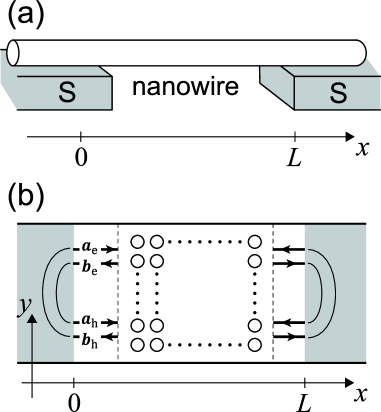
Figure 1: Our model for a quasi-one-dimensional semiconductor nanowire connected to two superconductors. The nanowire is along the $x$ axis. (a) Schematic view of the model. The pair potential is induced in the nanowire by the proximity effect, $\Delta(x)=\Delta_{0}e^{i\varphi_{\rm L}}$ at $x<0$ and $\Delta_{0}e^{i\varphi_{\rm R}}$ at $L<x$, whereas $\Delta(x)=0$ at $0<x<L$. Several impurities are present in the nanowire. The spin-orbit interaction and Zeeman effect are taken into account only in the normal region. (b) The tight-binding model gives the scattering matrix $\hat{S}_{\rm e}$ ($\hat{S}_{\rm h}$) for electrons (holes), which connects incoming $\bm{a}_{\rm e}$ ($\bm{a}_{\rm h}$) and outgoing electrons $\bm{b}_{\rm e}$ (holes $\bm{b}_{\rm h}$). At $x=0$ and $L$, the electron $\bm{b}_{\rm e}$ is reflected as the hole $\bm{a}_{\rm h}$ by the Andreev reflection, whereas $\bm{b}_{\rm h}$ is reflected as $\bm{a}_{\rm e}$.

II.1 Formulation

We consider a semiconductor nanowire along the $x$ axis connected to two superconductors at $x<0$ and $x>L$, as shown in Fig. 1(a). The superconducting pair potential is penetrated into the nanowire by the proximity effect, whereas there is no pair potential in the normal region at $0<x<L$. The SO interaction and Zeeman effect in a magnetic field are taken into account only in the normal region. Since InSb has a large g-factor, a large Zeeman energy is obtained for weak magnetic field, which does not break the superconductivity.

The Andreev bound states are formed in the normal region. The BdG equation to describe the Andreev bound states is written as Blonder ; NazarovBlanter

$$\left(\begin{array}[]{cc}H-E_{\rm F}&\hat{\Delta}\\ \hat{\Delta}^{\dagger}&-(H^{*}-E_{\rm F})\end{array}\right)\left(\begin{array}[]{c}\bm{\psi}_{\rm e}\\ \bm{\psi}_{\rm h}\end{array}\right)=E\left(\begin{array}[]{c}\bm{\psi}_{\rm e}\\ \bm{\psi}_{\rm h}\end{array}\right),$$ (4)

where $\bm{\psi}_{\rm e}=(\psi_{{\rm e}+},\psi_{{\rm e}-})^{\rm T}$ and $\bm{\psi}_{\rm h}=(\psi_{{\rm h}+},\psi_{{\rm h}-})^{\rm T}$ are the spinors for electron and hole, respectively. The energy $E$ is measured from the Fermi level $E_{\rm F}$. The diagonal element is the single-electron Hamiltonian $H=H_{0}+H_{\rm SO}+H_{\rm Z}$ with $H_{0}=\bm{p}^{2}/(2m^{*})+V_{\rm conf}(y,z)+V_{\rm imp}$, SO interaction $H_{\rm SO}$, and Zeeman effect $H_{\rm Z}=g\mu_{\rm B}{\bm{B}}\cdot\hat{\bm{\sigma}}/2$, using effective mass $m^{*}$, $g$-factor $g$ ($<0$ for InSb), Bohr magneton $\mu_{\rm B}$, and Pauli matrices $\hat{\bm{\sigma}}$. $H_{\rm SO}$ and $H_{\rm Z}$ are taken into account only at $0<x<L$. $V_{\rm conf}$ describes the confining potential of nanowire. $V_{\rm imp}$ represents the potential due to the impurities. $\hat{\Delta}$ is the pair potential in the spinor space

$$\hat{\Delta}=\Delta(x)\hat{g}=\Delta(x)\left(\begin{array}[]{cc}&-1\\ 1&\end{array}\right),$$ (5)

where $\hat{g}=-i\hat{\sigma}_{y}$. com1 For simplicity, we assume that the absolute values of pair potential in left and right superconducting regions are equal to each other, $\Delta(x)=\Delta_{0}e^{i\varphi_{\rm L}}$ at $x<0$ and $\Delta_{0}e^{i\varphi_{\rm R}}$ at $L<x$. In the normal region at $0<x<L$, $\Delta(x)=0$. The phase difference between two superconductors is defined as $\varphi\equiv\varphi_{\rm L}-\varphi_{\rm R}$. We consider a short junction, where $L\ll\xi$. No potential barrier is assumed at the boundaries between the normal and superconducting regions. The Zeeman energy $E_{\rm Z}\equiv|g\mu_{B}B|/2$ and the pair potential $\Delta_{0}$ are much smaller than the Fermi energy $E_{\rm F}$.

The solution of BdG equation gives the Andreev levels $E_{n}$ ($|E_{n}|<\Delta_{0}$) as a function of phase difference $\varphi$. When the BdG equation has an eigenenergy $E_{n}$ with eigenvector $(\bm{\psi}_{{\rm e},n},\bm{\psi}_{{\rm h},n})^{\rm T}$, $-E_{n}$ is also an eigenenergy of the equation with $(\bm{\psi}_{{\rm h},n}^{*},\bm{\psi}_{{\rm e},n}^{*})^{\rm T}$. In short junctions, the number of Andreev levels is given by $4N$; $2N$ positive levels and $2N$ negative ones when the number of channels is $N$ ($2N$ if the spin degree of freedom is included). The ground-state energy of the junction is given by

$$E_{\rm gs}(\varphi)=-\frac{1}{2}{\sum_{n}}^{\prime}E_{n}(\varphi),$$ (6)

where the summation is taken over all the positive Andreev levels, $E_{n}(\varphi)>0$. The contribution from continuous levels ($|E|>\Delta_{0}$) is disregarded in Eq. (6), which are independent of $\varphi$ in the short junctions. Beenakker1 At zero temperature, the supercurrent is calculated as

$$I(\varphi)=\frac{2e}{\hbar}\frac{dE_{\rm gs}}{d\varphi}=-\frac{e}{\hbar}{\sum_{n}}^{\prime}\frac{dE_{n}}{d\varphi}.$$ (7)

The current is a periodic function for $-\pi<\varphi\leq\pi$. The maximum (absolute value of minimum) of $I(\varphi)$ yields the critical current $I_{{\rm c},+}$ ($I_{{\rm c},-}$) in the positive (negative) direction.

The symmetry of BdG equation should be noted here. We denote the matrix on the left side of Eq. (4) by $\mathcal{H}(\varphi)$. In the absence of Zeeman effect, $\mathcal{T}\mathcal{H}(\varphi)\mathcal{T}^{-1}=\mathcal{H}(-\varphi)$ with the time-reversal operator $\mathcal{T}=-i\hat{\sigma}_{y}K$ for spin-1/2 particles. $K$ is the operator to form a complex conjugate; $Kf=f^{*}$. If $\mathcal{H}(\varphi)$ has an eigenenergy $E_{n}$ with eigenvector $(\bm{\psi}_{{\rm e},n},\bm{\psi}_{{\rm h},n})^{\rm T}$, $\mathcal{H}(-\varphi)$ has an eigenenergy $E_{n}$ with eigenvector $\mathcal{T}(\bm{\psi}_{{\rm e},n},\bm{\psi}_{{\rm h},n})^{\rm T}$. Thus the Andreev levels satisfy the relation of $E_{n}(\varphi)=E_{n}(-\varphi)$. In the absence of SO interaction, $K\mathcal{H}(\varphi)K^{-1}=\mathcal{H}(-\varphi)$. Then we derive that $E_{n}(\varphi)=E_{n}(-\varphi)$ in the same way. The relation does not always hold in the presence of both SO interaction and magnetic field.

II.2 Scattering Matrix Approach

The BdG equation in Eq. (4) can be written in terms of the scattering matrix. Beenakker1

In the normal region with SO interaction and Zeeman effect, the quantum transport of electrons (holes) is described by the scattering matrix $S_{\rm e}$ ($S_{\rm h}$). The scattering matrix $S_{\rm p}$ (${\rm p}={\rm e,h}$) connects the amplitudes of incoming waves of $N$ conduction channels with spin $\sigma=\pm$, $(\bm{a}_{\rm pL},\bm{a}_{\rm pR})^{\rm T}$, and those of outgoing waves, $(\bm{b}_{\rm pL},\bm{b}_{\rm pR})^{\rm T}$, as shown in Fig. 1(b),

$$\left(\begin{array}[]{c}\bm{b}_{\rm pL}\\ \bm{b}_{\rm pR}\end{array}\right)=\hat{S}_{\rm p}\left(\begin{array}[]{c}\bm{a}_{\rm pL}\\ \bm{a}_{\rm pR}\end{array}\right).$$ (8)

$\hat{S}_{\rm e}$ and $\hat{S}_{\rm h}$ are $4N\times 4N$ matrices and related to each other by $\hat{S}_{\rm e}(E)=\hat{S}_{\rm h}^{*}(-E)$. On the assumption that they are independent of energy $E$ for $|E|<\Delta_{0}$, and thus $\hat{S}_{\rm e}=\hat{S}_{\rm h}^{*}$. We denote $\hat{S}_{\rm e}=\hat{S}$ and $\hat{S}_{\rm h}=\hat{S}^{*}$. $\hat{S}$ is conventionally written by reflection and transmission matrices:

$$\hat{S}=\left(\begin{array}[]{cc}\hat{r}_{\rm L}&\hat{t}_{\rm LR}\\ \hat{t}_{\rm RL}&\hat{r}_{\rm R}\end{array}\right).$$ (9)

The scattering matrix is unitary, $\hat{S}^{\dagger}\hat{S}=\hat{1}$. Moreover, $\hat{r}_{\rm L}^{\rm T}=\hat{g}^{\dagger}\hat{r}_{\rm L}\hat{g}$, $\hat{r}_{\rm R}^{\rm T}=\hat{g}^{\dagger}\hat{r}_{\rm R}\hat{g}$, and $\hat{t}_{\rm RL}^{\rm T}=\hat{g}^{\dagger}\hat{t}_{\rm LR}\hat{g}$ are satisfied if the time reversal symmetry is kept.

The Andreev reflection at $x=0$ and $L$ is also described in terms of scattering matrix $\hat{r}_{\rm he}$ for the conversion from electron to hole and $\hat{r}_{\rm eh}$ for that from hole to electron. When an electron with spin $\sigma$ is reflected into a hole with $-\sigma$, it is written as Beenakker1

$$\left(\begin{array}[]{c}\bm{a}_{\rm hL}\\ \bm{a}_{\rm hR}\end{array}\right)=\hat{r}_{\rm he}\left(\begin{array}[]{c}\bm{b}_{\rm eL}\\ \bm{b}_{\rm eR}\end{array}\right),$$ (10)

where

$$\hat{r}_{\rm he}=e^{-i\alpha_{\rm A}}\left(\begin{array}[]{cc}e^{-i\varphi_{\rm L}}\hat{1}\otimes\hat{g}&\\ &e^{-i\varphi_{\rm R}}\hat{1}\otimes\hat{g}\end{array}\right)$$ (11)

with $\alpha_{\rm A}\equiv\arccos(E/\Delta_{0})$. When a hole is reflected to an electron, it is

$$\left(\begin{array}[]{c}\bm{a}_{\rm eL}\\ \bm{a}_{\rm eR}\end{array}\right)=\hat{r}_{\rm eh}\left(\begin{array}[]{c}\bm{b}_{\rm hL}\\ \bm{b}_{\rm hR}\end{array}\right)$$ (12)

with

$$\hat{r}_{\rm eh}=e^{-i\alpha_{\rm A}}\left(\begin{array}[]{cc}e^{i\varphi_{\rm L}}\hat{1}\otimes\hat{g}^{\dagger}&\\ &e^{i\varphi_{\rm R}}\hat{1}\otimes\hat{g}^{\dagger}\end{array}\right).$$ (13)

We assume that the channel is conserved at the Andreev reflection in the case of $N\geq 2$. The normal reflection can be neglected in our case without potential barriers at the boundaries. Andreev

The product of scattering matrices gives an equation for $(\bm{a}_{\rm eL},\bm{a}_{\rm eR})^{\rm T}$. The Andreev levels $E_{n}(\varphi)$ are calculated from this product as, Beenakker1

$$\det\left(\hat{1}-\hat{r}_{\rm eh}\hat{S}^{*}\hat{r}_{\rm he}\hat{S}\right)=0,$$ (14)

which is equivalent with the BdG equation in Eq. (4). In the absence of magnetic field, Eq. (14) is simply reduced to Beenakker1

$$\det\left[1-\left(\frac{E}{\Delta_{0}}\right)^{2}-\hat{t}_{\rm LR}^{\dagger}\hat{t}_{\rm LR}\sin^{2}\left(\frac{\varphi}{2}\right)\right]=0.$$ (15)

In this case, the Andreev levels are represented by the transmission eigenvalues of $\hat{t}_{\rm LR}^{\dagger}\hat{t}_{\rm LR}$. They are two-fold degenerate reflecting the Kramers’ degeneracy at $\varphi=0$. The Andreev levels $E_{n}(\varphi)$ are not split by finite $\varphi$ in spite of the broken time reversal symmetry.

II.3 Tight-Binding Model

To obtain the scattering matrix $\hat{S}$, we describe the normal region by a tight-binding model of square lattice model in two-dimensional space ($xy$ plane), Datta as schematically shown in Fig. 1(b). We consider a quasi-one-dimensional nanowire along the $x$ axis with width $W$ in the $y$ direction. The length of normal region is $L$. We assume hard-wall potentials at $y=0$ and $W$. The Rashba-type SO interaction in Eq. (2) and the Zeeman effect are considered in the normal region. The Rashba interaction specifies the direction of spin quantization axis. In the experiments, the nanowire is not two-dimensional or the SO interaction may not be Rashba one. However, our model is general to represent a single or few conduction channels in the nanowire and to consider the spin mixing among channels by the SO interaction. In the following, the magnetic field is applied in the $y$ direction, which is almost parallel to the spin quantization axis due to the Rashba interaction for the channels. The channel is split upward and downward by the Zeeman effect. The orbital magnetization is neglected.

On the tight-binding model, the Hamiltonian $H=H_{0}+H_{\rm SO}+H_{\rm Z}$ is written as

$$H = t\sum_{j,l}\bm{c}_{j,l}^{\dagger}\left\{(4+v_{j,l})\hat{1}+\bm{b}\cdot\hat{\bm{\sigma}}\right\}\bm{c}_{j,l}$$ (16)

$$-t\sum_{j,l}\left(\bm{c}_{j,l}^{\dagger}\hat{T}_{j,l;j+1,l}\bm{c}_{j+1,l}+\bm{c}_{j,l}^{\dagger}\hat{T}_{j,l;j,l+1}\bm{c}_{j,l+1}+\text{H.\ c.}\right),$$

where $\bm{c}_{j,l}\equiv(c_{j,l;+},c_{j,l;-})^{\rm T}$ and $c_{j,l;\sigma}$ is annihilation operator of an electron at site $(j,l)$ with spin $\sigma$. $t\equiv\hbar^{2}/(2m^{*}a^{2})$ is a transfer integral with a lattice constant $a$. Here, $j$ ($=0,1,\cdots,N_{x},N_{x}+1$) and $l$ ($=1,2,\cdots,N_{y}$) denote site labels in the $x$ and $y$ directions, respectively. The length is $L=N_{x}a$ and the width is $W=(N_{y}+1)a$. At the sites of $j=0,N_{x}+1$, the SO interaction and Zeeman effect is absent. $v_{j,l}\equiv V_{j,l}/t$ is a dimensionless on-site potential by impurities. $\hat{1}$ is the unit matrix in the spinor space. $\bm{b}\equiv g\mu_{\rm B}\bm{B}/(2t)$ indicates a magnetic field. The transfer term in the $x$ direction is given by

$$\hat{T}_{j,l;j+1,l}=\hat{1}-ik_{\alpha}a\hat{\sigma}_{y},$$ (17)

whereas that in the $y$ direction is

$$\hat{T}_{j,l;j,l+1}=\hat{1}+ik_{\alpha}a\hat{\sigma}_{x}.$$ (18)

Here, $k_{\alpha}=m^{*}\alpha/\hbar^{2}$ denotes the strength of Rashba interaction. In this model, the reflection and transmission matrices are calculated by using the recursive Green’s function method (see Appendix A). Ando

We set the Fermi wavelength $\lambda_{\rm F}$ as a parameter, which gives the Fermi energy by $E_{\rm F}=2t-2t\cos(k_{\rm F}a)$ with $k_{\rm F}=2\pi/\lambda_{\rm F}$. comSO In an ideal quantum wire with width $W$, the dispersion relation for channel $n$ is given by

$$E_{n}(k)=4t-2t\cos(ka)-2t\cos\left(\frac{\pi a}{W}n\right).$$ (19)

The conduction channels satisfy $E_{n}(k=0)<E_{\rm F}$. Then, the velocity of channel $n$ at the Fermi energy is

$$v_{{\rm F},n}=\frac{2ta}{\hbar}\sqrt{1-\left\{2-\cos\left(\frac{\pi a}{W}n\right)-\frac{E_{\rm F}}{2t}\right\}^{2}}.$$ (20)

We consider a nanowire with width $W=60\,\mathrm{nm}$. The distance between left and right superconductors is $L=1000\,\mathrm{nm}$. We set $N_{x}=11$ and $N_{y}=200$. The number of conduction channel is changed by tuning the Fermi wavenumber $\lambda_{\rm F}$. In the following, we calculate for three cases: $\lambda_{\rm F}=90\,\mathrm{nm}$ for single channel ($N=1$), $50\,\mathrm{nm}$ for $N=2$, and $25\,\mathrm{nm}$ for $N=4$. A parameter of Rashba interaction is $k_{\alpha}/k_{\rm F}=0.15$. The on-site random potential by impurities is uniformly distributed in $-W_{0}/2<V_{j,l}<W_{0}/2$. The mean free path $l_{0}$ is estimated as Ando

$$l_{0}=\frac{6\lambda_{\rm F}^{3}}{\pi^{3}a^{2}}\left(\frac{E_{\rm F}^{\prime}}{W_{0}}\right)^{2}.$$ (21)

Here we use the modified Fermi energy $E_{\rm F}^{\prime}=E_{\rm F}-E_{1}(0)$ in an one-dimensional quantum wire.

III NUMERICAL RESULTS

In this section, we present calculated results of Andreev levels and Josephson currents. First, we discuss the case without SO interaction. The critical current oscillates as a function of magnetic field and the $0$-$\pi$ transition is clearly found. Next, we consider the anomalous Josephson effect induced by the SO interaction.

The magnetic field is applied in the $y$ direction. We introduce a parameter of magnetic field, $\theta_{B}=|g|\mu_{\rm B}BL/(\hbar\bar{v}_{\rm F})$, where $\bar{v}_{\rm F}\equiv\left\{(1/N)\sum_{n=1}^{N}(1/v_{{\rm F},n})\right\}^{-1}$ is the inversion average of velocity $v_{{\rm F},n}$ in Eq. (20). The Zeeman effect splits the dispersion relation for spin $\sigma=\pm$. The wavenumber becomes $k_{{\rm F},n,\pm}\simeq k_{{\rm F},n}\pm|g|\mu_{\rm B}B/(2\hbar v_{{\rm F},n})$ for $k>0$ and $k_{{\rm F},n,\pm}\simeq-k_{{\rm F},n}\mp|g|\mu_{\rm B}B/(2\hbar v_{{\rm F},n})$ for $k<0$. For the propagation of electron with spin $\sigma=\pm$ and hole with $\sigma=\mp$ in the normal region, the shift of phase due to the Zeeman effect is $\pm|g|\mu_{\rm B}BL/(\hbar v_{{\rm F},n})$. Therefore, $\theta_{B}$ means the channel-average of spin-dependent phase shift of electron and hole forming the Andreev bound states.

III.1 Absence of spin-orbit interaction

III.1.1 Single conduction channel

Figure 2: Calculated results for a sample when $N=1$ and $l_{0}/L=1$. The SO interaction is absent. (a) Andreev levels $E_{n}$ as a function of phase difference $\varphi$ between two superconductors. Solid and broken lines indicate $E_{\uparrow i\pm}$ and $E_{\downarrow i\pm}$, respectively. The magnetic field is $\theta_{B}=0$ (left upper), $0.1\pi$ (left middle), $0.27\pi$ (left bottom), $0.53\pi$ (right upper), $0.79\pi$ (right middle), and $\pi$ (right bottom). At $B=0$, two lines are overlapped to each other, reflecting the Kramers’ degeneracy. (b) Josephson current $I(\varphi)$ through the nanowire when $\theta_{B}=0$ (solid), $0.27\pi$ (broken), $0.53\pi$ (dotted), and $\pi$ (dotted broken lines).

First, we consider a sample of nanowire with a single conduction channel. Figure 2 shows the Andreev levels and Josephson currents as functions of phase difference $\varphi$ between two superconductors. The magnetic field gradually increases from left-upper to right-bottom panels. In the absence of SO interaction, the spin $\sigma=\pm$ is well defined in the direction of magnetic field. In the case of single conduction channel, four Andreev levels are found in $|E|\leq\Delta_{0}$. The levels are denoted as $E_{\uparrow i\pm}$ and $E_{\downarrow i\pm}$, where the subscript $\uparrow$ ($\downarrow$) means the state of electron spin $\sigma=+1$ ($\sigma=-1$) and hole spin $\sigma=-1$ ($\sigma=+1$). $i=1,2,\cdots$. The sign $\pm$ corresponds to the positive or negative energy at $B=0$. We consider three regions with increasing $\theta_{B}$. When $B=0$, the levels are doubly degenerate for any $\varphi$. The ground-state energy $E_{\rm gs}$ becomes minimal at $\varphi=0$, which corresponds to the $0$-state [Fig. 3(a)]. The levels are split like the Zeeman splitting in the presence of magnetic field. For a weak magnetic field, $E_{\rm gs}$ is still minimal at $\varphi=0$ [region (I)]. As the magnetic field is increased, the level crossing at $E=0$ is observed, which corresponds to region (II). The crossing points move from $\varphi=\pm\pi$ to $0$ with increase of $\theta_{B}$. When $\theta_{B}\approx\pi$, no level crossing takes place in region (III). In this region, $E_{\rm gs}$ is minimal at $\varphi=\pi$ ($\pi$-state). The transition of $0$-state to $\pi$-state takes place suddenly around $\theta_{B}=\pi/2$, as shown in Fig. 3(a). This is called the $0$-$\pi$ transition. With increase of magnetic field, some levels go to $|E|>\Delta_{0}$. At the same time, another levels come into $|E|\leq\Delta_{0}$. Therefore, the number of Andreev levels in $|E|\leq\Delta_{0}$ is fixed.

The Josephson current is calculated from the sum of positive Andreev levels in Eq. (7). In Fig. 2(a), the Andreev levels $E_{n}(\varphi)$ are invariant against the inversion of $\varphi$, $E_{n}(-\varphi)=E_{n}(\varphi)$. As a result, the Josephson current satisfies $I(-\varphi)=-I(\varphi)$ in Fig. 2(b). When $\theta_{B}=0$, the current $I(\varphi)$ is similar to $\sin\varphi$, which is a feature of $0$-state. When the level crossing takes place at $E=0$, the crossing results in the discontinuity in the current phase relation. Around $\theta_{B}=\pi/2$, a saw-tooth current phase relation is obtained. The discontinuous points move from $\pm\pi$ to $0$. When $\theta_{B}\approx\pi$, the current is roughly $I(\varphi)\sim-\sin\varphi$, which is a feature of $\pi$-state.

Figure 3: Calculated results for $N=1$ and $l_{0}/L=1$. The SO interaction is absent. (a) Phase difference $\varphi_{0}$ at the minimum of ground-state energy as a function of magnetic field, $\theta_{B}$. (b) Critical current $I_{{\rm c},\pm}$. The current in the positive direction $I_{{\rm c},+}$ is identical with that in the negative direction $I_{{\rm c},-}$. The sample for (a) and (b) is same as that in Fig. 2. (c) Average of critical current, $\langle I_{{\rm c},\pm}\rangle$, with the average of fluctuation, $\sqrt{\langle[\Delta I_{{\rm c},\pm}]^{2}\rangle}$, as error bars, where $\Delta I_{{\rm c},\pm}\equiv I_{{\rm c},\pm}-\langle I_{{\rm c},\pm}\rangle$. The random average is taken for 400 samples.

Figure 3(b) shows the critical current as a function of $\theta_{B}$. Since $I(-\varphi)=-I(\varphi)$, the maximum of Josephson current, $I_{{\rm c},+}$, is identical with the absolute value of minimum of current, $I_{{\rm c},-}$. When the magnetic field is stronger, the phase difference $\varphi_{0}$ at the minimum of ground-state energy changes between $0$ and $\pi$ discontinuously at $\theta_{B}\approx(2m+1)\pi/2$, where $m=0,1,2,\cdots$ [Fig. 3(a)]. The critical current oscillates with cusps around the $0$-$\pi$ transitions. In Fig. 3(c), we plot a random average $\langle I_{{\rm c},\pm}\rangle$ of the critical current with the fluctuation $\sqrt{\langle[\Delta I_{{\rm c},\pm}]^{2}\rangle}$. The fluctuation is defined as $\sqrt{\langle[\Delta A]^{2}\rangle}$ with $\Delta A\equiv A-\langle A\rangle$. $\langle I_{{\rm c},\pm}\rangle$ also exhibits the cusps at $\theta_{B}\approx(2m+1)\pi/2$, where its fluctuation is relatively small. When the Fermi energy is tuned, $\theta_{\rm B}$ is also modified via the velocity $v_{{\rm F},1}$. However, the cusp is always found at $\theta_{B}\approx(2m+1)\pi/2$ (not shown).

III.1.2 A few conduction channels

Figure 4: Calculated results of random average of critical current, $\langle I_{{\rm c},\pm}\rangle$ as a function of magnetic field, $\theta_{B}$ when $N=2$ (a) and $4$ (b). Error bars represent the average of fluctuation, $\sqrt{\langle[\Delta I_{{\rm c},\pm}]^{2}\rangle}$, where $\Delta I_{{\rm c},\pm}\equiv I_{{\rm c},\pm}-\langle I_{{\rm c},\pm}\rangle$. The SO interaction is absent. The mean free path is $l_{0}/L=1$ (upper) and $0.5$ (lower panels). The random average is taken for 400 samples.

Next, we consider the case of a few conduction channels in the nanowire. For $N$ conduction channels, $2N$ positive and $2N$ negative Andreev levels are obtained even if the channels are mixed with each other by the impurity scattering. The behavior of Andreev levels in magnetic field is qualitatively the same as in Fig. 2(a) except the number of levels. The Andreev levels keep the relation $E(-\varphi)=E(\varphi)$, which results in the current $I(-\varphi)=-I(\varphi)$. The critical current is independent of its current direction. When the magnetic field is applied, the critical current oscillates accompanying the $0$-$\pi$ transition around the local minima of $I_{{\rm c},\pm}$.

Upper and lower panels in Fig. 4(a) show the random average of critical current for $N=2$ when the mean free path is $l_{0}/L=1$ and $0.5$, respectively. The average $\langle I_{{\rm c},\pm}\rangle$ of critical current oscillates as a function of magnetic field and indicates the first and second local minima at $\theta_{B}\approx\pi/2$ and $3\pi/2$, respectively. The positions of the two local minima are hardly shifted by the impurity scattering, or the mean free path $l_{0}$. $\langle I_{{\rm c},\pm}\rangle$ becomes local minimal also around $\theta_{B}=5\pi/2$ when $l_{0}/L=0.5$, whereas the position of the third local minimum is shifted from $\theta_{B}=5\pi/2$ in the case of $l_{0}/L=1$. Figure 4(b) shows $\langle I_{{\rm c},\pm}\rangle$ in the case of $N=4$, where $\langle I_{{\rm c},\pm}\rangle$ is local minimal at $\theta_{B}\approx\pi/2$ and $3\pi/2$. For both cases of $N=2$ and $4$, the local minima of $\langle I_{{\rm c},\pm}\rangle$ tend to be located at $\theta_{B}\approx(2m+1)\pi/2$ when the impurity scattering is stronger. This period is the same as that of $N=1$.

III.2 Presence of spin-orbit interaction

III.2.1 Anomalous Josephson effect

In this section, we consider the SO interaction in the nanowire. The SO interaction qualitatively modifies the Andreev levels in the presence of magnetic field. Figure 5 shows the Andreev level and the Josephson current for a sample in the case of $N=1$. We assume that the strength of SO interaction is $k_{\alpha}/k_{\rm F}=0.15$. The mean free path is $l_{0}/L=1$. In the absence of magnetic field, the time-reversal symmetry is kept and the Andreev levels are two-fold degenerate even when $\varphi\neq 0$ in the case of short junction. com2 The levels satisfy $E(-\varphi)=E(\varphi)$ and the ground-state energy $E_{\rm gs}(\varphi)$ is minimum at $\varphi=0$. As the magnetic field is increased, we find three regions as well as the case without SO interaction in Sec. III.1.1. In region (I), for a weak magnetic field, some levels are positive for any phase difference and the others are negative although the levels are split by the magnetic field. With increase of $\theta_{B}$, the splitting is larger and the level crossing takes place at $E=0$ in region (II). This level crossing disappears when the magnetic field is $\theta_{B}\approx\pi$ [region (III)].

Figure 5: Calculated results for a sample when $N=1$ and $l_{0}/L=1$. The SO interaction is $k_{\alpha}/k_{\rm F}=0.15$. The magnetic field is applied to the $y$ direction. (a) Andreev levels $E_{n}$ as a function of phase difference $\varphi$ between two superconductors. The magnetic field is $\theta_{B}=0$ (left upper), $0.1\pi$ (left middle), $0.35\pi$ (left bottom), $0.7\pi$ (right upper), $1.05\pi$ (right middle), and $1.4\pi$ (right bottom). At $B=0$, two lines are overlapped to each other, reflecting the Kramers’ degeneracy. (b) Josephson current $I(\varphi)$ through the nanowire when $\theta_{B}=0$ (solid), $0.35\pi$ (broken), $0.7\pi$ (dotted), and $1.4\pi$ (dotted broken lines).

The finding of the regions is the same as that without SO interaction, whereas the invariance of levels against the $\varphi$-inversion is broken when $\theta_{B}\neq 0$. As a result, the phase difference $\varphi_{0}$ at the minimum of ground-state energy is deviated from $0$ or $\pi$, as shown in Fig. 6(a), and the $\varphi_{0}$-state is realized. Buzdin2 ; Reynoso1 ; Reynoso2 The phase difference $\varphi_{0}$ is almost liner to the magnetic field first, and jumps to $\varphi_{0}\approx\pi$ like the $0$-$\pi$ transition. After the transition, $\varphi_{0}$ increases gradually with increase of $\theta_{B}$, the slope of which is almost the same as that in the ‘$0$ like’-state. At $\theta_{B}\approx 2\pi$, the ‘$\pi$ like’-state transits back to the ‘$0$ like’-state. This behavior is understood as the $0$-$\pi$ transition with additional phase shift.

Figure 6: Calculated results for $N=1$ and $l_{0}/L=1$. The SO interaction is $k_{\alpha}/k_{\rm F}=0.15$. The magnetic field is applied to the $y$ direction. (a) Phase difference $\varphi_{0}$ at the minimum of ground-state energy as a function of magnetic field, $\theta_{B}$. (b) Anomalous Josephson current $I(\varphi=0)$. (c) Critical current $I_{{\rm c},\pm}$.The current in the positive direction $I_{{\rm c},+}$ is identical with that in the negative direction $I_{{\rm c},-}$. The sample for (a), (b), and (c) is same as that in Fig. 5. (d) Average of critical current, $\langle I_{{\rm c},\pm}\rangle$, with the average of fluctuation, $\sqrt{\langle[\Delta I_{{\rm c},\pm}]^{2}\rangle}$, as error bars, where $\Delta I_{{\rm c},\pm}\equiv I_{{\rm c},\pm}-\langle I_{{\rm c},\pm}\rangle$. The random average is taken for 400 samples.

In Fig. 5(b), the Josephson current is calculated from the Andreev levels in Fig. 5(a). When $B=0$, the current satisfies $I(-\varphi)=-I(\varphi)$, whereas this relation is broken in the magnetic field. With increasing magnetic field, the discontinuous points of current corresponding to the level crossings at $E=0$ are found. $I(\varphi)$ indicates a saw-tooth behavior when $\theta_{B}\approx 0.7\pi$. The discontinuous points vanish at $\theta_{B}=1.4\pi$. Compared with those in Fig. 2(b), the current phase relation is gradually moved to right in the panel as the magnetic field is increased. As a result, a finite supercurrent at $\varphi=0$ (anomalous Josephson current) is obtained [Fig. 6(b)]. For a weak magnetic field, the anomalous current is negative since the shift of current phase relation is positive ($\varphi_{0}>0$). In the ‘$\pi$ like’-state, the positive anomalous supercurrent is obtained, where $|I(\varphi=0)|$ is enlarged up to $0.7e\Delta_{0}/\hbar$.

Figure 6(c) indicates the critical current $I_{{\rm c},\pm}$ as a function of $\theta_{B}$. Although the relation $I(-\varphi)=-I(\varphi)$ does not hold, the critical currents for positive and negative directions are identical with each other in the case of $N=1$. The critical current oscillates with cusps at the local minima. The distance of cusps is longer than that in Fig. 3(b), which is caused by the modification of Fermi velocity due to the SO interaction. The random average $\langle I_{{\rm c},\pm}\rangle$ of critical current indicates local minima at $\theta_{B}\approx 0.7\pi$ and $\approx 2.1\pi$, as shown in Fig. 6(d). The fluctuation is also small around the minima of $\langle I_{{\rm c},\pm}\rangle$, where the order of fluctuation is $0.1e\Delta_{0}/\hbar$. These behaviors are qualitatively the same as those in Fig. 3(c).

III.2.2 Direction-dependent critical current

Here, we consider the case of four conduction channels and demonstrate that the critical current depends on the current direction.

Figure 7: Calculated results for a sample when $N=4$ and $l_{0}/L=1$. The SO interaction is $k_{\alpha}/k_{\rm F}=0.15$. The magnetic field is applied to the $y$ direction. (a) Andreev levels $E_{n}$ as a function of phase difference $\varphi$ between two superconductors. The magnetic field is $\theta_{B}=0$ (left upper), $0.1\pi$ (left middle), $0.4\pi$ (left bottom), $0.8\pi$ (right upper), $1.2\pi$ (right middle), and $1.6\pi$ (right bottom). At $B=0$, two lines are overlapped to each other, reflecting the Kramers’ degeneracy. (b) Josephson current $I(\varphi)$ through the nanowire when $\theta_{B}=0$ (solid), $0.4\pi$ (broken), $0.8\pi$ (dotted), and $1.6\pi$ (dotted broken lines).

Figures 7(a) and (b) exhibit the Andreev levels and the Josephson current, respectively, as functions of $\varphi$ when the magnetic field increases. In each panel of Fig. 7(a), eight positive and eight negative levels are obtained. In the absence of magnetic field, the levels are doubly degenerate and invariant against the inversion of $\varphi$. Four channels are mixed by the impurity scattering and SO interaction, which contribute to form the Andreev bound states. In the presence of magnetic field, the Zeeman effect splits these mixed levels. Then, the Andreev levels become complicated function of $\varphi$ and the symmetry of $E(-\varphi)=E(\varphi)$ is broken. As a result, the Josephson current indicates $I(-\varphi)\neq-I(\varphi)$ in Fig. 7(b), where not only the anomalous current, $I(\varphi=0)\neq 0$, but also the difference between maximum and absolute value of minimum currents, $I_{{\rm c},+}\neq I_{{\rm c},-}$, are obtained.

Figure 8: Calculated results for $N=4$ and $l_{0}/L=1$. The SO interaction is $k_{\alpha}/k_{\rm F}=0.15$. The magnetic field is applied to the $y$ direction. The sample is same as that in Fig. 7. (a) Phase difference $\varphi_{0}$ at the minimum of ground-state energy as a function of magnetic field, $\theta_{B}$. (b) Anomalous Josephson current $I(\varphi=0)$. (c) Critical current in the positive $I_{{\rm c},+}$ (solid) and in the negative direction $I_{{\rm c},-}$ (broken lines).

We mention the three regions corresponding to region (I), (II), and (III) described in previous sections. The Josephson current roughly indicates $I(\varphi)\sim\sin\varphi$ at $\theta_{B}=0$. This is the feature of $0$-state in region (I) at $\theta_{B}\sim 0$. At $\theta_{B}=1.6\pi$, the current becomes roughly $I(\varphi)\sim-\sin\varphi$, which corresponds to the feature of $\pi$-state in region (III) although the crossing of Andreev levels at $E=0$ is found. The phase difference $\varphi_{0}$ at the minimum of $E_{\rm gs}$ also indicates the feature of these two regions: $\varphi_{0}\approx 0$ at $\theta_{B}\sim 0$ and $\varphi_{0}\approx\pi$ at $\theta_{B}\sim 1.5\pi$, as shown in Fig. 8(a). As the magnetic field is increased, $\varphi_{0}$ monotonically increases until $\theta_{B}\simeq 2.1\pi$. The ‘$0$-$\pi$ like’ transition occurs at $\theta_{B}\approx\pi$. The boundaries between these regions and region (II) are unclear since the SO interaction tends to avoid the level crossing at $E=0$. When $\theta_{B}$ is increased up to $3\pi$, another ‘$0$-$\pi$ like’ transition is found at $\theta_{B}\approx 2.1\pi$

As shown in Fig. 7(b), the finite supercurrent at $\varphi=0$ is induced by the interplay between SO interaction and Zeeman effect. $I(\varphi=0)$ is plotted as a function of $\theta_{B}$ in Fig. 8(b). The anomalous current decreases first, and sharply increases in the ‘$\pi$ like’-state region. This behavior is qualitatively the same as that for $N=1$ in Fig. 6(b). However, the maximum of $|I(0)|$ is smaller.

Besides the anomalous Josephson current, the direction dependence of critical current is observed in the case of $N>1$. Figure 8(c) shows $I_{{\rm c},\pm}$ as a function of $\theta_{B}$. Both critical currents oscillate with the cusps at the local minima of $I_{{\rm c},\pm}$. The position of cusps also depends on the current direction. In Fig. 8(c), $I_{{\rm c},+}$ and $I_{{\rm c},-}$ show the cusps below and above the critical points of transition in Fig. 8(a), respectively.

In Fig. 9, we examine the random average of current regarding impurity potentials. The number of samples is 400. Figure 9(a) shows the average of anomalous supercurrent, $\langle I(0)\rangle$, with its fluctuation, $\sqrt{\langle[\Delta I(0)]^{2}\rangle}$. The average of anomalous current indicates negative and positive values alternatively as a function of $\theta_{B}$, where $|\langle I(0)\rangle|$ is enlarged up to about $0.4e\Delta_{0}/\hbar$. On the other hand, $\sqrt{\langle[\Delta I(0)]^{2}\rangle}$ is saturated at about $0.15e\Delta_{0}/\hbar$. The inversion of sign of $\langle I(0)\rangle$ attributes to the ‘$0$-$\pi$ like’ transition. Roughly speaking, the current phase relation transits from $I(\varphi)\sim\sin(\varphi-\varphi_{0})$ to $-\sin(\varphi-\varphi_{0})$. Then, $I(0)$ changes the sign from negative to positive for $\varphi_{0}>0$.

In Fig. 9(b), we consider the average of $\delta I_{\rm c}\equiv|I_{{\rm c},+}-I_{{\rm c},-}|$. In the absence of magnetic field, the critical current for positive and negative direction is equal to each other, $\langle\delta I_{\rm c}\rangle=0$. $\langle\delta I_{\rm c}\rangle$ increases with increase of $\theta_{B}$. $I_{{\rm c},\pm}$ sharply changes around the cusps. Thus $\langle\delta I_{\rm c}\rangle$ becomes maximum around the ‘$0$-$\pi$ like’ transition. In the case of $N>1$, the oscillation of critical current is strongly affected by the impurity scattering. Then, the average and its fluctuation are saturated and almost constant for $\theta_{B}>\pi$ except the vicinity of critical points of transition.

Figure 9: Calculated results of random average when $N=4$ and $l_{0}/L=1$. The SO interaction is $k_{\alpha}/k_{\rm F}=0.15$. The magnetic field is applied to the $y$ direction. The random average is taken for 400 samples. (a) Average of anomalous Josephson current, $\langle I(\varphi=0)\rangle$ as a function of magnetic field, $\theta_{B}$. Error bars represent the average of fluctuation, $\sqrt{\langle[\Delta I(0)]^{2}\rangle}$, where $\Delta A\equiv A-\langle A\rangle$. (b) Average of difference of critical current, $\langle\delta I_{\rm c}\rangle$, where $\delta I_{\rm c}\equiv|I_{{\rm c},+}-I_{{\rm c},-}|$. Error bars are $\sqrt{\langle[\Delta\left\{\delta I_{\rm c}\right\}]^{2}\rangle}$.

IV CONCLUSIONS AND DISCUSSION

We have studied numerically the DC Josephson effect in quasi-one-dimensional semiconductor nanowire with strong SO interaction when the Zeeman effect is present. We have examined the tight-binding model to describe the electron and hole transport in the normal region in S/NW/S junction. The magnetic field and Rashba SO interaction are considered in the normal region. We have focused on the case of short junction, where the length of normal region is much smaller than the coherent length, $L\ll\xi$. In the absence of SO interaction, the Andreev levels are invariant against the inversion of phase difference $\varphi$ between two superconductors. As a result, the Josephson current satisfies $I(-\varphi)=-I(\varphi)$, where no supercurrent is obtained at $\varphi=0$. The $0$-$\pi$ transition accompanying an oscillation of critical current is observed when the magnetic field is increased. We have introduced a parameter $\theta_{B}$ for magnetic field, which describes the spin-dependent phase shift of electron and hole transport in the normal region. At $\theta_{B}\approx(2m+1)\pi/2$, the $0$-$\pi$ transition takes place and the cusp of critical current is found. In the presence of Rashba interaction, we have demonstrated the anomalous Josephson effect. The Andreev levels does not keep the relation of $E_{n}(-\varphi)=E_{n}(\varphi)$ when the magnetic field is applied. As a result, the phase difference $\varphi_{0}$ at the minimum of ground-state energy is deviated from $0$ and $\pi$ ($\varphi_{0}$-state). The current phase relation becomes $I(-\varphi)\neq-I(\varphi)$, where the anomalous supercurrent at $\varphi=0$ is obtained. In addition, the critical current depends on its current direction when more than one conduction channel is present in the nanowire. The critical current oscillates as a function of $\theta_{B}$, where the position of cusps also depends on the current direction. The transition between $\varphi\approx 0$ and $\varphi\approx\pi$ takes place between the cusps of positive and negative currents.

Figure 10: Schematic views of dispersion relation with SO interaction. (a) Spin-splitting due to the $p_{x}\sigma_{y}$ term in Eq. (2). Solid and broken lines indicate the branches with spin $\sigma=+$ and $-$, respectively. (b) Dispersion relation mixed by $p_{y}\sigma_{x}$ term (solid line). The broken line indicate the case without $p_{y}\sigma_{x}$ term. (c) Shift of wavenumber due to the Zeeman effect in the vicinity of Fermi level.

Our calculated results have exhibited the anomalous supercurrent, $I(\varphi=0)\neq 0$, and the direction-dependence of critical current, $I_{{\rm c},+}\neq I_{{\rm c},-}$, when $N>1$, in accordance with the single scatterer model. YEN $I(\varphi=0)\neq 0$ is found even when $N=1$, which points out a role of the spin-dependent Fermi velocity on the anomalous Josephson effect. Krive et al. also have discussed the role of Fermi velocity in the case of long junction. Krive1 The dispersion relation with SO interaction is schematically shown in Fig. 10. In the nanowire, electrons are confined in the $y$ direction. Thus, the $p_{x}\sigma_{y}$ term in Rashba interaction in Eq. (2) mainly contributes to the dispersion relation rather than the $p_{y}\sigma_{x}$ term. The $p_{x}\sigma_{y}$ term induces the spin-splitting at $k\neq 0$ [Fig. 10(a)]. The spins are directed in the $\pm y$ directions. The term of $p_{y}\sigma_{x}$ mixes the lowest branch with spin $\sigma=\pm$ and the second lowest one with $-\sigma$. Due to the mixing, the Fermi velocity depends on the spin direction, as shown in Fig. 10(b). Here, $\sigma=\pm$ is not good quantum number. However, since the spins are almost directed to the $y$ axis, we use $\sigma=\pm$ to indicate the spin. We focus on the vicinity of Fermi energy in Fig. 10(c). When the magnetic field is applied in the $y$ direction, the branches with spin $\sigma=\pm$ go downward and upward, respectively. The wavenumbers are modified spin-dependently, $k_{{\rm F},\pm}^{>}=k_{\rm F}\pm k_{\alpha}\pm E_{\rm Z}/(\hbar v_{{\rm F},\pm})$ for positive wavenumber and $k_{{\rm F},\pm}^{<}=-k_{\rm F}\pm k_{\alpha}\mp E_{\rm Z}/(\hbar v_{{\rm F},\pm})$ for negative one. Although $k_{\rm F}\pm k_{\alpha}$ is also modified by the channel mixing, that does not affect the following discussion. By applying these spin-dependent shifts of wavenumber, $k_{{\rm F},\pm}^{>}$ and $k_{{\rm F},\pm}^{<}$, to $\hat{\tau}_{B}$ in the single scatter model (see Appendix), the Andreev levels for $N=1$ are given as

$$E_{\uparrow\pm}(\varphi) = \Delta_{0}\cos\left[\frac{\theta_{B}}{2}+\arccos\left(\pm\sqrt{\frac{1+\delta_{B}+T\cos(\varphi+\varphi_{0})}{2}}\right)\right],$$ (22)

$$E_{\downarrow\pm}(\varphi) = \Delta_{0}\cos\left[-\frac{\theta_{B}}{2}+\arccos\left(\pm\sqrt{\frac{1+\delta_{B}+T\cos(\varphi+\varphi_{0})}{2}}\right)\right],$$ (23)

where $\theta_{B}=L(k_{{\rm F},+}^{>}-k_{{\rm F},+}^{<}-k_{{\rm F},-}^{>}+k_{{\rm F},-}^{<})/2$, $\delta_{B}=(1-T)\cos\left\{\theta_{B}(2x_{0}-L)/L\right\}$, and

$$\varphi_{0}=\frac{L}{2}(k_{{\rm F},+}^{>}+k_{{\rm F},+}^{<}+k_{{\rm F},-}^{>}+k_{{\rm F},-}^{<})=E_{\rm Z}L\left(\frac{1}{\hbar v_{{\rm F},+}}-\frac{1}{\hbar v_{{\rm F},-}}\right).$$ (24)

$T$ is a transmission probability of the scatterer at $x=x_{0}$ without the SO interaction. This $\varphi_{0}$ is proportional to the magnetic field, and results in the anomalous Josephson effect. If the $p_{y}\sigma_{x}$ term in Eq. (2) is disregarded, we find no anomalous Josephson effect even when $N>1$ (not shown). In Ref. YEN, , the single scatterer model demonstrated the anomalous current and the direction-dependence of critical current when $N>1$. Then, the single scatterer mixes the conduction channels spin-dependently, which effectively plays the same role as the spin-dependent Fermi velocity in the electron transport.

In this paper, we have assumed $k_{\alpha}/k_{\rm F}=0.15$. Typical value of Rashba constant in experiments is $\alpha=3-4\times 10^{-11}\,\mathrm{eV\cdot m}$ for InAs or InGaAs. Nitta ; Grundler ; Yamada The SO interaction in InSb tend to be stronger than that in InAs. For $m^{*}=0.014m_{e}$ (InSb) and $\lambda_{\rm F}=90\,\mathrm{nm}$, the parameter $k_{\alpha}/k_{\rm F}\simeq 0.15$ corresponds to $\alpha=5.7\times 10^{-11}\,\mathrm{eV\cdot m}$.

In recent experiments for InSb nanowire, the direction-dependence of critical current was observed in the magnetic field along the nanowire. private This situation disagrees with our results considering the Rashba interaction. Thus an actual SO interaction in the nanowire is not expressed as Eq. (2). In the nanowire, the direction of spin quantization axis due to the SO interaction may depend on the position $x$. However, our discussion can be extended to the case of general SO interaction since the anomalous Josephson effect is observed when an applied magnetic field has a parallel component to the spin quantization axis. In the experiments, a few channels may exist in the nanowire. The spacing between two superconductors is $L\simeq 500-1000\,\mathrm{nm}$, whereas the coherent length in the nanowire is estimated as $\xi\sim 350\,\mathrm{nm}$. This means $L\gtrsim\xi$. We have exhibited the anomalous Josephson effect even for $L\ll\xi$. Therefore, the long (or intermediated-length) junction is not essential condition. For the measurement, however, the long nanowire is reasonable since $\varphi_{0}$ in Eq. (24) is larger as the length $L$ is longer. The spin relaxation length due to the SO interaction is estimated as $l_{\rm SO}\sim 200\,\mathrm{nm}$ ($\lesssim L$). Therefore the effect of SO interaction on the Josephson effect can be observed in experiments. The position of first cusp is located at $\theta_{B}\sim\pi/2$, which corresponds to $B\sim 0.2\,\mathrm{T}$ in our situation. This order of magnitude is reasonable for the experiments.

Appendix A Calculation Method of Tight-Binding Model

Here, we explain a calculation method of scattering matrix using the Green’s function. Ando

We consider the matrix representation of Hamiltonian in Eq. (16),

$$H=\left(\begin{array}[]{ccccc}\tilde{H}_{0}&-t\tilde{T}_{0,1}&&&\\ -t\tilde{T}_{1,0}&\tilde{H}_{1}&-t\tilde{T}_{1,2}&&\\ &-t\tilde{T}_{2,1}&\ddots&&\\ &&&\tilde{H}_{N_{x}}&-t\tilde{T}_{N_{x},N_{x}+1}\\ &&&-t\tilde{T}_{N_{x}+1,N_{x}}&\tilde{H}_{N_{x}+1}\\ \end{array}\right),$$ (25)

where $\tilde{H}_{j}$ is a $2N_{y}\times 2N_{y}$ matrix describing the $j$-th slice,

$$\tilde{H}_{j}=\left(\begin{array}[]{cccc}(v_{j,1}+4t)\hat{1}&-t\hat{T}_{j,1;j,2}&&\\ -t\hat{T}_{j,2;j,1}&(v_{j,2}+4t)\hat{1}&&\\ &&\ddots&\\ &&&(v_{j,N_{y}}+4t)\hat{1}\\ \end{array}\right).$$ (26)

$\hat{1}$ is a $2\times 2$ unit matrix and $v_{j,l}$ denotes the on-site potential at ($j,l$). The hopping term in Eq. (25) is

$$\tilde{T}_{j,j\pm 1}=\left(\begin{array}[]{ccc}\hat{T}_{j,1;j\pm 1,1}&&\\ &\ddots&\\ &&\hat{T}_{j,N_{y};j\pm 1,N_{y}}\\ \end{array}\right).$$ (27)

In an ideal lead, the wavefunctions of conduction channels are written as

$$\psi_{\mu}(j,l) = \exp(ik_{\mu}aj)u_{\mu}(l),$$ (28)

$$u_{\mu}(l) = \sqrt{\frac{2a}{W}}\sin\left(\frac{\pi\mu la}{W}\right).$$ (29)

The wavenumber $k_{\mu}$ satisfies $E_{\mu}(k_{\mu})=E_{\rm F}$, where the dispersion relation is given by

$$E_{\mu}(k)=4t-2t\cos\left(\frac{\pi\mu a}{W}\right)-2t\cos(ka).$$ (30)

The band edge, $E_{\mu}(k=0)$, is located below $E_{\rm F}$ for the conduction modes. The wavefunction of evanescent mode is written as

$$\psi_{\mu}(j,l)=\exp(-\kappa_{\mu}aj)u_{\mu}(l).$$ (31)

The band edge is located above $E_{\rm F}$ and $\kappa_{\mu}$ is determined from $E_{\mu}(i\kappa_{\mu})=E_{\rm F}$. Here, we introduce some matrices for the calculation of scattering matrix. $U=(\bm{u}_{1},\bm{u}_{2},\cdots,\bm{u}_{N_{y}})$ is an unitary matrix, with $\bm{u}_{\mu}=(u_{\mu}(1),u_{\mu}(2),\cdots,u_{\mu}(N_{y}))^{\rm T}$ in Eq. (29). $\Lambda={\rm diag}(\lambda_{1},\lambda_{2},\cdots,\lambda_{N_{y}})$, where $\lambda_{\mu}=\exp({\rm i}k_{\mu}a)$ for conduction channels and $\lambda_{\mu}=\exp(-\kappa_{\mu}a)$ for evanescent modes.

The retarded Green’s function is defined as

$$G=\frac{1}{EI-H+\Sigma},$$ (32)

where $\Sigma$ is the self-energy representing the coupling with leads,

$$\Sigma=\left(\begin{array}[]{ccc}tF(-)^{-1}&&\\ &&\\ &&tF(+)\\ \end{array}\right)$$ (33)

with $F(\pm)=U\Lambda^{\pm 1}U^{-1}$. The Green’s function connects the amplitudes of incoming and outgoing waves at the slices $j=0,N_{x}+1$,

$$\left(\begin{array}[]{c}\bm{C}_{0}(-)\\ \bm{C}_{N_{x}+1}(+)\end{array}\right)=\left(\begin{array}[]{cc}-tG_{0,0}[F^{-1}(+)-F^{-1}(-)]-1&-tG_{0,N_{x}+1}[F(+)-F(-)]\\ -tG_{N_{x}+1,0}[F^{-1}(+)-F^{-1}(-)]&-tG_{N_{x}+1,N_{x}+1}[F(+)-F(-)]-1\\ \end{array}\right)\left(\begin{array}[]{c}\bm{C}_{0}(+)\\ \bm{C}_{N_{x}+1}(-)\end{array}\right),$$ (34)

where $G_{j,j^{\prime}}$ is the $2N_{y}\times 2N_{y}$ matrix for the $(j,j^{\prime})$ component of $G$. The vectors $\bm{C}_{0}(\pm)$ and $\bm{C}_{N_{x}+1}(\pm)$ yield the coefficients of waves of conduction channels in the ideal leads [Fig. 1(b)] as

$$\bm{a}_{\rm eL} = \sqrt{V}U^{-1}\bm{C}_{0}(+),$$ (35)

$$\bm{a}_{\rm eR} = \sqrt{V}U^{-1}\bm{C}_{N_{x}+1}(-),$$ (36)

$$\bm{b}_{\rm eL} = \sqrt{V}U^{-1}\bm{C}_{0}(-),$$ (37)

$$\bm{b}_{\rm eR} = \sqrt{V}U^{-1}\bm{C}_{N_{x}+1}(+),$$ (38)

where $\sqrt{V}\equiv{\rm diag}(\sqrt{v_{{\rm F},1}},\cdots,\sqrt{v_{{\rm F},N_{y}}})$ is a diagonal matrix of square root of velocities in Eq. (20). If the channel is not conductive, the velocity is zero. By substituting these equations to Eq. (34), the scattering matrix $\hat{S}_{\rm e}$ in Eq. (8) is obtained.

Appendix B Single Scatterer Model

In this appendix, we explain the single scatterer model in Ref. YEN, . The nanowire is along the $x$ axis and connected with two superconductors at $x<0$ and $x>L$. The pair potential is induced in the nanowire, the absolute value of which is constant, $\Delta(x)=\Delta_{0}e^{i\varphi_{\rm L}}$ at $x<0$ and $\Delta_{0}e^{i\varphi_{\rm R}}$ at $L<x$, whereas $\Delta(x)=0$ in the normal region at $0<x<L$. We consider the short junction, $L\ll\xi$. A single scatterer describing an elastic scattering due to impurities and the SO interaction in the nanowire is introduced at $x=x_{0}$.

The scattering matrix for electrons by the scatterer is denoted as $\hat{S}_{\rm scatt}$, which is given by the matrix of orthogonal ensemble in the absence of SO interaction and that of symplectic ensemble in the limit of strong SO interaction.

Figure 11: (Color online) Grayscale plot of the phase difference $\varphi_{0}$ at the minimum of ground-state energy in the plane of magnetic field $\theta_{B}$ and SO interaction $k_{\alpha}/k_{\rm F}$ when $N=1$ and $l_{0}/L=1$. The sample is same as that in Fig. 5. The magnetic field is applied in the $y$ (a) and $x$ directions (b).

In the presence of magnetic field, the Zeeman effect is taken into account as the spin-dependent phase shift for electrons and holes in the propagation through the normal region. The Zeeman effect shifts the wavenumber as $k_{\pm}^{>}=k_{\rm F}+(E\pm E_{\rm Z})/(\hbar v_{\rm F})$ for $k>0$ and $k_{\pm}^{<}=-k_{\rm F}-(E\pm E_{\rm Z})/(\hbar v_{\rm F})$ for $k<0$. Chtchelkatchev1 The propagation of electron with spin $\sigma=\pm$ and hole with $\sigma=\mp$ at $0<x<x_{0}$ acquires the phase $\pm\theta_{B{\rm L}}=\pm 2E_{\rm Z}x_{0}/(\hbar v_{\rm F})$, whereas that at $x_{0}<x<L$ is $\pm\theta_{B{\rm R}}=\pm 2E_{\rm Z}(L-x_{0})/(\hbar v_{\rm F})$. Here, $v_{\rm F}$ is independent of channels. The terms of $2Ex_{0}/(\hbar v_{\rm F})$ and $2E(L-x_{0})/(\hbar v_{\rm F})$ are safely disregarded for short junctions. The terms of $k_{\rm F}$ are canceled out by each other. The phases are represented by the scattering matrix,

$$\hat{\tau}_{B}=\left(\begin{array}[]{cc}\hat{1}\otimes\hat{\tau}_{B{\rm L}}&\\ &\hat{1}\otimes\hat{\tau}_{B{\rm R}}\end{array}\right)$$ (39)

with

$$\hat{\tau}_{B{\rm L(R)}}=\left(\begin{array}[]{cc}e^{i\theta_{B{\rm L(R)}}/2}&\\ &e^{-i\theta_{B{\rm L(R)}}/2}\end{array}\right).$$ (40)

$\hat{1}$ is an $N\times N$ unit matrix. We fix an asymmetric parameter $\alpha_{B}\equiv x_{0}/(L-x_{0})=\sqrt{2}$.

The Andreev reflection at $x=0,L$ is also expressed in the term of scattering matrices $\hat{r}_{\rm he}$ and $\hat{r}_{\rm eh}$ in Sect. II.2.

The product of the scattering matrices yields

$$\det\left(\hat{1}-\hat{\tau}_{B}\hat{r}_{\rm eh}\hat{\tau}^{*}_{B}\hat{S}_{\rm scatt}^{*}\hat{\tau}^{*}_{B}\hat{r}_{\rm he}\hat{\tau}_{B}\hat{S}_{\rm scatt}\right)=0,$$ (41)

which determines the Andreev levels $E_{n}(\varphi)$.

This simple model demonstrated the anomalous Josephson effect and the direction-dependence of critical current when $N>1$.

Appendix C Magnetic field in the $x$ direction: Disappearance of $0$-$\pi$ transition

We discuss the case of magnetic field along the $x$ direction, which is almost perpendicular to the spin quantization axis due to the Rashba interaction. In this appendix, we consider only a single conduction channel.

Figure 12: Calculated results for $N=1$ and $l_{0}/L=1$. The magnetic field is applied to the $x$ direction. The sample is same as that in Fig. 5. (a) Phase difference $\varphi_{0}$ at the minimum of ground-state energy as a function of magnetic field, $\theta_{B}$. (b) Critical current $I_{{\rm c},\pm}$. The current in the positive direction $I_{{\rm c},+}$ is identical to that in the negative direction $I_{{\rm c},-}$. Solid and broken lines in each panel indicates $k_{\alpha}/k_{\rm F}=0.01$ and $0.005$, respectively.

Figure 11 shows a grayscale plots of phase difference $\varphi_{0}$ at the minimum of ground-state energy in the plane of magnetic field and SO interaction. White and black regions mean the $0$- and $\pi$-state, respectively. Gray region corresponds to the $\varphi_{0}$-state. In Fig. 11(a), the magnetic field is applied in the $y$ direction, and the anomalous Josephson effect is obtained in the gray region. The critical points of transition is shifted to large $\theta_{B}$ when the SO interaction is stronger as mentioned in the section III.2.1. We find the oscillation of critical points as a function of $k_{\alpha}$, which maybe attributes to an interference due to the SO interaction only in the normal region.

In Fig. 11(b), only white and black regions are found. In the absence of SO interaction, the $\pi$-state is realized in $\pi/2<\theta_{B}<3\pi/2$. When $k_{\alpha}/k_{\rm F}$ is increased, the region of $\pi$-state is narrower. Then, the $\pi$-state vanishes at $l_{\rm SO}/L\lesssim 1$, where the SO length $l_{\rm SO}\equiv\pi/(2k_{\alpha})$ means a distance of $\pi$ rotation of spins due to the SO interaction. Figure 12(a) exhibits the phase difference $\varphi_{0}$ as a function of $\theta_{B}$. The $\pi$-state around $\theta_{B}=\pi$ disappears with increase of $k_{\alpha}$. The position of cusps of $I_{{\rm c},\pm}$ is also gradually closer to each other, and finally the cusps vanish [Fig. 12(b)].

The disappearance of $\pi$-state is interpreted by a spin precession due to the SO interaction. When the spin quantization axis of SO interaction is perpendicular to the magnetic field, the spin directed to the magnetic field is rotated by the SO interaction. For simple consideration, we assume that the SO interaction results in only a spin flip in electron (hole) transport. The Zeeman effect causes the spin-dependent phase shift though the shift of wavenumber. If the spin flip occurs at the middle point of normal region, the phase shift is exactly canceled out. Then, the $0$-$\pi$ transition can be quenched by the SO interaction. Liu et al. discussed a similar effect as $\pi$-$0$ transition by the tuning of SO interaction. Liu2 For in-plain magnetic field, the disappearance of $\pi$-state coincide with the anomalous Josephson effect. In our numerical calculation, we find large anomalous Josephson current even when the angle between magnetic field and SO interaction is less than $\pi/4$ (not shown). In experiments, the spin quantization axis may not be fixed. Thus, the anomalous Josephson effect is observed for arbitrary direction of magnetic field.

References

- (1) R. Winkler, Spin-Orbit Coupling Effects in Two-Dimensional Electron and Hole Systems (Springer, Berlin Heidelberg, 2003).
- (2) I. Žutić, J. Fabian, and S. Das Sarma, Rev. Mod. Phys. 76, 323 (2004).
- (3) E. I. Rashba, Fiz. Tverd. Tela (Leningrad) 2, 1224 (1960); Yu. A. Bychkov and E. I. Rashba, J. Phys. C 17, 6039 (1984).
- (4) J. Nitta, T. Akazaki, H. Takayanagi, and T. Enoki, Phys. Rev. Lett. 78, 1335 (1997).
- (5) D. Grundler, Phys. Rev. Lett. 84, 6074 (2000).
- (6) Y. Sato, T. Kita, S. Gozu, and S. Yamada, J. Appl. Phys. 89, 8017 (2001).
- (7) C. Fasth, A. Fuhrer, L. Samuelson, V. N. Golovach, and D. Loss, Phys. Rev. Lett. 98, 266801 (2007).
- (8) A. Pfund, I. Shorubalko, K. Ensslin, and R. Leturcq, Phys. Rev. B 79, 121306(R) (2009).
- (9) S. Nadj-Perge, S. M. Frolov, J. W. W. van Tilburg, J. Danon, Yu. V. Nazarov, R. Algra, E. P. A. M. Bakkers, and L. P. Kouwenhoven, Phys. Rev. B 81, 201305(R) (2010).
- (10) S. Nadj-Perge, S. M. Frolov, E. P. A. M. Bakkers, and L. P. Kouwenhoven, Nature 468, 1084 (2010).
- (11) S. Nadj-Perge, V. S. Pribiag, J. W. G. van den Berg, K. Zuo, S. R. Plissard, E. P. A. M. Bakkers, S. M. Frolov, and L. P. Kouwenhoven, Phys. Rev. Lett. 108, 166801 (2012).
- (12) M. D. Schroer, K. D. Petersson, M. Jung, and J. R. Petta Phys. Rev. Lett. 107, 176811 (2011).
- (13) V. Mourik, K. Zuo, S. M. Frolov, S. R. Plissard, E. P. A. M. Bakkers, and L. P. Kouwenhoven, Science 336, 1003 (2012).
- (14) L. P. Rokhinson, X. Liu, and J. K. Furdyna, Nature Phys. 8, 795 (2012).
- (15) A. Das, Y. Ronen, Y. Most, Y. Oreg, M. Heiblum, and H. Shtrikman, Nature Phys. 8, 887 (2012).
- (16) M. T. Deng, C. L. Yu, G. Y. Huang, M. Larsson, P. Caroff, and H. Q. Xu, Nano Lett. 12, 6414 (2012).
- (17) Y.-J. Doh J. A. van Dam, A. L. Roest, E. P. A. M. Bakkers, L. P. Kouwenhoven, and S. De Franceschi, Science 309, 272 (2005).
- (18) J. A. van Dam, Yu. V. Nazarov, E. P. A. M. Bakkers, S. De Franceschi, and L. P. Kouwenhoven Nature 442, 667 (2006).
- (19) H. A. Nilsson, P. Samuelsson, P. Caroff, and H. Q. Xu, Nano Lett. 12, 228 (2011).
- (20) A. F. Andreev, Zh. Eksp. Teor. Fiz. 46, 1823 (1964); 49, 655 (1965) [ Sov. Phys. JETP 19, 1228 (1964); 22, 455 (1966)].
- (21) Y. V. Nazarov and Y. M. Blanter, Quantum Transport: introduction to nanoscience, (Cambridge University Press, Cambridge, 2009).
- (22) C. W. J. Beenakker, Phys. Rev. Lett. 67, 3836 (1991); Phys. Rev. Lett. 68, 1442(E) (1992).
- (23) J. Bardeen and J. L. Johnson, Phys. Rev. B 5, 72 (1972).
- (24) A. Furusaki and M. Tsukada, Solid State Commun. 78, 299 (1991).
- (25) A. Furusaki, H. Takayanagi, and M. Tsukada, Phys. Rev. B 45, 10563 (1992).
- (26) A. I. Buzdin and M. Y. Kupriyanov, Pis’ma Zh. Eksp. Teor. Fiz. 53, 308 (1991) [JETP Lett. 53, 321 (1991)].
- (27) T. Kontos, M. Aprili, J. Lesueur, and X. Grison, Phys. Rev. Lett. 86, 304 (2001).
- (28) V. V. Ryazanov, V. A. Oboznov, A. Yu. Rusanov, A. V. Veretennikov, A. A. Golubov, and J. Aarts, Phys. Rev. Lett. 86, 2427 (2001).
- (29) V. A. Oboznov, V. V. Bol’ginov, A. K. Feofanov, V. V. Ryazanov, and A. I. Buzdin, Phys. Rev. Lett. 96, 197003 (2006).
- (30) L. P. Kouwenhoven, S. M. Frolov, V. Mourik, and K. Zuo, private communications.
- (31) L. Fu and C. L. Kane, Phys. Rev. B 79, 161408(R) (2009).
- (32) A. Buzdin, Phys. Rev. Lett. 101, 107005 (2008).
- (33) E. V. Bezuglyi, A. S. Rozhavsky, I. D. Vagner, and P. Wyder, Phys. Rev. B 66, 052508 (2002).
- (34) J.-F. Liu, K. S. Chan, and J. Wang, Appl. Phys. Lett. 96, 182505 (2010).
- (35) J.-F. Liu and K. S. Chan, Phys. Rev. B 82, 125305 (2010).
- (36) J.-F. Liu, K. S. Chan, and J. Wang, J. Phys. Soc. Jpn. 80, 124708 (2011).
- (37) A. G. Mal’shukov and C. S. Chu, Phys. Rev. B 78, 104503 (2008).
- (38) A. G. Mal’shukov, S. Sadjina, and A. Brataas, Phys. Rev. B 81, 060502(R) (2010).
- (39) A. G. Mal’shukov and C. S. Chu, Phys. Rev. B 84, 054520 (2011).
- (40) B. Bèri, J. H. Bardarson, and C. W. J. Beenakker, Phys. Rev. B 77, 045311 (2008).
- (41) L. Dell’Anna, A. Zazunov, R. Egger, and T. Martin, Phys. Rev. B 75, 085305 (2007).
- (42) F. Dolcini and L. Dell’Anna, Phys. Rev. B 78, 024518 (2008).
- (43) A. Zazunov, R. Egger, T. Jonckheere, and T. Martin, Phys. Rev. Lett. 103, 147004 (2009).
- (44) C. Padurariu and Yu. V. Nazarov, Phys. Rev. B 81, 144519 (2010).
- (45) C. Karrasch, S. Andergassen, and V. Meden Phys. Rev. B 84, 134512 (2011).
- (46) S. Droste, S. Andergassen, and J. Splettstoesser, J. Phys.: Condens. Matter 24, 415301 (2012).
- (47) A. Brunetti, A. Zazunov, A. Kundu, and R. Egger, Phys. Rev. B 88, 144515 (2013).
- (48) J. S. Lim, R. López, and R. Aguado, Phys. Rev. Lett. 107, 196801 (2011).
- (49) I. V. Krive, L. Y. Gorelik, R. I. Shekhter, and M. Jonson, Low. Temp. Phys. 30, 398 (2004).
- (50) I. V. Krive, A. M. Kadigrobov, R. I. Shekhter, and M. Jonson, Phys. Rev. B 71, 214516 (2005).
- (51) M. Cheng and R. M. Lutchyn, Phys. Rev. B 86, 134522 (2012).
- (52) T. Yokoyama, M. Eto, and Yu. V. Nazarov, J. Phys. Soc. Jpn. 82, 054703 (2013).
- (53) A. A. Reynoso G. Usaj, C. A. Balseiro, D. Feinberg, and M. Avignon, Phys. Rev. Lett. 101, 107001 (2008).
- (54) A. A. Reynoso G. Usaj, C. A. Balseiro, D. Feinberg, and M. Avignon, Phys. Rev. B 86, 214519 (2012).
- (55) Y. Tanaka, T. Yokoyama, and N. Nagaosa, Phys. Rev. Lett. 103, 107002 (2009).
- (56) N. M. Chtchelkatchev and Yu. V. Nazarov, Phys. Rev. Lett. 90, 226806 (2003).
- (57) M. Eto, T. Hayashi, and Y. Kurotani, J. Phys. Soc. Jpn. 74, 1934 (2005).
- (58) The -state is used for the junctions, where the normal and ferromagnetic metals are arranged in parallel without SO interaction. The ground-state energy indicates two minima at . See Ref. Sickinger, and cited references therein.
- (59) H. Sickinger, A. Lipman, M. Weides, R. G. Mints, H. Kohlstedt, D. Koelle, R. Kleiner, and E. Goldobin, Phys. Rev. Lett. 109, 107002 (2012).
- (60) S. Dtta, Electronic Transport in Mesoscopic Systems (Cambridge University Press, Cambridge, 1995).
- (61) T. Ando, Phys. Rev. B 44, 8017 (1991).
- (62) G. E. Blonder, M. Tinkham, and T. M. Klapwijk, Phys. Rev. B 25, 4515 (1982).
- (63) The Hamiltonian for the holes would be given by , using the time reversal operator , for . In our definition of , appears in the off-diagonal part in Eq. (4).
- (64) Here, is the Fermi energy in the absence of SO interaction. In the presence of SO interaction, we shift the energy by to keep the electron density constant. EtoQPC
- (65) If the length of junction or the energy-dependence of scattering matrix are taken into account, the Andreev levels are split by the SO interaction at since a finite phase difference breaks the time-reversal symmetry, mentioned in Ref. Beri, .
- (66) N. M. Chtchelkatchev, W. Belzig, Yu. V. Nazarov, and C. Bruder, JETP Lett. 74, 323 (2001).