Spectrum Allocation for ICIC Based Picocell

Abstract

In this work, we analytically study the impact of spectrum allocation scheme in picocells on the coverage probability (CP) of the Pico User (PU), when the macro base stations (MBSs) employ either fractional frequency reuse (FFR) or soft frequency reuse (SFR). Assuming a fixed size for the picocell, the CP expression is derived for a PU present in either a FFR or SFR based deployment, and when the PU uses either the centre or the edge frequency resources. Based on these expressions, we propose two possible frequency allocation schemes for the picocell when FFR is employed by the macrocell. The CP and the average rate expressions for both these schemes are derived, and it is shown that these schemes outperform the conventional scheme where no inter-cell interference coordination (ICIC) is assumed. The impact of both schemes on the macro-user performance is also analysed. When SFR is used by the MBS, it is shown that the CP is maximized when the PU uses the same frequency resources as used by the centre region.

I Introduction

Picocells are low-powered operator-deployed base stations, which are primarily used to improve the coverage of hot spots and cell edge [1, 2]. They enhance the frequency reuse in the system, and thereby increasing the available per-user bandwidth. However, picocell deployment and planning can pose many challenges. The high cost of licensed spectrum may force the operator to allocate the same frequency to the low-power picocell and the macrocell, leading to significant co-channel interference in such heterogeneous networks. For homogeneous networks (comprising of only macrocells), inter-cell interference coordination (ICIC) strategies such as FFR and SFR have been proposed to mitigate the impact of co-channel interference. Recently, both FFR and SFR schemes have been included in fourth generation wireless standards such as WiMAX 802.16m and 3GPP-LTE release 8 [3]. Our focus here is on deciding what frequency resources should be allocated to the picocell when the macrocell employs ICIC schemes (FFR and SFR).

Spectrum allocation in such tier networks has been extensively studied in literature. A fast and effective power control algorithm and a suboptimal allocation algorithm are proposed in [4] where PU and MU both share the same spectrum. A pico location optimization method is presented in [5] for spectrum allocation strategies. A new cell selection method based on the resource specific Signal-to-Interference-plus-noise-Ratio (SINR) value is discussed in [6] where both PU and MU share the same spectrum. An ICIC scheme based on avoiding the primary interfering source is described in [7]. All these contributions relate to the spectrum allocation to the picocell, but do not consider an ICIC scheme (FFR or SFR) for the macrocell. A FFRopa (FFR with frequency occupation ordering and power adaptation) scheme for the macrocell with various frequency allocation schemes for the picocell is proposed in [8] where through simulation it is shown that this method outperforms FFR. Spectrum allocation in the femtocell is studied in [9, 10, 11]

Heterogeneous networks have been extensively studied in [12, 13, 14, 15, 16] and references therein using analytically tractable models. Picocells are mostly deployed to improve the CP of hot spots and/or cell edge. Hence, the network operator will be interested to know the improvement in the performance for a given area which could be a hot spot or a cell edge location. Therefore, the model and the analysis in [16] is well suited for the picocell analysis, and we assume the same model.

The contribution of this work is to analytically derive the CP and rate of the PU for two specific FFR schemes applicable for these Hetnets. In order to do that, we first distinguish five different frequency resources usage scenarios in the picocell, namely: $(a)$ Centre frequency resources of FFR scheme employed in macrocell, $(b)$ Edge frequency resources of FFR scheme, $(c)$ Neighbouring edge frequency resources of FFR scheme, $(d)$ Centre frequency resources of SFR scheme, and $(e)$ Edge frequency resources of SFR scheme. These different frequency resources are shown in Fig. 1. We propose two frequency allocation schemes for the picocell when FFR is employed in the macrocell, where the PUs are segregated into categories, based on Signal-to-Interference-Ratio (SIR) threshold $S_{tp}$ namely: cell-centre PUs and cell-edge PUs. The proposed scheme $1$ allocates centre frequency resources of FFR scheme to the cell-centre PUs and neighbouring edge frequency resources of FFR scheme to the cell-edge PUs, while scheme $2$ allocates edge frequency resources to the cell-centre PUs, and the neighbouring edge frequency resources of FFR scheme to the cell-edge PUs. We show that the CP for both the schemes is higher than the conventional scheme. Also, depending on the SIR threshold $S_{tm}$ of macrocell, either Scheme $1$ or Scheme $2$ may be preferred to deliver a higher average rate when compared to the conventional scheme. Further, we analyse the impact of proposed schemes on the CP of MU. We also show that in SFR deployment, the CP is maximized when the PU uses the frequency resources of the centre.

Figure 1: Frequency resources allocation in macrocell in FFR and SFR

II Downlink System Model

We consider a hybrid model similar to the one proposed in [16], where a picocell with a fixed network area, i.e., a circle with radius $R$, is considered. The locations of MBSs and other pico base-stations (PBSs) outside of the fixed network area are modelled according to a Poison Point Process (PPP) [16]. Similar to [16], a guard region of radius $R_{g}$ from the cell-edge is imposed around the fixed cell so that no interfering base-stations (BSs) are assumed to be inside this guard region. Since we are primarily interested in the performance of a typical PU, the following model for spatial location of nodes is considered. A fixed picocell at the origin is assumed, and the locations of the MBSs are modelled by a spatial PPP on $B(o,R+R_{g})^{c}=\mathbb{R}^{2}\setminus B(o,R+R_{g})$ of density $\lambda_{m}$, and is denoted by $\phi$. The PBSs are modelled by another PPP of density $\lambda_{p}$ on $B(o,R+R_{g})^{c}$ and is denoted by $\psi$. We also assume that $\phi$ is independent of $\psi$.

A standard path loss model $x^{-\alpha}$ with $\alpha\geq 2$ is used. Channel fading power between any two nodes is assumed to be exponential, and is independent across nodes. The MBSs and PBSs transmit at a fixed power of $P_{m}$ and $P_{p}$, respectively. The network is assumed to be interference limited, and hence noise power is taken to be zero. We assume that PUs will be associated with a PBS, if they are within the network area of the desired PBS. All the users outside the PBS network area are assumed to be MUs and they associate to the nearest MBS. Hence, the network area of the macrocell consist of Voronoi regions. The SIR of the PU, which is at distance $r$ from the associated PBS may be written as:

$$\eta_{p}(r)=\frac{P_{p}r^{-\alpha}{g_{p}}}{I_{\phi}+I_{\psi\setminus P_{0}}},I_{\phi}=\sum\limits_{i\in\phi}P_{m}{d_{i}}^{-\alpha}{h_{i}}\text{ and }I_{\psi\setminus P_{0}}=\sum\limits_{j\in(\psi\setminus P_{0})}P_{p}{r_{j}}^{-\alpha}{g_{j}}$$ (1)

where $\phi$ denotes the set of all MBS, and $\psi\setminus P_{0}$ denotes the set of all PBS except the serving PBS ($P_{0}$). The distance from the $j^{th}$ interfering PBS and $i^{th}$ interfering MBS to the typical PU are denoted by $r_{j}$ and $d_{i}$, respectively. The channel fading power from the $j^{th}$ interfering PBS and the $i^{th}$ interfering MBS are denoted by $g_{j}$ and $h_{i}$, respectively, and $g_{p}$ denotes the fading gain from the typical PU to PBS. Note that $g_{p}$, $g_{i}$ and $h_{i}$ are all independent and identically exponentially distributed with unit mean, i.e, $\exp(1)$. Similarly, the SIR of the MU, which is at distance $r$ from the associated MBS may be written as:

$$\eta_{m}(r)=\frac{P_{m}r^{-\alpha}{g_{m}}}{I_{\phi\setminus M_{0}}+I_{\psi}},$$ (2)

where $g_{m}$ denotes the fading gain from the typical MU to MBS, which is exponentially distributed with unit mean. Here $I_{\phi\setminus M_{0}}$ denotes the interfering power from all the MBSs except the nearest MBS, and $I_{\psi}$ denotes the interfering power from all the PBSs.

Both FFR and SFR classify users into cell-centre MUs and cell-edge MUs, based on a SIR threshold denoted by $S_{tm}$. Users having SIR higher than $S_{tm}$ are classified as cell-centre MUs, and otherwise they are denoted as cell-edge users. FFR uses frequency reuse $\frac{1}{\delta}$ for the cell-edge MUs to boost up the SIR while providing unity frequency reuse to the cell-centre MUs. In other words, FFR need a total of $\delta+1$ sub-bands. One sub-band is used for the cell-centre users and one among $\{1,\cdots,\delta\}$ is chosen with equal probability which is used for the cell-edge users. However, SFR employs a reuse factor of $\frac{1}{\delta}$ on the cell-edge, and utilizes the neighbouring frequency resources at the cell-centre as shown in Fig. 1. SFR also uses $\beta>1$ times higher transmit power for cell-edge MUs when compared to cell-centre MUs to enhance the performance of cell edge users.

III Coverage Probability

We consider a fixed picocell at the origin and compute the probability that a user within its cell is in coverage, i.e., the SIR of the user is greater than $T$. In other words, CP for the PU is defined as $P_{c}=\mathbb{P}[\text{SIR}>T].$ To find out the CP for the PU, we need to know the probability density function (pdf) of $r$, where $r$ is the distance between typical PU to the tagged PBS. Assuming that the user distribution is uniform, the probability that a PU will be at distance $r$, given a radius $R$ of the picocell is given by $\frac{2r}{R^{2}}$. Therefore, the pdf of $r$ is,

$$f_{R}(r)=\left\{\begin{array}[]{rl}&\frac{2r}{R^{2}},r\leqslant R\\ &0,r>R.\end{array}\right.$$ (3)

Figure 2: Network coverage area of the PBS that is considered for the lower bound. The circle centred around the PBS with radius $R$ is the original network area.

The distance between the considered PU (which is a distance $r$ from the PBS) and the interfering base stations can vary from $R+R_{g}-r$ to $R+R_{g}+r$. Deriving the exact expression is difficult since the user is not exactly centred at the origin [16]. Therefore, similar to [16], we consider a picocell region of radius $R+R_{g}-r$, i.e., a ball of radius $R+R_{g}-r$ around a PU, that gives an upper bound on the interference power as shown in Fig. 2. The suitable length for the guard region is discussed in [16] where it is shown that guard region radius corresponding to the picocell should be $R_{g}^{(p)}=R$ and that corresponding to the macrocell be $R_{g}^{(m)}=(\frac{P_{m}}{P_{p}})^{\frac{1}{\alpha}}R$. It has been assumed in [16] that interference has two components: one interferer at the boundary of the guard region, and another interferers outside the guard region. We assume a sparse density for the picocell, and also the coverage radius of the picocell is considered to be small. In other words, we assume that $\lambda_{m}<\lambda_{p}\ll\frac{1}{\pi(R)^{2}}$. Intuitively, in such condition, there is very little chance that a dominant interferer to be located at the boundary of the guard region. Hence, we do not consider any interferer at the boundary of the guard edge region. We also observed that without considering an interferer at the boundary of the guard region, the analytical result matches better with the simulation results.

We now derive the CP of a typical PU when the macrocell employs FFR for the above deployment model.

Lemma 1.

The CP of a typical PU, using the centre frequency resources band $F_{0}$ of the FFR in an interference limited scenario is given by

$$P_{f,c}(T)=\int_{r>0}^{R}\exp(-\pi r^{2}T^{2/\alpha}K(r))\frac{2r}{R^{2}}\mathrm{d}r,$$ (4)

where

$$K(r)=\left(\frac{P_{m}}{P_{p}}\right)^{2/\alpha}C(L_{m}(r),\alpha)\lambda_{m}+C(L_{p}(r),\alpha)\lambda_{p}.$$ (5)

$$C(L_{p}(r),\alpha)=\frac{{}_{2}F_{1}(1,\frac{\alpha-2}{\alpha},2-\frac{2}{\alpha},-\{L_{p}(r)\}^{\alpha})}{\alpha-2}\{L_{p}(r)\}^{2-\alpha}\text{ }\mathrm{and}\text{ }L_{p}(r)=\frac{R+R_{g}^{(p)}-r}{r}(T)^{-\frac{1}{\alpha}}.$$

Proof.

The proof is provided in the Appendix. ∎

Here, the first term in $K(r)$ is due the macrocell and second term is due to the interfering picocell. The expression derived in Lemma $1$ is equivalent to the CP of PU in a conventional scheme in which reuse one PBS and reuse one MBS both use the same frequency resource. Now, we consider the case when edge frequency resources of macrocell are used by PU. The CP of a typical PU, using the edge frequency resources band $F_{1}$ of the FFR follows from Lemma $1$ with a slight modification in the interference due to macrocell. Since FFR uses frequency reuse $\frac{1}{\delta}$ for the cell edge users (i.e., it reuses a frequency sub-band from $1,\cdots,\delta$ with equal probability), the MBS interferers density will be “thinned version” of the original MBS interferers density seen by the PU [17]. In other words, the MBSs interferer density will be $\frac{\lambda_{m}}{\delta}$ instead of $\lambda_{m}$. Hence, the CP of a typical PU, using the edge frequency resources band $F_{1}$ of the FFR in an interference limited scenario is given by

$$P_{f,e}(T)=\int_{r>0}^{R}\exp(-\pi r^{2}T^{2/\alpha}\hat{K}(r))\frac{2r}{R^{2}}\mathrm{d}r,$$ (6)

where

$$\hat{K}(r)=\left(\frac{P_{m}}{P_{p}}\right)^{2/\alpha}C(L_{m}(r),\alpha)\frac{\lambda_{m}}{\delta}+C(L_{f}(r),\alpha)\lambda_{p}.$$ (7)

Now we will derive the CP of PU when MBS uses FFR and PUs use the edge frequency resources of neighbouring cells. Here we assume that picocell connects to the nearest MBS via the back-haul. The distance between PU to the nearest macrocell is $q$. Using null probability, the pdf of $q$ can be written as [17]

$$f_{q}(Q)=2\pi\lambda qe^{-\lambda\pi(q^{2}-(R_{g}^{(m)}+R-r)^{2})},\text{ }\mathrm{where}\text{ }q\geq R_{g}^{(m)}+R-r$$ (8)

Lemma 2.

The CP of a typical PU, using the edge frequency resources band $F_{2}$ and $F_{3}$ of the FFR (edge frequency resources band of the neighbouring macrocell) in an interference limited scenario is given by

$$\textstyle P_{f,\hat{e}}(T)=\int_{r>0}^{R}\exp\{-\pi r^{2}(T)^{2/\alpha}C(L_{p}(r),\alpha)\lambda_{p}\}\mathbb{E}_{q}\left[\exp\{-\pi r^{2}\left(\frac{TP_{m}}{P_{p}}\right)^{2/\alpha}C(L_{m}(r,q),\alpha)\frac{\lambda_{m}}{\delta}\}\right]\frac{2r}{R^{2}}\mathrm{d}r$$ (9)

Proof.

The proof is similar to that outlined for Lemma $1$, except for the fact that there will be no interference from the nearest MBSs, and the density of MBSs interference will be thinned by $\delta$. The Laplace transform of interference due to MBS when PU uses the neighbouring edge frequency resources ($\mathcal{L}_{\hat{I}_{\phi\setminus M_{0}}}(s)$) needs to be derived, and is given by

$$\mathcal{L}_{\hat{I}_{\phi\setminus M_{0}}}(s)=\mathbb{E}_{\phi,h_{i}}[\exp(-s\sum_{i\in\phi/M_{0}}h_{i}d_{i}^{-\alpha})]$$ (10)

$$= \left[\exp\left(-2\pi\frac{\lambda_{m}}{\delta}\int_{q}^{\infty}\frac{sx^{-\alpha}}{1+sx^{-\alpha}}x\text{d}x\right)\right].$$

The lower limit of the integration in (10) is $q$ due to the fact that all the interfering MBSs are at least a distance greater than $q$. Using a change of variable $t=s^{-\frac{1}{\alpha}}x$, $\mathcal{L}_{\hat{I}_{\phi\setminus M_{0}}}(s)$ can now be simplified as

$$\mathcal{L}_{\hat{I}_{\phi\setminus M_{0}}}(s) = \left[\exp\left(-2\pi\frac{\lambda_{m}}{\delta}s^{\frac{2}{\alpha}}\int_{L_{m}(q,r)}^{\infty}\frac{t}{1+t^{\alpha}}\text{d}t\right)\right]$$

where $L_{m}(q,r)=\frac{q}{r}\left(T\frac{P_{m}}{P_{p}}\right)^{-\frac{1}{\alpha}}$. Again, $\mathcal{L}_{\hat{I}_{\phi\setminus M_{0}}}(s)$ can be further simplified as (see Appendix),

$$\mathcal{L}_{\hat{I}_{\phi\setminus M_{0}}}(s)=\exp\{-\pi s^{2/\alpha}C(L_{c}(q,r),\alpha)\frac{\lambda_{m}}{\delta}\}$$ (11)

$\text{where }C(L_{c}(q,r),\alpha)=\frac{{}_{2}F_{1}(1,\frac{\alpha-2}{\alpha},2-\frac{2}{\alpha},-L_{c}(q,r)^{\alpha})}{\alpha-2}L_{c}(q,r)^{2-\alpha}$. ∎

We now start with a discussion on the impact of FFR scheme on the CP of the PU where we consider $P_{m}=46$dBm, $P_{p}=30$dBm, $\lambda_{m}=0.385/Km^{2}$, $\lambda_{p}=1.155/Km^{2}$ $\delta=3$, $\alpha=4$, and $R=200$ meters. Fig. 3 shows the CP of PU when MBS uses FFR deployment. When the centre frequency resources of FFR are used in the picocell (this is the conventional scheme) then it gives the lowest CP due to the fact that PU experiences interference from all the MBSs. Using the edge frequency resources give a higher coverage than the centre frequency resource because of frequency reuse $\frac{1}{\delta}$. However, using the neighbouring edge frequency resource gives the maximum CP although it uses frequency reuse $\frac{1}{\delta}$ due to the fact that there is no interference coming from the geographically nearest MBS.

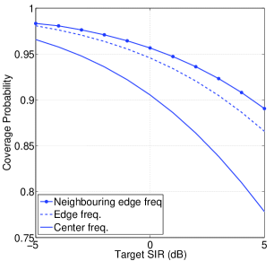
Figure 3: CP of pico user for FFR deployment in macrocell.

We would now like to analyse the impact of various FR allocation schemes in the picocell. In the next section, we propose two scheme for FR allocation and show their impact on the CP of PU and MU.

IV Proposed Frequency allocation schemes for PU

We divide the PUs into two parts: cell-centre PUs and cell-edge PUs based on the SIR threshold ($S_{tp}$). The user seeing a SIR $>S_{tp}$ is considered as cell-centre PU; else, the user is as a cell-edge PUs.

IV-A Proposed Scheme 1 for FFR

In the proposed scheme 1 (PS1), considering the reference cell of FFR deployment in Fig.1 we allocate frequency $F_{0}$ to the cell-centre PUs and frequency $F_{2}$ and $F_{3}$ to the cell-edge PUs. In other words, the centre frequency of macrocell will be used by cell-centre PUs, and neighbouring macro cell-edge frequencies would be used by cell-edge PUs. Now, we derive the CP of PUs when PS$1$ is used in the picocell. The CP of a typical PU, when PU uses PS$1$ is given by

$$\textstyle P_{ps1}=\int\limits_{0}^{R}\left(P[\eta_{p}(r)>T|\eta_{p}(r)>S_{tp}]P[\eta_{p}(r)>S_{tp}]+P[{\eta}^{e}_{p}(r)>T|\eta_{p}(r)<S_{tp}]P[\eta_{p}(r)<S_{tp}]\right)\frac{2r}{R^{2}}\text{d}r$$ (12)

where ${\eta}^{e}_{p}(r)$ denotes the SIR experienced by PU when PU uses neighbouring cell-edge frequencies. Here, the first term denotes the CP due to cell-centre PUs, and the second term denotes the CP due to cell-edge PUs. Note that

$$P[\eta_{p}(r)>T|\eta_{p}(r)>S_{t}]P[\eta_{p}(r)>S_{t}]\stackrel{{\scriptstyle(g)}}{{=}}P[\eta_{p}(r)>\max\{S_{tp},T\}]$$ (13)

Here $(g)$ follows from the Bayes’ rule. Since fading power is assumed to be independent across the sub-bands, one obtains,

$$P[{\eta}^{e}_{p}(r)>T|\eta_{p}(r)<S_{tp}]=P[{\eta}^{e}_{p}(r)>T]$$ (14)

Using (13) and (14), $P_{Ps1}$ can be simplified as

$$P_{ps1}=\int\limits_{0}^{R}(P[\eta_{p}(r)>\max\{S_{tp},T\}]+P[{\eta}^{e}_{p}(r)>T]P[\eta_{p}(r)<S_{tp}])\frac{2r}{R^{2}}\text{d}r$$ (15)

$P[\eta_{p}(r)>T]$ has been derived in Lemma $1$, and is given by

$$P[\eta_{p}(r)>T]=\exp(-\pi r^{2}T^{2/\alpha}K(r))$$ (16)

where $K(r)$ is defined in (5). Also, $P[{\eta}^{e}_{p}(r)>T]$ is derived in Lemma $2$ and is given by

$$\textstyle P[{\eta}^{e}_{p}(r)>T]=\exp\{-\pi r^{2}(T)^{2/\alpha}C(L_{p}(r),\alpha)\lambda_{p}\}\mathbb{E}_{q}\left[\exp\{-\pi r^{2}\left(\frac{TP_{m}}{P_{p}}\right)^{2/\alpha}C(L_{m}(r,q),\alpha)\frac{\lambda_{m}}{\delta}\}\right]$$ (17)

Using (15), (16) and (17), $P_{ps1}$ can be evaluated.

IV-B Proposed Scheme 2 for FFR

In the second scheme (PS2), again with reference to the FFR as depicted in Fig. 1, we allocate frequency $F_{1}$ to the cell-centre PUs and frequency $F_{2}$ and $F_{3}$ to the cell-edge PUs. Thus, the edge frequency of macrocell will be used by cell-centre PUs and the neighbouring cell-edge frequencies would be used by cell-edge PUs. The CP of PS$2$ is directly follows from the CP of PS$1$ derived in the previous section except for the fact that instead of $K(r)$ in (16), $\hat{K}(r)$ (given in (7)) will be used since the edge frequency of FFR is used by the cell-centre PU.

Now, our focus will be on the CP of cell-edge MUs when PS$2$ is used in picocell. First we derive the CP of cell-edge MUs when macrocell uses FFR and there is no picocell. Although it is already been derived in [18, Theorem 2], it will be seen that our derived expression is simpler to evaluate, and matches with the simulation result. The CP of cell-edge MUs at a distance $r$ from the BS is given by

$$P_{ed}(r)=P[\hat{\eta}(r)>T|\eta(r)<S_{tm}].$$ (18)

Here $\eta(r)$ denote the SIR experienced by MU when it uses centre frequency, and $\hat{\eta}(r)$ denotes the SIR experienced by MU when it uses cell-edge frequency and the picocell is absent. Since fading power is assumed to be independent across the sub-bands,

$$P[\hat{\eta}(r)>T|\eta(r)<S_{tm}]=P[\hat{\eta}(r)>T]$$ (19)

The CP of a typical cell-edge MU is then given by

$$P_{ed}=\frac{\int\limits_{0}^{\infty}P[\hat{\eta}(r)>T|\eta(r)<S_{tm}]P[\eta(r)<S_{tm}]f_{R}(r)\text{d}r}{\int\limits_{0}^{\infty}P[\eta(r)<S_{tm}]f_{R}(r)\text{d}r}$$ (20)

where $f_{R}(r)$ is the pdf of $r$ (which is the distance between user and the nearest MBS), and is given by [17]

$$f_{r}(R)=2\pi\lambda re^{-\lambda\pi r^{2}},r>0$$ (21)

Using (19), $P_{ed}$ in (20) can be simplified as

$$P_{ed}=\frac{\int\limits_{0}^{\infty}P[\hat{\eta}(r)>T]P[\eta(r)<S_{tm}]f_{R}(r)\text{d}r}{\int\limits_{0}^{\infty}P[\eta(r)<S_{tm}]f_{R}(r)\text{d}r}$$ (22)

In [17], it has been shown that

$$P[\eta(r)>T]=e^{-\pi\lambda r^{2}\rho(T,1)}\text{ and }P[\hat{\eta}(r)>T]=e^{-\pi\lambda r^{2}\rho(T,\delta)}$$ (23)

where

$$\textstyle\rho(T,\delta)=\frac{T^{\frac{2}{\alpha}}}{\delta}\int\limits_{T^{-2/\alpha}}^{\infty}\frac{1}{1+u^{\alpha/2}}\text{d}u=\frac{2T}{\delta(\alpha-2)}{}_{2}F_{1}(1,\frac{\alpha-2}{\alpha},2-\frac{2}{\alpha},-T)$$

Thus, $P_{ed}$ can be further simplified to

$$P_{ed}=\frac{2\pi\lambda_{m}\int\limits_{0}^{\infty}re^{-\pi\lambda_{m}r^{2}}e^{-\pi\lambda_{m}r^{2}\rho(T,\delta)}(1-e^{-\pi\lambda_{m}r^{2}\rho(S_{tm},1)})\text{d}r}{2\pi\lambda_{m}\int\limits_{0}^{\infty}re^{-\pi\lambda_{m}r^{2}}(1-e^{-\pi\lambda_{m}r^{2}\rho(S_{tm},1)})\text{d}r}$$ (24)

Solving the integrals, $P_{ed}$ can be rewritten as

$$P_{ed}=\frac{\frac{1}{1+\rho(T,\delta)}-\frac{1}{1+\rho(T,\delta)+\rho(S_{tm},1)}}{1-\frac{1}{1+\rho(S_{tm},1)}}=\frac{1+\rho(S_{tm},1)}{(1+\rho(T,\delta))(1+\rho(T,\delta)+\rho(S_{tm},1))}$$ (25)

Now, we derive the CP of cell-edge MUs when PS$2$ is used in the picocell, and the macrocell employs FFR. The CP of cell-edge MUs at a distance $r$ from the BS is given by

$$P_{ed,ps2}(r)=P[\hat{\eta}_{m}(r)>T|\eta_{m}(r)<S_{tm}]$$ (26)

and $\hat{\eta}_{m}(r)$ denotes the SIR experienced by MU when it uses FR$\delta$, and the picocell uses the PS$2$. Since fading power is assumed to be independent, we have

$$P[\hat{\eta}_{m}(r)>T|\eta_{m}(r)<S_{tm}]=P[\hat{\eta}_{m}(r)>T]$$ (27)

The CP of a typical cell-edge MU is then given by

$$P_{ed,ps2}=\frac{\int\limits_{0}^{\infty}P[\hat{\eta}_{m}(r)>T]P[\eta_{m}(r)<S_{tm}]f_{R}(r)\text{d}r}{\int\limits_{0}^{\infty}P[\eta_{m}(r)<S_{tm}]f_{R}(r)\text{d}r}$$ (28)

Note that

$$P[\hat{\eta}_{m}(r)>T]=\mathbb{P}\left[\frac{g_{m}r^{-\alpha}}{\hat{I}_{\phi\setminus M_{0}}+\frac{P_{p}}{P_{m}}I_{\psi}}>T\bigg{|}r\right],$$

$$=\mathbb{P}\left[g_{m}>Tr^{\alpha}\left(\hat{I}_{\phi\setminus M_{0}}+\frac{P_{p}}{P_{m}}I_{\psi}\right)\right]=\mathcal{L}_{\hat{I}_{\phi\setminus M_{0}}}(Tr^{\alpha})\mathcal{L_{I_{\psi}}}\left(\frac{P_{p}}{P_{m}}Tr^{\alpha}\right),$$ (29)

We know from (23) that $\mathcal{L}_{\hat{I}_{\phi\setminus M_{0}}}(s)=P[\hat{\eta}(r)>T]=e^{-\pi\lambda_{m}r^{2}\rho(T,\delta)}$, and

$$\mathcal{L}_{I_{\psi}}(s)=\mathbb{E}_{\psi,g_{j}}\left[\exp\left(-s\sum_{j\in\psi}g_{j}r_{j}^{-\alpha}\right)\right]$$

$$\stackrel{{\scriptstyle(h)}}{{=}} \exp\left(-2\pi\lambda_{p}\int_{R}^{\infty}\frac{sx^{-\alpha}}{1+sx^{-\alpha}}x\text{d}x\right)$$

$$= \exp\left(-2\pi\lambda_{p}s^{\frac{2}{\alpha}}\int_{L_{m}(r)}^{\infty}\frac{t}{1+t^{\alpha}}\text{d}t\right)$$

$$= \exp\{-\pi s^{2/\alpha}C(L_{m}(r),\alpha)\lambda_{p}\}$$ (31)

where $L_{m}(r)=\frac{R}{r}(T)^{-\frac{1}{\alpha}}$. The lower limit of the integral in $(h)$ is $R$ because of the fact that all the interfering PBS are at least a distance greater than $R$. Thus, the CP of a typical cell-edge MU is given by

$$P_{ed,ps2}=\frac{2\pi\lambda_{m}\int\limits_{0}^{\infty}e^{-\pi\lambda_{m}r^{2}}e^{-\pi\lambda_{m}r^{2}\rho(T,\delta)}\exp\{-\pi(\frac{P_{p}T}{P_{m}})^{\frac{2}{\alpha}}r^{2}C(L_{m}(r),\alpha)\lambda_{p}\}(1-e^{-\pi\lambda_{m}r^{2}\rho(S_{tm},1)})\text{d}r}{1-\frac{1}{1+\rho(S_{tm},1)}}$$ (32)

We now derive the CP of cell-centre MU. The CP of cell-centre MU without picocell is given in [18, Theorem 3]. The CP of cell-centre MU when PS$1$ is used in the picocell is given by

$$P_{cen,ps1}=\frac{\int\limits_{0}^{\infty}P[\eta_{m}(r)>\max\{S_{tm},T\}]f_{R}(r)}{\int\limits_{0}^{\infty}P[\eta_{m}(r)>T]f_{R}(r)}$$ (33)

Note that

$$P[\eta_{m}(r)>T]=\mathbb{P}\left[\frac{g_{m}r^{-\alpha}}{I_{\phi\setminus M_{0}}+\frac{P_{p}}{P_{m}}I_{\psi}}>T\right]=\mathcal{L}_{I_{\phi\setminus M_{0}}}(Tr^{\alpha})\mathcal{L_{I_{\psi}}}(\frac{P_{p}}{P_{m}}Tr^{\alpha}),$$

We know from (31), $\mathcal{L_{I_{\psi}}}(\frac{P_{p}}{P_{m}}Tr^{\alpha})=\exp\{-\pi(\frac{P_{p}T}{P_{m}})^{\frac{2}{\alpha}}r^{2}C(L_{p}(r),\alpha)\lambda_{p}\}$ and $\mathcal{L}_{I_{\phi\setminus M_{0}}}(Tr^{\alpha})=P[\eta(r)>T]=e^{-\pi\lambda_{m}r^{2}\rho(T,1)}$ from (23), and hence CP of cell-centre MU can be derived. The CP of cell-centre MU does not change when PS$2$ is used in the picocell, since PS$2$ does not use centre frequency resources.

IV-C Average Rate

In this subsection, we derive average rate for both the schemes. The average rate $R$ can be written as

$$R=E[\ln(1+\text{SIR})]=\int\limits_{t>0}P[\ln(1+\text{SIR})>t]\text{d}t.$$

Using the fact that $\ln(1+\text{SIR})$ is a monotonic increasing function for SIR, one obtains,

$$R=\int\limits_{t>0}P[\text{SIR}>e^{t}-1]\text{d}t.$$ (34)

This is equivalent to computing CP for $T=e^{t}-1$ and integrating it over $t$. The CP for the PS$1$ is given in (15), and thus the average rate of PU in PS$1$ is given by

$$R_{ps1}=\int\limits_{t>0}\left(\int\limits_{0}^{R}(P[\eta_{p}(r)>\max\{S_{tp},e^{t}-1\}]+P[\hat{\eta}_{p}(r)>e^{t}-1]P[\eta_{p}(r)<S_{tp}])\frac{2r}{R^{2}}\text{d}r\right)\text{d}t$$ (35)

where $P[\eta_{p}(r)>T]$ and $P[\hat{\eta}_{p}(r)>T]$ are given in (16) and (17), respectively. Similarly, the average rate of PU in PS$2$ can be derived. In order to choose $S_{tp}$, we define the sub-bands allocation to the MU and PU. Here, based on the SIR threshold sub-bands allocation can be done [22] [18]. In other words,

$$N_{c}=P[\eta_{m}>S_{tm}]N_{t}\text{ and }N_{e}=\frac{N_{t}-N_{c}}{3}$$ (36)

where $N_{t}=F_{0}+F_{1}+F_{2}+F_{3}$, $N_{c}=F_{0}$, and $N_{e}=F_{1}=F_{2}=F_{3}$, denote the total sub-bands, centre sub-bands, and the edge sub-bands, respectively. Since PS$1$ allocates the centre frequency band of the macrocell to the cell-centre PUs, $S_{tp}$ for the PS$1$ can be chosen such that

$$P_{f,c}(S_{tp})=\frac{N_{c}}{N_{t}}$$ (37)

Here, $P_{f,c}(S_{tp})$ is derived in Lemma $1$, Similarly, the $S_{tp}$ for the PS$2$ can be chosen such that

$$P_{f,e}(S_{tp})=\frac{N_{e}}{N_{t}},$$ (38)

where $P_{f,e}(S_{tp})$ is given by (6). To compare the average rate for both the schemes, we define a normalized average rate which is average rate times the fraction of the total sub-bands used in that particular scheme. In other words, the normalized average rate of PS$1$ is $\frac{R_{ps1}(F_{0}+F_{2}+F_{3})}{N_{t}}$, and similarly the normalized average rate of PS$2$ is $\frac{R_{ps2}(F_{1}+F_{2}+F_{3})}{N_{t}}$.

IV-D Analysis and Comparison of PS1 and PS2 for FFR

In this subsection, we analyse the performance of PS$1$ and PS$2$ and compare both these schemes. Fig. 4 shows the CP of PU when picocell uses either PS$1$ or PS$2$, and it also plots the CP of the conventional scheme. Here again we take $P_{m}=46$dBm, $P_{p}=30$dBm, $\lambda_{m}=0.385/Km^{2}$, $\lambda_{p}=1.155/Km^{2}$ $\delta=3$, and $R=200$ meters It can be seen that PS$2$ provides better CP than PS$1$, and both have a significantly better performance when compared to the conventional scheme.

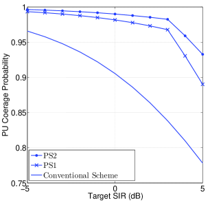
Figure 4: CP of pico user for the proposed schemes. Here $S_{tp}=3$dB and $\alpha=4$.

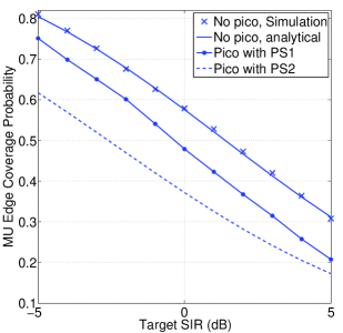
Figure 5: CP of cell-edge MUs where picocell are using different proposed schemes. Here $S_{tm}=0$dB and $\alpha=3.2$.

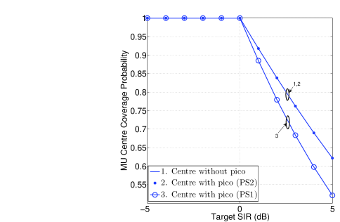
Figure 6: CP of cell-centre MUs where picocell uses different proposed schemes. Here $S_{tm}=0$dB and $\alpha=3.2$.

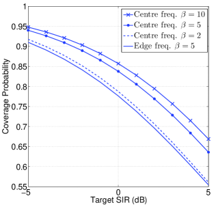
Figure 8: CP of pico user for SFR deployment in macrocell.

We will now study the impact of the proposed schemes on the CP of the MUs. Fig. 8 shows the CP of cell-edge MUs for three cases: $(i)$ when there is no picocell, $(ii)$ when picocell uses PS$1$, and $(iii)$ when picocell use PS$2$. Here, the CP of cell-edge MU when picocell uses PS$1$ is plotted using simulation. It can be observed that the CP of cell-edge MU is lowest when PS$2$ is used in the picocell. The CP of cell-edge MU when there is no picocell is highest followed by when PS$1$ is used in the picocell. Fig. 6 show the impact of proposed schemes on the centre CP. The CP of cell-centre degrades when picocell uses PS$1$. However, there is no impact of PS$2$ on the CP of the cell-centre MU, since PS$2$ does not use cell-centre resources at the picocells. Fig. 7 plots the normalized average rate with respect to SIR threshold of macrocell. It can be seen that as $S_{tm}$ increases, centre frequency of macrocell ($N_{c}$) decreases, i.e., the sub-bands of picocell for PS$1$ decreases and the sub-bands of picocell for PS$2$ increases. Hence, the normalized average rate of PS$1$ decreases and the normalized average rate of PS$2$ increases.

Based on the above results, we see that in FFR deployments, both PS$1$ and PS$2$ have an advantage over the conventional scheme, but neither of them is uniformly better than the other. Then, the question arises which of these two schemes should the operator use in the picocell? We provide following guidelines that could help this choice:

1. Depending on the SIR threshold chosen for the macrocell, PS$1$ or PS$2$ can be selected.

2. The proposed schemes allocation could also depend on the MUs around the picocell. If cell-edge MUs around one particular picocell are higher then that picocell should use the PS$2$ rather PS$1$ and vice versa.

3. It could also depend on the location of picocell with respect to nearest macrocell. It is seen by simulation that as picocell location moves towards the edge of nearest macrocell, the gap between the CP of PU corresponding to PS$1$ and PS$2$ increases. In other words, the CP of PU corresponding to PS$2$ is much higher than the CP of PU corresponding to PS$1$ when picocell location is at the edge of macrocell. Hence, depending on the location of picocell, proposed scheme selection can be made.

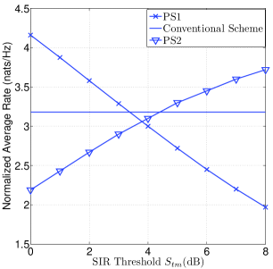
Figure 7: Normalized average rate of PU. Here $\alpha=4$.

V Frequency Allocation for PU When MBS Employ SFR

In this section, we first derive the CP for PU when MBS employ SFR. In order to calculate the CP of PU when MBS uses SFR, we divide the interference due to MBSs into two parts: interference due to the nearest MBS, and the interference due to all the remaining MBSs. The effective interference power due to all remaining MBSs is denoted by $\eta P_{m}$, where as in [18], $\eta=\frac{\delta-1+\beta}{\delta}$.

Lemma 3.

The CP of a typical PU, using the centre frequency resources band $F_{2}$ or $F_{3}$ of the SFR for an interference limited scenario is given by

$$\textstyle P_{s,c}(T)=\int_{r>0}^{R}\frac{2r}{R^{2}}\exp\{-\pi r^{2}(T)^{2/\alpha}C(L_{p}(r),\alpha)\lambda_{p}\}\text{ }\mathbb{E}_{q}\left[\frac{P_{p}}{P_{p}+Tr^{\alpha}P_{m}{q}^{-\alpha}}e^{\{-\pi r^{2}\left(\frac{\eta TP_{m}}{P_{p}}\right)^{2/\alpha}C(L_{c}(r),\alpha)\lambda_{m}}\}\right]\mathrm{d}r$$ (39)

Proof.

CP of PU can be written as,

$$P_{s,c}=\int_{r>0}^{R}\mathbb{P}[\eta_{p}(r)>T|r]f_{r}(r)\text{d}r,$$

$$=\int_{r>0}^{R}\frac{2r}{R^{2}}\mathbb{P}\left[\frac{g_{p}r^{-\alpha}}{\eta\frac{P_{m}}{P_{p}}I_{\phi\setminus M_{0}}+I_{\psi\setminus P_{0}}+\frac{P_{m}}{P_{p}}{q}^{-\alpha}{h_{0}}}>T|r\right]\text{d}r,$$

$$=\int_{r>0}^{R}\frac{2r}{R^{2}}\mathcal{L}_{I_{\phi\setminus M_{0}}}(Tr^{\alpha}\eta\frac{P_{m}}{P_{p}})\mathcal{L}_{I_{\psi\setminus P_{0}}}(Tr^{\alpha})\exp\{-Tr^{\alpha}\frac{P_{m}}{P_{p}}{q}^{-\alpha}{h_{0}}\}\text{d}r.$$ (40)

Here the first term $\mathcal{L}_{I_{\phi\setminus M_{0}}}(Tr^{\alpha}\eta\frac{P_{m}}{P_{p}})$ is due to interference from all the MBS except the nearest MBS, and the second term $\mathcal{L}_{I_{\psi\setminus P_{0}}}(Tr^{\alpha})$ is due to interference from all the picocell except the serving picocell, and third term $\exp\{-Tr^{\alpha}\frac{P_{m}}{P_{p}}{q}^{-\alpha}{h_{0}}\}$ is due to interference from the nearest MBS. Where, $h_{0}$ is the fading power gain from the nearest MBS and $h_{0}\sim\exp(1)$ hence one obtains,

$$\mathbb{E}_{h_{0}}[\exp\{-Tr^{\alpha}\frac{P_{m}}{P_{p}}{q}^{-\alpha}{h_{0}}\}]=\frac{P_{p}}{P_{p}+Tr^{\alpha}P_{m}{q}^{-\alpha}}$$ (41)

$\mathcal{L}_{I_{\phi\setminus M_{0}}}(s)$ is given in (11) and $\mathcal{L}_{I_{\psi\setminus P_{0}}}(Tr^{\alpha})$ has been derived in the Appendix (please see Eq. (44)). Hence using (11) and (44), Eq. (40) can be simplified to obtain (39). ∎

Now, the case when PU uses the edge frequency resources band $F_{1}$ of the SFR will be analysed. The CP of PU in this case directly follows from an application of Lemma $3$ except for the fact that the edge frequency uses $\beta$ times higher power than the centre frequency. Therefore, interference due to the nearest MBS will be $(1+\beta Tr^{\alpha}\frac{P_{m}}{P_{p}}{q}^{-\alpha})^{-1}$ instead of $(1+Tr^{\alpha}\frac{P_{m}}{P_{p}}{q}^{-\alpha})^{-1}$. Hence, the CP of a typical PU, using the edge frequency resources band $F_{1}$ of the SFR for an interference limited scenario is given by an expression identical to (39), but with $(1+Tr^{\alpha}\frac{P_{m}}{P_{p}}{q}^{-\alpha})^{-1}$ within the expectation replaced by $(1+\beta Tr^{\alpha}\frac{P_{m}}{P_{p}}{q}^{-\alpha})^{-1}$.

The impact of SFR on the CP of PU is plotted in Fig. 4. Here again we take $\delta=3$, $\alpha=3.2$, and $R=200$ meters. This result shows that the edge frequency resources give the lowest CP among all the frequency resources in the SFR scheme. Centre frequency resources provide a higher coverage than the edge frequency resources because of the fact that they use $\beta$ times less power for the nearest MBS. Now, as we increase $\beta$, the power on the centre frequency resources decreases with respect to edge frequency resources, and this results in a higher coverage. Hence, centre frequency resources in SFR should only be used by the picocell.

VI Conclusions

This work considered FFR and SFR deployments for the macrocell, and provided the CP and rate of a PU by assuming a fixed size picocell. We proposed two schemes for the picocell when the macrocell employs FFR. The CP and rate of proposed schemes were derived, and it was shown that the proposed schemes outperforms the conventional scheme. The impact of the proposed schemes on the CP of MU was also discussed. Finally, the spectrum allocation in picocell was briefly discussed when the macrocell employed SFR. Future work could consider the effect of range expansion (or picocell strength bias) [19], on the performance of the proposed schemes. Further extension of this work could include the effect of correlation among the interferers [20]. Another important extension of this work is to analyse the performance of the proposed schemes in an uplink cellular network [21].

Proof of Lemma 1

Given that the typical PU is at distance $r$ from the PBS, the CP averaged over the picocell area is given by

$$P_{f,c}(T)=\mathbb{E}_{r}[\mathbb{P}[\text{SIR}>T|r]]=\int_{r>0}^{R}\mathbb{P}[\eta_{p}(r)>T|r]f_{r}(r)\text{d}r,$$

$$=\int_{r>0}^{R}\frac{2r}{R^{2}}\mathbb{P}\left[\frac{g_{p}r^{-\alpha}}{\frac{P_{m}}{P_{p}}I_{\phi}+I_{\psi\setminus P_{0}}}>T|r\right]\text{d}r,$$

$$= \int_{r>0}^{R}\frac{2r}{R^{2}}\mathbb{P}[g_{m}>Tr^{\alpha}(\frac{P_{m}}{P_{p}}I_{\phi}+I_{\psi\setminus P_{0}})|r]\text{d}r,$$ (42)

$$\stackrel{{\scriptstyle(a)}}{{=}} \int_{r>0}^{R}\frac{2r}{R^{2}}\mathcal{L_{I_{\phi}}}(Tr^{\alpha}\frac{P_{m}}{P_{p}})\mathcal{L}_{I_{\psi\setminus P_{0}}}(Tr^{\alpha})\text{d}r,$$

where $I_{\phi}=\sum\limits_{i\in\phi}{d_{i}}^{-\alpha}{h_{i}},$ $I_{\psi\setminus P_{0}}=\sum\limits_{j\in(\psi\setminus P_{0})}{r_{j}}^{-\alpha}{g_{j}}$. Here $(a)$ follows from the fact that $g_{m}\sim\exp(1)$. $\mathcal{L_{I_{\phi}}}(s)$ and $\mathcal{L}_{I_{\psi\setminus P_{0}}}(s)$ are the Laplace transforms of the random variables $I_{\phi}$ and $I_{\psi}$, respectively, evaluated at $s$. Thus,

$$\mathcal{L}_{I_{\psi\setminus P_{0}}}(s)=\mathbb{E}_{{\psi\setminus P_{0}},g_{j}}[\exp(-s\sum_{j\in\psi\setminus P_{0}}g_{j}r_{j}^{-\alpha})]$$

$$\stackrel{{\scriptstyle(b)}}{{=}} \exp\left(-2\pi\lambda_{p}\int_{R+R_{g}^{(p)}-r}^{\infty}\frac{sx^{-\alpha}}{1+sx^{-\alpha}}x\text{d}x\right)$$

$$\stackrel{{\scriptstyle(c)}}{{=}} \exp\left(-2\pi\lambda_{p}s^{\frac{2}{\alpha}}\int_{L_{p}(r)}^{\infty}\frac{t}{1+t^{\alpha}}\text{d}t\right)$$

$$\stackrel{{\scriptstyle(d)}}{{=}} \exp\{-\pi s^{2/\alpha}C(L_{p}(r),\alpha)\lambda_{p}\}$$ (44)

$$L_{p}(r)=\frac{R+R_{g}^{(p)}-r}{r}(T)^{-\frac{1}{\alpha}},\text{ and }C(L_{p}(r),\alpha)=\frac{{}_{2}F_{1}(1,\frac{\alpha-2}{\alpha},2-\frac{2}{\alpha},-\{L_{p}(r)\}^{\alpha})}{\alpha-2}\{L_{p}(r)\}^{2-\alpha}.$$ (45)

Here, $(b)$ follows from the fact that $g_{j}\sim\exp(1)$ and probability generating functional (PGFL) [23] of the PPP and ${}_{2}F_{1}(a,b,c,z)$ represents the Gauss hypergeometric function. The lower limit of the integral in $(b)$ is $R+R_{g}^{(p)}-r$ because of the fact that all the interfering base stations are at least a distance greater than $R+R_{g}^{(p)}-r$. Using a change of variable $t=s^{-\frac{1}{\alpha}}x$, $(c)$ can be followed and $(d)$ follows after some algebraic manipulation. In a similar fashion,

$$\mathcal{L}_{I_{\phi}}(s)=\exp\{-\pi s^{2/\alpha}C(L_{m}(r),\alpha)\lambda_{m}\}.$$ (46)

where $L_{m}(r)=\frac{R+R_{g}^{(m)}-r}{r}\left(T\frac{P_{m}}{P_{p}}\right)^{-\frac{1}{\alpha}}$. Using (44) and (46) and simplifying (42), one obtains

$$P_{f,c}(T)=\int_{r>0}^{R}\exp(-\pi r^{2}T^{2/\alpha}K(r))\frac{2r}{R^{2}}\mathrm{d}r,$$

$$\text{where }K(r)=\left(\frac{P_{m}}{P_{p}}\right)^{2/\alpha}C(L_{m}(r),\alpha)\lambda_{m}+C(L_{p}(r),\alpha)\lambda_{p}.$$

References

- [1] S. Kishore, L. Greenstein, H. Poor, and S. Schwartz, “Uplink User Capacity in a CDMA Macrocell with a Hotspot Microcell: Exact and Approximate Analyses,” IEEE Transactions on Wireless Communications, vol. 2, no. 2, pp. 364–374, 2003.
- [2] X. Wu, B. Murherjee, and D. Ghosal, “Hierarchical Architectures in the Third-Generation Cellular Network,” IEEE Wireless Communications, vol. 11, no. 3, pp. 62–71, 2004.
- [3] N. Himayat, S. Talwar, A. Rao and R. Soni, “Interference Management for 4G Cellular Standards [WIMAX/LTE UPDATE],” IEEE Communications Magazine, vol. 48, no. 8, pp. 86–92, August 2010.
- [4] D. Qin, W. Xu, and Z. Ding, “Power Control and Resource Allocation for Capacity Improvement in Picocell Downlinks,” in International Conference on Wireless Communications Signal Processing (WCSP), 2012, 2012, pp. 1–6.
- [5] H. Shimodaira, G. Tran, S. Tajima, K. Sakaguchi, K. Araki, N. Miyazaki, S. Kaneko, S. Konishi, and Y. Kishi, “Optimization of Picocell Locations and its Parameters in Heterogeneous Networks with Hotspots,” in IEEE 23rd International Symposium on Personal Indoor and Mobile Radio Communications (PIMRC), 2012, 2012, pp. 124–129.
- [6] I. Guvenc, M.-R. Jeong, I. Demirdogen, B. Kecicioglu, and F. Watanabe, “Range Expansion and Inter-Cell Interference Coordination (ICIC) for Picocell Networks,” in IEEE Vehicular Technology Conference (VTC Fall), 2011, 2011, pp. 1–6.
- [7] Y. Wang, Y. Chang, and D. Yang, “An Efficient Inter-Cell Interference Coordination Scheme in Heterogeneous Cellular Networks,” in IEEE Vehicular Technology Conference (VTC Fall), 2012, 2012, pp. 1–5.
- [8] M. Eguizabal and A. Hernandez, “Interference Management and Cell Range Expansion Analysis for LTE Picocell Deployments,” in IEEE 24th International Symposium on Personal Indoor and Mobile Radio Communications (PIMRC), 2013, 2013, pp. 1592–1597.
- [9] F. Jin, R. Zhang, and L. Hanzo, “Fractional Frequency Reuse Aided Twin-Layer Femtocell Networks: Analysis, Design and Optimization,” IEEE Transactions on Communications, vol. 61, no. 5, pp. 2074–2085, 2013.
- [10] S. Kumar and K. Giridhar, “Analytical Derivation of Reuse Pattern for Soft Frequency Reuse Based Femtocell Deployment,” in 15th International Symposium on Wireless Personal Multimedia Communications (WPMC), Sept. 2012, pp. 569–573.
- [11] J. Y. Lee, S. J. Bae, Y. M. Kwon and M. Y. Chung, “Interference Analysis for Femtocell Deployment in OFDMA Systems Based on Fractional Frequency Reuse,” IEEE Communications Letters, vol. 15, no. 4, pp. 425–427, April 2011.
- [12] H. S. Dhillon, R. K. Ganti, F. Baccelli and J. G. Andrews, “Modeling and Analysis of K-Tier Downlink Heterogeneous Cellular Networks,” IEEE Journal on Selected Areas in Communications, vol. 30, no. 3, pp. 550–560, April 2012.
- [13] T. D. Novlan, R. K. Ganti, A. Ghosh and J. G. Andrews, “Analytical Evaluation of Fractional Frequency Reuse for Heterogeneous Cellular Networks,” IEEE Transactions on Communications, vol. 60, no. 7, pp. 2029–2039, 2012.
- [14] S. Mukherjee, “Distribution of Downlink SINR in Heterogeneous Cellular Networks,” Selected Areas in Communications, IEEE Journal on, vol. 30, no. 3, pp. 575–585, 2012.
- [15] W. C. Cheung, T. Q. S. Quek and M. Kountouris, “Throughput Optimization, Spectrum Allocation, and Access Control in Two-Tier Femtocell Networks,” IEEE Journal on Selected Areas in Communications, vol. 30, no. 3, pp. 561–574, April 2012.
- [16] R. Heath, M. Kountouris, and T. Bai, “Modeling Heterogeneous Network Interference Using Poisson Point Processes,” Signal Processing, IEEE Transactions on, vol. 61, no. 16, pp. 4114–4126, 2013.
- [17] J. G. Andrews, F. Baccelli and R. K. Ganti, “A Tractable Approach to Coverage and Rate in Cellular Networks,” IEEE Transactions on Communications, vol. 59, no. 11, pp. 3122–3134, November 2011.
- [18] T. Novlan, R. Ganti, A. Ghosh, and J. Andrews, “Analytical Evaluation of Fractional Frequency Reuse for OFDMA Cellular Networks,” IEEE Transactions on Wireless Communications,, vol. 10, no. 12, pp. 4294–4305, 2011.
- [19] D. Lopez-Perez, X. Chu, and I. Guvenc, “On the Expanded Region of Picocells in Heterogeneous Networks,” IEEE Journal of Selected Topics in Signal Processing, vol. 6, no. 3, pp. 281–294, 2012.
- [20] S. Kumar and S. Kalyani, “Analysis and comparison of coverage probability in the presence of correlated nakagami-m interferers and non-identical independent nakagami-m interferers,” arXiv preprint arXiv:1401.4663, 2014.
- [21] S. Kumar and K. Giridhar, “Power control factor selection in uplink ofdma cellular networks,” arXiv preprint arXiv:1401.4657, 2014.
- [22] S. Kumar, S. Kalyani, and K. Giridhar, “Optimal thresholds for coverage and rate in ffr schemes for planned cellular networks,” arXiv preprint arXiv:1401.4662, 2014.
- [23] D. Stoyan, W. Kendall and J. Mecke, Stochastic Geometry and Its Application, 2nd ed. John Wiley and Sons, 1996.