Hemispherical Parker waves driven by thermal shear in planetary dynamos

Abstract

Planetary and stellar magnetic fields are thought to be sustained by helical motions ($\alpha$-effect) and, if present, differential rotation ($\Omega$-effect). In the Sun, the strong differential rotation in the tachocline is responsible for an efficient $\Omega$-effect creating a strong axisymmetric azimuthal magnetic field. This is a prerequisite for Parker dynamo waves that may be responsible for the solar cycle. In the liquid iron cores of terrestrial planets, the Coriolis force organizes convection into columns with a strong helical flow component. These likely dominate magnetic field generation while the $\Omega$-effect is of secondary importance. Here we use numerical simulations to show that the planetary dynamo scenario may change when the heat flux through the outer boundary is higher in one hemisphere than in the other. A hemispherical dynamo is promoted that is dominated by fierce thermal wind responsible for a strong $\Omega$-effect. As a consequence Parker dynamo waves are excited equivalent to those predicted for the Sun. They obey the same dispersion relation and propagation characteristics. We suggest that Parker waves may therefore also play a role in planetary dynamos for all scenarios where zonal flows become an important part of convective motions.

1 Introduction

The dynamo mechanism of stars and planets relies on electromagnetic induction and requires an electrically conducting medium and a complex fluid flow to maintain the magnetic fields against Ohmic decay. The liquid iron cores form the dynamo regions of terrestrial planets and the dominance of Coriolis forces guarantees sufficiently complicated convective dynamics in these fast rotating bodies. The flow is organized in convective columns parallel to the rotation axis. Secondary flows up and down these columns yield a strong helical component essential for magnetic field generation. Since this helicity associated with the local columnar motion dominates the production of the poloidal and the toroidal magnetic field contributions in many dynamo simulations they are typically classified as $\alpha^{2}$ dynamos Olson et al. (1999). The terminology goes back to the mean-field dynamo theory where an $\alpha$ stands for the creation of large-scale field by small-scale motions.

In the Sun, the differential rotation at the tachocline is the main source of large-scale axisymmetric toroidal magnetic field. Since this is called an $\Omega$-effect in mean-field dynamo theory, the solar dynamo is classified as $\alpha\Omega$ Krause and Rädler (1980). A powerful $\Omega$-effect may be the reason for the oscillatory nature of the solar magnetic field which has not been observed in planetary dynamos. Strong axisymmetric toroidal fields are a prerequisite for Parker dynamo waves Parker (1955) which seem to mimic the general oscillating behaviour to a large extent.

In the framework of the classical mean-field model of an axisymmetric $\alpha\Omega$-dynamo Parker (1955), Parker waves are purely magnetic oscillations between the poloidal and toroidal mean magnetic field components. Poloidal field is exclusively created by the $\alpha$-effect as the parametrization of the nonaxisymmetric helical flows, whereas the azimuthal toroidal field is induced by the axisymmetric differential rotation or the $\Omega$-effect Tobias and Weiss (2007).

The minimum frequency of these waves is simply the inverse of the magnetic diffusion time $\tau_{\lambda}=D^{2}/\lambda$ Rüdiger and Hollerbach (2004). Assuming a turbulent bulk magnetic diffusivity of $\lambda=10^{8}\,\mathrm{m^{2}/s}$ for the solar convective shell of thickness $D=2\times 10^{8}\,\mathrm{m}$, the magnetic diffusion time is $\tau_{\lambda}=12.7\,\mathrm{yr}$ and matches the time scale of a solar cycle ($22\,\mathrm{yr}$) reasonably well.

Parker waves are typically associated with dynamo models where stress free flow boundary conditions allow strong zonal winds to arise. These guarantee a strong $\Omega$-effect and thereby promote Parker waves. Parker-wave like oscillation in combination with a hemispherical magnetic field have previously been reported by Grote and Busse (2000). Because of the stress free flow boundary conditions and the fixed temperature conditions their model also seems more appropriate for a stellar application.

Here we report that Parker waves also appear in simulations of planetary dynamos when lateral variations in the heat flux through the outer boundary lead to fierce zonal winds and thus strong $\Omega$-effects. More specifically, we consider a model for the ceased ancient Martian dynamo which left its trace in form of a remanent crustal magnetization. The magnetization shows a hemispherical distribution with much higher values in the southern than in the northern hemisphere Acuña et al. (1999). Recent studies aim at explaining this pattern with the fact that the dynamo itself produced a hemispherical field Stanley et al. (2008); Dietrich and Wicht (2013). Such dynamos are promoted when the heat flux through the southern core-mantle boundary is significantly larger than that through the northern. In terrestrial planets, the core-mantle-boundary heat flux is determined by the thermal mantle structure which develops on much slower time scales than core convection. A major impact in the northern hemisphere or a large-scale mantle convection pattern are two alternative scenarios causing a north/south heat flux asymmetry Stanley et al. (2008).

Since the southern hemisphere of the core is cooled more efficiently than its northern counterpart, a latitudinal temperature gradient develops that drives fierce thermal winds. When the heat flux asymmetry is large enough these winds clearly dominate the flow. The dynamo then changes from an $\alpha^{2}$ to an $\alpha\Omega$ type and shows wave-like behaviour reminiscent of Parker waves Dietrich and Wicht (2013). Here we analyse a suite of hemispherical dynamo simulations to determine when these waves arise. By showing that the frequency of the waves follows the theoretical dispersion relation based on mean-field theory we clearly establish their Parker wave nature.

2 Model

The full MHD dynamo problem is defined by the equations for conservation of momentum, for the evolution of the superadiabatic temperature perturbation $T$ and for the evolution of the magnetic field $\bf{B}$. For a rotating spherical shell and assuming the Boussinesq-approximation these equations read

$$\frac{E}{Pm}\left(\frac{\partial\bf{u}}{\partial t}+\bf{u}\cdot\bf{\nabla}\bf{u}\right)-E\bf{\nabla}^{2}\bf{u}=-\bf{\nabla}\Pi$$ (1)

$$\hskip 28.45274pt-2\hat{\bf{z}}\times\bf{u}+Ra_{q}^{\star}Pm\frac{\bf{r}}{r_{o}}T+(\bf{\nabla}\times\bf{B})\times\bf{B}\,$$

$$\frac{\partial T}{\partial t}+\bf{u}\cdot\bf{\nabla}T=\frac{Pm}{Pr}\nabla^{2}T+\epsilon$$ (2)

$$\frac{\partial\bf{B}}{\partial t}-\bf{\nabla}\times\left(\bf{u}\times\bf{B}\right)=\bf{\nabla}^{2}\bf{B}\ .$$ (3)

Here $\bf{u}$ is the velocity, $\Pi$ is the non-hydrostatic pressure, $\epsilon$ a homogeneous heat source density that models the cooling of the planet, and $\hat{\bf{z}}$ the unit vector parallel to the axis of rotation. Above equations have been made dimensionless using the magnetic diffusion time $D^{2}/\lambda$ as a time scale and the shell thickness $D=r_{o}-r_{i}$ as a length scale, where $r_{o}$ and $r_{i}$ are the outer and inner shell radii, respectively, and $\lambda$ is the magnetic diffusivity. The magnetic scale is $(\mu\lambda\rho\Omega)^{1/2}$ with $\mu$ the magnetic permeability, $\rho$ the mean density, and $\Omega$ the rotation rate.

The dimensionless control parameters are the Ekman number $E=\nu/\Omega D^{2}$, a measure of the ratio of viscous to Coriolis force, the modified flux based Rayleigh number $Ra_{q}^{\star}=Ra_{q}E/Pr=\beta q_{o}g_{o}D^{2}/\rho c_{p}\nu\kappa\Omega$, the hydrodynamic Prandtl $Pr=\nu/\kappa$ and magnetic Prandtl number $Pm=\nu/\lambda$. Here, $\kappa$ is the thermal diffusivity, $\nu$ the kinematic viscosity, $g_{o}$ the gravity at the outer boundary, $\beta$ the thermal expansivity, $\rho$ the density, $c_{p}$ the specific heat and $q_{0}$ the superadiabatic outer boundary heat flux.

The choice of rigid flow boundaries and an electrically insulating mantle and inner core is motivated by the application to terrestrial planets Dietrich and Wicht (2013). To more specifically model the ancient Martian dynamo where likely no inner core was present we drive convection by homogeneously distributed heat sources $\epsilon$ which is equivalent to secular cooling. For numerical reasons, we kept an inner core with an aspect ratio of $r_{i}/r_{o}=0.35$ in our simulations but set the inner boundary heat flux to zero to minimize its impact. The total heating $V\epsilon$ is balanced by the total heat loss through the outer boundary $4\pi r_{o}^{2}q_{0}$, where $V$ is the volume of the outer core and $q_{0}$ is the mean heat flux density through the outer boundary. Further to modify the heat escape out of the spherical shell we assume a cosine variation of the outer boundary heat flux like

$$q=q_{0}(1-q^{\star}\cos{}\vartheta)\;\;,$$ (4)

where $\vartheta$ is the colatitude and $q^{\star}$ the relative variation amplitude. Thus setup was first proposed by Stanley et al. (2008).

For the bulk of the numerical results the nondimensional parameters are fixed to $E=10^{-4},Ra_{q}=4.1\times 10^{7},Pm=2,Pr=1$ and we gradually increase $q^{\star}$ up to $3$. All simulations were performed with the MagIC3 code Wicht (2002) using a resolution $N_{r}\times N_{\varphi}\times N_{\vartheta}$ of maximal $65\times 320\times 160$. After equilibration each model ran for at least one (typically more) magnetic diffusion time. We avoided the usage of azimuthal symmetries or hyperdiffusion to speed up the simulations.

2.1 Mean-field theory

Mean-field theory focusses on solving the large-scale induction equation by parameterizing the effects of small-scale magnetic field and flow. Using appropriate averaging techniques, magnetic field and flow are both separated into a mean or large-scale contribution, denoted by overbars, and fluctuating or small-scale contribution, denoted by primes:

$$\bf{u}=\overline{\bf{u}}+\bf{u}^{\prime},\,\bf{B}=\overline{\bf{B}}+\bf{B}^{\prime}$$ (5)

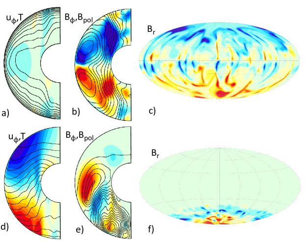
Figure 1: Comparison of the homogeneous reference case (upper row) and a hemispherically modified dynamo (lower row). The left plots (a and d) show the colour coded zonal flow with the axisymmetric temperature as contours, the middle plot characterizes the azimuthal field in colour and the poloidal field lines as contours (b and e). The right plots display the radial field at the outer boundary (c and f). All plots are snapshots.

For our purpose we use azimuthal averages so that $\overline{\bf{u}}$ and $\overline{\bf{B}}$ are the axisymmetric and $\bf{u}^{\prime}$ and $\bf{B}^{\prime}$ are the non-axisymmetric contributions. In the induction equation for the mean field $\overline{\bf{B}}$, we reduce the action of $\overline{\bf{u}}$ to the $\Omega$-effect since other contributions are likely much smaller. The action of the fluctuating flow $\bf{u}^{\prime}$ is parameterized by the $\alpha$-effect, assuming homogeneous turbulence Krause and Rädler (1980). Following recent studies, such as Busse and Simitev (2006) and Schrinner et al. (2011), we investigate axisymmetric $\alpha\Omega$ and $\alpha^{2}\Omega$-dynamos responsible for creating an axisymmetric mean field $\overline{\bf{B}}=B\bf{e}_{\varphi}+\bf{\nabla}\times A\bf{e}_{\varphi}$, with toroidal vector potential $A$, representing the poloidal field, and toroidal field $B$:

$$\frac{\partial A}{\partial t} =\alpha B+\Delta A$$ (6)

$$\frac{\partial B}{\partial t} =-\alpha\Delta A+\frac{\partial\overline{u}}{\partial x_{2}}\frac{\partial A}{\partial x_{3}}+\Delta B\ .$$ (7)

For remaining consistent with previous formulations Schrinner et al. (2011), we use cartesian coordinates $x_{1},x_{2},x_{3}$ corresponding to the spherical $\varphi,\vartheta,r$, respectively. As a solution for this system of equations, Parker Parker (1955) suggested propagating plane dynamo waves obeying the following dispersion relations for the frequency $\nu$ in the $\alpha\Omega$ and $\alpha^{2}\Omega$ limit:

$$\nu_{\alpha\Omega} =\sqrt{\frac{\alpha}{2}}\sqrt{k_{3}\frac{\partial\overline{u}}{\partial x_{2}}}\ ,$$ (8)

$$\nu_{\alpha^{2}\Omega} =\sqrt{\frac{\alpha}{2}}\sqrt{\sqrt{\left(\alpha k^{2}\right)^{2}+\left(k_{3}\frac{\partial\overline{u}}{\partial x_{2}}\right)^{2}}-\alpha k^{2}}\ ,$$ (9)

The total wave number $k$ with $k^{2}=k_{2}^{2}+k_{3}^{2}$ has the two contributions $k_{2}$ and $k_{3}$ in the $\vartheta$- and $r$-direction, respectively.

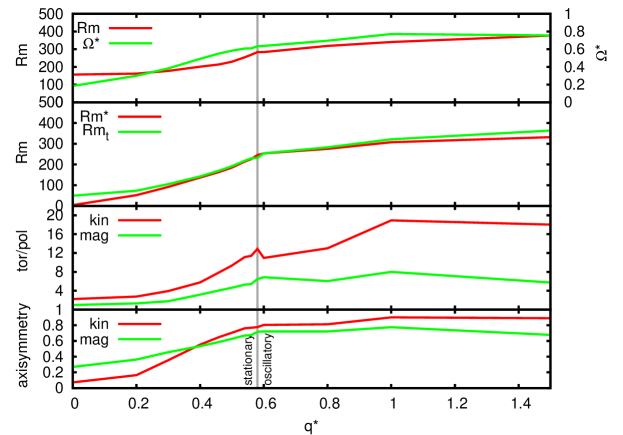
Figure 2: First panel: magnetic Reynolds number and the relative amount of toroidal field induced by the axisymmetric $\Omega$-effect as a function of the heat flux anomaly amplitude $q^{\star}$. Second panel: magnetic Reynolds number based only on the axisymmetric and equatorially antisymmetric zonal flows $Rm^{\star}$ and the strength of thermal wind $Rm_{t}$ according to eq. 11. Third panel: ratio of toroidal to poloidal kinetic and magnetic energy. Bottom panel: relative axisymmetry in the kinetic and magnetic energy. The gray vertical line at $q^{\star}\approx 0.6$ denotes the onset of the oscillations.

3 Results

Figure 1 illustrates the effect of the latitudinal heat flux variation on the convection and induction mechanism. For a homogeneous heat flux the temperature and the weak zonal flow are symmetric with respect to the equator (fig. 1 a), whereas the magnetic field is antisymmetric (fig. 1 b and c). If a sufficiently strong heat flux anomaly is applied, here $q^{\star}=1.0$, the temperature shows a strong gradient in latitudinal direction that penetrates deep into the shell (fig. 1 d). Northward directed flows tend to equilibrate the latitudinal temperature anomaly and are diverted by the Coriolis force into the azimuthal direction. This effect is known as thermal wind and relates latitudinal gradients in the axisymmetric temperature $\overline{T}$ with zonal flow $\overline{u}_{\varphi}$ gradients parallel to the axis of rotation

$$\frac{\partial\overline{u}_{\varphi}}{\partial z}=Ra_{q}^{\star}Pm\frac{1}{2r_{o}}\frac{\partial\overline{T}}{\partial\vartheta}\ .$$ (10)

Toroidal field is mainly produced by an $\Omega$-effect associated with the shear between the retrograde zonal flow in the northern hemisphere and the prograde zonal flow in the southern hemisphere (fig. 1 e). Convective columns are largely missing and the small-scale convective flow is dominated by plume-like up- and downwellings in the southern hemisphere. Since these are the major source for helical motions, the $\alpha$-effect and thus poloidal field production is concentrated in the southern hemisphere (fig. 1 e and f).

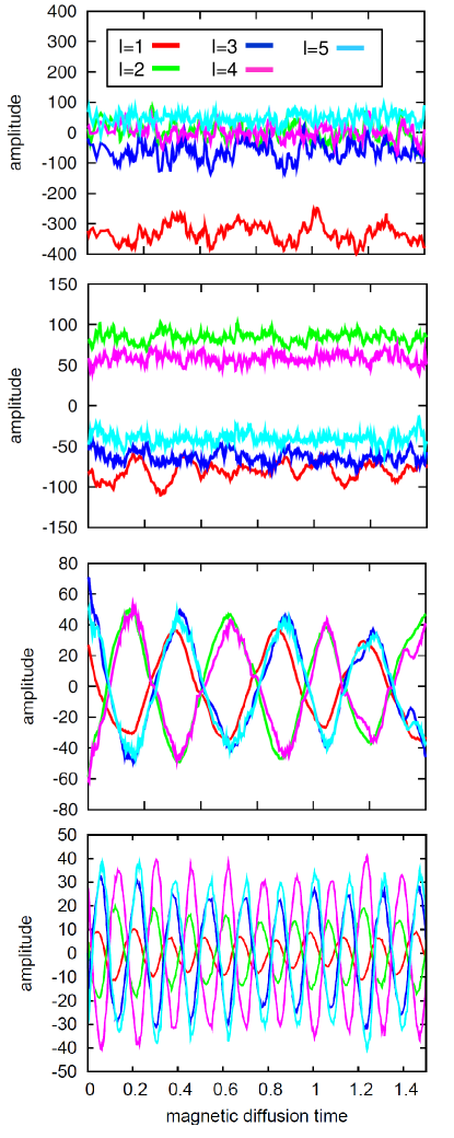
Figure 3: Time evolution of the Gauss coefficients for $q^{\star}=0,0.5,0.6,1$ (from top to bottom). Colour coded are the first five axisymmetric coefficients of degree $l=1,2,3,4,5$ in red, green, dark blue, pink and light blue.

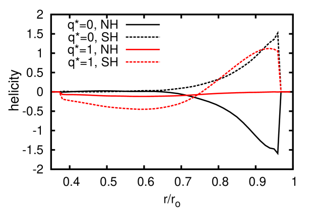
Figure 4: Radial profiles of the horizontally averaged kinetic helicity for the southern (SH) and northern hemisphere (NH).

Fig. 2 demonstrates how the flow and the magnetic field becomes predominantly axisymmetric and toroidal when the amplitude $q^{\star}$ increases. Since the axisymmetric toroidal flow contribution is identical to the axisymmetric azimuthal (or zonal) flow this illustrates the dominant role of thermal winds at larger $q^{\star}$ values. In the scaling used here, the magnetic Reynolds number $Rm=uD/\lambda$ corresponds to the velocity. In fig. 2, second panel we test the influence of the thermal wind by comparing the flow amplitude based on the equatorially antisymmetric and axisymmetric flow $Rm^{\star}$ with the amplitude of the thermal wind $Rm_{t}$ controlled by

$$Rm_{t}=Ra_{q}^{\star}Pm\frac{l_{z}}{2r_{o}}\left\langle\frac{\partial\overline{T}}{\partial\vartheta}\right\rangle_{\mathrm{rms}}\ .$$ (11)

Here, $l_{z}$ is the typical length scale for zonal flow variations in the direction of the rotation axis and is taken to be half the height of the spherical shell at mid-depth ($l_{z}\approx 1.18$). The good agreement shows that the equatorially antisymmetric zonal flow originates from thermal wind alone. In the regime $q^{\star}\geq 0.6$ both the thermal wind magnetic Reynolds number estimate $Rm_{t}$ and $Rm^{\star}$ approaches the true magnetic Reynolds number $Rm$ as is shown in fig. 2. This demonstrates the thermal wind origin of the fierce zonal flows.

We further quantify the relative importance of the $\Omega$-effect in toroidal field production by :

$$\Omega^{\star}=\frac{\langle\bf{B}\cdot\bf{\nabla}\overline{u}_{\varphi}\rangle^{\mathrm{tor}}_{\mathrm{rms}}}{\langle\bf{B}\cdot\bf{\nabla}\bf{u}\rangle_{\mathrm{rms}}^{\mathrm{tor}}}\ .$$ (12)

Fig. 2 illustrates that $\Omega^{\star}$ indeed increases beyond $0.5$ once $q^{\star}\geq 0.6$. For a homogeneous heat flux ($q^{\star}=0$) the $\Omega$-effect is negligible. The latitudinal heat flux variation thus clearly changes the dynamo mechanism from an $\alpha^{2}$ to an $\alpha^{2}\Omega$ or $\alpha\Omega$ type. The effective $\Omega$-effect has the consequence that the magnetic field is dominated by the axisymmetric toroidal magnetic field as is shown in the lower panels of fig. 2. Strong Lorentz forces associated to this field component nearly completely suppress the convective columns at larger $q^{\star}$ values Dietrich and Wicht (2013); Stanley et al. (2008).

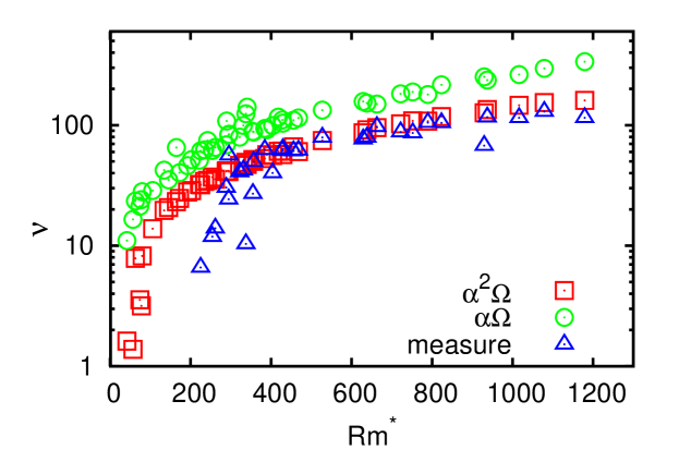
Figure 5: Frequencies measured from the evolution of the Gauss coefficients (blue triangles), the frequencies calculated by the $\alpha\Omega$ (eq. 8, green circles) and the $\alpha^{2}\Omega$ (eq. 9, red squares) dispersion relation as function of the zonal flow amplitude given by $Rm^{\star}$.

The onset of the dynamo wave is roughly found where the $\Omega$-effect starts to play a dominant role at $q^{\star}\approx 0.6$. Fig. 3 shows the time evolution of the leading axisymmetric Gauss coefficients describing the magnetic field at the top of the dynamo region. In the reference case ($q^{\star}=0$) the dipole contribution clearly dominates. When the perturbation is increased to $q^{\star}=0.5$, the even and odd modes reach similar amplitudes but have opposite sign. This reflects a hemispherical magnetic field concentrated in the southern hemisphere (2nd panel). The time dependence is still ruled by the turbulent convective flow dynamics as in the reference case. A further increase of the heat flux variation to $q^{\star}=0.6$ finally promotes the onset of the dynamo wave. Even and odd modes oscillate periodically in antiphase with nearly similar amplitudes. If $q^{\star}$ is further increased, both the thermal wind shearing (see $Rm^{\star}$ in fig. 2) and the frequency of the oscillation grow. This is the expected behaviour of a mean-field Parker wave Schrinner et al. (2007), as shown in the dispersion relation (eqs. 8 and 9). In a numerical test, we switched off the Lorentz force in our simulation. The oscillation persisted as a purely kinematic effect which is a key feature of Parker waves.

To more qualitatively test whether the os¡cillation obeys the Parker wave dispersion relation (eq. 8 and 9) we have to estimate the wave numbers, the $\Omega$-effect or latitudinal shear, and the $\alpha$-effect via the helicity Tobias and Weiss (2007). For the large-scale wave behaviour we simply approximate the wave numbers $k_{2},k_{3}$ with $2\pi$-th of the inverse characteristic length scales $l_{i}$. We choose $l_{2}\approx\pi$ as half the circumference along latitude at mid-depth, and $l_{3}=1$ as the shell thickness. The latitudinal shear is estimated with $\partial\overline{u}/\partial x_{2}\approx Rm^{\star}/\pi$. The $\alpha$-term is approximated via $\alpha=-H\,\tau/3$ where $\tau$ is the correlation time and $H$ is the kinetic helicity Krause and Rädler (1980).

We further assume that $\tau$ is the mean flow overturn time $\ell/Rm^{\prime}$ where $Rm^{\prime}$ quantifies the mean amplitude of the non-axisymmetric flow and $\ell$ is its typical length scale estimated from the spectra of the poloidal flow.

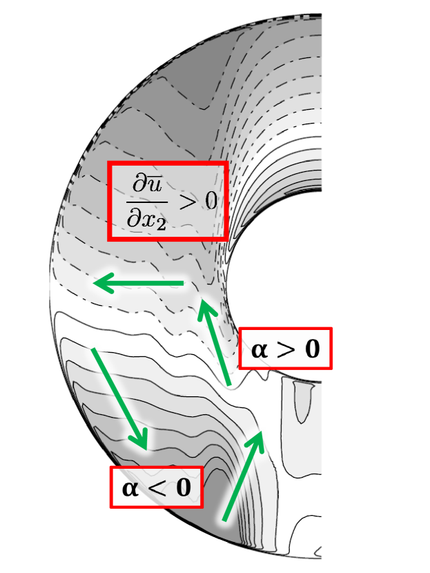
Figure 6: Angular velocity in gray scale, signs of $\alpha$ and $\Omega$-effect (red) and theoretical propagation direction of $\alpha\Omega$ waves (green arrows).

Estimating the helicity is more involved. Fig. 4 shows radial profiles of the rms helicity in the northern and southern hemispheres for the homogeneous reference case and the hemispherical $q^{\star}=1.0$ case. The helicity $H=\bf{u}^{\prime}\cdot\bf{\nabla}\times\bf{u}^{\prime}$ is averaged either over the southern (dashed lines) or the northern hemisphere (solid). Note that only the non-axisymmetric flow components are used here. In the reference case ($q^{\star}=0$, black) the helicity is negative in the northern, positive in the southern hemisphere and antisymmetric with respect to the equator. Such a configuration is essential for creating dipole dominated magnetic fields. In the hemispherical solution, the northern hemisphere is devoid of helicity (red solid), whereas in the southern hemisphere (red dashed) the sign changes from negative in the inner part to positive in the outer part of the dynamo shell. Since the dynamo wave is concentrated to the southern hemisphere we use only the rms helicity in this hemisphere to estimate $\alpha$.

In fig. 5 we compare the predicted frequencies $\nu_{\alpha\Omega}$ and $\nu_{\alpha^{2}\Omega}$ according to eqs. 8 and 9 with the measured frequency for $51$ simulations at different parameters. They cover Ekman numbers from $E=3\times 10^{-4}$ to $E=3\times 10^{-5}$, magnetic Prandtl numbers from $Pm=1$ to $Pm=5$, and a broad range of Rayleigh numbers and $q^{\star}$ values. The zonal flow magnetic Reynolds number $Rm^{\star}$ used for the $x$-axis of fig. 5 mainly depends on $q^{\star}$. Since the dynamo waves only set in at larger $q^{\star}$ values there are no measured frequencies at low $Rm^{\star}$. Also we expect an improved fit to the prediction at larger $Rm^{\star}$ values where axisymmetric toroidal field and flow clearly dominate. Considering the various simplifications and approximations involved the agreement between measured and predicted frequencies seems convincing enough to establish the Parker wave nature of the oscillations. The $\alpha^{2}\Omega$ frequencies $\nu_{\alpha^{2}\Omega}$ are always smaller than the $\nu_{\alpha\Omega}$, since the second $\alpha$-effect reduces the frequency. However, the data scatter seem too large to distinguish whether the mechanism is of the $\alpha\Omega$- or the $\alpha^{2}\Omega$-type.

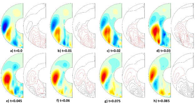
Figure 7: Temporal evolution of the axisymmetric toroidal field (left) and poloidal field lines (right) during half a wave cycle. Note, that the time difference between two shown snapshots changes non-equidistantly.

The propagation behaviour is another key spotting feature for Parker waves Yoshimura (1976). In general, a Parker wave travels along lines of constant shear and its direction depends on the sign of the product of the $\alpha$- and $\Omega$-effect Tobias and Weiss (2007). Since the northern zonal flow cell is progressing westward (slower than average) and the southern eastward (faster than average) the $\Omega$-effect $\partial\overline{u}/\partial x_{2}$ is positive everywhere (see fig. 6). The helicity changes its sign at some depth in the shell for strongly hemispherical solutions (see fig. 4). Fig. 6 illustrates the resulting propagation path expected for a Parker wave in the hemispherical cases. This is consistent with the observed propagation of the dynamo wave shown in fig. 7. Suppose the wave cycle starts at lower southern latitudes close to the outer boundary (small red patch, fig. 7, first plot) with a poleward and inward migration of the field. Due to the strong $\alpha$-effect the field is amplified and propagates further northwards, replacing the inverse polarity. At the equator the wave migrates along lines of constant shear (radially outward here).

4 Discussion

We demonstrated that the oscillating solution found in strongly hemispherical dynamo solutions promoted by a north/south heat flux asymmetry through the outer boundary are likely Parker dynamo waves. The heat flux pattern leaves the northern hemisphere hotter than the southern and the associated temperature gradient drives fierce zonal thermal winds. These in turn lead to a strong $\Omega$-effect, a prerequisite for Parker waves.

In the Martian context this is bad news because the relatively fast oscillations on the order of a few thousand years are not compatible with the high crustal magnetization amplitude Dietrich and Wicht (2013). Since crustal magnetization is acquired over several million years the effective magnetization as observed from a space craft would be very weak.

Lateral heat flux variations with $q^{\star}\approx 1$ seem generally possible for terrestrial planets, at least as long as the mantle is actively convecting. The large-scale cosine-like variation explored here, however, is geared to explain the Martian hemisphericity. For Earth, the heat flux pattern is dominated by a spherical harmonic of degree and order two. This was likely different in the past, but a degree one pattern nevertheless seems more likely for Mars while higher harmonics are expected for Earth Roberts and Zhong (2006). Another property essential for promoting strong thermal winds is the dynamo heating mode. The effect of an outer boundary heat flux variation is much larger for a dynamo without an inner core that is exclusively driven by secular cooling Hori et al. (2012). Whether a combination of a more complex heat flux pattern and secular cooling would also lead to strong thermal winds and possibly Parker waves has not been explored in any detail so far. This may have been the case for the geodynamo before the onset of inner core growth which may have happened only one Gyr ago.

Recent simulations geared to model the dynamo in the gas giants also show oscillatory behaviour reminiscent of Parker waves Gastine et al. (2012). Here the stress free outer boundaries allow much stronger zonal winds to develop than in typical simulations for terrestrial dynamos. This can also lead to a strong $\Omega$-effect and associated Parker wave behaviour. Parker waves are thus not only interesting to explain the solar cycle but also have to be considered in the planetary context.

References

- Acuña et al. [1999] M. H. Acuña, J. E. P. Connerney, N. F. Ness, R. P. Lin, D. Mitchell, C. W. Carlson, J. McFadden, K. A. Anderson, H. Reme, C. Mazelle, D. Vignes, P. Wasilewski, and P. Cloutier. Global Distribution of Crustal Magnetization Discovered by the Mars Global Surveyor MAG/ER Experiment. Science, 284:790–793, April 1999. 10.1126/science.284.5415.790.
- Busse and Simitev [2006] F. H. Busse and R. D. Simitev. Parameter dependences of convection-driven dynamos in rotating spherical fluid shells. Geophys. Astrophys. Fluid Dyn., 100:341–361, October 2006. 10.1080/03091920600784873.
- Dietrich and Wicht [2013] W. Dietrich and J. Wicht. A hemispherical dynamo model: Implications for the martian crustal magnetization. Phys. Earth Planet. Inter., 217:10 – 21, 2013. ISSN 0031-9201. 10.1016/j.pepi.2013.01.001.
- Gastine et al. [2012] T. Gastine, L. Duarte, and J. Wicht. Dipolar versus multipolar dynamos: the influence of the background density stratification. Astron. Astrophys., 546:A19, October 2012. 10.1051/0004-6361/201219799.
- Grote and Busse [2000] E. Grote and F. H. Busse. Hemispherical dynamos generated by convection in rotating spherical shells. Phys. Rev. E, 62:4457–4460, September 2000. 10.1103/PhysRevE.62.4457.
- Hori et al. [2012] K. Hori, J. Wicht, and U. R. Christensen. The influence of thermo-compositional boundary conditions on convection and dynamos in a rotating spherical shell. Phys. Earth Planet. Inter., 196:32–48, April 2012. 10.1016/j.pepi.2012.02.002.
- Krause and Rädler [1980] F. Krause and K.-H. Rädler. Mean-field magnetohydrodynamics and dynamo theory. 1980.
- Olson et al. [1999] P. Olson, U. Christensen, and G. A. Glatzmaier. Numerical modeling of the geodynamo: Mechanisms of field generation and equilibration. J. Geophys. Res., 1041:10383–10404, May 1999. 10.1029/1999JB900013.
- Parker [1955] E. N. Parker. Hydromagnetic Dynamo Models. Astrophys. J., 122:293, September 1955. 10.1086/146087.
- Roberts and Zhong [2006] J. H. Roberts and S. Zhong. Degree-1 convection in the Martian mantle and the origin of the hemispheric dichotomy. J. Geophys. Res., 111:6013–6035, June 2006. 10.1029/2005JE002668.
- Rüdiger and Hollerbach [2004] G. Rüdiger and R. Hollerbach. The magnetic universe: geophysical and astrophysical dynamo theory. August 2004.
- Schrinner et al. [2007] M. Schrinner, K.-H. Rädler, D. Schmitt, M. Rheinhardt, and U. R. Christensen. Mean-field concept and direct numerical simulations of rotating magnetoconvection and the geodynamo. Geophys. Astrophys. Fluid Dyn., 101:81–116, April 2007. 10.1080/03091920701345707.
- Schrinner et al. [2011] M. Schrinner, L. Petitdemange, and E. Dormy. Oscillatory dynamos and their induction mechanisms. Astron. Astrophys, 530:A140, June 2011. 10.1051/0004-6361/201016372.
- Stanley et al. [2008] S. Stanley, L. Elkins-Tanton, M. T. Zuber, and E. M. Parmentier. Mars´Paleomagnetic Field as the Result of a Single-Hemisphere Dynamo. Science, 321:1822–, September 2008. 10.1126/science.1161119.
- Tobias and Weiss [2007] S. Tobias and N. Weiss. Linear -dynamos for the solar cycle. In Dormy, E. and Soward, A. M., editor, Mathematical Aspects of Natural Dynamos, The Fluid Mechanics of Astrophysics and Geophysics, pages 281–312. Grenoble Sciences, 2007.
- Wicht [2002] J. Wicht. Inner-core conductivity in numerical dynamo simulations. Phys. Earth Planet. Inter., 132:281–302, October 2002.
- Yoshimura [1976] H. Yoshimura. Phase relation between the poloidal and toroidal solar-cycle general magnetic fields and location of the origin of the surface magnetic fields. Solar Phys., 50:3–23, October 1976. 10.1007/BF00206186.