Resonant metamaterial absorbers for infrared spectral filtering: quasimodal analysis, design, fabrication and characterization

Abstract

We present a modal analysis of metal-insulator-metal (MIM) based metamaterials in the far infrared region. These structures can be used as resonant reflection bandcut spectral filters that are independent of the polarization and direction of incidence because of the excitation of quasimodes (modes associated with a complex frequency) leading to quasi-total absorption. We fabricated large area samples made of chromium nanorod gratings on top of Si/Cr layers deposited on silicon substrate and measurements by Fourier Transform spectrophotometry show good agreement with finite element simulations. A quasimodal expansion method is developed to obtain a reduced order model that fits very well full wave simulations and that highlights excitation conditions of the modes.

I Introduction

Structuration of metallic surfaces with typical size smaller than the wavelength can lead to spectacular resonant effects. More than one century ago, anomalies in reflection of metallic gratings have been discovered by Wood Wood (1902), and substantial pioneering work Hutley and Maystre (1976); Hessel and Oliner (1965) have highlighted the role of surface plasmons polaritons in the anomalous reflection in mono and bi-periodic gratings. These resonances can be used to fashion various reflection and transmission spectra. In particular, total absorption phenomena in different metamaterial type Teperik et al. (2008); Landy et al. (2008); Bonod et al. (2008); Tao et al. (2008); Hao et al. (2010) from the micro wave to optical regime, have recently attracted a lot of interest because of their potential application in sensing Liu et al. (2010), tunable frequency selective microbolometers Maier and Brückl (2009); Maier and Brueckl (2010) or solar cells Teperik et al. (2008). One family of metamaterial have been extensively studied which is based on Metal-Insulator-Metal (MIM)configuration Hao et al. (2010); Aydin et al. (2011); Bouchon et al. (2012); Hao et al. (2011), because they can lead to polarization and angle independent resonant perfect absorption. This is the kind of structures we study both numerically and experimentally in this paper with the aim of using them as bandcut reflection filters in the infrared that can be tuned by adjusting the periodicity of the grating.
Besides the calculation of diffraction efficiencies and absorption spectra, our approach to study the resonant phenomena in such metamaterials is to compute the eigenmodes and eigenfrequencies of such open electromagnetic systems. The study of poles and zeros of the scattering operator Popov et al. (1986); Nevière et al. (1995) and of their associated leaky modes leads to significant insights into the properties of metamaterials Tikhodeev et al. (2002); Fehrembach and Sentenac (2003); Lalanne et al. (2006); Grigoriev et al. (2013) and eases the conception diverse optical devices Fehrembach and Sentenac (2005); Sentenac and Fehrembach (2005); Ding and Magnusson (2004a, b, c) because it provides a simple picture of the resonant processes at stake. From the resolution of a spectral problem, one obtains complex eigenfrequencies. The real part is the resonant frequency and the imaginary part the bandwidth. Resonant scattering is expected when shining light with frequency around the resonant frequency. We report here a numerical spectral analysis of MIM arrays, that allows us to optimize parameters for infrared reflection bandcut filters. The spectral position od the reflection dip can be adjusted by varying the periodicity of the grating. Large area samples with different periods have been fabricated and characterized by FTIR spectroscopy, and measured normal incidence reflection spectra agree well with the numerical predictions of both calculated reflection spectra and complex eigenvalues. Moreover, the high angular tolerance of the filters is demonstrated experimentally and numerically.
The eigenvectors and eigenvalues are intrinsic properties of the studied system that depends onto the opto-geometrical parameters but are in essence independent of the incident parameters. Our main contribution is to provide a systematic method to characterize the excitation of a given mode. By expanding the scattered field onto the eigenmode basis, we can compute the coupling coefficient that characterizes the strength of the interaction of incident light with a mode. This method is illustrated in the case of a MIM array, showing the resonant nature of the reflection dip and providing a reduced-order model with two degenerate leaky modes that fits very well full wave finite elements calculation.

II Setup of the problem and theoretical background

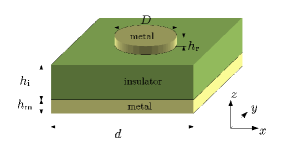
(a)

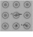
(b)

Figure 1: Geometry of the studied structures. (a): schematic representation and notations. (b): SEM image (top view) of a fabricated grating.

II.1 Diffraction problem

The geometry of the structures studied in this paper is represented in Fig. 1(a) and consist of three layers. The top layer is made of a square array with period $d$ along both $Ox$ and $Oy$ of cylindrical chromium nanorods with diameter $D$ and thickness $h_{\rm r}$. The bottom layer is a continuous chromium film of thickness $h_{\rm m}$. These two metallic layers are separated by an amorphous silicon film of thickness denoted $h_{\rm i}$. The incident medium (superstrate) is air with permittivity $\varepsilon^{+}=1$ and the structure are deposited on a silicon substrate with permittivity $\varepsilon^{-}$. The permittivity of chromium is described by a Drude-Lorentz model Lovrinčić and Pucci (2009) and the refractive index of bulk and amorphous silicon are taken from tabulated data Palik (1991). All materials are assumed to be non magnetic ($\mu_{r}=1$).
We consider here the time-harmonic regime with $\mathrm{e}^{-i\omega t}$ dependance. The structure is illuminated by a plane wave $\bm{E}^{\mathrm{inc}}=\bm{A}^{\mathrm{0}}\;\textrm{exp}(i\,\bm{k}^{+}\cdot\bm{r})$ with

$$\bm{k}^{+}=\left|\begin{array}[]{l}\alpha\\ \beta\\ \gamma\end{array}\right.=k^{+}\left|\begin{array}[]{l}-\sin\theta_{0}\,\cos\varphi_{0}\\ -\sin\theta_{0}\,\sin\varphi_{0}\\ -\cos\theta_{0}\end{array}\right.$$

and

$$\bm{A}_{0}^{e}=\left|\begin{array}[]{l}E^{0}_{x}\\ E^{0}_{y}\\ E^{0}_{z}\end{array}\right.=A^{e}\left|\begin{array}[]{l}\cos\psi_{0}\,\cos\theta_{0}\,\cos\varphi_{0}-\sin\psi_{0}\,\sin\varphi_{0}\\ \cos\psi_{0}\,\cos\theta_{0}\,\sin\varphi_{0}+\sin\psi_{0}\,\cos\varphi_{0}\\ -\cos\psi_{0}\,\sin\theta_{0}\end{array}\right.$$

where $\varphi_{0}\in[0,2\pi]$, $\theta_{0}\in[0,\frac{\pi}{2}]$, $\psi_{0}\in[0,\pi]$, $k_{0}=\omega/c$ and $k^{+}=k_{0}\sqrt{\varepsilon^{+}}$.
The problem we are dealing with is to find non trivial solutions of Maxwell’s equation, i. e. to find the unique electromagnetic field $(\bm{E},\bm{H})$ such that

$$\mathcal{L}_{\bm{\varepsilon},\bm{\mu}}(\bm{E}):=-\bm{\mathrm{\nabla\times}}\left(\bm{\mu}^{-1}\,\bm{\mathrm{\nabla\times}}\bm{E}\right)+k_{0}^{2}\,\bm{\varepsilon}\,\bm{E}={\bm{0}},$$ (1)

where the diffracted field $\bm{E}^{d}=\bm{E}-\bm{E}^{\rm inc}$ satisfies an outgoing wave condition (OWC) and where $\bm{E}$ is quasiperiodic along $x$ and $y$

$$\bm{E}(x+d_{x},y+d_{y},z)=\bm{E}(x,y,z)\mathrm{e}^{i(\alpha d_{x}+\beta d_{y})}.$$

Under this form, the problem is not adapted to a resolution by a numerical method because of infinite issues: the sources of the plane wave are infinitely far above the structure, the geometric domain is unbounded and the scattering structure is itself infinitely periodic. To circumvent these issues, we compute only the diffracted field solution of an equivalent radiation problem with sources inside the scatterers, we use PMLs to truncate the unbounded domain at a finite distance, and we use quasiperiodicity conditions to model a single period of the grating.
Denoting $\bm{\varepsilon_{1}}$ and $\bm{\mu_{1}}$ the tensor fields describing the multilayer problem, the function $\bm{E}_{1}$ is defined as the unique solution of $\mathcal{L}_{\bm{\varepsilon_{1}},\bm{\mu_{1}}}(\bm{E}_{1})=0$, such that $\bm{E}_{1}^{d}:=\bm{E}_{1}-\bm{E}_{0}$ satisfies an OWC. The expression of this function can be calculated with a matrix transfer formalism extensively used in thin film optics (See for example Ref. Macleod (2001)). The unknown function $\bm{E}_{2}^{d}$ is thus given by $\bm{E}_{2}^{d}=\bm{E}-\bm{E}_{1}=\bm{E}^{d}-\bm{E}_{1}^{d}$. The scattering problem (1) can be rewritten as:

$$\mathcal{L}_{\bm{\varepsilon},\bm{\mu}}(\bm{E}_{2}^{d})=-\mathcal{L}_{\bm{\varepsilon_{1}},\bm{\mu_{1}}}(\bm{E}_{1}):=\bm{\mathcal{S}}_{1}.$$ (2)

The term on the right hand side can be seen as a source term $\bm{\mathcal{S}}_{1}$ with support in the diffractive objects $\Omega_{g^{\prime}}$ and is known in closed form Demésy et al. (2009).
The radiation problem defined by Eq. (2) is then solved by the FEM Demésy et al. (2007, 2009, 2009), using PMLs to truncate the infinite regions and by setting convenient boundary conditions on the outermost limits of the domain. We apply Bloch quasiperiodicity conditions with coefficient $\alpha$ (resp. $\beta$) on the two parallel boundaries orthogonal to $x$ (resp. $y$), and homogeneous Dirichlet boundary conditions on the outward boundary of the PMLs. The computational cell is meshed using $2\textsuperscript{nd}$ order edge elements. The final algebraic system is solved using a direct solver (PARDISO Schenk and Gärtner (2004)).

II.2 Spectral problem

The diffractive properties of open waveguides such as those studied here are governed by their eigenmodes and eigenfrequencies. The eigenproblem we are dealing with consists in finding the solutions of source free Maxwell’s equations, i.e. finding eigenvalues ${\Lambda_{n}}=({\omega}_{n}/c)^{2}$ and non zero eigenvectors $\bm{V}_{n}$ such that:

$$\mathcal{M}_{\bm{\mu}}(\bm{V}_{n}):=\bm{\mathrm{\nabla\times}}\left(\bm{\mu}^{-1}\,\bm{\mathrm{\nabla\times}}\bm{V}_{n}\right)=\Lambda_{n}\,\bm{\varepsilon}\,\bm{V}_{n}.$$ (3)

Note that we search for Bloch-Floquet eigenmodes so Maxwell’s operator $\mathcal{M}_{\bm{\mu}}$ is parametrized by the real quasiperiodicity coefficients $\alpha$ and $\beta$. Because we are dealing with an open structure, the eigenvalues $\Lambda_{n}$ are complex even for Hermitian materials. The spectrum of the associated Maxwell’s operator is constituted of a continuous part corresponding to radiation modes and a discrete set of complex eigenvalues associated with the so-called quasimodes (also known as leaky modes or resonant states). PMLs have proven to be a very convenient tool to compute leaky modes in various configurations Ould Agha et al. (2008); Popovic (2003); Hein et al. (2004); Eliseev et al. (2005) because they mimic efficiently the infinite space provided a suitable choice of their parameters. Indeed, if we choose a constant stretching parameter $\zeta$ for the PMLs, it is sufficient to take $\mathfrak{Re}(\zeta)>0$ and $\mathfrak{Im}(\zeta)>0$ to rotate the continuous spectrum in the lower half complex plane $\mathfrak{Re}(\omega)<0$, which reveals outgoing quasimodes (satisfying outgoing wave conditions) Vial et al. (2014). It is well known that the associated eigenvalues are poles of the scattering matrix. In addition, the zeros $\Lambda^{z}_{n}$ of the scattering matrix are associated with incoming quasimodes (satisfying incoming wave conditions), that we can compute by setting $\mathfrak{Re}(\zeta)>0$ and $\mathfrak{Im}(\zeta)<0$ leading to a displacement of the continuous spectrum in the upper half complex plane $\mathfrak{Re}(\omega)>0$. A real zero $\Lambda^{z}$ indicates total absorption of incident light.
Note that the incident angles $\theta_{0}$ et $\varphi_{0}$ appear in a subtle way through the quasiperiodicity coefficients $\alpha$ et $\beta$, but the polarization angle $\psi_{0}$ does not come into play in the spectral problem. It is thus necessary to thoroughly study eigenmodes in order to find the polarization state that can excite the modes at stake.

The eigenvalue problem defined by Eq. (3) is solved with the FEM as described in section II.1. We have supposed here that the material are non dispersive, which makes the problem in Eq. (3) linear. To take into account dispersion, the eigenvalue problem is solved iteratively with updated values of permittivity. This procedure converges rapidly due to the slow variations of the permittivity of the considered materials in the far infrared range.

II.3 Quasimodal expansion method

We first define the classical inner product of two functions $\bm{F}$ and $\bm{G}$ of $L^{2}(\Omega)$, $\Omega\subset\mathbb{R}^{3}$:

$$\left\langle\bm{F}\,\middle|\,\bm{G}\right\rangle:=\int_{\Omega}\bm{F}(\bm{r})\cdotp\vbox{ \hrule height=0.3pt\kern 2.15277pt\hbox{ \kern-3.99994pt$\bm{G}(\bm{r})$\kern 0.0pt} }\;\mathrm{d}\bm{r}.$$ (4)

Unlike self-adjoint problems, $\left\langle\bm{\varepsilon}\bm{V}_{n}\,\middle|\,\bm{V}_{m}\right\rangle\neq\delta_{nm}$, in other words the eigenmodes $\bm{V}_{n}$ are not orthogonal with respect to this standard definition. This is the reason why we consider an adjoint spectral problem with eigenvalues $\vbox{ \hrule height=0.3pt\kern 2.15277pt\hbox{ \kern-3.99994pt$\Lambda_{n}$\kern 0.0pt} }=(\vbox{ \hrule height=0.3pt\kern 2.15277pt\hbox{ \kern-3.99994pt$\omega_{n}$\kern 0.0pt} }/c)^{2}$ and eigenvectors $\bm{W}_{n}$. The adjoint operator $\mathcal{M}^{\dagger}_{\bm{\mu}}$ is defined by

$$\left\langle\vphantom{\mathcal{M}^{\dagger}_{\bm{\mu}}(\bm{W})}\mathcal{M}_{\bm{\mu}}(\bm{V})\,\middle|\,\bm{W}\right\rangle=\left\langle\bm{V}\,\middle|\,\mathcal{M}^{\dagger}_{\bm{\mu}}(\bm{W})\right\rangle$$ (5)

with complex conjugate coefficients for the boundary conditions in comparison with the direct spectral problem , and is such that $\mathcal{M}^{\dagger}_{\bm{\mu}}=\mathcal{M}_{\bm{\mu}^{\star}}$, where $A^{\star}={\vbox{ \hrule height=0.3pt\kern 2.15277pt\hbox{ \kern-3.99994pt$A$\kern 0.0pt} }}^{\mathrm{T}}$ is the conjugate transpose of matrix $A$. The associated adjoint problem that we shall solve is:

$$\mathcal{M}^{\dagger}_{\bm{\mu}}(\bm{W}_{n})=\bm{\mathrm{\nabla\times}}\left({\bm{\mu}^{\star}}^{-1}\,\bm{\mathrm{\nabla\times}}\bm{W}_{n}\right)=\vbox{ \hrule height=0.3pt\kern 2.15277pt\hbox{ \kern-3.99994pt$\Lambda_{n}$\kern 0.0pt} }\,{\bm{\varepsilon^{\star}}}\,\bm{W}_{n}.$$ (6)

We know from spectral theory that the eigenvectors $\bm{V}_{n}$ are bi-orthogonal to their adjoint counterparts $\bm{W}_{n}$ Hanson and Yakovlev (2002):

$$\left\langle\bm{\varepsilon}\bm{V}_{n}\,\middle|\,\bm{W}_{m}\right\rangle:=\int_{\Omega}\bm{\varepsilon}(\bm{r})\,\bm{V}_{n}(\bm{r})\cdotp\vbox{ \hrule height=0.3pt\kern 2.15277pt\hbox{ \kern-3.99994pt$\bm{W}_{m}(\bm{r})$\kern 0.0pt} }\;\mathrm{d}\bm{r}=K_{n}\delta_{nm},$$ (7)

where the normalization coefficient $K_{n}=\left\langle\bm{\varepsilon}\bm{V}_{n}\,\middle|\,\bm{W}_{n}\right\rangle$. Relation (7) provides a complete bi-orthogonal set to expand every field solution of Eq. (2) propagating in the open waveguide as:

$$\displaystyle\bm{E}_{2}^{d}(\bm{r},\omega,\psi) = \sum_{n=1}^{+\infty}P_{n}(\omega,\psi)\,\bm{V}_{n}(\bm{r})$$ (8)

$$+\int_{\Gamma_{c}}P_{\nu}(\omega,\psi)\,\bm{V}_{\nu}(\bm{r})\;\mathrm{d}\nu,$$

where $\Gamma_{c}$ is the continuous spectrum (a curve, with possibly a denombrable set of branches in the complex plane). The coefficients $P_{k}(\omega,\psi)$, $k=\{n,\nu\}$, are given by:

$$P_{k}(\omega,\psi)=\frac{1}{K_{k}}\left\langle\bm{\varepsilon}\bm{E}_{2}^{d}\,\middle|\,\bm{W}_{k}\right\rangle=\frac{J_{k}(\omega,\psi)}{{\omega}^{2}-\omega_{k}^{2}},$$ (9)

with

$$J_{k}(\omega,\psi) = \frac{c^{2}}{K_{k}}\left\langle\bm{\mathcal{S}}_{1}\,\middle|\,\bm{W}_{k}\right\rangle$$ (10)

$$= \frac{c^{2}}{K_{k}}\int_{\Omega_{g^{\prime}}}\bm{\mathcal{S}}_{1}(\bm{r},\omega,\psi)\,\vbox{ \hrule height=0.3pt\kern 2.15277pt\hbox{ \kern-3.99994pt$\bm{W}_{k}(\bm{r})$\kern 0.0pt} }\;\mathrm{d}\bm{r},$$

where the integration is only performed on the inhomogeneities $\Omega_{g^{\prime}}$ since the source term $\bm{\mathcal{S}}_{1}$ is zero elsewhere. Note that the last integral has to be taken in the distributional meaning which leads to a surface term on $\partial\Omega_{g^{\prime}}$ because of the spatial derivatives in $\bm{\mathcal{S}}_{1}$.
We are thus able to know how a given mode is excited when changing the incident field. This modal expansion can be approximated by a discrete sum since the spectrum of the final operator we solve for involves only discrete eigenfrequencies, and in practice only a finite number $M$ of modes is retained in the expansion, so that we can write:

$$\bm{E}_{2}^{d}(\bm{r},\omega,\psi)\simeq\sum_{m=1}^{M}P_{m}(\omega,\psi)\,\bm{V}_{m}(\bm{r}).$$ (11)

This leads to a reduced modal representation of the field which is well adapted when studying the resonant properties of the open structure, as illustrated in the sequel.

III Modal analysis of MIM arrays

The parameters employed are $h_{\rm r}=$100\text{\,}\mathrm{n}\mathrm{m}$$, $h_{\rm i}=$530\text{\,}\mathrm{n}\mathrm{m}$$, $h_{\rm m}=$200\text{\,}\mathrm{n}\mathrm{m}$$, and we fix the ratio between the rod diameter and the period $f=D/d=0.5$. We study the influence of the period $d$ on the reflection spectrum of the metamaterial.

III.1 Fabrication and characterization of the samples

Samples with parameters described above and varying period of $4.0$, $4.4$, $4.8$, $5.2$ and $5.6\text{\,}\mathrm{\SIUnitSymbolMicro m}$ have been fabricated (a SEM image showing a top view of the filter with $d=$4\text{\,}\mathrm{\SIUnitSymbolMicro m}$$ is given in Fig 1(b)). The different layers have been deposited by magnetron sputtering on a standard silicon wafer of diameter $100\text{\,}\mathrm{mm}$ and thickness $525\text{\,}\mathrm{\SIUnitSymbolMicro m}$. Large area samples ($$1\text{\,}\mathrm{cm}$\times$1\text{\,}\mathrm{cm}$$) were patterned with a standard photolithography process with a positive resist deposition followed by a chemical etching of the top chromium layer.
Reflection spectra have been recorded with a Thermo Fisher-Nicolet 6700 Fourier Transform InfraRed (FTIR) spectrophotometer. The measurements were performed with a focused unpolarized light beam with $\pm$16\text{\,}\mathrm{\SIUnitSymbolDegree}$$ divergence and a spot diameter of $4\text{\,}\mathrm{mm}$. An accessory composed of a set of mirrors allows us to record reflection spectrum for incident angles between $0$ and $90\text{\,}\mathrm{\SIUnitSymbolDegree}$. All the spectra are normalized with a background recorded from a reference gold mirror.

III.2 Reflection spectra

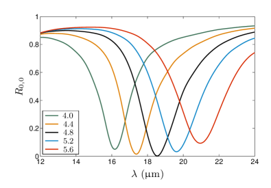
(a)  Simulations.

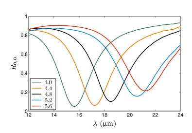
(b)  Experiments.

Figure 2: Reflexion spectrum at normal incidence in the specular order $R_{0,0}$ as a function of incident wavelength $\lambda$ for different values of the period $d$ (in $\mathrm{\SIUnitSymbolMicro m}$). (a): FEM simulations, (b): FTIR measurements.

Figure 2(a) shows the reflection spectra at normal incidence in the specular order for bi-gratings with different periods, calculated by the FEM formulation described in section II.1. These spectra show a clear resonant behavior in the region $12-$24\text{\,}\mathrm{\SIUnitSymbolMicro m}$$ with a large reflection dip. Increasing the period $d$ shifts this dip to larger wavelengths and broadens the resonance. It can also be noted that for $d=$4.8\text{\,}\mathrm{\SIUnitSymbolMicro m}$$, the reflection is almost zero at resonance. Since the transmission is negligible because the thickness of the bottom metal layer is nearly twice the skin depth of chromium in this spectral range, the incident power is nearly totally absorbed by the metamaterial at resonance and dissipated by Joule heating.
The measured reflection spectra of the fabricated samples are reported in Fig. 2(b) and show very good agreement with numerical simulations. For example for $d=$4.8\text{\,}\mathrm{\SIUnitSymbolMicro m}$$, both experimental and simulated reflection dips are located at $18.5\text{\,}\mathrm{\SIUnitSymbolMicro m}$, although experimentally, the reflection minimum is 10%, more than the 0.3% simulated value. For all samples, the disagreements originates from spectral broadening of the measured reflection, wich is mainly due to size dispersion on the rod diameter over the fabricated samples.

III.3 Influence of the periodicity: a pole-zero approach

To highlight the resonant properties of the studied MIM arrays, we report here a modal analysis of such structures. We solved numerically the spectral problem (3) as described in section II.2, with quasiperiodicity coefficients $\alpha=\beta=0$. Due to the symmetry of the problem in these conditions, we find two degenerate outgoing leaky modes (associated with poles of the complex reflection coefficient $r_{0,0}$) and two degenerate incoming leaky modes (associated with zeros of $r_{0,0}$). The degenerescence corresponds to eigenmodes with TE and TM polarization.

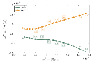
Figure 3: Location of pole (green squares) and zero (orange circles) in the complex plane as a function of $d$ (we only represented the pole and zero of the TE mode because of degeneracy). The values of $d$ are indicated in $\mathrm{\SIUnitSymbolMicro m}$, and the boxed values indicates the fabricated structures. The black dashed line represents the real axis.

Figure 3 shows the evolution of the pole and its associated zero in the complex $\omega$-plane as a function of $d$ (we only represented the pole and zero of the TE mode because of degeneracy). The real parts of the pole and of the zero are almost equal and shift to smaller frequencies as the period increases. For $d=$4.8\text{\,}\mathrm{\SIUnitSymbolMicro m}$$, the zero crosses the real axis, which means that the reflection is suppressed for a real incident frequency close to this zero. This is consistent with the previous observations from reflection spectra.

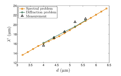
(a)  Resonant wavelength.

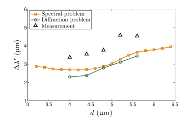
(b)  Spectral width.

Figure 4: Spectral parameters of the resonance as a function of the period $d$ obtained with different methods: extracted from calculated (green circles) and measured (black triangles) reflection spectra and extracted from the pole eigenfrequency (orange squares). (a): resonant wavelength, (b): spectral width.

We reported in Fig. 4 the values of the resonant wavelength and the spectral width of the resonances extracted from the calculated (green circles) and from measured (black triangles) reflection spectra as well as those derived from the pole eigenfrequencies (orange squares). As it can be seen in Fig. 4(a), the position of the resonance increases linearly with $d$, with the values calculated from simulated reflection spectra minima and from the spectral problem being in excellent agreement, which indicates that the resonant reflection dip stems from the excitation of the leaky mode associated with this eigenfrequency. In addition, experimental values well agree with the positions predicted by the two numerical approaches. Moreover, the spectral width of the dip increases with $d$ as can bee seen in Fig. 4(b). In that case the values obtained from the diffraction problem and from the spectral problem are in good agreement but slightly differs because the spectral width extracted from reflection spectra may be influenced by the presence of other modes whereas the linewidth associated with a leaky mode is valid for an isolated resonance. The experimental values are larger as said before but show a variation with $d$ similar to the calculated ones.

To highlight the physical mechanism responsible for these resonant total absorption (or equivalently suppressed reflection), we plotted in Fig. 5 the magnetic field associated with the TE outgoing quasimode for $d=$4.8\text{\,}\mathrm{\SIUnitSymbolMicro m}$$. The electric displacement represented by arrows is very strong with opposite directions in the rod and the metal layer, which creates a strong magnetic response (see colormap) confined in the silicon layer below the nanorod. Note that the nature of the resonance is not related to Fabry-Pérot type mechanism because the silicon layer is very thin ($<\lambda/30$), but rather to localized electric and magnetic dipoles Hao et al. (2010).

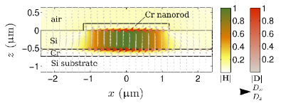
Figure 5: Field map of the TE outgoing leaky mode in the $Oxz$ plane for $d=$4.8\text{\,}\mathrm{\SIUnitSymbolMicro m}$$. The left colormap represents the norm of the magnetic field $\bm{H}$, the arrows represent the direction of the displacement current $\bm{D}$ and their colors (right colormap) and size are proportional to its intensity.

III.4 Angular tolerance

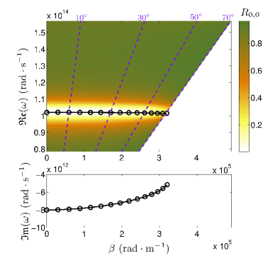
(a)  Simulations, TE.

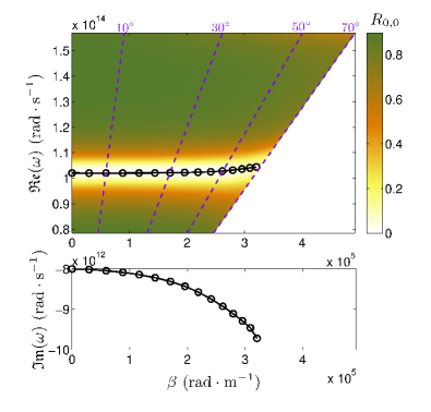
(b)  Simulations, TM.

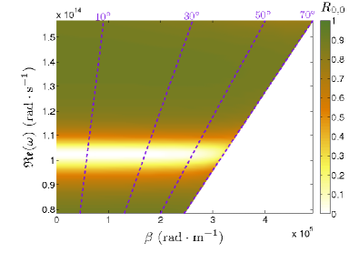
(c)  Simulations, unpolarized.

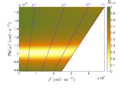
(d)  Experiments.

Figure 6: Influence of the incidence. Colormap : reflection spectrum in the specular order $R_{0,0}$ as a function of frequency $\omega$ and quasiperiodicity coefficient $\beta$ for $d=$4.8\text{\,}\mathrm{\SIUnitSymbolMicro m}$$. (a): simulations TE polarization, (b): simulations TM polarization , (c): simulations unpolarized, (d): FTIR measurements. In Figs. (a) and (b), the black circles indicate the real (top) and imaginary (bottom) parts of the eigenfrequency $\omega_{1}$ of the corresponding leaky mode as a function of $\beta$.

One of the key features of MIM arrays is the angular tolerance of the first order resonance, which is crucial for filtering applications. The colormap on Fig 6 shows the reflection spectrum as function of frequency $\omega$ and transverse wavenumber $\beta$ for $d=$4.8\text{\,}\mathrm{\SIUnitSymbolMicro m}$$. Figs. 6(a) and 6(b) are calculated values in TE and TM polarization respectively. We also plotted the evolution of the real part $\omega^{\prime}_{1}$ of the eigenfrequency $\omega_{1}$ associated with either TE or TM mode, the so-called dispersion diagram. In both cases the real part of the eigenfrequency remains almost constant, with a slight redshift (resp. blueshift) for TM (resp. TE) polarization at large angles and matches very well the position of the resonant reflection dip. As $\beta$ increases, the resonance sharpens in the TE case and broadens in the TM case. These observations are confirmed by the evolution of imaginary part $\omega^{\prime\prime}_{1}$ of eigenfrequencies (See bottom plot in Figs. 6(a) and 6(b)): because the real part $\omega^{\prime}$ is almost constant the quality factor of the resonance $Q=\omega^{\prime}/\Delta\omega=\omega^{\prime}_{1}/2\omega^{\prime\prime}_{1}$ increases (resp. decreases) for TE (resp. TM) polarization. To compare with experimental results of Fig. 6(d), we also plotted the calculated unpolarized case in Fig. 6(c). The agreement between simulations and measurements is excellent except a slight spectral broadening and higher minimum values for experimental results and demonstrates the angular tolerance up to $70\text{\,}\mathrm{\SIUnitSymbolDegree}$ of the fabricated filters.

III.5 Leaky mode excitation and reduced order model

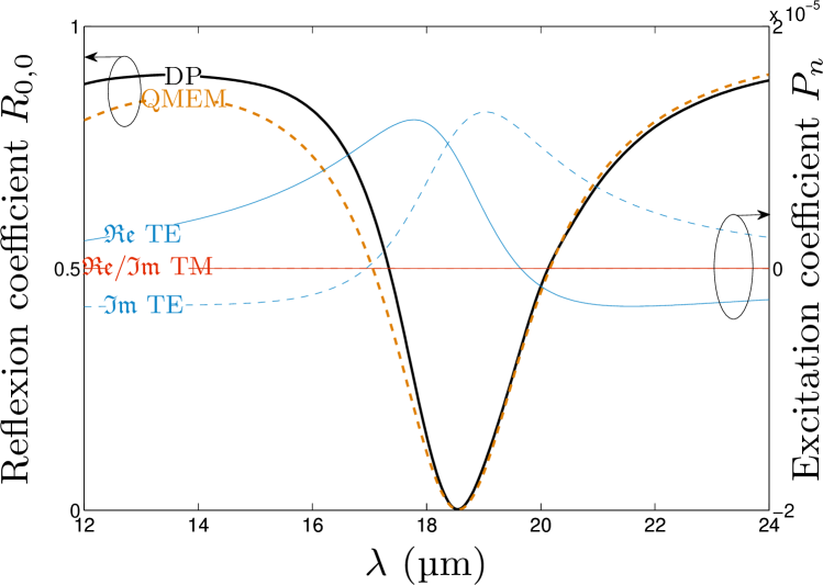
(a)  $\psi=0$ (TE)

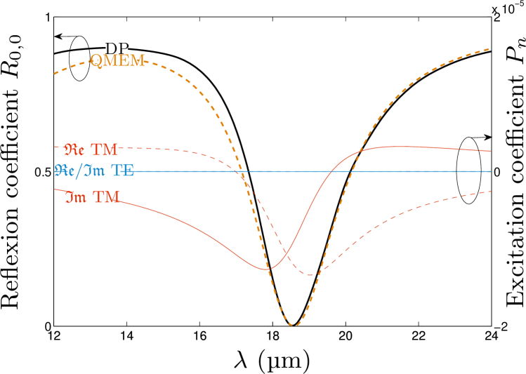
(b)  $\psi=\pi/2$ (TM)

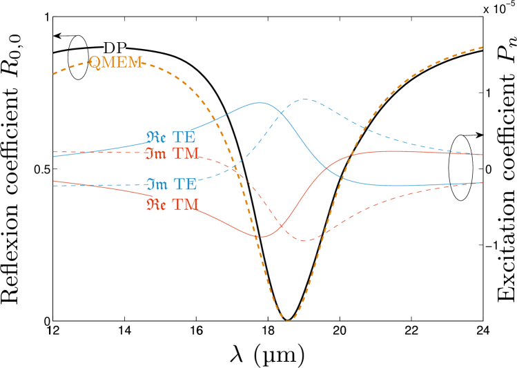
(c)  $\psi=\pi/4$

Figure 7: Excitation coefficients $P_{n}$ for the two degenerate modes (right ordinate, TE blue, TM red, real parts: solid line, imaginary part: dashed line) and reflection coefficient $R_{0,0}$ computed with full wave FEM diffraction problem (DP, black solid line) and with the QMEM with these two modes (orange dashed line).

Finally, we computed the diffracted field using Eq. (11) with the two leaky modes TE and TM. Because of the mode degeneracy, every linear combination of the two eigenmodes is also solution of Eq. (3) for the eigenvalue denoted $\omega_{1}=\omega^{\prime}_{1}+i\omega^{\prime\prime}_{1}$. We define the TE mode such that $J_{\rm{TE}}(\omega_{1}^{\prime},\psi_{\rm{TE}})=1$ and $J_{\rm{TE}}(\omega_{1}^{\prime},\psi_{\rm{TM}})=0$, where $\psi_{\rm{TE}}=0$ and $\psi_{\rm{TM}}=\pi/2$. The TM mode is then obtained by standard Gram-Schmidt orthogonalization procedure, and the two modes are finally normalized such that $K_{\rm{TE}}=K_{\rm{TM}}=1$.

The study of the coupling coefficients $P_{n}$ reveals the resonant nature of the interaction of a plane wave with the modes. On Fig. 7, we plot these coefficients as a function of wavelength for different polarization cases: (a) $\psi=0$ (TE), (b) $\psi=\pi/2$ (TM) and (c) $\psi=\pi/4$. The real (solid line) and imaginary (dashed line) parts of the excitation coefficients show strong variations around the resonant frequency in all cases. For $\psi=0$ (resp. $\psi=\pi/2$), only the TE (resp. TM) mode is excited while the value of $P_{n}$ for the TM (resp. TE) mode is negligible. For $\psi=\pi/4$ both modes participate equally to the resonant diffraction process as their coupling coefficients are equal in absolute value (opposite sign is arbitrarily set for display purpose). These observations illustrate the independence of the reflection dip with regards to polarization. We have also computed $R_{0,0}$ with the field reconstructed by the QMEM with only two leaky modes. The results (orange dashed line on Fig. 7) are in all cases in excellent agreement with full wave FEM simulations of the diffraction problem (DP, black solid line). This means that the diffractive properties of the structure are dominated by these two modes in the considered wavelength range. The small discrepancies at small wavelengths are attributed to other modes with higher resonant frequencies not taken into account in the reduced order model.

IV Conclusion

We have studied metamaterial based on MIM designed to serve as reflection bandcut filters in the thermal infrared spectral range. These structures shows quasi total absorption of light at the resonant wavelength that can be tuned by varying the lateral dimensions of the metallic nanorods grating. The reflection dip spectral position is also independent of incident angle up to $70\text{\,}\mathrm{\SIUnitSymbolDegree}$ and is not affected by the polarization state of the incident light. Our study provides an in depth modal analysis revealing the resonant nature of the interaction of light with leaky modes of the structure. We developed a quasimodal expansion method (QMEM) that allows us to compute coupling coefficients between a plane wave and the modes. This method leads to a reduced order model with two modes that fits very well full wave FEM diffraction problem simulations. Large area samples have been fabricated and FTIR measured reflection spectra are in good agreement with the different numerical approaches, demonstrating the potential practical application of those polarization independent and angular tolerant resonant filters. Although the filters studied here have been designed to work between $15$ and $22\text{\,}\mathrm{\SIUnitSymbolMicro m}$, the concepts studied here can be applied to higher frequency ranges (e.g. band III of the infrared between $7$ and $13\text{\,}\mathrm{\SIUnitSymbolMicro m}$) by scaling down the dimensions of the structures.

References

- Wood (1902) R. W. Wood, Proceedings of the Physical Society of London 18, 269 (1902).
- Hutley and Maystre (1976) M. Hutley and D. Maystre, Optics Communications 19, 431 (1976).
- Hessel and Oliner (1965) A. Hessel and A. A. Oliner, Appl. Opt. 4, 1275 (1965).
- Teperik et al. (2008) T. V. Teperik, F. J. Garcia de Abajo, A. G. Borisov, M. Abdelsalam, P. N. Bartlett, Y. Sugawara, and J. J. Baumberg, Nat Photon 2, 299 (2008).
- Landy et al. (2008) N. I. Landy, S. Sajuyigbe, J. J. Mock, D. R. Smith, and W. J. Padilla, Phys. Rev. Lett. 100, 207402 (2008).
- Bonod et al. (2008) N. Bonod, G. Tayeb, D. Maystre, S. Enoch, and E. Popov, Opt. Express 16, 15431 (2008).
- Tao et al. (2008) H. Tao, N. I. Landy, C. M. Bingham, X. Zhang, R. D. Averitt, and W. J. Padilla, Opt. Express 16, 7181 (2008).
- Hao et al. (2010) J. Hao, J. Wang, X. Liu, W. J. Padilla, L. Zhou, and M. Qiu, Applied Physics Letters 96, 251104 (2010).
- Liu et al. (2010) N. Liu, M. Mesch, T. Weiss, M. Hentschel, and H. Giessen, Nano Letters 10, 2342 (2010).
- Maier and Brückl (2009) T. Maier and H. Brückl, Opt. Lett. 34, 3012 (2009).
- Maier and Brueckl (2010) T. Maier and H. Brueckl, Opt. Lett. 35, 3766 (2010).
- Aydin et al. (2011) K. Aydin, V. E. Ferry, R. M. Briggs, and H. A. Atwater, Nat Commun 2, 517 (2011).
- Bouchon et al. (2012) P. Bouchon, C. Koechlin, F. Pardo, R. Haïdar, and J.-L. Pelouard, Opt. Lett. 37, 1038 (2012).
- Hao et al. (2011) J. Hao, L. Zhou, and M. Qiu, Phys. Rev. B 83, 165107 (2011).
- Popov et al. (1986) E. Popov, L. Mashev, and D. Maystre, Journal of Modern Optics 33, 607 (1986).
- Nevière et al. (1995) M. Nevière, E. Popov, and R. Reinisch, J. Opt. Soc. Am. A 12, 513 (1995).
- Tikhodeev et al. (2002) S. G. Tikhodeev, A. L. Yablonskii, E. A. Muljarov, N. A. Gippius, and T. Ishihara, Phys. Rev. B 66, 045102 (2002).
- Fehrembach and Sentenac (2003) A.-L. Fehrembach and A. Sentenac, J. Opt. Soc. Am. A 20, 481 (2003).
- Lalanne et al. (2006) P. Lalanne, J. P. Hugonin, and P. Chavel, J. Lightwave Technol. 24, 2442 (2006).
- Grigoriev et al. (2013) V. Grigoriev, S. Varault, G. Boudarham, B. Stout, J. Wenger, and N. Bonod, Phys. Rev. A 88, 063805 (2013).
- Fehrembach and Sentenac (2005) A. L. Fehrembach and A. Sentenac, Appl. Phys. Lett. 86, 121105 (2005).
- Sentenac and Fehrembach (2005) A. Sentenac and A.-L. Fehrembach, J. Opt. Soc. Am. A 22, 475 (2005).
- Ding and Magnusson (2004a) Y. Ding and R. Magnusson, Opt. Express 12, 5661 (2004a).
- Ding and Magnusson (2004b) Y. Ding and R. Magnusson, Opt. Lett. 29, 1135 (2004b).
- Ding and Magnusson (2004c) Y. Ding and R. Magnusson, Opt. Express 12, 1885 (2004c).
- Lovrinčić and Pucci (2009) R. Lovrinčić and A. Pucci, Phys. Rev. B 80, 205404 (2009).
- Palik (1991) E. D. Palik, Handbook of optical constants of solids (Academic Press, 1991).
- Macleod (2001) H. Macleod, Thin-film optical filters, 3rd ed. (Institute of Physics Pub., 2001).
- Demésy et al. (2009) G. Demésy, F. Zolla, A. Nicolet, and M. Commandré, Opt. Lett. 34, 2216 (2009).
- Demésy et al. (2007) G. Demésy, F. Zolla, A. Nicolet, M. Commandré, and C. Fossati, Opt. Express 15, 18089 (2007).
- Demésy et al. (2009) G. Demésy, F. Zolla, A. Nicolet, and M. Commandré, in Proceedings SPIE, Vol. 7353 (Prague, Czech Republic, 2009) p. 73530G.
- Schenk and Gärtner (2004) O. Schenk and K. Gärtner, Future Generation Computer Systems 20, 475 (2004).
- Ould Agha et al. (2008) Y. Ould Agha, F. Zolla, A. Nicolet, and S. Guenneau, COMPEL 27, 95 (2008).
- Popovic (2003) M. Popovic, in Integrated Photonics Research (Optical Society of America, 2003) p. ITuD4.
- Hein et al. (2004) S. Hein, T. Hohage, and W. Koch, J. Fluid Mech. 506, 255 (2004).
- Eliseev et al. (2005) M. V. Eliseev, A. G. Rozhnev, and A. B. Manenkov, J. Lightwave Technol. 23, 2586 (2005).
- Vial et al. (2014) B. Vial, F. Zolla, A. Nicolet, and M. Commandré, Submitted to Phys. Rev. A (2014).
- Note (1) Actually, the boundary conditions employed here are identical for both spectral problems since we use only real valued coefficents (homogeneous Neumann boundary condition and real quasiperiodicity constants and ).
- Hanson and Yakovlev (2002) G. Hanson and A. Yakovlev, Operator Theory for Electromagnetics: An Introduction (Springer, 2002).