Testing the rotating lighthouse model with the double pulsar system PSR J0737-3039A/B

Abstract

Each of the two pulsars in the double pulsar PSR J0737-3039A/B system exhibits not only the pulses emanating from itself, but also displays modulations near the pulse period of the other. Freire et al. (2009, MNRAS, 396, 1764) have put forward a technique using the modulation of B by A to determine the sense of rotation of pulsar A relative to its orbital motion, among other quantities. In this paper, we present another technique with the same purpose. While the Freire et al. approach analyzes pulse arrival times, ours instead uses periods or frequencies (their inverses), which can be experimentally determined via power spectral analysis similar to that used in pulsar searches. Our technique is based on the apparent change in spin period of a body when it is measured from an orbiting platform (the other pulsar), and is shown to be entirely analogous to the difference between the sidereal and solar spin period of the Earth (i.e., the sidereal and solar day). Two benefits of this approach are its conceptual and computational simplicity. The direct detection of spin with this technique will observationally validate the rotating lighthouse model of pulsar emission, while the detection of the relative directions of spin and orbital angular momenta has important evolutionary implications. Our technique can be used on other binary systems exhibiting mutually induced phenomena.

1 Introduction

The double pulsar system PSR J0737-3039A/B was discovered by Burgay et al. (2003) and Lyne et al. (2004). This system consists of a 22-ms pulsar (hereafter A) and a 2.8-s pulsar (hereafter B) with an orbital period of 2.4 hours. This discovery has provided a laboratory for the study of relativistic gravity and gravitational radiation (Kramer & Wex, 2009). The system has several strange features that challenge the current understanding of pulsars and provide an uncommon opportunity to improve pulsar theories. One of the most interesting properties is the observed modulation of each pulsar’s signal by the energy flux from the other, as evidenced by each pulsar’s modulation period being approximately equal to the other pulsar’s pulse period (McLaughlin et al., 2004a, b). Freire et al. (2009a) proposed a technique for analysing the arrival times of the pulsars’ pulses and their mutual modulations which could yield the sense of rotation of each pulsar with respect to its orbital motion, among other quantities. In this paper, a complementary technique is presented with the same objective, but using measured periods rather than arrival times. The principal benefit of our approach is that it is simpler and more intuitive. If the validity of either of these techniques is confirmed, not only will new insights be gained but also the correctness of the lighthouse model will be empirically assessed beyond dispute.

Table 1: Earth-Sun and double pulsar analogies. All quantities are defined as magnitudes.

Rotating object:	Earth $(\earth)$	Pulsar A
Orbital period, Mean orbital frequency	$P_{\rm orb}(\equiv$ year), $f_{\rm orb}$	$P_{\rm orb},f_{\rm orb}$
Instantaneous orbital frequency	$f_{\rm orb}(t)$	$f_{\rm orb}(t)$
Rotating object’s sidereal spin period, frequency	$P_{\earth,0}(\equiv$ sidereal day), $f_{\earth,0}$	$P_{\rm A,0},f_{\rm A,0}$
Rotating object’s spin period, frequency (measured at other body)	$P_{\earth\ \rm at\ \sun}(\equiv$solar day), $f_{\earth\ \rm at\ \sun}$	$P_{\rm A\ at\ B},f_{\rm A\ at\ B}$
$\equiv\$Modulation period, frequency at other body due to rotating object	$\equiv P_{\rm m\ at\ \sun\ due\ to\ \earth},$	$\equiv P_{\rm m\ at\ B\ due\ to\ A},$
	$f_{\rm m\ at\ \sun\ due\ to\ \earth}$	$f_{\rm m\ at\ B\ due\ to\ A}$

2 Determining the presence and sense of rotation of A, and analogies to the Earth-Sun system

Our method is identical in principle to the determination of the difference between two measurements of the Earth’s spin period – its sidereal and solar day. The difference between the two periods is caused by the kinematic effect of Earth’s rotation and revolution. Because the earth rotates and revolves in the same (“prograde”) sense, the solar day is about 4 min longer than the sidereal day. If the earth rotated in the opposite (“retrograde”) sense relative to its orbit, the solar day would be about 4 min shorter than the sidereal day. A similar relationship should be seen in the PSR J0737-3039A/B binary system if the lighthouse model is correct, where the apparent period of one pulsar’s pulses measured at the other pulsar – the other pulsar’s “modulation period” – will be longer or shorter than the first pulsar’s sidereal period if the first is a “lighthouse” rotating in the same or opposite direction as it is orbiting.

Although our technique can in principle be used to determine whether or not both A and B are spinning and the sense of such rotation with respect to their orbital motion, we focus only on determination of the spin of A in this and next sections, in order to avoid confusion. Then Earth’s sidereal day, $P_{\earth,0}$, is analogous to A’s sidereal rotation period, $P_{\rm A,0}$. Similarly, Earth’s solar day, $P_{\earth\ \rm at\ \sun}$, is analogous to the modulation period in B’s, signal, $P_{\rm m\ at\ B\ due\ to\ A}$. Table 1 further illustrates the analogies between the Earth-Sun system and the double pulsar system, in terms of the various periods and their corresponding frequencies $f=1/P$. In what follows, we will generally use spin and orbital frequencies instead of periods, because the frequency calculations are simpler.

To further understand the relationships among the rotation, revolution and modulation signals, consider the following suppositional extreme case. Assume that the spin periods of A and B are both equal to the orbital period and that both stars rotate in the same sense as their orbital motion. Then their emission signals will not modulate each other because each star can receive only steady energy fluxes from the other star. In any other case, it is clear that modulation of one pulsar’s signal by the other is possible, and that the period of modulation will be affected not only by the rotation period of the pulsar causing the modulation but also its orbital period and rotation sense.

From the analysis above, we have shown that as long as we can measure the modulation frequency of B’s signal, we can determine the presence and sense of rotation of A.

3 frequency determinations

When a radiotelescope points to the system PSR J0737-3039A/B, up to four periodicities may be received simultaneously; namely A’s and B’s direct and modulated signals. They will be intermingled at the radiotelescope since they are spatially indistinguishable at the solar system. In this section, we focus on the signals originating at A. (See Sec. 4 for a discussion of signals originating at B.)

3.1 Signal paths originating at A

Signals are observed from from pulsar A via two different paths: (1) the “direct beam” travelling directly from A to the solar system; and (2) the “two-legged” beam emitted by A that first impinges on B, thereby modulating B’s beam every time that A shines on B; with the modulated signal then travelling from B to the solar system. Consequently, the modulated signal encodes information concerning both B’s and A’s pulses.

Details of the orbital geometry are shown in Fig. 1. Note that it is the first leg of the two-legged path which provides the capability to distinguish the direction of A’s spin, if any; because it enables us to measure A’s pulse period with respect to a another vantage point (namely pulsar B’s), in addition to our own.

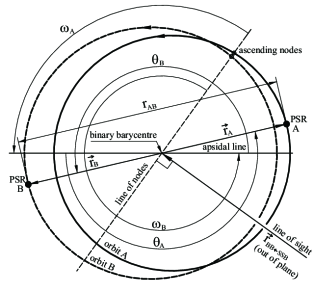
Figure 1: Orbits of PSRs A and B about the binary barycentre. The direct signal path discussed in the text is emitted from pulsar A antiparallel to the line of sight vector; while the “two-legged” signal path also starts at A but then travels to B before travelling antiparallel to the line of sight vector.

3.2 Frequency calculations

It will be adequate for our purposes to ignore kinematic modifications to source frequencies beyond order $v/c$, leaving only the first-order Doppler shift. The Doppler shift modifies $f_{\rm X,0}$, the emitted frequency of source ‘X’, leading to a received frequency $f_{\rm X,rcv}$ according to the following prescription:

$$f_{\rm X,rcv}=\left[1+\frac{\vec{\mathbf{v}}_{\rm X}\cdot\hat{\mathbf{r}}_{\rm X\leftarrow rcv}}{c}\right]^{-1}\times\ \ f_{\rm X,0}\ ,$$ (1)

where the dot-product projects the velocity of source ‘X’ with respect to receiver ‘rcv’ , $\vec{\mathbf{v}}_{\rm X}$, onto the receiver-to-source-‘X’ line-of-sight unit vector $\hat{\mathbf{r}}_{\rm X\leftarrow rcv}$, thereby yielding the “radial” (with respect to the receiver) velocity component. In what follows, source ‘X’ may be PSR A or PSR B, and ‘rcv’ may be located at the solar system barycentre, ssb; or even at PSR B (see below). In each such case, the subscripts will be replaced by appropriate symbols to denote the particular choices.

We define the “Doppler factor” D[X, rcv] solely for compactness of notation:

$${\mathbf{D}}[{\rm X,rcv}]\equiv\left[1+\frac{\vec{\mathbf{v}}_{\rm X}\cdot\hat{\mathbf{r}}_{\rm X\leftarrow rcv}}{c}\right]^{-1},$$ (2)

such that Eq. 1 becomes

$$f_{\rm X,rcv}={\mathbf{D}}[\rm X,rcv]\times f_{\rm X,0}.$$ (3)

(The two arguments of D denote the source and the receiver, respectively.)

Table 2: Magnitudes of frequencies $f(=1/P)$ on two signal paths for A’s emission.

Signal path 1: Direct beam from A to solar system barycentre (ssb)
Intrinsic spin frequency of A:		$f_{\rm A,0}$
Apparent spin frequency of A at ssb,
$f_{\rm 1,ssb}=f_{\rm A,ssb}$:		${\mathbf{D}}[{\rm A,ssb}]\times f_{\rm A,0}$
Signal path 2: Two-legged beam from A to B to solar system barycentre
	lighthouse model		other model
A’s rotation sense relative to orbit:	prograde	retrograde	none
Intrinsic modulation frequency of B,
$f_{\rm m\ at\ B\ due\ to\ A}$:	${\mathbf{D}}[{\rm A,B}]\times(f_{\rm A,0}-f_{\rm orb}(t))\$	${\mathbf{D}}[{\rm A,B}]\times(f_{\rm A,0}+f_{\rm orb}(t))\ ^{a}$	${\mathbf{D}}[{\rm A,B}]\times f_{\rm A,0}$
Apparent modulation frequency of
B at ssb, $f_{\rm 2,ssb}=f_{\rm m,ssb}$:	${\mathbf{D}}[{\rm B,ssb}]\times{\mathbf{D}}[{\rm A,B}]\times(f_{\rm A,0}-f_{\rm orb}(t))$	${\mathbf{D}}[{\rm B,ssb}]\times{\mathbf{D}}[{\rm A,B}]\times(f_{\rm A,0}+f_{\rm orb}(t))$	${\mathbf{D}}[{\rm B,ssb}]\times{\mathbf{D}}[{\rm A,B}]\times f_{\rm A,0}$

3.2.1 Radial velocity calculations

There are well-developed techniques for determining the radial velocity of an orbiting body X (the dot-product appearing in Eqs. 1 and 2) in terms of its orbital elements. Following Freire et al. (2001, 2009b), the radial (with respect to the receiver) velocity of object X, at any point in its orbit, is given by

$$\vec{\mathbf{v}}_{\rm X}\cdot\hat{\mathbf{r}}_{\rm X\leftarrow rcv}=\frac{2\pi}{P_{\rm orb}}\ \frac{a_{\rm X}\sin i}{\sqrt{1-e^{2}}}[\cos(\omega_{\rm X}+\theta(t))+e\cos\omega_{X}],$$ (4)

where $a_{\rm X}$ is the semimajor axis of the orbit of ‘X’, inclination $i$ is the angle between a vector normal to the orbital plane and $\hat{\mathbf{r}}_{\rm X\leftarrow obs},e$ is the orbital eccentricity, $\omega_{X}$ is the argument of periastron of X’s orbit, and true anomaly $\theta(t)$ is the polar angle of ‘X’ at emission time $t$, measured around the principal focus of its orbit, starting at periastron. Finally, in order relate all of these quantities explicitly to time, one must determine the value of $\theta(t)$ at a given emission time via the iterative “Kepler’s Equation” technique, as given in celestial mechanics texts [ e.g., Roy (2005) ]. Note also that $\omega_{X}$ is also a (slowly and essentially linearly-varying) function of $t$, due to a general relativistic phenomenon that is easily accounted for. Finally, for the special case of the relative orbit of PSR A about PSR B, Eq. 2 becomes

$${\mathbf{D}}[{\rm A,B}]=\left[1+\frac{\vec{\mathbf{v}}_{\rm rel,A}\cdot\hat{\mathbf{r}}_{\rm A\leftarrow B}}{c}\right]^{-1}=\left[1+\frac{\dot{r}_{{\rm rel,A}}}{c}\right]^{-1}$$

$$=\left[1+\frac{2\pi}{P_{\rm orb}}\ \frac{a_{\rm rel}\ e}{\ c\sqrt{1-e^{2}}}\sin\theta(t)\right]^{-1},$$ (5)

where $\vec{\mathbf{v}}_{{\rm rel,A}}$ and $\dot{r}_{{\rm rel,A}}$ are, for the relative orbit of PSR A about PSR B, the vector velocity and its radial (with respect to B) part, respectively.

3.2.2 Apparent frequencies at the solar system barycentre

In this section, we discuss the transformations necessary to find apparent frequencies of A’s two beams at a given time at the solar system barycentre, in terms of emission times, Doppler factors, intrinsic orbital and spin frequencies. Table 2 displays detailed expressions associated with these items.

The first (direct) beam from A: The intrinsic frequency of this beam, $f_{\rm A,0}$, will be Doppler-shifted upon receipt at the solar system barycentre due to A’s orbital velocity at the time of emission, yielding $f_{\rm 1,ssb}=f_{\rm A,ssb}={\mathbf{D}}[{\rm A,ssb}]\times f_{\rm A,0}$.

The second (“two-legged”) pulsed signal from A: This signal travels along two segments in sequence: first from A to B and then from B to the solar system barycentre. Some investigators (e.g., Freire et al. (2009a) ) suggest that this “signal” may consist of relativistic charged particles rather than photons, but either will behave similarly in our frequency-based analysis. (While the arrival-time model of Freire et al. (2009a) allows for a possible longitude offset between A’s radio and electromagnetic beams, this constant phase offset drops out of our frequency-based analysis.)

The first leg’s pulsed signal will be received and reemitted by B as a “modulation” with an apparent frequency in B’s frame of $f_{\rm m\ at\ B\ due\ to\ A}$. This frequency is modified from its intrinsic value $f_{\rm A,0}$, primarily by A’s orbital motion about B in a fashion analogous to the modification of Earth’s intrinsic spin frequency to its solar one, as described in Section 2. This requires that

$$f_{\rm m\ at\ B\ due\ to\ A}=\;\;\ \;\;\ \;\;\ \;\;\;\;\ \;\;\ \;\;\ \;\;\;\;\ \;\;\ \;\;\ \;\;\;\;\ \;\;\;\;\;$$ (6)

$${\mathbf{D}}[{\rm A,B}]\times\begin{cases}(f_{\rm A,0}-f_{\rm orb}(t)\ )&\text{prograde spin,}\\ (f_{\rm A,0}+f_{\rm orb}(t)\ )&\text{retrograde spin,}\\ \ f_{\rm A,0}&\text{pulsation (no}\\ &\text{\ \ \ \ \ \ \ \ \ \ \ \ spin);}\\ \end{cases}$$

as summarized in Table 2.

It is easy to show that this kinematic consequence of the lighthouse model leads to exactly one fewer (prograde case) or one extra (retrograde case) pulse from PSR A per orbital period, compared with the no-spin number. The former case is closely analogous to the (prograde) Earth - Sun system, where there is one fewer solar day than sidereal days per Earth year.

Eq. 6 would have a particularly simple form if the orbit were circular, both because $f_{\rm orb}$ could be treated as a constant and because the Doppler shift function ${\mathbf{D}}[{\rm A,B}]\equiv 1$ in this case. The difference between the exact, elliptical orbit expression given in Eq. 6 and this fictitious, circular-orbit expression is intimately related to the difference between the apparent and mean spin frequencies of the Earth with respect to the Sun which leads to a time-varying difference between apparent and mean solar time, dubbed the “Equation of Time” (Seidelmann, 1992).

The pulse train on the second portion of this trajectory, leaving B with a frequency $f_{\rm m\ at\ B\ due\ to\ A}$ of Eq. 6, will be Doppler shifted upon its reception at the solar system barycentre due B’s orbital motion, leading to modulation frequency

$$f_{\rm 2,ssb}=f_{\rm m,ssb}={\mathbf{D}}[{\rm B,ssb}]\times f_{\rm m\ at\ B\ due\ to\ A}\;\;\;\;\;\;\;\;\;\;\;\;\;\;\;\;\;\;\;\;\;\;\;\;$$ (6a)

$$={\mathbf{D}}[{\rm B,ssb}]\times{\mathbf{D}}[{\rm A,B}]\times\begin{cases}(f_{\rm A,0}-f_{\rm orb}(t)\ )&\text{prograde spin,}\\ (f_{\rm A,0}+f_{\rm orb}(t)\ )&\text{retrograde spin,}\\ \ f_{\rm A,0}&\text{pulsation (no}\\ &\text{\ \ \ \ \ \ \ \ \ \ \ \ spin).}\\ \end{cases}$$ (6b)

3.3 Spin-A-Induced Offsets in B’s modulated signal

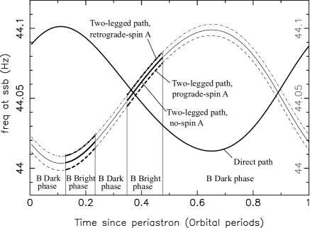
Figure 2: Apparent frequencies of direct and two-legged pulses originating from A, at the solar system barycentre, as a function of time for MJD 54155. The frequency of the direct path (A $\rightarrow$ ssb ), $f_{\rm 1,ssb}$, is the isolated curve, while the three possible values of the modulation pulse train frequency, $f_{\rm m,ssb}=f_{\rm 2,ssb}$, of the “two-legged” path (A $\rightarrow$ B $\rightarrow$ ssb) are depicted (with a $40\times$ exaggeration of their offsets from the middle, no-spin curve) as three closely-spaced curves. Vertical lines delimit the parts of the orbit where B is visible (labelled “Bright phase”) or invisible (labelled “Dark phase”). Since the two-legged path is actually detected as a modulation of B’s signal, the two-legged path could never be observed during B’s “dark phases,” so the two-legged curves are shown as fainter lines at these phases. B’s modulation was actually only detected in a small region of the first bright phase, although we believe it would be worthwhile to use our techniques to search for modulations throughout both bright phases. A similar,but mirror- image, set of curves centered near 0.36 Hz would be created if a similar pair of beams originates at PSR B (see §4).

The essence of our test for the rotation of A is contained in Eqs. 6, since the sense or even the existence of A’s spin will select one of the three versions of Eqs. 6b for the value of B’s drifting- subpulse-like modulation frequency. Hence the modulation has only three allowed values at a given orbital phase. Fig. 2 illustrates the direct-path and the three possible two-legged-path pulse train frequencies of the beams from A at the solar system barycentre as a function of time, with the offset of the two extreme values from the central, no-spin, curve for the two-legged beam exaggerated by a factor of forty.

Indeed, B’s pulses are clearly modulated by A’s emission (McLaughlin et al., 2004a). Therefore, as long as the data are sufficiently ample, the modulation frequency $f_{\rm m,ssb}$ should be obtainable with enough precision to distinguish among the three possibilities.

As can be ascertained from Eqs. 6b, the mean frequency offset at the ssb between each of the three possible two-legged paths, is

$$|\Delta f_{\rm 2,ssb}|=|\Delta f_{\rm m,ssb}|={\bf{D}}[{\rm B,ssb}]\times f_{\rm orb},$$ (7)

while the mean fractional offset $\delta$ is³:

$$\delta=\frac{|\Delta f_{\rm 2,ssb}|}{f_{\rm 2,ssb,no-spin}}=\frac{|\Delta f_{\rm m,ssb}|}{f_{\rm m,ssb,no-spin}}=\frac{{\bf{D}}[{\rm B,ssb}]\times f_{\rm orb}}{{\mathbf{D}}[{\rm B,ssb}]\times f_{\rm A,0}}$$

$$=\frac{f_{\rm orb}}{f_{\rm A,0}}.$$ (8)

The value of $\delta$ is only $0.00026\%$ [using $f_{\rm orb}=1/(8834.535$ s) and $f_{\rm 0,A}=44.0540694$ Hz (Kramer et al., 2006)]. While the three possible values of $f_{\rm m,ssb}$ are thus quite similar, we note that they are precisely calculable via Eqs. (6b), as illustrated in Fig. 2. The next section details an algorithm for determining the presence and sense of rotation of A from a real data set, by finding which of the three modulation frequencies best matches the data.

3.4 The algorithm

The results of the above sections derive and illustrate the three possible values of the ssb modulation frequency at any given orbital phase. However, these frequencies vary around the orbit due to Doppler shifts and orbital ellipticity, thereby rendering frequency searches difficult without special techniques. We discuss such techniques below.

Consider the observed, sampled (though incompletely) $k^{\rm th}$ intensity $I[k]$, measured at solar system barycentric time $t[k]$:

$$t[k]=t_{0}+\frac{k}{f_{\rm s}},$$ (9)

where $t_{0}$ is the ssb time of sample zero and $f_{\rm s}$ is the sampling frequency.

Full power spectral analyses could be employed on chunks of this time series whose durations are short enough to avoid significant spectral smearing due to Doppler shifts and orbital ellipticity. The highest-amplitude channel of the power spectrum near the expected modulation frequency could then be defined as the best estimate of the modulation frequency for a given chunk; and its value could then be compared with each of the three values of $f_{\rm m}$ predicted for that chunk by Eqs. 6b, thereby determining the presence and sense of rotation of A. However, since the three expected values are so similar, it would be difficult to distinguish among them in a relatively short and noisy chunk.

Therefore, it would be helpful to eliminate the Doppler and elliptical-orbit smearing of the modulation frequency around the orbit and beyond, in order to employ much longer data sets. Here we illustrate an algorithm to resample the full extant data set in order to “freeze” the desired modulation at a constant frequency, whose value can be determined via Fourier analysis of all the data at once. This procedure will result in much greater spectral resolution and signal-to-noise. The process is similar to procedures used in frequency-based searches of time series data for unknown binary pulsars, wherein the Doppler shifts due to putative orbital motion are eliminated via resampling of the data (e.g., Allen et al. (2013)). However, while unknown binary searches require resampling the data with multiple trial sets of parameters spanning an enormous search space, our procedure requires only one parameter set for each of the three possible rotational states, all of which are well-determined. In order to resample the data, we first calculate times $t_{\rm B}[k]$ and $t_{\rm A}[k]$, the times at B and A corresponding to ssb time $t[k]$ for the two-legged path from A to B to the ssb that is responsible for the drifting-subpulse-like modulation. Then we derive an expression for the phase of the modulation at B, taking elliptical orbital motion into account. Finally, we show how to determine the presence and nature of A’s spin by searching for periodicities in this modulation phase space.

3.4.1 Freezing the frequency of B’s pulses

First, we calculate $t_{\rm B}[k]$, the time of the $k^{th}$ sample measured at B, by correcting for B’s propagation contributions along the second leg, the path from B to the ssb:

$$t_{B}[k]=t[k]-\frac{L}{c}-\frac{z_{\rm B}}{c}=t_{0}+\frac{k}{f_{\rm s}}-\frac{L}{c}-\frac{z_{\rm B}}{c};$$ (10)

with $L$ the distance between the ssb and binary barycentre bb; and $z_{\rm B}$, the projection of the position of B with respect to the bb, $\vec{\mathbf{r}}_{\rm B}$, onto the line of sight $\hat{\mathbf{r}}_{\rm bb\leftarrow ssb}$:

$$z_{\rm B}\equiv\hat{\mathbf{r}}_{\rm bb\leftarrow ssb}\cdot\vec{\mathbf{r}}_{\rm B}=\frac{a_{\rm B}\sin i\ (1-e^{2})\sin(\omega_{\rm B}+\theta)}{c\ (1+e\cos\theta)}.$$ (11)

[See Sec. 3.2.1 for additional definitions, and Roy (2005) for a derivation.]

Eq. 10 can be used to transform $I[k]$, the intensity data sampled at the ssb, into a resampled space where the previously time-variable Doppler shift $\mathbf{D}[\rm B,ssb]$ caused by B’s orbital motion is removed. In this new space, the pulses from B will yield a fixed power spectral peak at $f_{B,0}$. Indeed, it is by this very technique that survey data are resampled in an effort to search for a binary pulsar of given orbital properties [e.g., Allen et al. (2013)] (in this case, properties matching B’s).

3.4.2 Freezing the frequency of the modulation

In order to freeze frequency of the the modulation occuring when A’s pulses interact with B, we must also calculate $t_{\rm A}[k]$, the time of the $k^{th}$ sample measured at A, by correcting additionally for propagation time $|d_{\rm AB}|/c$ along the path from A to B:

$$t_{A}[k]=t_{B}[k]-\frac{|d_{\rm AB}|}{c}=t_{0}+\frac{k}{f_{s}}-\frac{L}{c}-\frac{z_{\rm B}}{c}-\frac{|d_{\rm AB}|}{c},$$ (12)

with [see also Freire et al. (2009a)]:

$$\frac{|d_{\rm AB}|}{c}\approx\frac{|r_{\rm AB}|}{c}+\frac{dr_{\rm AB}}{dt}\Delta t_{\rm AB}=\frac{|r_{\rm AB}|}{c}(1+\frac{dr_{\rm AB}}{dt}),$$ (13)

where $|r_{\rm AB}|$ is the instantaneous separation between the two pulsars.

Eq. 12 implicitly eliminates the Doppler factors $\mathbf{D}[\rm B,ssb]$ and $\mathbf{D}[\rm A,B]$ in Eq. 6b caused by both pulsars’ radial motions along the two-legged path.

Now let us more carefully specify the (“unprime”) sidereal reference frame centred on A as one whose x-axis points from A to B’s position at periastron, and whose y-axis points in the direction of B’s motion at periastron. A is pulsing, or else spinning in a prograde or retrograde manner with respect to B’s revolution, all at a rate whose magnitude is $f_{\rm A,0}$ (cf. Table 1), measured in this unprime frame.

Therefore, the rotational or pulsational phase of A in the unprime, sidereal frame centred on A would be essentially⁵ strictly proportional to $t_{\rm A}:$

$$\Phi_{\rm A,0}[k]=\begin{cases}+2\pi f_{\rm A,0}\ t_{\rm A}[k]&\text{prograde spin.}\\ -2\pi f_{\rm A,0}\ t_{\rm A}[k]&\text{retrograde spin.}\\ \ \ 2\pi f_{\rm A,0}\ t_{\rm A}[k]&\text{pulsation (no spin).}\end{cases}$$ (14)

While $f_{A,0}$ is the sidereal frequency of A’s pulsations or rotations, it is not necessarily the frequency of A’s signal’s interception and modulation of B (i.e., it is not necessarily equal to the modulation frequency). Specifically, if A emits a rotating lighthouse beam, a correction must be made due to B’s orbital motion. (Conversely, if A is instead pulsating, no such correction is necessary because the pulsation is presumed to be emitted simultaneously in all directions.

In order to correct for orbital motion in the case of a rotating lighthouse beam, consider a second (“prime”) two-dimensional coordinate system lying in the orbital plane and centred on A, whose axes {x’,y’}, rotate (nonuniformly, due to the elliptical orbit) such that its x’-axis points from A toward B’s location at time $t_{\rm B}[k]$. The phase angle between the two coordinate systems (e.g., between the x- and x’-axes) is just the true anomaly $\theta(t_{\rm B}[k]$ (cf. Sec. 3.2.1).

The drifting-subpulse-like modulations, which are created whenever A’s emission intercepts B, occur at intervals separated by exactly one rotation or pulsation of A in the prime frame. Therefore, we can write an expression for the corresponding “modulation phase” $\Phi_{\rm m\ at\ B\ due\ to\ A}[k]$, which is just the rotational or pulsational phase of A in the prime frame:

$$\Phi_{\rm m\ at\ B\ due\ to\ A}[k]=\;\;\;\;\;\;\;\;\;\;\;\;\;\;\;\;\;\;\;\;\;\;\;\;\;\;\;\;\;\;\;\;\;\;\;\;\;\;\;\;\;\;\;\;$$

$$\begin{cases}+2\pi f_{\rm A,0}\ t_{\rm A}[k]-\theta(t_{B}[k])&\text{prograde spin,}\\ -2\pi f_{\rm A,0}\ t_{\rm A}[k]-\theta(t_{B}[k])&\text{retrograde spin,}\\ +2\pi f_{\rm A,0}\ t_{\rm A}[k]&\text{pulsation (no spin).}\end{cases}$$ (15)

The modulations now occur at phase intervals of $\Delta\Phi_{\rm m\ at\ B\ due\ to\ A}[k]=2\pi j$, with $j$ any positive integer. In this fashion, we have achieved our ultimate goal of “freezing” the modulations at a fixed periodicity in this transformed space, even in the presence of ellipticity-induced, time-variable orbital frequencies.

An observer can distinguish only the magnitude of the modulation phase, $|\Phi_{\rm m\ at\ B\ due\ to\ A}[k]|$, with

$$|\Phi_{\rm m\ at\ B\ due\ to\ A}[k]|_{s}=2\pi f_{\rm A,0}\ t_{\rm A}[k]-s\ \theta(t_{B}[k]),$$ (16)

where A’s spin state $s=\{+1,-1,\ 0\}$ for {prograde spin, retrograde spin, no spin but pulsation}, respectively. (Note that the right side of Eq. 16 will always be positive, as desired, since $f_{\rm A,0}>>d\theta/dt$.)

3.4.3 Determining A’s spin state s from observations

We have expressed the modulation phase magnitude at B, of the $k^{th}$ sample for each of the three possible spin states in Eq 16. We show below that this enables us to measure the modulation frequency at B via a periodicity search, thereby determining A’s true spin state.

In order to search for modulation periodicities over a range of frequencies, we will now represent the magnitude of A’s sidereal rotation period by a generalized variable $f_{\rm A,trial}$, whose value will be allowed to vary slightly about its known value:

$$f_{\rm A,trial}=zf_{\rm A,0},$$ (17)

where the frequency search factor $z\approx 1$. Then for each chosen $z$ and $s=\{+1,-1,0\}$, the modulation phase magnitude at B of the $k^{th}$ ssb sample is

$$|\Phi_{\rm m\ at\ B\ due\ to\ A}[k,z]|_{s}=2\pi\ (z\ f_{\rm A,0})\ t_{\rm A}[k]-s\ \theta(t_{B}[k])$$ (18)

We can now test for the presence of a modulation periodicity due to one of the three possible spin states, by doing a periodicity search in the vicinity of each such state in modulation-phase space. We associate the relevant modulation phase factor for a given state $s$, with each ssb-sampled intensity $I[k]$, and prepare a Fourier power spectrum of the product. The resulting quantity $P_{\rm n}(zf_{\rm A,0})_{s}$, the power in the $n^{th}$ harmonic of the modulation corresponding to A’s trial spin frequency $zf_{\rm A,0}$ and spin state $s$, is given by

$$P_{\rm n}(zf_{\rm A,0})_{s}=\left|\sum_{k}I[k]\;\exp{(-i\ n\ |\Phi_{\rm m\ at\ B\ due\ to\ A}[k,z]|_{s})}\right|^{2},$$ (19)

where $k$ can extend over any subset of the full ssb-sampled dataset.

The true spin state will then be manifested as a sharp peak in one of the three power spectra at the frequency corresponding to $z\equiv 1$ and its harmonics, while the power spectra generated for the other two putative spin states will exhibit no such peaks at the expected frequency and its harmonics. If necessary, the sought-after signal can be further enhanced by the process of harmonic summing, which is a well-established pulsar search technique.

The theoretical framework applied here can be further verified with a few additional observational procedures. For example, since the modulation of B’s pulses can occur only at those orbital phases where B’s pulses are present (denoted “bright phases” in Fig. 2), the sought-after modulation periodicity must also be visible only at those phases as well. [Indeed, the modulation phenomenon is only directly visible near the beginning of the first bright phase (McLaughlin et al., 2004a), although we believe it is worth deploying our technique with multiple trials on data from a wide range of bright phases.] Conversely, while the pulses arriving directly from A are observable at all orbital phases, the above procedures should filter out their presence in the resampled data.This ability to filter for the direct signal is key, especially if a pulsation (no spin) result appears. The success of the filtering out of the direct ray from A can itself be assessed by using our technique only on the (B-) dark phases, where only the direct A ray is emitted.

4 An alternative: Determining the presence and sense of rotation of B

An analysis of the apparent pulse train frequencies on the two equivalent paths from PSR B to the ssb (rather than the earlier case of paths originating at A) leads to identical expressions as above, except with subscripts “A” and “B” interchanged.

Indeed, McLaughlin et al. (2004b) and Breton et al. (2012) show that A’s pulses are modulated by B. However, the modulation has so far only been detected during the short (partial!) eclipse of A by B. Unfortunately, this modulation signal cannot be used to determine B’s rotation sense, because it arises from a different mechanism and hence the signal relationships differ from those derived above.

If A’s signal modulation by B can also be found in the non-eclipse phase, B’s rotation sense may be determined more easily than A’s. In this case, with $f_{\rm 0,B}=0.360560355$ Hz (Kramer et al., 2006), the equivalent mean fractional frequency offset distinguishing the three possible spin states of B is a much larger $0.031\%$. The data segments corresponding to the eclipse phases should be discarded in the analysis in order to avoid contamination from modulation originating by a different mechanism. While B’s radio signal disappeared in 2008 due to relativistic precession of the spin axis (Perera et al., 2010), it is possible that its spinning magnetosphere could still modulate A’s pulses. In addition, B’s beam should eventually precess back into our line of sight. Moreover, it may be worth using our techniques to investigate whether A’s signal is modulated by B in the non-eclipse phase, although it is unlikely for B to modulate A’s emission in the same way that A does B because the spindown power, which is proportional to $f\times\dot{f}$, is much less for B than for A (Kramer & Wex, 2009).

5 Conclusion

McLaughlin et al. (2004a) presented a modulation pattern similar to drifting subpulses in the signal of PSR B, but with a frequency of 44 Hz, close to the pulse frequency of PSR A. The presence and sense of rotation of A is encoded in the observed modulation pattern, and can be revealed through an arrival-time-based analysis (Freire et al., 2009a) or the frequency-based analysis presented above. Our procedure offers the benefits of relative conceptual simplicity and close analogy with familiar phenomena in the Earth-Sun system. We present a frequency-based procedure, building upon that used in binary pulsar search software, to distinguish among direct, retrograde, or no rotation of PSR A by searching synchronously for one of the three possible modulation signals over the full span of available data.

Although the lighthouse model has been widely accepted, there has nevertheless been no direct observational evidence in its support up to this time. A strength of our technique is its ability to provide such a test, empirically supporting or refuting the model.

Ferdman et al. (2013) have shown that A’s spin and orbital axes are aligned to within $3\degr$, but they have no direct means of distinguishing parallel from antiparallel alignment. By assuming parallel alignment, they are able to conclude that the second supernova, which created B, was relatively symmetric. Therefore the presence and sense of the rotation, as revealed by this analysis, will further test their and others’ (e.g., Kramer & Stairs (2008); Farr et al. (2011)) evolutionary scenarios.

While McLaughlin et al. (2004b) also found that A’s signal is modulated at B’s frequency near A’s eclipse, the mechanism is different and not dependent on B’s rotation. If, however, the modulation is observed in the future away from eclipse, it will provide an easier test for B’s rotation than does the approach delineated above for A.

Our analysis can also be used on other binary systems discovered to possess phenomena caused by mutual interactions.

References

- Allen et al. (2013) Allen, B., Knispel, B., Cordes, J. M., et al. 2013, APJ, 773, 91
- Breton et al. (2012) Breton, R. P., Kaspi, V. M., McLaughlin, M. A., et al. 2012, APJ, 747, 89
- Burgay et al. (2003) Burgay M. et al., 2003, Nature, 426, 531
- Farr et al. (2011) Farr, W. M., Kremer, K., Lyutikov, M., & Kalogera, V. 2011, APJ, 742, 81
- Ferdman et al. (2013) Ferdman, R. D., Stairs, I. H., Kramer, M., et al. 2013, APJ, 767, 85
- Freire et al. (2001) Freire, P. C., Kramer, M., & Lyne, A. G., 2001, MNRAS, 322, 885
- Freire et al. (2009a) Freire P. C. C. et al., 2009a, MNRAS, 396, 1764
- Freire et al. (2009b) Freire, P. C., Kramer, M., & Lyne, A. G. 2009b, MNRAS, 395, 1775
- Kramer et al. (2006) Kramer, M., Stairs, I. H., Manchester, R. N., et al., 2006, Science, 314, 97
- Kramer & Stairs (2008) Kramer, M., & Stairs, I. H. 2008, ARAA, 46, 541
- Kramer & Wex (2009) Kramer, M., & Wex, N., 2009, Classical and Quantum Gravity, 26, 073001
- Lyne et al. (2004) Lyne A.G. et al., 2004, Science, 303, 1153
- McLaughlin et al. (2004a) McLaughlin M. A. et al., 2004a, ApJ, 613, L57
- McLaughlin et al. (2004b) McLaughlin M. A. et al., 2004b, ApJ, 616, L131
- Perera et al. (2010) Perera, B. B. P., McLaughlin, M. A., Kramer, M., et al., 2010, APJ, 721, 1193
- Roy (2005) Roy, A. E. 2005, Orbital Motion, 4th ed. Bristol (UK): Institute of Physics Publishing.
- Seidelmann (1992) Seidelmann, P. K. 1992, Explanatory Supplement to the Astronomical Almanac, University Science Books.