Wrapping probabilities for Potts spin clusters on a torus

Abstract

In this work we obtain wrapping probabilities for Ising spin clusters on a torus. We use the analogy with the tricritical point of a Potts model with dilution. The formula obtained are tested against numerical simulation. We also provide closed form for the wrapping probabilities of cross clusters on untwisted tori.

Introduction

In the study of the critical properties of the Potts model, it was soon remarked that rewriting the model in terms of clusters was very enlightening [1, 2]. Indeed, the Fortuin-Kasteleyn (FK) clusters or droplets, obtained by casting the Potts partition function into a random cluster partition function, contain all the critical properties of the model and in particular are ruled by the same critical exponents. However, these are not the clusters one would observe in an experimental realisation of the Potts model, in this case one can only see the clusters formed by connected spins sharing the same value (spin clusters). In two dimensions both type of clusters undergo a continuous percolation transition at the critical temperature but a measure of the fractal dimensions of FK and spin clusters quickly convinces that the two types of clusters possess different critical exponents [3]. From a theoretical point of view there is then the question of the origin of this set of exponents ruling the properties of spin clusters. A clear answer can be given for the $Q=2$ states Potts model, i. e. the Ising model. In [2] it was shown that the Ising Hamiltonian can be rewritten as a diluted Potts model with $Q^{\prime}=1$ state. This enabled the computation of the Ising spin clusters exponents [4]. Unfortunately no such mapping exists for other Potts models. It was nonetheless conjectured in [5] that the exponents for spin clusters can be obtained by a similar mapping to a diluted Potts model with a different number of states at its tricritical point. This conjecture gives exponents compatible with numerical estimates [6, 7, 8] and there is little doubt that those are exact even though a rigorous proof is still lacking. The situation was thought to be more or less under control until recent works showed that a naive analytic continuation from the critical branch sometimes fails to give the correct results for some spin clusters properties. Even though no problem is encountered at the level of dimensions, a naive continuation is not able to explain the connectivity constants appearing in bulk three-point connectivity [9] and the corner contribution to cluster number [10]. It is thus very interesting to further study the properties of spin clusters to understand what can and cannot be obtained from an analytic continuation.

In percolation theory, it is a basic fact that below the percolation threshold no infinite cluster exists and that above there exists one with probability one [11]. At the percolation threshold, an important question for finite-size systems is whether a cluster spanning the whole system is present or in other words: what is the crossing probability of a percolation cluster for a given system? The study of crossing probabilities has a long history and a landmark in this topic is due to Cardy and his eponymous formula [12]. This formula gives the probability of left-right crossing of an incipient spanning cluster at the critical percolation threshold on a rectangle. This probability depends only upon the aspect ratio $r$ of the rectangle and can be expressed in terms of hypergeometric functions. At the same time Langlands et al. [13] tested numerically the universality of crossing probabilities in different setups. Since then a number of percolation probabilities have been studied either for percolation [14, 15, 16] or other models [17, 18, 19, 20]. One aspect that is particularly interesting is that although Cardy and others found those formulas using conformal field theory (CFT), i. e. in a non rigorous way mathematically speaking, rigorous tools have been developed which can be used to tackle those systems. Schramm introduced the stochastic Loewner evolution (SLE) [21] which describes numerous physically occurring curves (see [22] with Lawler and Werner e.g.). In a slightly different line of research Smirnov proved rigorously Cardy’s formula and the existence of a conformal scaling limit of the percolation critical point for site percolation on the triangular lattice [23].

As a generalisation of the case of simply connected surfaces, Langlands et al. introduced the notion of crossing probabilities on compact Riemann surfaces [24]. For percolation on a compact Riemann surface S, one can consider the topological space $X_{s}$ generated by a given configuration $s$ and the homomorphism $\phi:H_{1}(X_{s})\to H_{1}(S)$ from the first homology group of $X_{s}$ to that of $S$. The probability $\pi_{G}$ that a configuration $X_{s}$ contains in its image by $\phi$ a subgroup $G\subset H_{1}(S)$ is:

$$\pi_{G}=\frac{Z_{G}}{Z}$$ (1)

where $Z$ is the total partition function of the model considered and $Z_{G}$ the partition function restricted to the configurations generating $G$ by $\phi$. Among other cases Langlands et al. studied numerically those probabilities for percolation on a torus. Shortly after they were derived analytically for percolation by Pinson [14] building on the work of Di Francesco et al. [25]. Arguin [26] then extended the work of Pinson to the case of FK clusters of the $Q$ states Potts model for $Q\in[1,4]$. He was also able to derive closed forms in terms of Jacobi $\theta$ functions in the case of percolation ($Q=1$) and Ising FK clusters ($Q=2$) and supported his formula for integer values of $Q$ with simulations. In [27] it was checked numerically that the formula obtained by Arguin is also valid for real values of $Q$.

In the present work we further generalise the derivation of wrapping probabilities of FK clusters by Arguin to the case of Potts spin clusters. In the present work only the Ising model is treated. In this case a closed form in terms of Jacobi $\theta$ function is obtained and checked numerically. Even though other cases (mainly the 3-Potts model) are not treated explicity in this work it is expected that the arguments developped for the Ising spin clusters can be generalized to other cases. This work was motivated by the study of the appearance of long-lived stripe states in the Ising model after a quench from $T=T_{c}$ to $T=0$ with various boundary conditions [28]. When periodic boundary condition are applied, the system has the topology of a torus and wrapping probabilities of spin clusters are relevant to explain the appearance of long-lived stripe states [29, 30]. We also present expressions for the probabilities of cross-shaped FK and spin clusters for the Ising model on untwisted tori. The article is divided as follows: we further discuss FK and spin clusters, present how wrapping probabilities can be computed, show the derivation for Ising spin clusters and check it numerically and finally we provide expressions for cross-shaped clusters.

1 Potts model and spin clusters

In the following we study the ferromagnetic Potts model whose Hamiltonian is written as:

$${\cal H}=-J\sum_{\langle ij\rangle}\delta_{S_{i}S_{j}}\;,$$ (2)

where the sum is over all nearest neighbors pairs of spins of a $d$-dimensional system, $J>0$ and $\delta$ the Kronecker delta and $S_{i}$ the spin at site $i$ taking integer values in $[1,Q]$. The $Q\to 1$ limit of this model is known to correspond to percolation. This model undergoes a magnetic phase transition at the inverse temperature $\beta_{c}=1/T_{c}$ and this transition is continuous for $Q\leq Q_{c}(d)$. For $d=2$, $Q_{c}(2)=4$ and $\beta_{c}=\ln(1+\sqrt{Q})$ for the square lattice [6].

In the study of the Potts model two types of clusters emerge: the FK clusters and the same spin clusters. The FK clusters appear naturally when the Potts partition function is rewritten in the form of the random cluster model [1]. The construction of FK clusters is simple, edges between spins with the same value are open with probability $p=1-e^{-\beta J}$ and edges between spins with different values are always closed. A FK cluster is a connected component of open edges. Defined this way the Potts model is really a correlated site-bond percolation model. The FK clusters undergo a continuous percolation transition at $T_{c}$ in $d=2$ for $Q\leq 4$ which coincides with the magnetic transition and their exponents are the usual Potts model ones.

We can also define another type of clusters by the same construction as before with $p=1$, i. e. all bonds connecting spins with equal value are open. We will call the connected components of such a construction same-spin clusters or simply spin clusters. Those clusters are the one occurring naturally in experimental realisations of the Potts model and are most frequently studied in coarsening and more generally out of equilibrium situations [28, 31, 32]. The spin clusters also undergo a continuous percolation transition but at a temperature $T_{s}$ in general different from $T_{c}$. It is only in $d=2$ that $T_{s}=T_{c}$, hence both types of clusters are self-invariant at the critical temperature. Moreover, in this case, they are both described by a conformal field theory (CFT) with a single central charge $c$ . However they correspond to different realisations of the CFT since their critical exponents differ, hence the conformal dimensions of the operators of the two models are different as well. As mentioned in the introduction, it has been shown that the Ising spin clusters arise naturally if one considers the $Q=1$ Potts model with dilution at its tricritical point [2]. This correspondence has been used extensively, for example to derive the fractal dimension of the Ising spin clusters [4].

Two dimensional critical systems can be conveniently described using the Coulomb gas formalism [25, 33]. In the case of the Potts model, the Coulomb gas parameter $g$ can be parametrized in the following way:

$$Q = 2+2\cos\left(\frac{\pi g}{2}\right).$$ (3)

For the critical branch we have $g\in[2,4]$ and $g\in[4,8]$ for the tricritical branch following the conjectured duality. In particular we have $g=8/3$ for percolation, $g=3$ for Ising FK clusters and $g=16/3$ for Ising spin clusters.

2 Wrapping probabilities on a torus

In this section we recall shortly the derivation of FK clusters wrapping probabilities on a torus. For more details, we refer the reader to the works [25, 14, 26]. We will consider a torus $\mathbb{T}=\mathbb{C}/(\mathbb{Z}+\tau\mathbb{Z})$ with parameter $\tau\in\mathbb{C}$ such that $\tau=\tau_{\scriptscriptstyle R}+i\tau_{\scriptscriptstyle I}$. In other words, we build a torus in the complex plane by identifying the opposite sides of the parallelogram with vertices $0$, $1$, $1+\tau$, $\tau$. The first homology group of a torus is $H_{1}(\mathbb{T})=\mathbb{Z}\times\mathbb{Z}$. We will be interested in the probabilities $\pi^{a,b}(\tau)$ of subgroups $\{a,b\}$ of $\mathbb{Z}\times\mathbb{Z}$ with $(a,b)\in\mathbb{Z}^{2}$, $\pi^{0}(\tau)$ for the trivial subgroup $\{0\}$ and $\pi^{+}(\tau)$ for $\mathbb{Z}\times\mathbb{Z}$. The configurations corresponding to $\{a,b\}$ contain at least one non-trivial cluster winding $a$ times horizontally from the left to the right and $b$ times vertically from top to bottom. It can be easily shown that if a configuration contains a non trivial $\{a,b\}$ cluster then all other non trivial clusters that might be present are of the same topology [25]. Since the cluster boundaries cannot intersect themselves $a$ and $b$ must be coprime [25]. The clusters $\{-a,-b\}$ are identified with $\{a,b\}$ so we assume $a>0$. The subgroup $\mathbb{Z}\times\mathbb{Z}$ is generated by cross-shaped clusters winding in both direction around the torus. It is easy to check that a given configuration can only contain one such cluster.

From Eq. (1) we see that the derivation reduces to the computation of restricted partition functions. In particular, the partition function $Z_{Q}$ of the $Q$ states Potts model can be decomposed on the different cluster homology classes such that $Z_{Q}=Z^{0}_{Q}+Z^{+}_{Q}+\sum_{a\wedge b=1}Z^{a,b}_{Q}$ where $a\wedge b$ stands for the greatest common divisor of $a$ and $b$. The sum is taken with $a$ and $b$ coprime for the reason mentioned previously. $Z^{0}_{Q}$, $Z^{+}_{Q}$ and $Z^{a,b}_{Q}$ are the partition functions restricted to the configurations containing respectively only trivial clusters, one cross cluster and a least one non trivial cluster of type $\{a,b\}$.

The derivation of the crossing probabilities uses extensively a chain of equivalences between the $Q$ states Potts model, the six vertex model and solid on solid (SOS) models which are known to renormalise into a bosonic free field with parameter $g$. We will not describe those equivalences which have been extensively discussed in the literature, e.g. see [34]. We just need to know that clusters are represented by oriented loops formed by their interfaces and that height variables are introduced such that the height varies of $\pm\pi/2$ when crossing a line depending on its orientation. It is this height which becomes the bosonic free field in the continuum limit. One can easily see that a configuration containing only trivial clusters yields a periodic field in both periods of the torus. On the contrary, a non trivial cluster induces discontinuities in the field, for example a single $\{a,b\}$ cluster induces a discontinuity of $b\pi$ horizontally and $a\pi$ vertically because for a single non trivial cluster there is a pair of interfaces.

Di Francesco et al. [25] showed that the partition function $Z_{Q}$ can be expressed with bosonic partition functions $Z_{m,m^{\prime}}(g)$ corresponding to a bosonic free field with discontinuities $m\pi$ horizontally and $m^{\prime}\pi$ vertically. $Z_{m,m^{\prime}}(g)$ has the following expression:

$$Z_{m,m^{\prime}}(g)=\sqrt{\frac{g}{\tau_{I}}}\frac{1}{|\eta(q)|^{2}}\exp\left[-\pi g\frac{m^{2}\tau_{I}^{2}+(m^{\prime}-m\tau_{R})^{2}}{\tau_{I}}\right]$$ (4)

with $q=e^{2i\pi\tau}$ and $\eta(q)=q^{1/24}\prod_{n=1}^{\infty}(1-q^{n})$ is the Dedekind $\eta$ function. One has to be careful so as to give the correct weight $\sqrt{Q}$ to non trivial interfaces. To achieve this we have to add an electric charge $e_{0}$ such that:

$$\sqrt{Q}=2\cos\left(\frac{\pi e_{0}}{2}\right).$$ (5)

With this we can give the proper weight to all interfaces in the partition function by multiplying $Z_{m,m^{\prime}}(g)$ to a cosine factor $\cos\left[\pi e_{0}(m\wedge m^{\prime})\right]$. One can see that choosing $e_{0}=1$ kills the contribution of non trivial loops. This allows the determination of $Z^{0}_{Q}$:

$$Z^{0}_{Q}=\frac{1}{2}\sum_{m,m^{\prime}\in\mathbb{Z}}Z_{m,m^{\prime}}(g/4)\cos\left[\pi(m\wedge m^{\prime})\right]=\frac{1}{2}Z_{c}(g,1)$$ (6)

where $Z_{c}(g,e_{0})$ is the coulombic partition function defined by Di Francesco et al. whose expression is:

$$Z_{c}(g,e_{0})=\sum_{m,m^{\prime}\in\mathbb{Z}}Z_{m,m^{\prime}}(g/4)\cos\left[\pi e_{0}(m\wedge m^{\prime})\right].$$ (7)

Then using the duality relation $Z^{+}_{Q}=QZ^{0}_{Q}$ coming from Euler’s relation, one obtains the partition function restricted to cross-shaped clusters. Now to obtain $Z^{a,b}_{Q}$ one has to consider the sum over all configurations with the desired discontinuities while removing the undesired contribution of cross-shaped clusters giving the same discontinuities:

$$Z^{a,b}_{Q}=\sum_{\begin{subarray}{c}m=bk\\ m^{\prime}=ak\\ k\in\mathbb{Z}\backslash\{0\}\end{subarray}}\left(Z_{m,m^{\prime}}(g/4)\cos\left[e_{0}\pi(m\wedge m^{\prime})\right]-Z_{m,m^{\prime}}(g/4)\cos\left[\pi(m\wedge m^{\prime})\right]\right).$$ (8)

The complete partition function $Z_{Q}$ can be obtained by summing over all topology classes:

$$Z_{Q}=\frac{(Q+1)}{2}Z_{c}(g,1)+\sum_{a\wedge b=1}Z^{a,b}_{Q}=\frac{(Q-1)}{2}Z_{c}(g,1)+Z_{c}(g,e_{0}).$$ (9)

3 Closed forms for Ising spin clusters probabilities

We now turn to the determination of the closed form for the probability $\pi_{2,\mathrm{spin}}^{a,b}(\tau)$ for Ising spin clusters to wind around the torus. To compute this probability, we use the equivalence to the $Q^{\prime}=1$ Potts model with dilution at its tricritical point, so that $\pi^{\mathrm{spin}}_{2}(\{a,b\})=\pi^{\mathrm{tri}}_{1}(\{a,b\})$. We know from Eq. (3) that the tricritical Potts model with $Q^{\prime}=1$ renormalises to a Coulomb gas with parameter $g=16/3$. The value $e_{0}=2/3$ comes from Eq. (5) taking $Q^{\prime}=1$. We can now compute $Z^{a,b}_{2,\mathrm{spin}}$:

$$Z^{a,b}_{2,\mathrm{spin}} = \sum_{\begin{subarray}{c}m=bk\\ m^{\prime}=ak\\ k\in\mathbb{Z}\backslash\{0\}\end{subarray}}\left[Z_{m,m^{\prime}}(4/3)\cos\left[2\pi/3(m\wedge m^{\prime})\right]-Z_{m,m^{\prime}}(4/3)\cos\left[\pi(m\wedge m^{\prime})\right]\right]$$

$$= \sum_{k\in\mathbb{Z}\backslash\{0\}}\left[\cos\left(\frac{2\pi}{3}k\right)-(-1)^{k}\right]Z_{bk,ak}(4/3)$$

$$= \frac{2/\sqrt{3}}{{\tau_{I}}^{1/2}|\eta(q)|^{2}}\left[\sum_{k\in\mathbb{Z}\backslash\{0\}}\cos\left(\frac{2\pi}{3}k\right)e^{-\pi\frac{4}{3}\frac{|\tau_{a,b}|^{2}}{\tau_{I}}k^{2}}-\sum_{k\in\mathbb{Z}\backslash\{0\}}(-1)^{k}e^{-\pi\frac{4}{3}\frac{|\tau_{a,b}|^{2}}{\tau_{I}}k^{2}}\right]$$

where $\tau_{a,b}=a-b\tau$. The second sum can be expressed with a Jacobi $\theta$ function as $\theta_{4}\left(i\frac{4}{3}\frac{|\tau_{a,b}|^{2}}{\tau_{I}}\right)$ with $\theta_{4}(\tau)=\sum_{n\in\mathbb{Z}}(-1)^{n}q^{n^{2}/2}$ with $q=e^{2i\pi\tau}$. The first sum has to be decomposed so that the cosine has a constant value, i. e. $k\equiv 0,1,2\bmod{3}$. Then the sums obtained are all expressed with Jacobi $\theta$ functions:

$$Z^{a,b}_{2,\mathrm{spin}}(\tau) = \frac{2/\sqrt{3}}{{\tau_{I}}^{1/2}|\eta(q)|^{2}}\left[\left(\sum_{k\equiv 0\bmod{3}}-\frac{1}{2}\sum_{k\equiv 1,2\bmod{3}}\right)e^{-\pi\frac{4}{3}\frac{|\tau_{a,b}|^{2}}{\tau_{I}}k^{2}}-\theta_{4}\left(i\frac{4}{3}\frac{|\tau_{a,b}|^{2}}{\tau_{I}}\right)\right]$$

$$= \frac{2/\sqrt{3}}{{\tau_{I}}^{1/2}|\eta(q)|^{2}}\left[\frac{3}{2}\theta_{3}\left(12i\frac{|\tau_{a,b}|^{2}}{\tau_{I}}\right)-\frac{1}{2}\theta_{3}\left(i\frac{4}{3}\frac{|\tau_{a,b}|^{2}}{\tau_{I}}\right)-\theta_{4}\left(i\frac{4}{3}\frac{|\tau_{a,b}|^{2}}{\tau_{I}}\right)\right]$$

where $\theta_{2}(\tau)=\sum_{n\in\mathbb{Z}}q^{(n+1/2)^{2}/2}$ and $\theta_{3}(\tau)=\sum_{n\in\mathbb{Z}}q^{n^{2}/2}$. We now use identities on the $\theta$ functions to inverse their arguments to obtain this compact expression:

$$Z^{a,b}_{2,\mathrm{spin}}(\tau) = \frac{1}{2|\tau_{a,b}||\eta(q)|^{2}}\left[\theta_{3}\left(i\frac{\tau_{I}}{12|\tau_{a,b}|^{2}}\right)-\theta_{3}\left(i\frac{3}{4}\frac{\tau_{I}}{|\tau_{a,b}|^{2}}\right)-2\theta_{2}\left(i\frac{3}{4}\frac{\tau_{I}}{|\tau_{a,b}|^{2}}\right)\right].$$

With the expression of the Ising model partition function on a torus [35] one obtains the probability $\pi_{2,\mathrm{spin}}^{a,b}(\tau)$:

$$\pi_{2,\mathrm{spin}}^{a,b}(\tau)=\frac{1}{|\tau_{a,b}||\eta(q)|}\frac{\theta_{3}\left(i\frac{\tau_{I}}{12|\tau_{a,b}|^{2}}\right)-\theta_{3}\left(i\frac{3}{4}\frac{\tau_{I}}{|\tau_{a,b}|^{2}}\right)-2\theta_{2}\left(i\frac{3}{4}\frac{\tau_{I}}{|\tau_{a,b}|^{2}}\right)}{|\theta_{2}(\tau)|+|\theta_{3}(\tau)|+|\theta_{4}(\tau)|}$$ (13)

4 Numerical check

We have checked numerically by means of Monte Carlo simulations the formula (13) obtained for spin clusters. The systems were equilibrated at $T_{c}$ using a Wolff cluster algorithm [36]. $10^{6}$ independent configurations were simulated for each value of the torus parameter $\tau$ considered. In all the simulations we used the triangular lattice where the interfaces are defined with no ambiguity as opposed to the square lattice where there exists intersecting interfaces. We have simulated the common case of untwisted tori such that $\tau=ir$ for different aspect ratio $r$. To implement those tori one has to, starting from a square lattice, add bonds on alternate diagonals on even or odd row. Adding periodic boundary conditions one obtains the desired tori with $\tau=ir$.

We present the results for this case ($\tau=ir$) with $r\in[0.1,1]$. For a system composed of $L_{x}$ sites horizontally and $L_{y}$ sites vertically $r=(\sqrt{3}L_{y}/2)/L_{x}$. The factor $\sqrt{3}/2$ accounts for the fact that the system is composed of hexagons instead of squares. In the simulations we took $L_{x}=128$ and $L_{y}\in\{148,164,180,200,224,254,296,352,434,568,822,1478\}$. This gives aspect ratios $r\in[1,10]$. We then use the trivial symmetry $\pi_{2,\mathrm{spin}}^{0,1}(i/r)=\pi_{2,\mathrm{spin}}^{1,0}(ir)$ to be able to plot graphs with $r\in[0,1]$. In Fig. 1, $\pi_{2,\mathrm{spin}}^{0,1}(ir)$ and $\pi_{2,\mathrm{spin}}^{1,0}(ir)$ obtained from Eq. (13) are represented as function of $r$ (lines) and compared with the probabilities measured from Monte Carlo simulations (symbols).

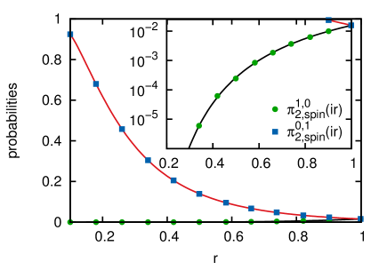
Figure 1: (color online) Ising spin clusters wrapping probability $\pi_{2,\mathrm{spin}}^{0,1}(ir)$ (blue squares and red line) and $\pi_{2,\mathrm{spin}}^{1,0}(ir)$ (green circles and black line) at $T_{c}$ vs. the aspect ratio $r$. The lines correspond to the expression of Eq. (13) and the symbols correspond to the results of simulations. The error bars are smaller than the symbols. In the inset the same probabilities are represented with the ordinate in logarithmic scale.

The agreement is excellent. Since in this range of aspect ratios $\pi_{2,\mathrm{spin}}^{1,0}(ir)$ is at most of order $10^{-2}$, hence barely visible, we add an inset with the ordinate in logarithmic scale. In Fig. 2, the probabilities for clusters winding once vertically and horizontally are presented. The sum $\pi_{2,\mathrm{spin}}^{1,1}(ir)+\pi_{2,\mathrm{spin}}^{1,-1}(ir)$ is shown instead of each one individually because of the symmetry relation $\pi_{2,\mathrm{spin}}^{1,1}(ir)=\pi_{2,\mathrm{spin}}^{1,-1}(ir)$. Even at its maximum at $r=1$ the sum is of the order of $5.10^{-5}$ which makes its numerical estimation less accurate than before but the agreement with the formula is still good. The probabilities for other homotopy groups are too small to allow a numerical estimation.

Figure 2: (color online) Ising spin clusters wrapping probability $\pi_{2,\mathrm{spin}}^{1,1}(ir)+\pi_{2,\mathrm{spin}}^{1,-1}(ir)$ (green circles and black line) at $T_{c}$ vs. the aspect ratio $r$. The line corresponds to the expression of Eq. (13) and the symbols correspond to the results of simulations.

5 Wrapping probabilities for cross clusters on untwisted tori

In this section we are interested in clusters contributing to the subgroup $\mathbb{Z}\times\mathbb{Z}$, i.e. cross-shaped clusters. In [37] Ziff et. al. obtained a closed form for cross clusters on untwisted tori ($\tau=ir$). They give a closed form only for percolation but it is possible to do the same for the FK and spin clusters as well. As seen in section 2, the partition function of interest $Z^{+}_{Q}$ is:

$$Z^{+}_{Q} = \frac{Q}{2}Z_{c}(g,1)=\frac{Q}{2}\sum_{m,m^{\prime}\in\mathbb{Z}}\left[Z_{m,m^{\prime}}(g)-Z_{m,m^{\prime}}(g/4)\right]$$ (14)

$$= \frac{Q}{2}\left[Z_{c}(4g,0)-Z_{c}(g,0)\right].$$

For untwisted tori ($\tau=ir$) $Z_{c}(g,0)$ becomes:

$$Z_{c}(g,0) = \sqrt{\frac{g}{r}}\frac{1}{|\eta(q)|^{2}}\sum_{m,m^{\prime}\in\mathbb{Z}}\exp\left[-\pi g\left(m^{2}r+\frac{m^{\prime 2}}{r}\right)\right]$$

$$= \sqrt{\frac{g}{r}}\frac{\theta_{3}\left(igr\right)\theta_{3}\left(\frac{ig}{r}\right)}{|\eta(q)|^{2}}$$

because in this case the sum over two integers reduces to a product of $\theta$ functions. Finally:

$$Z^{+}_{Q} = \frac{Q}{4}\sqrt{\frac{g}{r}}\frac{2\theta_{3}\left(igr\right)\theta_{3}\left(\frac{ig}{r}\right)-\theta_{3}\left(\frac{igr}{4}\right)\theta_{3}\left(\frac{ig}{4r}\right)}{|\eta(q)|^{2}}$$

This formula is valid for all $g$ but the probability is in general more complicated because of the total partition function. For the Ising model the probability is simply:

$$\pi^{+}_{Q}(r)=\frac{Q}{2|\eta(q)|}\sqrt{\frac{g}{r}}\frac{2\theta_{3}\left(igr\right)\theta_{3}\left(\frac{ig}{r}\right)-\theta_{3}\left(\frac{igr}{4}\right)\theta_{3}\left(\frac{ig}{4r}\right)}{|\theta_{2}\left(ir\right)|+|\theta_{3}\left(ir\right)|+|\theta_{4}\left(ir\right)|}.$$ (17)

Taking $g=3$ and $Q=2$ yields the result for the Ising FK clusters in agreement with the values obtained by Arguin. For spin clusters the probability is expected to be given by taking $g=16/3$ and $Q=1$. The situation is however slightly more subtle as a direct measurement from MC simulations shows that $\pi_{2,\mathrm{spin}}^{0}=0$ and that $\pi_{2,\mathrm{spin}}^{+}$ is twice the quantity given by Eq. (17). This can be explained by the fact that when spin clusters of a given color are all trivial then there exists a cluster of the other color wrapping in both direction and thus contributing to the subgroup $\mathbb{Z}\times\mathbb{Z}$. This means that no configuration can contribute to $\{0\}$ while considering simultaneously both colors. Furthermore one has to remember that we are extrapolating those results from the critical line using the mapping to a tricritical model with only one state. By doing so, one of the two spin values of the Ising spin is absorbed to generate the vacancies of the tricritical model. Hence considering one color at a time is natural when considering the properties of spin clusters. It makes no difference to the discussion for the configurations contributing to the subgroups $\{a,b\}$ since in this case at least one cluster of each color is present. However, for the cross-shaped clusters, it is necessary to consider only one color as those clusters come alone. This enables us to recover the relation $\pi_{2,\mathrm{spin}}^{0}=\pi_{2,\mathrm{spin}}^{+}$ expected with $Q^{\prime}=1$. Indeed, because of the symmetry between the two colors, considering only one color reduces the value $\pi_{2,\mathrm{spin}}^{+}$ measured in MC simulation by a factor two which is in agreement with Eq. (17) with $g=16/3$ and $Q=1$ .

Conclusion

In this work, we checked that the natural analytic continuation from the critical branch yields the correct results for the wrapping probabilities of Ising spin clusters. We also obtained an elegant expression for those wrapping probabilities. As a generalisation the study of the 3-Potts spin clusters is definitely interesting but might be more subtle as the mapping corresponds to a tricritical Potts model with a non integer number of states. This case is also interesting since the conjectured continuation to the tricritical branch is known to fail in some cases as already mentioned. This will be treated in another work.

References

- [1] C. M. Fortuin and P. W. Kasteleyn. On the random-cluster model : I. introduction and relation to other models. Physica, 57(4):536–564, February 1972.
- [2] A Coniglio and W Klein. Clusters and Ising critical droplets: a renormalisation group approach. J. Phys. A: Math. Gen., 13(8):2775, August 1980.
- [3] W. Janke and A. M. J. Schakel. Fractal structure of spin clusters and domain walls in the two-dimensional Ising model. Phys. Rev. E, 71(3):036703, March 2005.
- [4] A. L. Stella and C. Vanderzande. Scaling and fractal dimension of Ising clusters at the d=2 critical point. Phys. Rev. Lett., 62(10):1067, March 1989.
- [5] C. Vanderzande. Fractal dimensions of Potts clusters. J. Phys. A: Math. Gen., 25(2):L75, January 1992.
- [6] F. Y. Wu. The Potts model. Rev. Mod. Phys., 54(1):235, January 1982.
- [7] W. Janke and A. M. J. Schakel. Geometrical vs. Fortuin-Kasteleyn clusters in the two-dimensional q-state Potts model. Nucl. Phys. B, 700(1-3):385, November 2004.
- [8] Y. Deng, H. W. J. Blöte, and B. Nienhuis. Geometric properties of two-dimensional critical and tricritical Potts models. Phys. Rev. E, 69(2):026123, February 2004.
- [9] G. Delfino, M. Picco, R. Santachiara, and J. Viti. Spin clusters and conformal field theory. J. Stat. Mech., 2013(11):P11011, November 2013.
- [10] I. A. Kovács, E. M. Elçi, M. Weigel, and F. Iglói. Corner contribution to cluster numbers in the Potts model. arXiv:1311.4186 [cond-mat], November 2013.
- [11] D. Stauffer and A. Aharony. Introduction to percolation theory. Taylor & Francis, 1994.
- [12] J. L. Cardy. Critical percolation in finite geometries. J. Phys. A: Math. Gen., 25(4):L201–L206, February 1992.
- [13] R. P. Langlands, C. Pichet, P. Pouliot, and Y. Saint-Aubin. On the universality of crossing probabilities in two-dimensional percolation. J. Stat. Phys., 67(3):553–574, 1992.
- [14] H. T. Pinson. Critical percolation on the torus. J. Stat. Phys., 75(5-6):1167–1177, June 1994.
- [15] G. M. T. Watts. A crossing probability for critical percolation in two dimensions. J. Phys. A: Math. Gen., 29(14):L363, July 1996.
- [16] J. Cardy. Crossing formulae for critical percolation in an annulus. J. Phys. A: Math. Gen., 35(41):L565–L572, October 2002.
- [17] E. Lapalme and Y. Saint-Aubin. Crossing probabilities on same-spin clusters in the two-dimensional Ising model. J. Phys. A: Math. Gen., 34(9):1825–1835, March 2001.
- [18] L.-P. Arguin and Y. Saint-Aubin. Non-unitary observables in the 2d critical Ising model. Phys. Lett. B, 541(3-4):384–389, August 2002.
- [19] M. Bauer, D. Bernard, and K. Kytölä. Multiple Schramm-Loewner evolutions and statistical mechanics martingales. J. Stat. Phys., 120(5-6):1125–1163, September 2005.
- [20] M. J. Kozdron. Using the Schramm-Loewner evolution to explain certain non-local observables in the 2D critical Ising model. J. Phys. A: Math. Theor., 42(26):265003, July 2009.
- [21] O. Schramm. Scaling limits of loop-erased random walks and uniform spanning trees. Israel J. Math., 118(1):221–288, December 2000.
- [22] G. F. Lawler, O. Schramm, and W. Werner. On the scaling limit of planar self-avoiding walk. arXiv:math/0204277, April 2002.
- [23] S. Smirnov. Critical percolation in the plane: conformal invariance, Cardy’s formula, scaling limits. C.R.A.S. - Series I - Mathematics, 333(3):239–244, August 2001.
- [24] R. Langlands, P. Pouliot, and Y. Saint-Aubin. Conformal invariance in two-dimensional percolation. Bulletin of the American Mathematical Society, 30(1):1–61, 1994.
- [25] P. di Francesco, H. Saleur, and J. B. Zuber. Relations between the coulomb gas picture and conformal invariance of two-dimensional critical models. J. Stat. Phys., 49(1-2):57–79, October 1987.
- [26] L.-P. Arguin. Homology of Fortuin-Kasteleyn clusters of Potts models on the torus. J. Stat. Phys., 109(1):301–310, 2002.
- [27] A. Morin-Duchesne and Y. Saint-Aubin. Critical exponents for the homology of Fortuin-Kasteleyn clusters on a torus. Phys. Rev. E, 80(2):021130, 2009.
- [28] T. Blanchard and M. Picco. Frozen into stripes: Fate of the critical Ising model after a quench. Phys. Rev. E, 88(3):032131, September 2013.
- [29] K. Barros, P. L. Krapivsky, and S. Redner. Freezing into stripe states in two-dimensional ferromagnets and crossing probabilities in critical percolation. Phys. Rev. E, 80(4):040101, October 2009.
- [30] J. Olejarz, P. L. Krapivsky, and S. Redner. Fate of 2D kinetic ferromagnets and critical percolation crossing probabilities. Phys. Rev. Lett., 109(19):195702, November 2012.
- [31] T. Blanchard, L. F. Cugliandolo, and M. Picco. A morphological study of cluster dynamics between critical points. J. Stat. Mech., 2012(05):P05026, May 2012.
- [32] T. Blanchard, L. F. Cugliandolo, and M. Picco. How soon after a zero-temperature quench is the fate of the Ising model sealed? arXiv:1312.1712 [cond-mat], December 2013.
- [33] B. Nienhuis. Coulomb gas formulation of two dimensional phase transitions, volume 11 of Phase Transitions and Critical Phenomena, chapter 1, page 1. Academic Press London, 1987.
- [34] R. J. Baxter. Exactly Solved Models in Statistical Mechanics. Dover Publications, January 2008.
- [35] P. Di Francesco, P. Mathieu, and D. Senechal. Conformal Field Theory. Springer, 1997.
- [36] U. Wolff. Collective monte carlo updating for spin systems. Phys. Rev. Lett., 62(4):361, January 1989.
- [37] R. M. Ziff, C. D. Lorenz, and P. Kleban. Shape-dependent universality in percolation. Physica A, 266(1–4):17–26, April 1999.