Laser-induced magnetization curve

Abstract

We propose an all optical ultrafast method to highly magnetize general quantum magnets using a circularly polarized terahertz laser. The key idea is to utilize a circularly polarized laser and its chirping. Through this method, one can obtain magnetization curves of a broad class of quantum magnets as a function of time even without any static magnetic field. We numerically demonstrate the laser-induced magnetization process in realistic quantum spin models and find a condition for the realization. The onset of magnetization can be described by a many-body version of Landau-Zener mechanism. In a particular model, we show that a plateau state with topological properties can be realized dynamically.

I Introduction

Ultrafast control of magnetization has become a hot topic recently Kimel05 ; Kampfrath11 ; Kirilyuk10 ; Vicario13 ; Miyashita95 ; Miyashita98 ; Thomas96 . Not only does this technique have much potential for application, e.g., fast data storage and spintronics Zutic04 , but it also poses an important question in fundamental physics: Can we coherently induce an ultrafast phase transition in many-body quantum systems? Terahertz (THz) laser Fulop11 ; Hoffmann09 ; Hirori11 ; Matsunaga13 ; SatoGonokami13 is preferred in terms of quantum coherence since its photon energy is comparable with the energy scale of spin systems. Among spin systems, quantum antiferromagnets are known to show rich many-body effects. A traditional way to study their properties is to measure the magnetization curve, i.e., relation between magnetization and externally applied magnetic field. Prominent phenomena such as various magnetization plateaux Oshikawa97a ; Takigawa11 , field induced topological states Tanaka09 ; Oshikawa00 , and Bose-Einstein condensation of magnons Nikuni00 ; Giamarchi08 have been discovered. However, the magnetization curve up to the saturated magnetization often requires an extremely high magnetic field. If we can realize the full magnetization process in table-top laser experiments, studies on nontrivial magnetic phenomena would be more accessible, but it is not easy due to the limited laser strength. The magnetic field component of a THz laser is typically less than 0.5 T, several orders below the necessary field strength ($\sim 10-100$ T and more) for full magnetization.

We can overcome this difficulty with help from recent progress of quantum many-body systems in time-periodic external fields, which have been studied both theoretically Oka09 ; Kitagawa11 ; Lindner11 ; Takayoshi13 ; Sato14 and experimentally Wang13 . In general quantum magnets, a proper unitary transformation maps a rotating magnetic field of a circularly polarized laser into an effective static magnetic field Takayoshi13 ; Ruckriegel12 . If the magnetic field rotates in the $xy$ plane, the effective static field has a component in the $z$ direction, and its strength is given by the photon energy $\Omega$. For example, a laser with frequency of 1 THz ($\Omega=$1 THz$\sim 4$ meV) can typically produce an effective field as strong as $40$ T. Even stronger fields are obtained by increasing frequency $\Omega$, and it is reasonable to consider a possibility of “laser-induced magnetization curves”.

Our proposal is to change $\Omega$ from a small value to a larger value as slowly as possible. In other words, an upchirped THz laser pulse is required SatoGonokami13 ; Kamada13 . In this paper, starting from the zero field ground state (GS), we show that the system under a upchirped laser almost follows the GS in static magnetic field up to full magnetization in time evolution of the wave function. This is a significant difference compared with an equilibrium magnetization curve obtained using high magnetic field facilities since we can wait for a sufficiently long time in order to make the system equilibrated in the latter case. Thus, we need to find an appropriate protocol to realize the laser-induced magnetization curve. We determine ideal conditions to approach highly magnetized states and explain the mechanism by many-body Landau-Zener (LZ) tunnelings Landau32 ; Zener34 . In addition, in a particular model, we show that a symmetry protected topological (SPT) plateau state Pollmann10 ; Gu09 can be realized in this manner.

This paper is organized as follows. In Sec. II, we explain our idea about realizing laser-induced magnetization processes. Following the idea of Sec. II, we numerically demonstrate that a laser-induced magnetization indeed occurs in two simple but realistic quantum spin systems in Sec. III. It is also shown that a magnetization plateau state having topological properties is reproduced by circularly polarized laser. Sections IV and V are devoted to the quantitative discussion about the laser-induced magnetization curves obtained in Sec. III. We consider time evolution of wave functions from the viewpoint of the LZ tunneling mechanism in Sec. IV. We also obtain the “phase diagram” for the laser-induced plateau state of Sec. III, which leads to an ideal condition for the realization of laser-induced magnetization curves. In Sec. V, we investigate how close the dynamically laser-induced plateau state in Sec. III is to the equilibrium plateau state. Finally we summarize and discuss our results in Sec. VI.

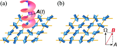
Figure 1: (Color online) (a) Quantum magnet in a circularly polarized laser. (b) Effective static system after the unitary transform (2).

II Basic Idea

In this section, we explain our basic idea for realization of laser-induced magnetization process. We consider general quantum magnets under a circularly polarized laser as shown in Fig. 1(a). The magnetic field of the laser generates a dynamical Zeeman interaction, which results in a Hamiltonian,

$${\cal H}(t)={\cal H}_{0}-A_{x}(t)S^{x}_{\rm tot}-A_{y}(t)S^{y}_{\rm tot}.$$ (1)

The first term ${\cal H}_{0}$ is the spin Hamiltonian and the magnetic field of the laser $(A_{x},A_{y})=A(\cos(\Omega t),\sin(\Omega t))$ rotates in the $xy$ plane. The operator $S_{\rm tot}^{\alpha}$ is the $\alpha$ component of the total spin and $\Omega$ is the laser frequency. Here we assume that the spin Hamiltonian ${\cal H}_{0}$ is invariant under U(1) spin rotation around the $S^{z}$ axis. If we apply the time-dependent unitary transform

$$U=\exp({\rm i}\Omega S_{\rm tot}^{z}t)$$ (2)

to such U(1)-symmetric magnets under the laser, we obtain the following relation,

$$U({\cal H}(t)-i\partial_{t})U^{-1}={\cal H}_{0}-\Omega S_{\rm tot}^{z}-AS_{\rm tot}^{x}-i\partial_{t}.$$

This transform maps the system from the experimental frame to a rotating frame in spin space Takayoshi13 ; Ruckriegel12 . In this rotating frame, the Hamiltonian becomes static as follows (see Fig. 1(b)):

$${\cal H}_{\rm eff}={\cal H}_{0}-B_{z}S^{z}_{\rm tot}-B_{x}S^{x}_{\rm tot}\quad(B_{z}=\Omega,\;B_{x}=A).$$ (3)

We emphasize that this mapping from the dynamical system (1) to the static one (3) always holds when the laser is circularly polarized and ${\cal H}_{0}$ is U(1) symmetric around the $S^{z}$ axis. The mapping does not depend at all on spatial dimensions, spin magnitude $S$, and the other details.

Equation (3) indicates that a laser with high frequency $\Omega$ can lead to highly magnetized states due to the effective Zeeman term $-\Omega S_{\rm tot}^{z}$. It also implies that the magnetization points in the opposite direction by changing the helicity of the laser. As we mentioned in the Sec. I, it is difficult to increase the magnitude $A$ to a large value, while the laser frequency $\Omega$ can be relatively easily tuned SatoGonokami13 . Therefore, the magnetization along the $S^{z}$ axis, $\langle S_{\rm tot}^{z}\rangle$, is expected to grow by increasing $\Omega$.

However, we should note that even if we increase $\Omega$, the wave function of the magnet does not always follow the GS of the effective static Hamiltonian (3). Instead, the system may be in the excited states and the magnetization may be small or even absent. In fact, when ${\cal H}_{0}$ has SU(2) spin-rotational symmetry, one can understand that the growth of the magnetization does not occur as follows. The effective Hamiltonian ${\cal H}_{\rm eff}$ represents a quantum magnet under a static magnetic field $\boldsymbol{B}=(A,0,\Omega)$. In the SU(2)-symmetric case, ${\cal H}_{0}$ and the Zeeman term $-\boldsymbol{B}\cdot\boldsymbol{S}_{\rm tot}$ commute with each other. As a result, the total spin exhibits just a simple precession motion around the $\boldsymbol{B}$ axis. This clearly indicates the absence of static growth of total magnetization. From this argument, we find that a magnetic anisotropy breaking the U(1) symmetry around the $\boldsymbol{B}$ axis is necessary to generate nonzero static magnetization. Notice that if the magnetic anisotropy conserves the U(1) symmetry about the $S^{z}$ axis, the mapping to the static system (3) is still valid. Fortunately, magnetic anisotropy generally exists in real magnetic materials.

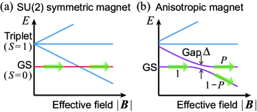
Figure 2: (Color online) (a) Low-energy excitations as a function of the effective field $|\boldsymbol{B}|$ in a SU(2)-symmetric magnet ${\cal H}_{0}$ and (b) in a magnet with magnetic anisotropy.

Based on a simple symmetry argument, let us qualitatively compare time evolution of quantum states in anisotropic and isotropic (SU(2)-symmetric) magnets, increasing the frequency $\Omega$. We assume that the GS of the SU(2)-symmetric magnet is paramagnetic with $S=0$. Usually, its lowest excitation is given by spin-$1$ triplet with $S=1$. If $\Omega$ (i.e., the effective field $|\boldsymbol{B}|$) is increased, the triplet excitations are split due to the Zeeman effect as shown in Fig. 2(a). At a certain value of $\Omega$, a level crossing occurs between the GS and the lowest excitation of the triplet. However, if we start from the GS, the wave function is still equivalent to the GS even after the level crossing since there is no matrix element between the lowest two states due to the SU(2) symmetry. On the other hand, if we consider a magnet with magnetic anisotropy, the level crossing generally changes into an avoided crossing as shown in Fig. 2(b). When the frequency $\Omega$ is monotonically increased, some weight of the wave function continuously follows the lowest-energy state and the total magnetization grows by unity, while the remaining weight tunnels into the upper state. This phenomenon would be described by the LZ tunneling picture Landau32 ; Zener34 . With further increasing of $\Omega$, avoided crossings between the lowest two states successively take place and the magnetization would gradually grow. In order to make a larger weight of the state follow the GS of Eq. (3), we have to suppress the LZ tunneling probability $P$ in Fig. 2(b). From a theory of two-level LZ tunneling, the probability $P$ is known to rapidly decrease with decreasing the varying speed of $\Omega$. This argument based on the LZ tunneling clearly indicates that we should raise $\Omega$ as slowly as possible to realize magnetized states by the laser. Namely, an adiabatic change of $\Omega$ is ideal. Thanks to the recent development of laser technique, we can prepare lasers with gradually increasing its frequency $\Omega$. This technique is called chirping SatoGonokami13 ; Kamada13 .

In conclusion, the argument in this section tells us that circular polarization, magnetic anisotropy, and chirping of laser would be significant for the realization of laser-induced magnetization process. Even if the magnetic anisotropy slightly breaks the U(1) symmetry, laser-induced magnetization is expected to occur.

III Laser-induced Magnetization Process

The idea of the laser-induced magnetization process discussed in the previous section could be applied to general quantum magnets. In the remaining part of this paper, in order to quantitatively study the laser-induced dynamics, we concentrate on two simple but realistic one-dimensional (1D) spin-1/2 systems: Heisenberg antiferromagnetic (HAF) and ferro-ferro-antiferromagnetic (FFAF) models. The HAF model explains properties of many quasi-1D magnetic materials while the FFAF model exhibits a 1/3 magnetization plateau state with a SPT order as explained below, which describes $\rm Cu_{3}(P_{2}O_{6}OH)_{2}$ Hase06 ; Hase07 ; Hida94 . The spin Hamiltonians are respectively given by

$${\cal H}_{\rm HAF}= \sum_{j=1}^{L}J\boldsymbol{S}_{j}\cdot\boldsymbol{S}_{j+1},$$

$${\cal H}_{\rm FFAF}= \sum_{j=1}^{L/3}(-J_{\rm F}\boldsymbol{S}_{3j-2}\cdot\boldsymbol{S}_{3j-1}-J_{\rm F}\boldsymbol{S}_{3j-1}\cdot\boldsymbol{S}_{3j}$$

$$\qquad+J_{\rm AF}\boldsymbol{S}_{3j}\cdot\boldsymbol{S}_{3j+1}),$$

where $\boldsymbol{S}_{j}$ is the spin-1/2 operator on site $j$ and $L$ is the system size. Coupling constants $J$, $J_{\rm F}$, and $J_{\rm AF}$ are all positive.

If ${\cal H}_{0}$ is SU(2) symmetric, ${\cal H}_{0}$ commute with $S_{\rm tot}^{x,y,z}$. In this case, magnetic (static) and laser (dynamic) parts in the time evolution operator are separated ($e^{-i{\cal H}(t)t}=e^{-i{\cal H}_{0}t}e^{i(A_{x}(t)S^{x}_{\rm tot}+A_{y}(t)S^{y}_{\rm tot})t}$), and the magnetization dynamics becomes trivial. As we mentioned in Sec. II, we have to include a term that breaks SU(2) symmetry in ${\cal H}_{0}$ to lead to nonzero magnetization. As a small magnetic anisotropy term in ${\cal H}_{0}$, we here introduce a staggered Dzyaloshinsky-Moriya (DM) interaction Dzyaloshinsky58 :

$${\cal H}_{\rm DM}=\sum_{j=1}^{L}(-1)^{j}\boldsymbol{D}\cdot\boldsymbol{S}_{j}\times\boldsymbol{S}_{j+1}$$

with a DM vector $\boldsymbol{D}=(0,0,D)$ ($D\ll J,J_{\rm AF},J_{\rm F}$). Such an anisotropy often appears in quasi-1D magnets Dender97 ; Asano00 ; Feyerherm00 ; Kohgi01 ; Oshikawa97b ; Sato04 . Note that any types of magnetic anisotropy such as Ising and single-ion anisotropies play the same role.

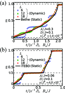
Figure 3: (Color online) Laser-induced magnetization curves of (a) the HAF model and (b) the FFAF model with $J_{\rm F}=J_{\rm AF}=J$ realized by an upchirped circularly polarized laser in the slow chirp limit. Solid lines are static magnetization curves from (3) obtained by Bethe ansatz and iTEBD ($D=B_{x}=0$). The horizontal axes for the dynamical and static process are $t/(v^{-1}J)(=\Omega(t)/J)$ and $B_{z}/J$, respectively.

We numerically study real time evolution of the wave functions in two models ${\cal H}_{\rm HAF}$ and ${\cal H}_{\rm FFAF}$ with a staggered DM term under a circularly polarized laser. We start from the GS of ${\cal H}_{0}$, and then apply an upchirped circularly polarized laser. The pulse laser is modeled as follows. (i) Switch on: We first increase the amplitude from 0 to $A$ during $t=-10^{3}J^{-1}$ to 0. During this process, $\Omega$ is zero. (ii) Chirping: We linearly increase the frequency as

$$\Omega(t)=vt,$$

where $v$ is the chirping speed, i.e., the magnetic field of applied laser is represented as $(A_{x},A_{y})=A(\cos(vt^{2}/2),\sin(vt^{2}/2))$. In order to mimic an experimental situation, we consider the case where the maximum field strength $A$ is small enough, e.g., $A/J,A/J_{\rm F,AF}\ll 1$, while $\Omega$ can increase up to a large value such as $\Omega/J,\Omega/J_{\rm F,AF}\sim 1$. Though the increase of $A$ and $\Omega$ occurs simultaneously in real laser pulses, here we split them into two processes to understand the effect of chirping alone.

We first calculate the GSs of ${\cal H}_{\rm HAF}+{\cal H}_{\rm DM}$ and ${\cal H}_{\rm FFAF}+{\cal H}_{\rm DM}$ by exact diagonalization in finite systems ($L=6,12,18$), and then numerically integrate the time-dependent Schrödinger equation $i\frac{d}{dt}|\Psi(t)\rangle={\cal H}(t)|\Psi(t)\rangle$ for the magnets under a circularly polarized laser, using the fifth order Runge-Kutta method. Hereafter, we use the normalized magnetization:

$$m\equiv M_{\rm tot}/M_{\rm tot}^{\rm st},$$

where $M_{\rm tot}\equiv\langle S_{\rm tot}^{z}\rangle$ and $M_{\rm tot}^{\rm st}$ is its saturated value.

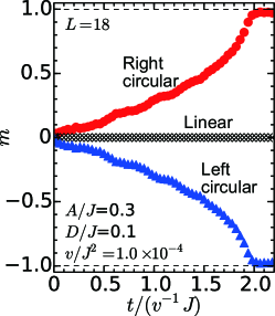
Figure 4: (Color online) Laser-induced magnetization curves of the 1D HAF model with $L=18$ in right-circularly, left-circularly, and linearly polarized lasers. We have used the same parameters as those of Fig. 3(a).

Figure 3(a) shows the laser-induced magnetization curve of the HAF model plotted against the time. The chirping speed $v$ is set to a very small value. We will study the $v$ dependence later. The curve is compared with the equilibrium one of the effective Hamiltonian (3) in static field $B_{z}$ with $B_{x}=D=0$ obtained by Bethe ansatz Qin97 ; Cabra98 . Here we have ignored $B_{x}$ and $D$ in the static calculation since they are very small. We observe that the laser-induced magnetization curve converges to the static curve in the large $L$ limit. The FFAF model shows similar behaviors with one additional feature: the $m=1/3$ plateau state. As plotted in Fig. 3(b), with increasing $L$, the laser-induced magnetization curve also converges to the static curve obtained by infinite time evolving block decimation (iTEBD) Vidal07 with matrix dimension $\chi=150$. During the process, the magnetization shows a plateau around $m=1/3$ with a width almost independent of the system size. We also confirmed the realization of 1/3 plateau for the same models with other anisotropies such as Ising-type and uniform DM interaction.

In addition to the FFAF model, we also numerically confirmed that a laser-induced dynamical 1/3 plateau can be observed in a 1D $J_{1}$-$J_{2}$ spin model Maeshima03 ; Okunishi03 ; Okunishi08 ; Hikihara10 . However, this system requires stronger DM interaction with $D\sim{\cal O}(J_{1,2})$ for generating the laser-driven plateau. This would be because the transition to the plateau phase is accompanied with a spontaneous breakdown of translational symmetry in the $J_{1}$-$J_{2}$ model (any symmetry breaking does not take place in the plateau of the FFAF model). A plateau with a broken symmetry is more fragile against perturbation than that with no symmetry breaking.

As we mentioned in Sec. II, if we change the sign of laser frequency from $\Omega$ to $-\Omega$, which is equivalent to changing the polarization of the laser, the magnetization is expected to point in the opposite direction. We confirm this prediction in the one-dimensional (1D) HAF model. Figure 4 shows numerical results for laser-induced magnetization curves of the HAF chain under right-circularly, left-circularly, and linearly polarized lasers with small chirping speed $v$. As expected, the magnetizations for right- and left-circularly polarized lasers are antiparallel with each other and linear polarization does not induce magnetization. In fact, we can prove rigorously that the size of induced magnetization is the same and the direction is opposite for right- and left-circularly polarized lasers applied to HAF and FFAF magnets with Ising, uniform DM, and staggered DM anisotropies (see Appendix A). It is also shown that the magnetization induced by linearly polarized laser is exactly zero. Although such a rigorous proof does not exist in general systems (e.g., systems in more than one dimension), it is expected that the magnetization points in the opposite direction if circular polarization is reversed. Moreover, a linearly polarized laser would not be useful for the magnetization growth.

IV Landau-Zener tunneling

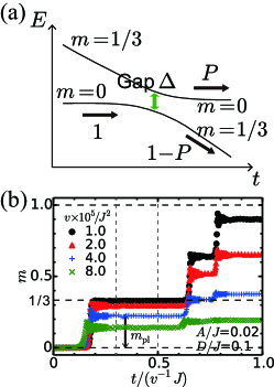
Figure 5: (Color online) (a) Schematic picture of the LZ tunneling. (b) Laser-induced magnetization curves of the $L=6$ 1D FFAF model for different chirping speed $v$. The height $m_{\rm pl}$ of the 1/3 plateau is defined as the average within $0.3\leq t/(v^{-1}J)\leq 0.5$ (vertical dashed lines).

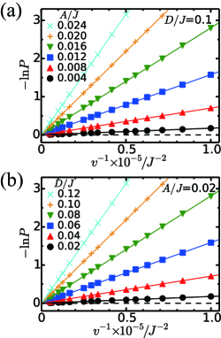
Figure 6: (Color online) Plots of $-\ln P$ as a function of $v^{-1}$ (a) varying $A$ with fixed $D$ and (b) varying $D$ with fixed $A$. Solid lines show fittings of the data with a function $-\ln P\propto v^{-1}$.

As shown in the previous section, if the chirping speed $v$ is sufficiently slow, it is possible to realize fully polarized magnetization as well as magnetization plateau states. Then, the natural question is “How slow should it be to see the plateau?” It is crucial in finite width pulses.

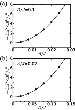
Figure 7: (Color online) Scaling $-v\ln P$ ($\propto\Delta^{2}$) (a) as to $A$ with fixed $D$ and (b) as to $D$ with fixed $A$. Solid lines represent fittings with a function (a) $-v\ln P\propto A^{2}$ and (b)$-v\ln P\propto D^{2}$.

To answer the question, we study the $v$ dependence of the magnetization curve. Figure 5(b) shows that of the FFAF chain with $J_{\rm F}=J_{\rm AF}=J$ and $L=6$. We notice that the height of the $1/3$ plateau becomes lower as the speed becomes faster (note that other plateau-like states in Fig. 5(b) are attributed to finite-size effect). This reduction can be explained by the LZ tunneling picture Miyashita95 . When $v$ is sufficiently small, we can understand the magnetization dynamics from the effective static model (3). As we increase $\Omega(=B_{z})$, the excited state with magnetization $m=1/3$ lowers its energy due to the Zeeman term $-\boldsymbol{B}\cdot\boldsymbol{S}_{\rm tot}$ and crosses the GS ($m=0$ sector) at a certain value of $\Omega$. (Strictly speaking, $S_{\rm tot}^{z}$, i.e., $m$, is not a good quantum number due to the presence of transverse field $A(=B_{x})$ term. However, we assume that $B_{x}$ is much smaller than $B_{z}=\Omega$ and $S_{\rm tot}^{z}$ can be approximated as a conserved quantity.) Since $A$ and $D$ are finite and the spin-rotational symmetry is broken, the crossing becomes an avoided crossing, where we denote the gap between the $m=0$ and $m=1/3$ sectors as $\Delta$ (Fig. 5(a)). In the present case of the $L=6$ FFAF model, this avoided crossing takes place at $t/(v^{-1}J)=\Omega/J\sim 0.174$. The wave function $|\Psi(t)\rangle$ is initially given by the GS ($m=0$). After the LZ tunneling around the avoided crossing point, $|\Psi(t)\rangle$ becomes a linear superposition of the $m=1/3$ state (new GS) and the $m=0$ state (new excited state). Let us represent the probability of being in the new excited state and GS by $P$ and $1-P$, respectively. We can relate $P$ with the plateau height. To make this concrete, we define the averaged height $m_{\rm pl}$ as a mean value of $m$ within $0.3\leq\Omega/J\leq 0.5$ (Fig. 5(b)). For the $1/3$ plateau, we can extract a relation $m_{\rm pl}=(1-P)/3$. Then we can estimate $P$ from the numerically determined $m_{\rm pl}$. The LZ formula for the tunneling probability $P$ in a two-level system is known to be Landau32 ; Zener34

$$P=\exp(-c\Delta^{2}/v),$$ (4)

with a constant $c$. In order to verify whether this formula holds in our many-body problem, we numerically calculate $m_{\rm pl}$ for various values of $A$, $D$, and $v$. We plot $-\ln P$ as a function of $v^{-1}$ in Fig. 6. The data for fixed $A$ and $D$ are well fitted with a linear function (solid lines), which indicates the validity of Eq. (4). Figure 7 shows that $-v\ln P$ is well fitted with $\propto A^{2}$ ($\propto D^{2}$) for fixed $D$ (A). Therefore, from the relation $-v\ln P=c\Delta^{2}$, the dependence of the tunneling gap on $A$ and $D$ is

$$\Delta\propto AD.$$ (5)

At first glance, it may appear unexpected that the gap depends not only on the material parameter $D$ but also on the external field strength $A$. The most intuitive reasoning is that we need both anisotropy and rotating magnetic field to induce a finite magnetization. Then Eq. (5) is just the leading order in the series expansion. We can arrive at the same conclusion more systematically using a perturbation theory with respect to $D$ and $A$ (see Appendix B for details of the calculation).

In Fig. 8, we show a “phase diagram” for realizing the plateau state in the parameter space of field strength $A$ and chirping speed $v$ for the 1D FFAF model with $J_{\rm F}=J_{\rm AF}=J$ and $L=12$. We represent contours of plateau height $m_{\rm pl}=0.3$ and 0.1 by dashed and dotted lines, respectively. The phase diagram clearly indicates that strong laser with slow chirping speed (the bottom right part in Fig. 8) is preferred for achieving a magnetization plateau with large magnetization. We define a “nearly 1/3 plateau” region as $m_{\rm pl}>0.3$ (lower than the dashed line, colored with shade). This region has a domelike structure with a peak near $A/J\sim 0.04$. On the left side of the peak ($A/J<0.04$), the boundary is parabolic in $A$, which can be understood by the LZ tunneling. Using Eqs. (4) and (5), the criterion for a sharp laser-induced plateau is ($\alpha$: nonuniversal constant)

$$v/A^{2}<\alpha D^{2},$$ (6)

which explains the parabolic feature of the contour $m_{\rm pl}=0.3$. To make connection with experiment, we note that if we assume $J=10$ meV, $A=0.4$ meV $\sim 4$ T, and $D=1$ meV, then $v\sim 10^{-4}J^{2}\sim 6\times 10^{-4}$ THz/ps is necessary for Eq. (6). We also mention that other magnetic anisotropies will play the same role as the DM interaction $D$ in Eq. (6).

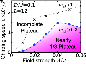
Figure 8: (Color online) “Phase diagram” of the laser-driven 1/3 plateau state of the FFAF model with $J_{\rm F}=J_{\rm AF}=J$ in the parameter space $(A,v)$. The dashed and dotted lines are contours of plateau height $m_{\rm pl}=0.3$ and 0.1, respectively. This tells us the condition for realizing an ideal plateau state with large magnetization.

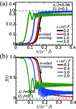
Figure 9: (Color online) Time evolution of (a) magnetization $m$ and (b) overlap $f(t)$ between a wave function at time $t$ and the initial state for various chirping speed $v$. Arrows represent the time when the system goes through an avoided crossing ($t/(v^{-1}J)\sim 0.174$).

In the strong field side ($A/J>0.04$), the contour $m_{\rm pl}=0.3$ starts to bend down. It implies that this region cannot be understood by the LZ formula. To see how the LZ theory breaks down, we perform numerical simulations at $A/J=0.06$ for various chirping speeds $v$. In addition to the magnetization $m$, we calculate the overlap $f(t)$ between the wave function $|\Psi(t)\rangle$ at time $t$ and the initial state $|\Psi(0)\rangle$:

$$f(t)\equiv|\langle\Psi(0)|\Psi(t)\rangle|^{2}.$$

The results are presented in Fig. 9. For small $v$, the increase of $m$ and the drop of $f(t)$ happens around $t/(v^{-1}J)\sim 0.174$, indicated by arrows in Fig. 9. The corresponding frequency $\Omega/J\sim 0.174$ is almost equal to the point of the minimum gap in Fig. 5(a). Therefore, for small $v$, the LZ tunneling picture is valid and the transition from the initial state ($m=0$) to the plateau state ($m=1/3$) instantly happens around the single point $t/(v^{-1}J)\sim 0.174$. However, when the chirping speed becomes fast, i.e., larger $v$, this picture starts to fail. The increase of $m$ and drop of $f(t)$ start earlier than $t/(v^{-1}J)\sim 0.174$, and both quantities show oscillations. The LZ theory assumes that the tunneling happens at a single point where the energy gap is smallest, that is, the avoided crossing point (see Fig. 5(a)). In the region of $A/J>0.04$, this necessary condition for the LZ theory is violated. It is presumably because a direct hybridization between the initial ($m=0$) and plateau ($m=1/3$) states begins before the LZ tunneling takes place due to the strong laser amplitude $A/J$. An oscillation seen in $m$ and $f(t)$, supposedly caused by a difference of phase factor between the initial and plateau states, supports our speculation. In addition, a hybridization is concerned with not only these two states but also other states with higher energy, which makes the LZ picture even worse. In the result, a crossover from the LZ mechanism in the weak field side ($A/J<0.04$) to a direct hybridization in the strong field side ($A/J>0.04$) leads to the domelike structure.

V Plateau with SPT order

Finally, we discuss topological properties of the dynamically induced $1/3$ plateau state in the 1D FFAF model. First, we study the GS of the FFAF model in static field $B_{z}$ using iTEBD. The SPT order in spin systems can be detected by the entanglement spectrum (ES) Pollmann10 ; Gu09 . To define ES for a quantum state $|\psi\rangle$, we divide the system into two subspaces A and B. From the Schmidt decomposition $|\psi\rangle=\sum_{i}\lambda_{i}|\psi_{\rm A}\rangle_{i}\otimes|\psi_{\rm B}\rangle_{i}$, the ES is defined as $-\ln(\lambda_{i}^{2})$ $(i=1,\ldots,\chi)$, where $\lambda_{i}$ is normalized as $\sum_{i}\lambda_{i}^{2}=1$. In the FFAF model, we evaluate the ES by cutting the system at the antiferromagnetic bond $J_{\rm AF}$, and the result is plotted in Fig. 10(b). We see that the ES is doubly degenerate in the plateau state at $B_{z}/J=0.4$, but there is no degeneracy at $B_{z}/J=0.1$ and 0.7. This degeneracy is a clear signature of the SPT order in the $1/3$ plateau state. In fact, we can relate this state with a valence bond solid (VBS) state Affleck87 as follows. As schematically shown in Fig. 10(a), in the limit of $J_{\rm F}\gg J_{\rm AF}$, ferromagnetically coupled three adjacent $S=1/2$ spins can be regarded a “site” with $S=3/2$, and neighboring trimers are coupled by an antiferomagnetic bond $J_{\rm AF}$. In the 1/3 plateau state, one of the three spin-1/2 components is fully polarized (represented by an arrow), and the remaining two spins form singlet pairs (solid line) with their neighbors. If we assume that this VBS picture of the plateau state survives up to $J_{\rm F}\sim J_{\rm AF}$, the plateau must possess the same topological nature as the Haldane state in the $S=1$ HAF model Affleck87 ; Haldane83 . This argument clearly explains the double degeneracy of the ES in the plateau state. The symmetry protection of magnetization plateau states will be discussed in detail elsewhere TakayoshiTBA .

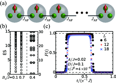
Figure 10: (Color online) (a) Schematic VBS picture of the static 1/3 plateau phase in the FFAF chain. (b) ES of the static magnetized states in the FFAF chain with $D=0$ calculated by iTEBD ($\chi=150$). The system is partitioned at an antiferromagnetic bond. (c) Fidelity of the laser-induced dynamical state with respect to the static plateau with the SPT order.

We next turn to the laser-induced plateau state. How close is the dynamical plateau state to the static SPT state? To answer this question, we calculate the fidelity (overlap):

$$F(t)\equiv\big{|}\langle\Phi_{\rm topo}^{\rm st}|\Psi(t)\rangle\big{|}^{2}$$

by numerical diagonalization, where $|\Phi_{\rm topo}^{\rm st}\rangle$ represents the static GS of the FFAF chain in $B_{z}/J=0.4$ ($D=A=0$) and $|\Psi(t)\rangle$ is the laser-induced state. Figure 10(c) shows that the overlap $F(t)$ is larger than 95 % when the dynamical state $|\Psi(t)\rangle$ is in the plateau phase ($0.2\lesssim B_{z}/J\lesssim 0.6$) while $F(t)\sim 0$ when $|\Psi(t)\rangle$ is outside the plateau phase. This result is almost independent of the system size $L$. Thus, we conclude that if the chirping speed $v$ is sufficiently small, the SPT phase can be achieved dynamically. In a rigorous sense, we have to switch off the laser amplitude or neglect the DM anisotropy in order to protect the topological properties of the dynamical plateau state Pollmann10 . Such a subtlety can be avoided in the case of Ising anisotropy.

VI Conclusion and Discussions

We have proposed a novel scheme of “laser-induced magnetization curves” for general quantum magnets. An upchirped circularly polarized laser in the THz regime is required, and the material must have small but finite magnetic anisotropy. From our numerical calculation in realistic spin models, the criterion for laser strength and chirping speed was obtained, which is explained by the LZ picture. Using this method, it is even possible to realize a SPT phase dynamically. In this paper, we have demonstrated laser-induced magnetization curves in two types of magnets: HAF and FFAF chains. However, as can be seen from our analyses, this phenomenon does not exploit specific properties of these magnets. Therefore, we again stress that laser-induced magnetization curves would be attained by laser chirping in a wide variety of magnetic materials in any dimension. We also note that the direction of the magnetization growth can be changed by switching the helicity of the laser.

In addition to the above necessary condition for the magnetization dynamics, let us briefly discuss some desired conditions for easily realizing a higher value of laser-induced magnetization. Large magnetic anisotropies are desired to open a wide gap $\Delta$ in Fig. 5(a). Magnets with large spin magnitude $S$ are preferred since the value $S$ is regarded as the coupling constant of the Zeeman term, namely a large value $S$ helps the laser amplitude to effectively increase. When the Zeeman coupling is too small, effects of the laser might be masked by several noises such as thermal fluctuation, dipole interaction, spin-phonon coupling, and so on. Magnets with ferromagnetic exchanges are also favorable since a ferromagnetic interaction generally decreases the value of saturation field and it reduces the necessary time of chirping. The time interval of chirping needed for full magnetization curves in Fig. 3 is estimated to be about $2.0\times 10^{4}J^{-1}$ for both HAF and FFAF chains. Assuming $J\sim 10$ meV ($J^{-1}\sim 0.4$ ps), it amounts to $2.0\times 10^{4}J^{-1}\sim 8$ ns. It is generally difficult to generate an ideal upchirped laser for a long time interval in real experiments. However, even a nonideal laser is expected to generate a finite magnetization if the laser frequency is comparable to the exchange coupling of the target materials Takayoshi13 . In an actual experimental setup, heating caused by laser would smear the plateau structure. In order to prevent such heating, we should choose the laser frequency far from any resonant frequencies of phonons, magnons, etc.: excitations which thermalize the sample. Furthermore, if the LZ gap is large enough (thanks to, e.g., large Zeeman coupling), a laser would induce a finite magnetization before the temperature considerably increases.

A pump-probe experiment with two laser pulses would be one of the simple realistic ways of measuring laser-induced magnetizations. We prepare a circularly polarized laser pulse to coherently control the magnetization of a target material. The other pulse is used to measure the magnetization, for example, through the inverse Faraday or Kerr effect. Notice that the laser-induced magnetization curve differs considerably from standard magnetic resonance phenomena. Our scheme does not have a specific energy scale concerning the laser frequency $\Omega$ (although $\Omega$ should be the order of exchange couplings) while a magnetic resonance usually happens (or becomes strong) at a certain frequency characteristic of the magnet.

Effects of dissipation from an environment and heating magnets by laser, which are not considered here, are important future problems. In this paper, to see the laser-driven dynamics of magnets, we have focused on finite-size systems. Investigation on the effects of laser in the thermodynamic limit is another important issue.

We finally comment on a possible combination of the current method and actual static magnetic fields. Namely, a static Zeeman term $B_{\rm st}S_{\rm tot}^{z}$ can be added to ${\cal H}_{0}$, and after the mapping from Eq. (1) to Eq. (3), the total effective field becomes

$$B^{\rm total}_{z}=\Omega+B_{\rm st}.$$ (7)

This fact would be practically useful in experiments. For example, we can study the destruction and recovery of the topological state starting from the plateau state in finite static fields and then applying a pulse circularly polarized laser.

Appendix A Relation between laser polarization and induced magnetization

Magnetization $m(>0)$ along the $z$ axis is induced when a right-circularly polarized laser $A(\cos(\Omega t),\sin(\Omega t))$ is applied to HAF and FFAF magnets with anisotropy. In the following, we prove that the induced magnetization becomes $-m$ for an application of a left-circularly polarized laser $A(\cos(\Omega t),-\sin(\Omega t))$ in the case of HAF and FFAF magnets with anisotropies of (i) Ising, (ii) uniform DM, and (iii) staggered DM types. In addition, we can show that magnetization along the $z$ axis is exactly zero ($m=0$) for a linearly polarized laser $A(\cos(\Omega t),0)$. We write the time-dependent Schrödinger equation for the right-circularly (left-circularly) polarized laser as

$$i\partial_{t}|\Psi_{\rm R(L)}(t)\rangle={\cal H}_{\rm R(L)}|\Psi_{\rm R(L)}(t)\rangle.$$

The initial states are the same, $|\Psi_{\rm R}(0)\rangle=|\Psi_{\rm L}(0)\rangle$.

(i) Ising anisotropy: Let us consider $\pi$ rotation around the $x$ axis, $\pi_{x}$. This rotation $\pi_{x}$ changes $S_{\rm tot}^{z}$ to $-S_{\rm tot}^{z}$ and reverses the circular polarization from right to left in the Zeeman term. On the other hand, it keeps ${\cal H}_{\rm HAF}$, ${\cal H}_{\rm FFAF}$, and Ising anisotropy $J_{z}\sum_{j=1}^{L}S_{j}^{z}S_{j+1}^{z}$ unchanged. Thus, ${\cal H}_{\rm L}=\pi_{x}{\cal H}_{\rm R}\pi_{x}^{-1}$. Since the initial state is invariant under $\pi_{x}$ ($\pi_{x}|\Psi_{\rm R}(0)\rangle=|\Psi_{\rm R}(0)\rangle$), $|\Psi_{\rm L}(t)\rangle$ is obtained by $\pi_{x}|\Psi_{\rm R}(t)\rangle$. Therefore, if magnetization $m$ is induced for a right circularly polarized laser, $-m$ is induced for the case of left circular polarization. For a linear polarization, the system is invariant under $\pi_{x}$. Then, $m$ is exactly zero due to $m=-m$.

(ii) Uniform DM anisotropy: We represent the inversion of the chain as $I$, i.e., the site $j$ corresponds to $L+1-j$. The succession of $\pi_{x}$ and $I$ does not change ${\cal H}_{\rm HAF}$, ${\cal H}_{\rm FFAF}$, and uniform DM anisotropy $D_{\rm u}\sum_{j=1}^{L}(S_{j}^{x}S_{j+1}^{y}-S_{j}^{y}S_{j+1}^{x})$ while the circular polarization is reversed. From the same logic as in (i), $|\Psi_{\rm L}(t)\rangle=I\pi_{x}|\Psi_{\rm R}(t)\rangle$. Therefore, $m\to-m$ if the circular polarization is changed from right to left and $m=0$ for a linear polarization.

(iii) Staggered DM anisotropy: We consider one (three) site translation of the system $T$ ($T^{3}$), i.e., the site $j$ corresponds to $j+1$ ($j+3$). The succession of $\pi_{x}$ and $T$ ($T^{3}$) does not change ${\cal H}_{\rm HAF}$ (${\cal H}_{\rm FFAF}$) and staggered DM anisotropy $D_{\rm s}\sum_{j=1}^{L}(-1)^{j}(S_{j}^{x}S_{j+1}^{y}-S_{j}^{y}S_{j+1}^{x})$ while the circular polarization is reversed. Thus, the proof is the same as in (ii).

Appendix B Landau-Zener gap in dynamical magnetization curves

We explain the reason why the LZ gap for a magnetization step is proportional to $AD$ in the FFAF model (see Eq. (5)) using perturbation theory with respect to $A$ and $D$. Following the main text, we focus on the finite system with $L=6$.

Through the unitary transform $U=\exp(i\Omega S_{\rm tot}^{z}t)$, the effective static Hamiltonian is mapped to

$${\cal H}_{\rm eff}= {\cal H}_{\rm FFAF}+D\sum_{j}(-1)^{j}(S_{j}^{x}S_{j+1}^{y}-S_{j}^{y}S_{j+1}^{x})$$

$$\qquad\quad-\Omega S^{z}_{\rm tot}-AS^{x}_{\rm tot}.\quad$$ (8)

In the limit of $A\to 0$, the $z$ component of total spin $S^{z}_{\rm tot}$ is a good quantum number, and we can define the lowest energy states in ${S}_{\rm tot}^{z}=0$ ($m=0$) and $S_{\rm tot}^{z}=1$ ($m=1/3$) sectors as $|\psi_{0}\rangle$ and $|\psi_{1/3}\rangle$, respectively. These two states come close to each other by tuning $\Omega$.

Let us further perform a spin rotation around the $y$ axis so the magnetic field $(A,0,\Omega)$ becomes parallel to the $z$ axis. The corresponding unitary operator is $U_{y}=e^{i\theta S_{\rm tot}^{y}}$ with $\cos\theta=\Omega/\sqrt{\Omega^{2}+A^{2}}$ and $\sin\theta=A/\sqrt{\Omega^{2}+A^{2}}$. We note that the angle $\theta$ is very small ($|\theta|\ll 1$) since the laser amplitude $A$ is usually much smaller than the frequency $\Omega$, i.e., $|A|\ll\Omega$. Via this spin rotation, new spin operators are given as

$$\begin{pmatrix}\tilde{S}^{x}\\ \tilde{S}^{z}\end{pmatrix}\equiv U_{y}\begin{pmatrix}S^{x}\\ S^{z}\end{pmatrix}U_{y}^{-1}=\begin{pmatrix}\cos\theta&\sin\theta\\ -\sin\theta&\cos\theta\end{pmatrix}\begin{pmatrix}S^{x}\\ S^{z}\end{pmatrix}.$$

Similarly, the Hamiltonian is transformed into

$$\tilde{\cal H}_{\rm eff}=U_{y}{\cal H}_{\rm eff}U_{y}^{-1}={\cal H}_{\rm FFAF}+{\cal H}_{\rm D}-\sqrt{\Omega^{2}+A^{2}}\tilde{S}^{z}_{\rm tot}$$

while $\tilde{S}^{y}=S^{y}$. The second term $(\propto D)$ is given by

$${\cal H}_{\rm D}=D({\cal H}_{\rm cos}+{\cal H}_{\rm sin}),$$

$${\cal H}_{\rm cos}=\cos\theta\sum_{j}(-1)^{j}(\tilde{S}_{j}^{x}\tilde{S}_{j+1}^{y}-\tilde{S}_{j}^{y}\tilde{S}_{j+1}^{x}),$$

$${\cal H}_{\rm sin}=-\sin\theta\sum_{j}(-1)^{j}(\tilde{S}_{j}^{y}\tilde{S}_{j+1}^{z}-\tilde{S}_{j}^{z}\tilde{S}_{j+1}^{y}).$$

Note that the form of ${\cal H}_{\rm FFAF}$ is invariant under the rotation of $U_{y}=e^{i\theta S^{y}_{\rm tot}}$ due to the SU(2) symmetry. Here we introduce the normalized magnetization per site of the model $\tilde{\cal H}_{\rm eff}$ as $\tilde{m}=2\langle\tilde{S}^{z}_{\rm tot}\rangle/L$. In the case of $D=0$, $\tilde{S}^{z}_{\rm tot}$ is a good quantum number, and therefore we can define the ground states of $\tilde{S}^{z}_{\rm tot}=0$ ($\tilde{m}=0$) and $1$ ($1/3$) sectors as $|\tilde{\psi}_{0}\rangle$ and $|\tilde{\psi}_{1/3}\rangle$, respectively. Since $|A|\ll\Omega$ and the angle $\theta$ is very small, the two states $|\tilde{\psi}_{0}\rangle$ and $|\tilde{\psi}_{1/3}\rangle$ are respectively very close to $|\psi_{0}\rangle$ and $|\psi_{1/3}\rangle$.

For the effective Hamiltonian $\tilde{\cal H}_{\rm eff}$, let us treat the second term ${\cal H}_{\rm D}$ as the perturbation. When $D=0$, the energy levels of $|\tilde{\psi}_{0}\rangle$ and $|\tilde{\psi}_{1/3}\rangle$ cross at a certain point, $\Omega=\Omega_{\rm c}$. However, this degeneracy is lifted and the level crossing becomes a level repulsion when $D$ is introduced. This gap of the level repulsion is nothing but the LZ gap. Let us study the effect of finite $D$ around the degenerate point $\Omega=\Omega_{\rm c}$. Applying the perturbation theory to the degenerate states $|\tilde{\psi}_{0}\rangle$ and $|\tilde{\psi}_{1/3}\rangle$, the first-order perturbation energy $\epsilon_{1}$ from ${\cal H}_{\rm D}$ is given as a solution of the following eigenvalue problem:

$$\det\begin{pmatrix}\displaystyle\langle\tilde{\psi}_{0}|{\cal H}_{\rm D}|\tilde{\psi}_{0}\rangle-\epsilon_{1}&\displaystyle\langle\tilde{\psi}_{0}|{\cal H}_{\rm D}|\tilde{\psi}_{1/3}\rangle\\ \displaystyle\langle\tilde{\psi}_{1/3}|{\cal H}_{\rm D}|\tilde{\psi}_{0}\rangle&\displaystyle\langle\tilde{\psi}_{1/3}|{\cal H}_{\rm D}|\tilde{\psi}_{1/3}\rangle-\epsilon_{1}\end{pmatrix}=0.$$ (9)

In the case of $D\neq 0$ and $A=0$, $|\tilde{\psi}_{0,1/3}\rangle$ is reduced to $|\psi_{0,1/3}\rangle$ and ${\cal H}_{\rm D}$ is equal to the original staggered DM interaction, namely, ${\cal H}_{\rm D}\to D{\cal H}_{\rm cos}$ with $\cos\theta=1$. The DM interaction ${\cal H}_{\rm cos}$ commutes with $\tilde{S}_{\rm tot}^{z}$ and it does not change the value of $\tilde{S}_{\rm tot}^{z}$. This leads to

$$\langle\tilde{\psi}_{0}|(\tilde{S}_{j}^{x}\tilde{S}_{j+1}^{y}-\tilde{S}_{j}^{y}\tilde{S}_{j+1}^{x})|\tilde{\psi}_{1/3}\rangle=0.$$

Therefore, the off-diagonal term of Eq. (9) is zero and only the diagonal matrix elements $\langle\tilde{\psi}_{0,1/3}|{\cal H}_{\rm D}|\tilde{\psi}_{0,1/3}\rangle$ can be finite when $A=0$. However, if we suitably tune the external field (frequency) from $\Omega_{\rm c}$ to $\Omega_{\rm c}+\delta\Omega$ ($\delta\Omega\propto D$), we can remove the diagonal elements. Namely, the level crossing survives even after introducing the $D$ term and off-diagonal elements are necessary to generate a LZ gap.

Next, we add a finite transverse field $A$ at the new level crossing point $\Omega=\Omega_{\rm c}+\delta\Omega$. In this case, ${\cal H}_{\rm sin}$ appears in the perturbation part ${\cal H}_{\rm D}$. Since $\tilde{S}_{j}^{y}\tilde{S}_{j+1}^{z}-\tilde{S}_{j}^{z}\tilde{S}_{j+1}^{y}$ changes $\tilde{S}_{\rm tot}^{z}$ by $\pm 1$, we have

$$\langle\tilde{\psi}_{0}|(\tilde{S}_{j}^{y}\tilde{S}_{j+1}^{z}-\tilde{S}_{j}^{z}\tilde{S}_{j+1}^{y})|\tilde{\psi}_{0}\rangle=0$$

$$\langle\tilde{\psi}_{1/3}|(\tilde{S}_{j}^{y}\tilde{S}_{j+1}^{z}-\tilde{S}_{j}^{z}\tilde{S}_{j+1}^{y})|\tilde{\psi}_{1/3}\rangle=0.$$

Thus, the eigenvalue equation in the subspace of $|\tilde{\psi}_{0,1/3}\rangle$ is expressed as

$$\det\begin{pmatrix}\displaystyle-\epsilon_{1}&\displaystyle D\langle\tilde{\psi}_{0}|{\cal H}_{\rm sin}|\tilde{\psi}_{1/3}\rangle\\ \displaystyle D\langle\tilde{\psi}_{1/3}|{\cal H}_{\rm sin}|\tilde{\psi}_{0}\rangle&\displaystyle-\epsilon_{1}\end{pmatrix}=0.$$ (10)

Since we can make approximations $\cos\theta\approx 1$ and $\sin\theta\approx\tan\theta=A/\Omega$ due to $A\ll\Omega$, the off-diagonal terms in Eq. (10) are proportional to $AD/\Omega$. Therefore, the $D$-induced LZ gap $\tilde{\Delta}$ is proportional to $AD$ up to the leading order of $A$ and $D$. Even if we consider the LZ gap from the standpoint of ${\cal H}_{\rm eff}$ instead of $\tilde{\cal H}_{\rm eff}$, the $D$-induced gap $\Delta$ in the space of $|\psi_{0,1/3}\rangle$ is also proportional to $AD$ because $|\tilde{\psi}_{0,1/3}\rangle$ can be approximately equal to $|\psi_{0,1/3}\rangle$.

The above argument based on the perturbation theory can also be applied to systems with other magnetic anisotropies with the U(1) symmetry around the $z$ axis (e.g., Ising anisotropy ${\cal H}_{\rm Ising}=J_{z}\sum_{j}S_{j}^{z}S_{j+1}^{z}$ or uniform DM interaction).

References

- (1) A. V. Kimel, A. Kirilyuk, P. A. Usachev, R. V. Pisarev, A. M. Balbashov, and Th. Rasing, Nature (London) 435, 655 (2005).
- (2) T. Kampfrath, A. Sell, G. Klatt, A. Pashkin, S. Mährlein, T. Dekorsy, M. Wolf, M. Fiebig, A. Leitenstorfer, and R. Huber, Nat. Photon. 5, 31 (2010).
- (3) A. Kirilyuk, A. V. Kimel, and T. Rasing, Rev. Mod. Phys. 82, 2731 (2010).
- (4) C. Vicario, C. Ruchert, F. Ardana-Lamas, P. M. Derlet, B. Tudu, J. Luning, and C. P. Hauri, Nat. Photon. 7, 720 (2013).
- (5) S. Miyashita, J. Phys. Soc. Jpn. 64, 3207 (1995).
- (6) S. Miyashita, K. Saito, and H. De Raedt, Phys. Rev. Lett. 80, 1525 (1998).
- (7) L. Thomas, F. Lionti, R. Ballou, D. Gatteschi, R. Sessoli, and B. Barbara, Nature (London) 383, 145 (1996).
- (8) I. Žutić, J. Fabian, and S. D. Sarma, Rev. Mod. Phys. 76, 323 (2004).
- (9) R. Matsunaga, Y. I. Hamada, K. Makise, Y. Uzawa, H. Terai, Z. Wang, and R. Shimano, Phys. Rev. Lett. 111, 057002 (2013).
- (10) For a review, see, e.g., J. Fülöp, L. Pálfalvi, G. Almási, and J. Hebling, J. Infrared Millim. Terahz. Waves 32, 553 (2011).
- (11) M. C. Hoffmann, J. Hebling, H. Y. Hwang, K. L. Yeh, and K. A. Nelson, Phys. Rev. B 79, 161201 (2009).
- (12) H. Hirori, K. Shinokita, M. Shirai, S. Tani, Y. Kadoya, and K. Tanaka, Nat. Commun. 2, 594 (2011).
- (13) M. Sato, T. Higuchi, N. Kanda, K. Konishi, K. Yoshioka, T. Suzuki, K. Misawa, and M. Kuwata-Gonokami, Nat. Photon. 7, 724 (2013).
- (14) M. Oshikawa, M. Yamanaka, and I. Affleck, Phys. Rev. Lett. 78, 1984 (1997).
- (15) See, for example, M. Takigawa and F. Mila, in Introduction to Frustrated Mganetism, Springer Series in Solid-State Sciences, Vol. 164, edited by C. Lacroix, P. Mendels, and F. Mila (Springer, Berlin, 2011), Sec. 10.
- (16) A. Tanaka, K. Totsuka, and X. Hu, Phys. Rev. B 79, 064412 (2009).
- (17) M. Oshikawa, Phys. Rev. Lett. 84, 3370 (2000); Phys. Rev. Lett. 90, 236401 (2003).
- (18) T. Nikuni, M. Oshikawa, A. Oosawa, and H. Tanaka, Phys. Rev. Lett. 84, 5868 (2000).
- (19) T. Giamarchi, C. Rüegg, and O. Tchernyshyov, Nat. Phys. 4, 198 (2008).
- (20) T. Oka and H. Aoki, Phys. Rev. B 79, 081406(R) (2009).
- (21) T. Kitagawa, T. Oka, A. Brataas, L. Fu, and E. Demler, Phys. Rev. B 84, 235108 (2011).
- (22) N. H. Lindner, G. Refael, and V. Galitski, Nat. Phys. 7, 490 (2011).
- (23) S. Takayoshi, H. Aoki, and T. Oka, Phys. Rev. B 90, 085150 (2014).
- (24) M. Sato, Y. Sasaki, and T. Oka, arXiv:1404.2010.
- (25) Y. H. Wang, H. Steinberg, P. Jarillo-Herrero, and N. Gedik, Science 342, 453 (2013).
- (26) A. Rückriegel, A. Kreisel, and P. Kopietz, Phys. Rev. B 85, 054422 (2012).
- (27) S. Kamada, S. Murata, and T. Aoki, Appl. Phys. Express 6, 032701 (2013).
- (28) L. D. Landau, Phys. Z. Sowjetunion 2, 46 (1932).
- (29) C. Zener, Proc. R. Soc. London A 145, 523 (1934).
- (30) F. Pollmann, A. M. Turner, E. Berg, and M. Oshikawa, Phys. Rev. B 81, 064439 (2010); F. Pollmann, E. Berg, A. M. Turner, and M. Oshikawa, ibid. 85, 075125 (2012).
- (31) Z.-C. Gu and X.-G. Wen, Phys. Rev. B 80, 155131 (2009).
- (32) M. Hase, M. Kohno, H. Kitazawa, N. Tsujii, O. Suzuki, K. Ozawa, G. Kido, M. Imai, and X. Hu, Phys. Rev. B 73, 104419 (2006).
- (33) M. Hase, M. Matsuda, K. Kakurai, K. Ozawa, H. Kitazawa, N. Tsujii, A. Donni, M. Kohno, and X. Hu, Phys. Rev. B 76, 064431 (2007).
- (34) K. Hida, J. Phys. Soc. Jpn. 63, 2359 (1994).
- (35) I. Dzyaloshinsky, J. Phys. Chem. Solids 4, 241 (1958); T. Moriya, Phys. Rev. 120, 91 (1960).
- (36) D. C. Dender, P. R. Hammar, D. H. Reich, C. Broholm, and G. Aeppli, Phys. Rev. Lett. 79, 1750 (1997).
- (37) T. Asano, H. Nojiri, Y. Inagaki, J. P. Boucher, T. Sakon, Y. Ajiro, and M. Motokawa, Phys. Rev. Lett. 84, 5880 (2000).
- (38) R. Feyerherm, S. Abens, D. Günther, T. Ishida, M. Meissner, M. Meschke, T. Nogami, and M. Steiner, J. Phys.: Condens. Matter 12, 8495 (2000).
- (39) M. Kohgi, K. Iwasa, J. M. Mignot, B. Fak, P. Gegenwart, M. Lang, A. Ochiai, H. Aoki, and T. Suzuki, Phys. Rev. Lett. 86, 2439 (2001).
- (40) M. Oshikawa and I. Affleck, Phys. Rev. Lett. 79, 2883 (1997); I. Affleck and M. Oshikawa, Phys. Rev. B 60, 1038 (1999).
- (41) M. Sato and M. Oshikawa, Phys. Rev. B 69, 054406 (2004).
- (42) S. Qin, M. Fabrizio, L. Yu, M. Oshikawa, and I. Affleck, Phys. Rev. B 56, 9766 (1997).
- (43) D. C. Cabra, A. Honecker, and P. Pujol, Phys. Rev. B 58, 6241 (1998).
- (44) G. Vidal, Phys. Rev. Lett. 98, 070201 (2007).
- (45) N. Maeshima, M. Hagiwara, Y. Narumi, K. Kindo, T. C. Kobayashi, and K. Okunishi, J. Phys. Condens. Matter 15, 3607 (2003).
- (46) K. Okunishi and T. Tonegawa, J. Phys. Soc. Jpn. 72, 479 (2003).
- (47) K. Okunishi, J. Phys. Soc. Jpn. 77, 114004 (2008).
- (48) T. Hikihara, T. Momoi, A. Furusaki, and H. Kawamura, Phys. Rev. B 81, 224433 (2010).
- (49) I. Affleck, T. Kennedy, E. H. Lieb, and H. Tasaki, Phys. Rev. Lett. 59, 799 (1987); Commun. Math. Phys. 115, 477 (1988).
- (50) F. D. M. Haldane, Phys. Lett. A 93, 464 (1983); Phys. Rev. Lett. 50, 1153 (1983).
- (51) S. Takayoshi, K. Totsuka, and A. Tanaka, in preparation.