Calculation of low-lying energy levels in quantum mechanics

Abstract

This paper proposes a very simple perturbative technique to calculate the low-lying eigenvalues and eigenstates of a parity-symmetric quantum-mechanical potential. The technique is to solve the time-independent Schrödinger eigenvalue problem as a perturbation series in which the perturbation parameter is the energy itself. Unlike nearly all perturbation series for physical problems, for the ground state this perturbation expansion is convergent and, even though the ground-state energy is in general not small compared with 1, the perturbative results are numerically accurate. The perturbation series is divergent for higher energy levels but can be easily evaluated by using methods such as Padé summation.

I Introduction

This paper presents a very simple idea for calculating the low-lying energy levels and associated eigenfunctions in quantum mechanics. We begin with the modest goal of calculating just the ground-state energy $E^{(0)}$ of a parity-symmetric potential $V(x)$ by treating $E^{(0)}$ as small and using $E^{(0)}$ itself as a perturbation parameter. Of course, the ground-state energy is typically not small compared with $1$, and thus one might expect that a perturbation expansion in powers of $E^{(0)}$ would be so inaccurate as to be useless. However, for a broad class of potentials the calculation of $E^{(0)}$ turns out to be surprisingly accurate. Moreover, the approximants to $E^{(0)}$ emerge in a form that is ideally suited to Shanks extrapolation, and thus the numerical accuracy of the calculation can be further improved. Even more surprising, if the perturbation series for the ground-state energy is converted to Padé form, the poles and zeros of the Padé approximants converge to the odd-parity and even-parity energy levels, respectively, and thus the method proposed here can be used to calculate all of the low-lying energy levels of $V(x)$.

The specific problem treated here is that of solving the time-independent Schrödinger eigenvalue problem

$$-\psi^{\prime\prime}(x)+V(x)\psi(x)=E\psi(x),$$ (1)

where $\psi(x)$ vanishes as $x\to\pm\infty$. For simplicity, we assume that the potential $V(x)$ is an even function of $x$, and to begin we limit our attention to the ground-state eigenfunction $\psi(x)$, which is an even and nodeless function of $x$. We treat the energy $E$ as being small and seek a perturbation expansion for $\psi(x)$ as a power series in $E$:

$$\psi(x)=\sum_{k=0}^{\infty}E^{k}\psi_{k}(x).$$ (2)

We will see that for the ground-state energy $E=E^{(0)}$ this series is convergent and also that the radius of convergence of the series is the energy $E^{(1)}$ of the first excited state.

We substitute $\psi(x)$ in (2) into (1) and collect powers of $E$. The result is the sequence of differential equations

$$\psi_{0}^{\prime\prime}(x)=V(x)\psi_{0}(x)$$ (3)

and

$$-\psi_{k}^{\prime\prime}(x)+V(x)\psi_{k}(x)=\psi_{k-1}(x)\quad(k\geq 1).$$ (4)

Of course, we cannot require that $\psi_{0}(x)$ satisfy the homogeneous boundary conditions $\psi_{0}(\pm\infty)=0$ because $0$ is not an eigenvalue. Instead, we work on the half-line $0\leq x<\infty$ and impose the inhomogeneous boundary conditions $\psi_{0}(0)=1$ and $\psi_{0}(+\infty)=0$. The solution $\psi_{0}(x)$ to (3) subject to these boundary conditions is unique.

We solve (4) for $\psi_{k}(x)$ by using the method of reduction of order. We substitute

$$\psi_{k}(x)=\psi_{0}(x)\phi_{k}(x),$$ (5)

where $\phi_{0}(x)=1$, and get

$$-\psi_{0}(x)\phi_{k}^{\prime\prime}(x)-2\psi^{\prime}_{0}(x)\phi_{k}^{\prime}(x)=\psi_{0}(x)\phi_{k-1}(x).$$ (6)

Multiplying by $\psi_{0}(x)$, the integrating factor for this equation, gives

$$-[\psi_{0}^{2}(x)\phi_{k}^{\prime}(x)]^{\prime}=\psi_{0}^{2}(x)\phi_{k-1}(x).$$

Using $\psi_{0}(\infty)=0$ we obtain

$$\phi_{k}^{\prime}(x)=\frac{1}{\psi_{0}^{2}(x)}\int_{x}^{\infty}ds\,\psi_{0}^{2}(s)\phi_{k-1}(s).$$ (7)

Without loss of generality, we impose the boundary condition $\phi_{k}(0)=0$ for $k\geq 1$ and integrate (7) again to obtain

$$\phi_{k}(x)=\int_{0}^{x}\frac{ds}{\psi_{0}^{2}(s)}\int_{s}^{\infty}dt\,\psi_{0}^{2}(t)\phi_{k-1}(t).$$ (8)

This equation may be iterated repeatedly to find the expression for $\phi_{k}(x)$ as a $2k$-fold integral over $\psi_{0}^{2}(x)$. The expression for $\phi_{k}^{\prime}(x)$ is a $(2k-1)$-fold integral.

The boundary condition that $\phi_{k}(0)=0$ is naturally imposed at $x=0$ because we are assuming that the potential $V(x)$ is symmetric under parity reflection. An immediate consequence of this requirement seems to be that $\psi(x)$ is normalized so that $\psi(0)=\psi_{0}(0)=1$. However, we emphasize that this conclusion is only valid so long as the perturbation series (2) converges; if $|E|$ exceeds the radius of convergence of the series (2), we can no longer assume that $\psi(0)=1$. Indeed, when $E$ is an odd-parity eigenvalue of $V(x)$, $\psi(0)=0$.

To summarize, the explicit expression for $\psi(x)$ in terms of the $\phi_{k}(x)$ is

$$\psi(x)=\psi_{0}(x)\left[1+\sum_{k=1}^{\infty}E^{k}\phi_{k}(x)\right]$$ (9)

and the derivative of $\psi(x)$ is given by

$$\psi^{\prime}(x)=\frac{\psi_{0}^{\prime}(x)}{\psi_{0}(x)}\psi(x)+\psi_{0}(x)\sum_{k=1}^{\infty}E^{k}\phi_{k}^{\prime}(x).$$ (10)

From (10), we immediately deduce the equation

$$\frac{\psi^{\prime}(0)}{\psi(0)}=\psi_{0}^{\prime}(0)+\sum_{k=1}^{\infty}E^{k}\phi_{k}^{\prime}(0),$$ (11)

where on the right side of (11) we have used the relation $\psi(0)=\psi_{0}(0)=1$, which holds in the perturbative regime (that is, inside the radius of convergence of the power series in $E$). Accordingly, we define the function $f(E)$ by

$$f(E)\equiv 1-\frac{\psi^{\prime}(0)}{\psi(0)\psi_{0}^{\prime}(0)}.$$ (12)

We now wish to calculate the ground-state energy. The quantization condition that determines the ground-state eigenvalue is simply that the slope of the eigenfunction (10) vanish at $x=0$: $\psi^{\prime}(0)=0$. If this condition is satisfied, the ground-state eigenfunction is determined for all $x$, negative as well as positive, by parity symmetry. Thus, an implicit equation for the ground-state energy $E^{(0)}$ is $f\big{(}E^{(0)}\big{)}=1$.

The function $f(E)$ has a power series expansion of the general form

$$f(E)=\sum_{k=1}^{\infty}E^{k}a_{k}.$$ (13)

The first three terms in this series expansion for $f(E)$ are explicitly

$$f(E) = -\frac{1}{\psi_{0}^{\prime}(0)}\left[E\int_{0}^{\infty}ds\,\psi_{0}^{2}(s)+E^{2}\int_{0}^{\infty}ds\,\psi_{0}^{2}(s)\int_{0}^{s}dt\frac{1}{\psi_{0}^{2}(t)}\int_{t}^{\infty}du\,\psi_{0}^{2}(u)\right.$$ (14)

$$\!\!\!\!\!\!\!\!\!\!\!\!\!\!\!\!+\left.E^{3}\int_{0}^{\infty}ds\,\psi_{0}^{2}(s)\int_{0}^{s}dt\frac{1}{\psi_{0}^{2}(t)}\int_{t}^{\infty}du\,\psi_{0}^{2}(u)\int_{0}^{u}dv\frac{1}{\psi_{0}^{2}(v)}\int_{v}^{\infty}dw\,\psi_{0}^{2}(w)+\ldots~{}\right].$$

It is clear from this expression that since $\psi_{0}^{\prime}(0)$ is negative, the coefficients $a_{k}$ are positive for all $k$. Because there are nested integrals, the form of the equation $f(E)=1$ is reminiscent of a Rayleigh-Schrödinger perturbation expansion R1 but the form of (14) is much simpler because there is no explicit reference to the potential $V(x)$. The entire dependence on the potential is contained in the function $\psi_{0}(x)$, which satisfies the differential-equation boundary-value problem $\psi_{0}^{\prime\prime}(x)=V(x)\psi_{0}(x)$, $\psi_{0}(0)=1$, $\psi_{0}(\infty)=0$.

The calculational scheme used here is the exact low-energy analog of the WKB approximation, which is valid in the limit as $E\to\infty$. The WKB formula for the $N$th eigenvalue (to all orders in WKB) is R2 ; R3 ; R4

$$\big{(}N+\textstyle{\frac{1}{2}}\big{)}\pi\sim\frac{1}{2i}\sum_{n=0}^{\infty}\oint_{C}dx\,S_{2n}(x),$$ (15)

where the contour $C$ encircles the two turning points in the positive sense. The turning points are the two real solutions to $V(x)=E$, and $S_{n}(x)$ obeys the recursion relation

$$S_{0}(x) = -\sqrt{E-V(x)},$$

$$S_{1}(x) = -\frac{S_{0}^{\prime}(x)}{2S_{0}(x)},$$

$$S_{n}(x) = -\frac{1}{2S_{0}(x)}\left[S_{n-1}^{\prime}(x)+\sum_{j=1}^{n-1}S_{j}(x)S_{n-j}(x)\right]\quad(n\geq 2).$$

Note that the WKB series is normally thought of as a formal series in powers of the “small” parameter $\hbar$. However, $\hbar$ is dimensional and cannot actually be regarded as small. For that reason, we have not included it in the series (15). The true small parameter in the WKB series is in fact $1/E$. Indeed, evaluating the integrals in this WKB series typically produces a series expansion in inverse (fractional) powers of $E$. For example, for the anharmonic potential $V(x)=x^{4}$, the WKB series expansion reads

$$\big{(}N+\textstyle{\frac{1}{2}}\big{)}\pi\sim\sqrt{\pi}E^{3/4}\sum_{n=0}^{\infty}A_{2n}E^{-3n/2},$$ (16)

where the numerical coefficients $A_{2n}$ are given by

$$A_{0}=\frac{R}{3},\quad A_{2}=-\frac{1}{4\,R},\quad A_{4}=\frac{11\,R}{1536},\quad A_{6}=\frac{4697}{30720\,R},\quad A_{8}=-\frac{390065\,R}{3670016},~{}\ldots$$

and $R=\Gamma\left(\frac{1}{4}\right)/\Gamma\left(\frac{3}{4}\right)$. We emphasize that (15) and (16) are implicit representations for $E$, and one must revert the series to find an explicit expression for $E_{N}$ as a series in powers of $1/N$. A significant difference between the two series (14) and (15) is that while the WKB series (15) is divergent, the series (14) is convergent. As we will see in Sec. II, the radius of convergence of (14) is finite and larger than the ground-state energy $E^{(0)}$. In fact, the radius of convergence is $E^{(1)}$, the energy of the first excited state; this is because $\psi(0)$ in the denominator in (12) vanishes when $E=E^{(1)}$.

The series (14) determines more than just the ground-state energy. Since $\psi(0)$ vanishes at all of the odd-parity eigenvalues and $\psi^{\prime}(0)$ vanishes at all of the even-parity eigenvalues, the function $f(E)-1$, as we can see in (12), has simple poles at all the odd-parity eigenvalues and simple zeros at all the even-parity eigenvalues. These distant poles and zeros are inaccessible to the perturbation expansion used here. However, they become accessible if the function $f(E)$ that the perturbation series represents is analytically continued outside its radius of convergence. An approximate and highly accurate analytic continuation is achieved by converting the truncated series for $f(E)$ to a sequence of Padé approximants. In Sec. VI we construct explicitly the diagonal Padé sequence for the illustrative potentials considered in Sec. II and obtain good numerical results.

This paper is organized as follows. In Sec. II we consider potentials of the form $V(x)=|x|^{N}$. To examine the accuracy of the procedure we consider the special cases of the linear potential ($N=1$), the harmonic oscillator ($N=2$), and the square-well potential ($N=\infty$). We also consider the nontrivial case of the anharmonic oscillator $N=4$. In Sec. III we show that the numerical approximants obtained in Sec. II are in a form that is ideally suited for Shanks extrapolation and that a significant improvement in the accuracy of the numerical results can be achieved by performing this extrapolation procedure. Then, in Sec. IV we show that even greater numerical accuracy can be achieved by using the approximate eigenfunction to calculate the expectation value of the Hamiltonian. We extend our analysis to the case of the $\mathcal{P}T$-symmetric potentials and discuss the potential $V(x)=ix^{3}$ in detail in Sec. V. Next, in Sec. VI we calculate some higher energy eigenvalues by the use of Padé approximants. Section VII contains brief concluding remarks.

II Potentials of the form $V(x)=|x|^{N}$

In this section we apply the technique described in Sec. I to potentials of the form $V(x)=|x|^{N}$. For all such potentials $\psi_{0}(x)$ can be given in closed form as an associated Bessel function:

$$\psi_{0}(x)=\frac{2(N+2)^{-1/(N+2)}}{\Gamma\left(\frac{1}{N+2}\right)}x^{1/2}{\rm K}_{\frac{1}{2+N}}\left(\frac{x^{1+N/2}}{1+N/2}\right).$$

We can see from the structure of (14) that the coefficients $a_{k}$ in (12) are all positive. Therefore, the graph of the function $f(E)$ passes through $0$ at $E=0$ and rises monotonically as $E$ increases. The value of $E$ at which $f(E)$ passes through 1 is the ground-state energy $E^{(0)}$ of $V(x)$. The graph of $f(E)$ continues to rise until $E$ reaches the first-energy level $E^{(1)}$, the radius of convergence of the series. The function $f(E)$ becomes infinite at $E=E^{(1)}$.

To illustrate the calculation of $E^{(0)}$ we now consider in turn the cases $N=\infty$, $N=1$, $N=2$, and $N=4$. For $N=\infty$, the coefficients $a_{k}$ are rational numbers for all $k$, and for $N=1$ and $2$, the $a_{n}$ are known exactly for all $k$ in terms of transcendental functions. For $N=4$, however, $a_{k}$ must be calculated numerically as a $(2k-1)$-fold multiple integral.

II.1 Square well potential $N=\infty$

For the special case of the square-well potential $V(x)=0$ ($|x|<1$), $V(x)=\infty$ ($|x|\geq 1$), we can find the function $f(E)$ in closed form by using (12):

$$f(E)=1-\sqrt{E}\,{\rm cot}\sqrt{E},$$ (17)

which is valid for $E<E^{(1)}=\pi^{2}$. To obtain this result we have used

$$\psi(x)=\frac{\sin\big{[}\sqrt{E}(1-x)\big{]}}{\sin\sqrt{E}}\quad{\rm and}\quad\psi_{0}(x)=1-x$$

for $0\leq x\leq 1$ and $E<\pi^{2}$. Figure 1 shows that $f(E)$ vanishes at $E=0$ and rises monotonically. It crosses 1 at $E=E^{(0)}=\pi^{2}/4$, the exact value of the ground-state energy, and becomes infinite at $E=E^{(1)}=\pi^{2}$, the radius of convergence of the Taylor series expansion of $f(E)$. The first two partial sums of the Taylor series are also shown, and we can see graphically that just a few terms in the Taylor series give an accurate approximation to $E^{(0)}$. We can also see that the Taylor series converges monotonically upward to $f(E)$.

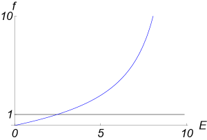
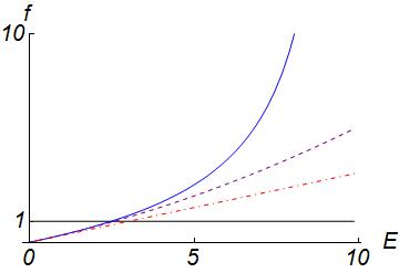
Figure 1: Left panel: Plot of the function $f(E)$ in (17) for the case of the square-well potential. The function $f(E)$ crosses 1 at $E=E^{(0)}=\pi^{2}/4=2.46740$, the ground-state energy, and it becomes infinite at $E=E^{(1)}=\pi^{2}=9.8696$, the radius of convergence of the series. Right panel: Same as the left panel but with the first term (dashed-dotted line) and the first two terms (dashed line) in the power-series expansion of $f(E)$ shown as well. One can see from this graph that just a few terms in the series for $f(E)$ give an accurate numerical approximation to $E^{(0)}$.

We can expand $f(E)$ in (17) as a power series in $E$ and read off the coefficients $a_{k}$:

$$f(E)=\frac{E}{3}+\frac{E^{2}}{45}+\frac{2E^{3}}{945}+\frac{E^{4}}{4725}+\frac{2E^{5}}{93555}+\frac{1382E^{6}}{638512875}+\frac{4E^{7}}{18243225}+\cdots.$$ (18)

Truncating the series for $f(E)$ after $n$ terms and solving numerically for the positive root $E_{n}$ of $f(E)-1$ gives a sequence of approximants $E_{n}$ to the ground-state energy. The first six approximants $E_{1},\,E_{2},\,\ldots,E_{6}$ are listed in Table 1. This table shows that $E_{n}$ converges geometrically to the exact value $E^{(0)}=2.46740$ of the ground-state energy; it is shown in Sec. III that for large $n$ the difference between $E^{(0)}$ and $E_{n}$ approaches 0 like $4^{-n}$.

Order $n$	$E_{n}$	$E_{n}/E^{(0)}$
1	3.0	1.21585
2	2.56231	1.03846
3	2.48906	1.00878
4	2.47267	1.00214
5	2.46871	1.00053
6	2.46773	1.00013

Table 1: First six approximants $E_{n}$ ($n=1,\,2,\,\ldots,6$) to the exact value of the ground-state energy $E^{(0)}=\pi^{2}/4=2.46740$. These approximants are obtained by truncating the expansion of $f(E)-1$ after $n$ terms and finding the positive root $E_{n}$ of the resulting polynomial. The convergence to $E^{(0)}$ is geometric; the error in the $n$th approximant decays to zero like $4^{-n}$.

II.2 Harmonic oscillator $N=2$

For the harmonic-oscillator potential $V(x)=x^{2}$, the function $f(E)$ is

$$f(E)=1-\frac{\Gamma(1/4)\Gamma(3/4-E/4)}{\Gamma(3/4)\Gamma(1/4-E/4)}.$$ (19)

We obtain this result from

$$\psi(x)=\frac{{\rm D}_{(E-1)/2}\big{(}x\sqrt{2}\big{)}}{{\rm D}_{(E-1)/2}(0)},\quad\psi_{0}(x)=\frac{{\rm D}_{-1/2}\big{(}x\sqrt{2}\big{)}}{{\rm D}_{-1/2}(0)}\quad\big{(}E<E^{(1)}=3\big{)},$$

where ${\rm D}_{\nu}(z)$ is the parabolic cylinder function R5 . The power-series expansion of this function gives the coefficients $a_{k}$:

$$f(E)=0.78530E+0.14956E^{2}+0.04403E^{3}+0.01409E^{4}+0.00463E^{5}+0.00153E^{6}+\cdots,$$ (20)

which come from evaluating polylogarithms. As Fig. 2 illustrates, $f(E)$ vanishes at $E=0$, crosses $1$ at the ground-state energy $E^{(0)}=1$ and becomes infinite at $E^{(1)}=3$. Table 2 lists the first six approximants $E_{n}$ to $E^{(0)}$. In Sec. III it is shown that the error vanishes geometrically for large $n$ like $3^{-n}$.

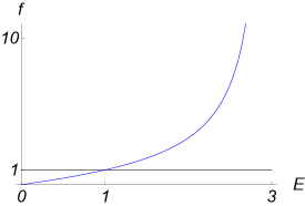
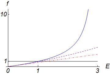
Figure 2: Left panel: Plot of $f(E)$ for the potential $V(x)=x^{2}$ of the quantum harmonic-oscillator. Note that $f(E)=1$ at $E=E^{(0)}=1$ and becomes infinite when $E=E^{(1)}=3$. Right panel: Same as the left panel but with the first two partial sums of the power series expansion for $f(E)$ shown as well. Note that the partial sums converge monotonically upward to $f(E)$.

Order $n$	$E_{n}$
1	1.27324
2	1.05949
3	1.01721
4	1.00543
5	1.00177
6	1.00059

Table 2: First six approximants $E_{n}$ to the ground-state energy $E^{(0)}=1$ of the harmonic oscillator. The error is of order $3^{-n}$.

II.3 Linear potential $N=1$

For the linear potential $V(x)=|x|$, the function $f(E)$ is

$$f(E)=1-\frac{{\rm Ai}(0){\rm Ai}^{\prime}(-E)}{{\rm Ai}^{\prime}(0){\rm Ai}(-E)},$$ (21)

which is derived by substituting $\psi(x)={\rm Ai}(x-E)/{\rm Ai}(-E)$ into (12). The Taylor expansion of this function gives the coefficients $a_{k}$:

$$f(E)=0.72901E+0.15440E^{2}+0.05411E^{3}+0.02131E^{4}+0.00876E^{5}+0.00368E^{6}+\cdots,$$ (22)

which series converges if $E<E^{(1)}$. The function $f(E)$ is plotted in Fig. 2; $f(E)$ crosses $1$ at the ground-state energy $E^{(0)}=1.01879297$ and becomes infinite at $E^{(1)}=2.3381075$. The first six approximants $E_{n}$ to the ground-state energy $E^{(0)}$ are listed in Table 3. It is shown in Sec. III that the error in the $n$th approximant vanishes for large $n$ like $2.295^{-n}$.

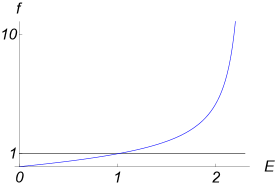
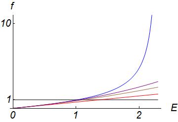
Figure 3: Left panel: Plot of $f(E)$ in (22) for the linear potential $V(x)=|x|$. Note that $f(E)$ passes through $1$ at the ground-state energy $E=^{(0)}1.01879297$ and becomes infinite at $E^{(1)}=2.3381075$. Right panel: Same as left panel but with the first three partial sums in the power-series expansion for $f(E)$ shown as well. Note that the convergence to $f(E)$ is monotone upward and that just a small number of terms in the series gives an accurate value of $E^{(0)}$.

Order $n$	$E_{n}$	$E_{n}/E^{(0)}$
1	1.37172	1.34642
2	1.11052	1.09003
3	1.05136	1.03197
4	1.03168	1.01265
5	1.02415	1.00525
6	1.02107	1.00223

Table 3: First six approximants $E_{n}$ to the ground-state energy of the linear oscillator potential $V(x)=|x|$. The exact value of the ground-state energy is $E^{(0)}=1.01879$. The error in the $n$th approximant is of order $2.295^{-n}$.

II.4 Quartic potential $N=4$

For the quartic potential it is not easy to calculate many terms in the Taylor series expansion of $f(E)$ because it requires the numerical evaluation of multiple integrals. However, the first three terms in this series are

$$f(E)=0.763303E+0.125262E^{2}+0.030303E^{3}+\cdots.$$ (23)

In Table 4 we give the results of calculating the successive zeros of this series.

Order $n$	$E_{n}$	$E_{n}/E^{(0)}$
1	1.31010	1.23552
2	1.10846	1.04536
3	1.07240	1.01136

Table 4: First three approximants to the ground-state energy $1.060362$ of the anharmonic oscillator potential $V(x)=x^{4}$. These approximants are obtained by truncating the series (23).

III Shanks extrapolation

The Shanks transformation R6 is a technique for finding the limit $L$ of a sequence $\{A_{n}\}$ as $n\to\infty$. This technique relies on the assumption that the $n$th term in the sequence has the asymptotic form

$$A_{n}\sim L+cr^{n}\quad(n\to\infty),$$ (24)

where $c$ and $r$ are constants and $|r|<1$. If the asymptotic approximation (24) is accurate, then a simultaneous solution to the three equations

$$A_{n+1}=L+cr^{n+1},\quad A_{n}=L+cr^{n},\quad A_{n-1}=L+cr^{n-1}$$ (25)

gives an accurate value for the limit $L$:

$$L=\frac{A_{n+1}A_{n-1}-A_{n}^{2}}{A_{n+1}+A_{n-1}-2A_{n}}.$$ (26)

Of course, a sequence typically has a more complicated form than the simple three-parameter model in (24), and therefore the value of $L$ in (26) is only approximate. Indeed, this calculation produces a value of $L$ that depends on $n$. However, if the three-parameter model (24) is accurate, then the formula in (26) produces a new sequence

$$\big{\{}\mathcal{S}\big{(}A_{n}\big{)}\big{\}}\equiv\frac{A_{n+1}A_{n-1}-A_{n}^{2}}{A_{n+1}+A_{n-1}-2A_{n}}$$ (27)

that typically converges to the limit $L$ faster than the sequence $\{A_{n}\}$ as $n\to\infty$. The new sequence is called the Shanks transform of the original sequence $\{A_{n}\}$.

The ground-state energy $E^{(0)}$ is the positive solution to the equation $1=f(E)$, where $f(E)$ is given in (12). Let $E_{n}$ be the positive root of the polynomial equation $1=f_{n}(E)$, where $f_{n}(E)$ is the $n$th partial sum of $f(E)$:

$$1=\sum_{k=1}^{n}a_{k}\big{(}E_{n}\big{)}^{k}.$$ (28)

Also, $E_{n+1}$ is the positive root of polynomial equation

$$1=\sum_{k=1}^{n+1}a_{k}\big{(}E_{n+1}\big{)}^{k}.$$ (29)

If we subtract (28) from (29), we obtain the equation

$$0=\sum_{k=1}^{n}a_{k}\left[\big{(}E_{n+1}\big{)}^{k}-\big{(}E_{n}\big{)}^{k}\right]+a_{n+1}\big{(}E_{n+1}\big{)}^{n+1}.$$ (30)

Our numerical studies of $f(E)$, as described in Sec. II, show that for large $n$, $E_{n}$ is approximated very well by the simple Shanks formula

$$E_{n}\sim E^{(0)}+cr^{n}.$$ (31)

Therefore, we can make the approximations

$$\big{(}E_{n}\big{)}^{k} \sim \big{(}E^{(0)}\big{)}^{k}\big{(}1+kcr^{n}/E^{(0)}\big{)},$$

$$\big{(}E_{n+1}\big{)}^{k} \sim \big{(}E^{(0)}\big{)}^{k}\big{(}1+kcr^{n+1}/E^{(0)}\big{)}.$$ (32)

Furthermore, the power series representation for $f(E)$ in (12) has a nonzero radius of convergence, which we denote here by $R$. Thus, for large $n$, we can approximate the $n$th coefficient $a_{n}$ in the series by $KR^{-n}$, where $K$ is a constant. (In addition to this geometric dependence there may also be an algebraic dependence on $n$, but such a dependence does not affect this argument.) Thus, we can approximate the last term in (30) by

$$a_{n+1}\big{(}E_{n+1}\big{)}^{n+1}\sim K\big{(}E^{(0)}\big{)}^{n+1}/R^{n+1}.$$ (33)

These approximations simplify the formula in (30) to

$$(1-r)cr^{n}f^{\prime}\big{(}E^{(0)}\big{)}\sim K\big{(}E^{(0)}\big{)}^{n+1}/R^{n+1}.$$ (34)

Thus, in the limit as $n\to\infty$ we obtain equations for $r$ and $c$:

$$r=E^{(0)}/R,\quad c=\frac{KE^{(0)}}{\big{[}R-E^{(0)}\big{]}f^{\prime}\big{[}E^{(0)}\big{]}}.$$ (35)

Let us apply this analysis in turn to the square-well, harmonic-oscillator, linear, and quartic potentials. For the square-well potential $f(E)$ is given in (17), and we can see from this formula that $E^{(0)}=\pi^{2}/4$ and that $R=E^{(1)}=\pi^{2}$. Thus, (35) implies that $r=1/4$. This explains the observed rate of convergence of the approximants $E_{n}$ in Table 1. If we now compute the Shanks transform $\mathcal{S}\big{[}E_{n}/E^{(0)}\big{]}$ of the entries in the third column in Table 1, we obtain the new improved sequence of approximants $1.00281$, $1.00022$, $1.00002$, $1.00000$, which is a dramatic improvement in accuracy. [Note that the six entries in Table 1 can only give rise to four terms in the Shanks transformed sequence because of the structure of (26).]

For the harmonic-oscillator potential $f(E)$ is given in (19). Thus, $E^{(0)}=1$ and $R=E^{(1)}=3$. Thus, from (35) we see that $r=1/3$. This explains the observed rate of convergence of the approximants $E_{n}$ in Table 2. We compute the Shanks transform of the entries in the second column in Table 2 and we obtain the new improved sequence of approximants $1.00678$, $1.00088$, $1.00012$, $1.00002$, which again is a dramatic improvement in accuracy.

Next, we consider the linear potential; $f(E)$ given in (21). The value of $r=E^{(0)}/E^{(1)}$ is $1/2.29459$, which explains the rate of convergence of the approximants in Table 3. The Shanks transform of the entries in the third column in produces the new and more accurate sequence of approximants $1.01497$, $1.00301$, $1.00066$, $1.00014$.

Finally, we construct the Shanks transform of the three entries in the third column in Table 4 and obtain $1.00396$. This is an improvement in accuracy by a factor of three.

IV Expectation value of $H$

Let us denote by $\Psi_{n}(x)$ the truncation of the series (9) for $\psi(x)$ at order $n$,

$$\Psi_{n}(x)=\psi_{0}(x)\left[1+\sum_{k=1}^{n}E^{k}\phi_{k}(x)\right]$$ (36)

in which we replace $E$ by $E_{n}$ so that $\Psi_{n}(x)$ satisfies the boundary condition $\Psi_{n}^{\prime}(0)=0$. The expectation value $\langle H\rangle_{n}$, of the operator $H$ in the state $\Psi_{n}(x)$ is given by

$$\langle H\rangle_{n}=\frac{1}{\cal N}\int_{0}^{\infty}dx\,\Psi_{n}(x)\left[-\Psi_{n}^{\prime\prime}(x)+x^{N}\Psi_{n}(x)\right],$$ (37)

where ${\cal N}=\int_{0}^{\infty}dx\,\big{[}\Psi_{n}(x)\big{]}^{2}$. Note that we have taken the integration ranges as $(0,\infty)$ rather than $(-\infty,\infty)$ because $\Psi_{n}(x)$ is constructed as an even function when $E=E_{n}$.

Using (3) and the recursion relations (6) for the $\phi_{k}$ we readily find that

$$H\Psi_{n}\equiv-\Psi_{n}^{\prime\prime}+x^{N}\Psi_{n}=E\Psi_{n-1}.$$ (38)

This result reveals the extent to which $\Psi_{n}$ fails to satisfy the Schrödinger equation, for which the right side of this equation would be $E\Psi_{n}$. Using this equation, we get

$$\langle H\rangle_{n}=E_{n}\frac{\int_{0}^{\infty}dx\,\Psi_{n}(x)\Psi_{n-1}(x)}{\int_{0}^{\infty}dx\,\big{[}\Psi_{n}(x)\big{]}^{2}}.$$ (39)

Because all the terms in the expansion of $\psi(x)$ are positive, $\Psi_{n-1}(x)<\Psi_{n}(x)$. Thus, we see that $\langle H\rangle_{n}<E_{n}$. But, the expectation value of $H$ in any approximate eigenfunction must satisfy the inequality $\langle H\rangle_{n}>E_{\rm exact}$. Thus,

$$E_{n}>\langle H\rangle_{n}>E_{\rm exact}.$$ (40)

So, taking the expectation value of $H$ in the state $\Psi_{n}$ is guaranteed to produce a more accurate approximation to $E^{(0)}$ than $E_{n}$. When the $\phi_{k}$ must be calculated as multiple integrals, the maximal dimension of the integrals involved in calculating $\langle H\rangle_{n}$ is $2n+1$, to be compared with $2n-1$ for $E_{n}$. Thus, the maximal dimension, and hence the computational effort, is the same for $\langle H\rangle_{n}$ and $E_{n+1}$. However, we shall see that in every case $\langle H\rangle_{n}$ is much more accurate than $E_{n}$.

Let us now consider in turn the potentials studied in Sec. II and compare $\langle H\rangle_{n}$ with the results given in Tables 1 - 4. For the square well, case A, we have the results that

$$\langle H\rangle_{1}/E_{\rm exact} = 1.001292,$$

$$\langle H\rangle_{2}/E_{\rm exact} = 1.000061,$$

$$\langle H\rangle_{3}/E_{\rm exact} = 1.000003.$$

For the quantum harmonic oscillator, case B, the results are

$$\langle H\rangle_{1} = 1.003921,$$

$$\langle H\rangle_{2} = 1.000343,$$

$$\langle H\rangle_{3} = 1.000035.$$

For the linear potential, case C, we have

$$\langle H\rangle_{1}/E_{\rm exact} = 1.009813,$$

$$\langle H\rangle_{2}/E_{\rm exact} = 1.001427,$$

$$\langle H\rangle_{3}/E_{\rm exact} = 1.019041.$$

Finally, for the anharmonic oscillator, case C, we have

$$\langle H\rangle_{1}/E_{\rm exact} = 1.00202,$$

$$\langle H\rangle_{2}/E_{\rm exact} = 1.00012.$$

These results become more accurate for larger values of the power $N$ of the potential. This may be because the wave functions fall off more rapidly with $x$ as $N$ increases, so the expectation values are less sensitive to the difference in shape between $\Psi_{n}$ and $\Psi_{n-1}$.

V $\mathcal{P}T$-Symmetric Potential $ix^{3}$

Until now we have dealt with real symmetric potentials, $V(-x)=V(x)$, and have exploited the symmetry of the ground-state eigenfunction. The approximate solutions have therefore been required to satisfy the condition $\Psi_{n}^{\prime}(0)=0$. However, our method readily extends to complex ${\cal PT}$-symmetric potentials satisfying $V(-x)=V^{*}(x)$. In particular, it has been shown in a number of papers R7 ; R8 ; R9 that the potentials $V=-(ix)^{N}$ for $N\geq 2$ have a completely real energy spectrum. When $N\geq 2$, the ${\cal PT}$ symmetry is unbroken, that is, the phases of the eigenfunctions can be chosen so that the eigenfunctions are ${\cal PT}$ symmetric, $\psi^{*}(-z)=\psi(z)$. Here, we have written the argument as $z$ because the ${\cal PT}$-symmetric eigenvalue problem can, and for $N\geq 4$ must, be posed on a contour in the complex-$z$ plane lying within an appropriate Stokes wedge R7 . We choose the contour to pass through the origin, and the corresponding condition on the truncated wave functions $\Psi_{n}(z)$ in (36) is

$${\rm Re}\left(\frac{1}{\psi(z)}\frac{d\psi(z)}{dz}\right)_{z=0}=0.$$ (41)

It is convenient to formulate the problem in the right-half plane on the Stokes line $z=\lambda x$, where $\lambda=e^{-i\theta}$ and $\theta=\pi/(2N+4)$. Then for $N=3$ the Schrödinger equation on the Stokes line reads

$$\left(-\frac{d^{2}}{dx^{2}}+x^{3}\right)\psi(x)=\lambda^{2}E\psi(x).$$ (42)

The coefficients in the energy power-series expansion of $\psi(x)$ are the same as those for the potential $V=|x|^{3}$. The only difference between the $ix^{3}$ and the $|x|^{3}$ potentials is that now the expansion is in powers of the complex quantity $\lambda^{2}E$ instead of $E$, where in this case $\theta=\pi/10$.

In terms of $x$ the eigenvalue condition at $z=0$ becomes

$${\rm Re}\left(\frac{1}{\lambda}\frac{1}{\psi(x)}\frac{d\psi(x)}{dx}\right)_{x=0}=0.$$ (43)

Thus,

$$\cos(\theta)\,\frac{\psi^{\prime}_{0}(0)}{\psi_{0}(0)}+\cos(\theta)\,E\phi^{\prime}_{1}(0)+\cos(3\theta)\,E^{2}\phi^{\prime}_{2}(0)+\dots=0.$$ (44)

The principal difference from the Hermitian case is that the coefficient $a_{k}$ in (13) is multiplied by the factor $\cos{(2k-1)\theta}$, which is not positive definite. As a result, some of the coefficients are negative, and other coefficients vanish. This means that convergence of $E_{n}$ to the exact ground-state energy $E^{(0)}$ is no longer monotonic. These features are exemplified by the following numerical results:

$$E_{1}/E^{(0)} = 1.10366,$$

$$E_{2}/E^{(0)} = 0.98258,$$

$$E_{3}/E^{(0)} = E_{2}/E^{(0)}.$$ (45)

The first-order result happens to be the same as for $V=|x|^{3}$ because $\cos(-\theta)=\cos{\theta}$. The second-order result is less than $E^{(0)}$, rather than approaching the exact value from above, and the approximant is unchanged in third order because $\cos(5\theta)=0$.

The reason for choosing the contour as we did is that the integrals over $x$ that are used to construct $\phi_{k}(x)$ and $\phi_{k}^{\prime}(x)$ remain real, and in fact equal those for the Hermitian potential $|x|^{3}$, thus making the evaluation of the coefficients no more difficult than in the Hermitian case. The difference is that in calculating the expectation value of $H$ according to (39), the truncated wave functions $\Psi_{n}$ and $\Psi_{n-1}$ are complex because of the replacement of $E_{n}$ by $\lambda^{2}E_{n}$ in the expansion (2). However, by taking the real parts the integrals can be decomposed into a number of real integrals over the $\phi_{k}(x)$. The results are

$$\langle H\rangle_{1}/E^{(0)} = 0.984,$$

$$\langle H\rangle_{2}/E^{(0)} = 0.997.$$ (46)

Again, both $\langle H\rangle_{1}$ and $\langle H\rangle_{2}$ are less than the true value $E^{(0)}$ but closer than $E_{2}$ and $E_{3}$, respectively. Recall that $\langle H\rangle_{n}$ and $E_{n+1}$ require about the same calculational effort.

In summary, we can see that while the results do converge to the ground-state energy, the convergence is not as rapid as for the corresponding Hermitian potential $V=|x|^{N}$. This is not surprising considering the very similar variational results in Ref. R10 , where high-dimensional matrices were diagonalized to obtain the numerical approximations to the eigenvalues.

VI Padé calculation of higher energy levels

As explained in Sec. I, one can find the approximate poles and zeros of $f(E)-1$ by converting (14) to the diagonal sequence of Padé approximants. The poles give approximations to the odd-parity eigenvalues, while the zeros give approximations to the even-parity eigenvalues. In Tables 5-7 below we list the first four eigenvalues obtained from the Padé approximants $P_{1}^{1}$, $P_{2}^{2}$, $P_{3}^{3}$, and $P_{4}^{4}$ for the potentials considered in Subsecs. II.1-II.3.

Energy	$P_{1}^{1}$	$P_{2}^{2}$	$P_{3}^{3}$	$P_{4}^{4}$	Exact
$E^{(0)}$	$2.50000$	$2.46744$	$2.46740$	$2.46740$	$2.46740$
$E^{(1)}$	—	$9.94122$	$9.86993$	$9.86960$	$9.86960$
$E^{(2)}$	—	—	$22.29341$	$22.20737$	$22.20661$
$E^{(3)}$	—	—	—	$39.56379$	$39.47842$

Table 5: Energies obtained from the first four diagonal Padé approximants for the square-well potential $V(x)=0$ ($|x|\leq 1)$, $V(x)=\infty$ ($|x|>1$).

Energy	$P_{1}^{1}$	$P_{2}^{2}$	$P_{3}^{3}$	$P_{4}^{4}$	Exact
$E^{(0)}$	$1.02478$	$1.00013$	$1.00000$	$1.00000$	$1$
$E^{(1)}$	—	$3.08260$	$3.00237$	$3.00003$	$3$
$E^{(2)}$	—	—	$5.12647$	$5.00701$	$5$
$E^{(3)}$	—	—	—	$7.16012$	$7$

Table 6: Energies obtained from the first four diagonal Padé approximants for the harmonic oscillator potential $V(x)=x^{2}$.

Energy	$P_{1}^{1}$	$P_{2}^{2}$	$P_{3}^{3}$	$P_{4}^{4}$	Exact
$E^{(0)}$	$1.06291$	$1.01948$	$1.01880$	$1.01879$	$1.01879$
$E^{(1)}$	—	$2.48513$	$2.34902$	$2.33863$	$2.33811$
$E^{(2)}$	—	—	$3.44920$	$3.27292$	$3.24820$
$E^{(3)}$	—	—	—	$4.35282$	$4.08795$

Table 7: Energies obtained from the first four diagonal Padé approximants for the linear potential $V(x)=|x|$.

For the anharmonic oscillator potential $V(x)=x^{4}$ we have only calculated the series for $f(E)$ in (23) to third order in powers of $E$. If we use the diagonal Padé approximant $P_{1}^{1}$, we obtain the estimate $E^{(0)}=1.07827$, which is accurate to about 2% and is a slight improvement on the second entry in Table 4. However, the Padé approximant $P_{1}^{2}$ gives $E^{(0)}=1.06137$, a significant improvement in numerical accuracy (one part in a thousand) compared with the results in Table 4. This Padé approximant also gives the value $4.13364$ for the first excited state, which differs from the exact value $3.79967$ by about 9%.

VII BRIEF COMMENTS

In this paper we have shown how to construct a perturbative solution to the time-independent Schrödinger equation $-\psi^{\prime\prime}(x)+V(x)\psi(x)=E\psi(x)$ [$V(x)$ even] as a formal series in powers of the energy $E$ itself. We have then used this expansion to obtain remarkably accurate numerical approximations to the ground-state energy, and also to the higher energy levels by the use of various numerical methods such as the Shanks transformation and Padé approximation. The surprise is that even though the energy levels of the quantum theory are not small compared with 1, the perturbation expansion is convergent if $E<E^{(1)}$, the first energy level. Furthermore, the perturbation expansion that we have constructed can also be applied to non-Hermitian $\mathcal{P}T$-symmetric potentials. Our general approach has been to solve the unperturbed problem $-\psi_{0}(^{\prime\prime}x)+V(x)\psi_{0}(x)=0$ for $x\geq 0$ and to use $\psi_{0}(x)$ as the building block for constructing $\psi(x)$ for $x\geq 0$ as a perturbative expansion in $E$. The approximate eigenvalues are then obtained by the condition that $\psi(x)$ can be extended by parity (or $\mathcal{P}T$-symmetry) to negative $x$. In the future, we plan to extend the techniques developed here to quantum theories in higher-dimensional space.

Finally, in the present paper we have limited ourselves to providing an elementary, accurate, and general recipe for calculating the low-lying eigenvalues of symmetric or $\mathcal{P}T$-symmetric potentials using simple analytical and numerical tools. The recipe essentially provides a method of calculating the truncated Weierstrass products for $\psi^{\prime}(0)$ and $\psi(0)$. Hence it may be interesting to explore further the connection of the method to such topics as spectral zeta functions, functional determinants and infinite products of eigenvalues [11].

References

• (1) See, for example, E. Merzbacher, Quantum Mechanics (John Wiley and Sons, New York, 1970), 2nd edition.
• (2) J. L. Dunham, Phys. Rev. 41, 713 (1932).
• (3) C. M. Bender, K. Olaussen, and P. S. Wang, Phys. Rev. D 16, 1740 (1977).
• (4) C. M. Bender and S. A. Orszag, Advanced Mathematical Methods for Scientists and Engineers (McGraw Hill, New York, 1978), Chap. 10.
• (5) I. S. Gradshteyn and I. M. Ryzhik, Table of Integrals, Series, and Products (Academic, New York, 1965).
• (6) See Ref. R4 , Chap. 8.
• (7) C. M. Bender and S. Boettcher, Phys. Rev. Lett. 80, 5243 (1998).
• (8) P. E. Dorey, C. Dunning, and R. Tateo, J. Phys. A: Math. Gen. 34, L391 (2001) and 34, 5679 (2001).
• (9) P. E. Dorey, C. Dunning, and R. Tateo, J. Phys. A: Math. Gen. 40, R205 (2007).
• (10) C. M. Bender and D. J. Weir, J. Phys. A: Math. Theor. 45, 425303 (2012).
• (11) See, for example, S. Levit and U. Smilansky, Proc. Am. Math. Soc. 65, 299 (1977).