Phase transitions and sample complexity in Bayes-optimal matrix factorization

Abstract

We analyse the matrix factorization problem. Given a noisy measurement of a product of two matrices, the problem is to estimate back the original matrices. It arises in many applications such as dictionary learning, blind matrix calibration, sparse principal component analysis, blind source separation, low rank matrix completion, robust principal component analysis or factor analysis. It is also important in machine learning: unsupervised representation learning can often be studied through matrix factorization. We use the tools of statistical mechanics – the cavity and replica methods – to analyze the achievability and computational tractability of the inference problems in the setting of Bayes-optimal inference, which amounts to assuming that the two matrices have random independent elements generated from some known distribution, and this information is available to the inference algorithm. In this setting, we compute the minimal mean-squared-error achievable in principle in any computational time, and the error that can be achieved by an efficient approximate message passing algorithm. The computation is based on the asymptotic state-evolution analysis of the algorithm. The performance that our analysis predicts, both in terms of the achieved mean-squared-error, and in terms of sample complexity, is extremely promising and motivating for a further development of the algorithm .

I Introduction

We study in this paper a variety of questions which all deal with the general problem of matrix factorization. Generically, this problem is stated as follows: Given a $M\times P$ dimensional matrix $Y$, that was obtained from noisy element-wise measurements of a matrix $Z$, one seeks a factorization $Z=FX$, where the $M\times N$ dimensional matrix $F$ and the $N\times P$ dimensional matrix $X$ must satisfy some specific requirements like sparsity, low-rank or non-negativity.

From a machine learning point of view, matrix factorization can be applied to unsupervised learning of data representation Bengio et al. (2013). The success of machine learning, including recent progress such as deep learning LeCun et al. (2015), depends largely on data representations. Explicit approaches to efficient data representation, such as matrix factorization, are hence of wide relevance. Other applications that can be formulated as matrix factorization include dictionary learning or sparse coding Olshausen et al. (1996); Olshausen & Field (1997); Kreutz-Delgado et al. (2003), sparse principal component analysis Zou et al. (2006), blind source separation Belouchrani et al. (1997), low rank matrix completion Candès & Recht (2009); Candès & Tao (2010) or robust principal component analysis Candès et al. (2011), that will be described below.

Theoretical limits on when matrix factorization is possible and computationally tractable are still rather poorly understood. In this work we make a step towards this understanding by predicting the limits of matrix factorization and its algorithmic tractability when $Z$ is created using randomly generated matrices $F$ and $X$, and measured element-wise via a known noisy output channel $P_{\rm out}(Y|Z)$. Our results are derived in the limit where $N,M,P\to\infty$ with fixed ratios $M/N=\alpha$, $P/N=\pi$. We predict the existence of sharp phase transitions in this limit and provide the explicit formalism to locate them.

We use two types of methods in this paper. The first one is based on a generalization of approximate message passing (AMP) Donoho et al. (2009) to the matrix factorization problem, and on its asymptotic analysis which is known in statistical physics as the cavity method Mézard et al. (1987); Mézard & Montanari (2009), and has been called state evolution in the context of compressed sensing Donoho et al. (2009). The second method that we use in the following is the replica method. These two methods are widely believed to be exact in the context of theoretical statistical physics, but most of the results that we shall obtain in the present work are not rigorously established. Our predictions have thus the status of conjectures. A first cross-check of the correctness of these conjectures is the fact that the two methods give identical results. This has been understood first in the context of spin glasses Mézard et al. (1987).

This work builds upon some previous steps that we described in earlier reports Sakata & Kabashima (2013); Krzakala et al. (2013). The message passing algorithm related to our analysis was first presented in Krzakala et al. (2013) and is very closely related to the Big-AMP algorithm developed and tested in Schniter et al. (2012); Parker et al. (2013, 2014); relations and differences with Big-AMP will be mentioned in several places throughout the paper. Our main focus here, beside the detailed derivation of the algorithm, is the asymptotic analysis and phase diagrams which were not studied in Schniter et al. (2012); Parker et al. (2013, 2014). We also discuss several variants of the AMP algorithm that are interesting for theoretical reasons. Several of these variants, however, have convergence problems when implemented straightforwardly. For a robust implementation of the algorithm that can be used on practical benchmarks we refer to the works Parker et al. (2013, 2014).

Our general method provides a unifying framework for the study of computational tractability and identifiability of various matrix factorization problems. The first step for this synergy is the formulation of the problem via a graphical model (see Fig. 1) that is amenable to analysis using the present methods.

The phase diagrams that we shall derive establishes for each problem two types of thresholds in the plane $\alpha-\pi$ : the threshold where the problem of matrix factorization ceases to be solvable in principle, and the threshold where AMP ceases to find the best solution. In most existing works the computation of phase transitions was treated separately for each of the various problems. For instance, redundant dictionaries for sparse representations and low rankness are usually thought as two different kinds of dimensional reduction. Interestingly, in our work a wide class of problems is treated within one unified formalism; this is theoretically interesting in the context of recent developments Elad (2012).

I.1 Statement of the problem

In a general matrix factorization problem one measures some information about matrix elements of the product of two unknown matrices $F\in{\mathbb{R}}^{M\times N}$ and $X\in{\mathbb{R}}^{N\times P}$, whose matrix elements will be denoted $F_{\mu i}$ and $X_{il}$. Let us denote the product $Z=FX\in{\mathbb{R}}^{M\times P}$, with elements

$$z_{\mu l}=\sum_{i=1}^{N}F_{\mu i}X_{il}\,.$$ (1)

The element-wise measurement $y_{\mu l}$ of $z_{\mu l}$ is then specified by some known probability distribution function $P_{\rm out}(y_{\mu l}|z_{\mu l})$, so that:

$$P_{\rm out}(Y|Z)=\prod_{\mu,l}P^{\mu l}_{\rm out}(y_{\mu l}|z_{\mu l})\,.$$ (2)

The goal of matrix factorization is to estimate both matrices $F$ and $X$ from the measurements $Y$.

In this paper we will treat this problem in the framework of Bayesian inference. In particular we will assume that the matrices $F$ and $X$ were both generated from a known separable probability distribution

$$P_{F}(F) = \prod_{\mu=1}^{M}\prod_{i=1}^{N}P^{\mu i}_{F}(F_{\mu i})\,,$$ (3)

$$P_{X}(X) = \prod_{i=1}^{N}\prod_{l=1}^{P}P^{il}_{X}(X_{il})\,.$$ (4)

Although we restrict to separable prior probability distributions $P_{F}(F)$, $P_{X}(X)$, it turns out that these priors can encode a broad range constraints such as, for instance sparsity. This is the reason why so many different problems can be studied within our scheme. The output channel $P_{\rm out}(y,z)$ can be of a rather generic nature, thus including various kinds of additive and multiplicative noise; in the spirit of activation functions from neural networks it can degrade the information included in the measurement by e.g. keeping only the sign of elements of $z$.

In the following we shall mostly study the case where the distributions $P^{\mu i}_{F}$ are all identical (there is a single distribution $P_{F}(F_{\mu i})$), and the distributions $P^{il}_{X}$ for various $il$ (as well as $P_{\rm out}^{\mu l}$ for various $\mu l$) are also all identical. Our approach can be generalized to the case where $P^{\mu i}_{F}$, $P^{il}_{X}$, $P_{\rm out}^{\mu l}$ depend in a known way on the indices $\mu i$, $il$, and $\mu l$, provided that this dependence is through parameters that themselves are taken from separable probability distributions. Examples of such dependence include the blind matrix calibration or the factor analysis. On the other hand our theory does not cover the case of an arbitrary matrix $\tilde{F}_{\mu i}$ for which we would have $P_{F}^{\mu i}=\delta(F_{\mu i}-\tilde{F}_{\mu i})$.

The posterior distribution of $F$ and $X$ given the measurements $Y$ is written as

$$P(F,X|Y)=\frac{1}{{\cal Z}(Y)}P_{F}(F)P_{X}(X)P_{\rm out}(Y|FX)=\frac{1}{{\cal Z}(Y)}\prod_{\mu,i}P_{F}(F_{\mu i})\prod_{i,l}P_{X}(X_{il})\prod_{\mu,l}P_{\rm out}\left(y_{\mu l}|\sum_{i}F_{\mu i}X_{il}\right)\,,$$ (5)

where ${\cal Z}(Y)$ is the normalization constant, known as the partition function in statistical physics.

Notice that, while the original problem of finding $F$ and $X$, given the measurements $Y$, is not well determined (because of the possibility to obtain, from a given solution, an infinity of other solutions through the transformation $F\to FU^{-1}$ and $X\to UX$, where $U$ is any $N\times N$ nonsingular matrix), the fact of using well defined priors $P^{\mu i}_{F}$ and $P^{il}_{X}$ actually lifts the degeneracy: the problem of finding the most probable $F,X$ given the measurements and the priors is well defined. In case the priors $P^{\mu i}_{F}$ and $P^{il}_{X}$ do not depend on the indices $\mu l$ and $il$ we are left with a permutational symmetry between the $N$ column of $F$ and $N$ rows of $X$. Both in the algorithm and the asymptotic analysis this symmetry is broken and one of the $N\!$ solutions is chosen at random.

Typically, in most applications, the distributions $P_{\rm out}$, $P_{F}$ and $P_{X}$ will depend on a set of parameters (such as the mean, variance, sparsity, noise strength, etc.) that we usually will not write explicitly in the general case, in order to simplify the notations. The prior knowledge of these parameters is not necessarily required in our approach: these parameters can be learned via an expectation-maximization-like algorithm that we will discuss briefly in section II.5.

Note also that Eq. 1 can be multiplied by an arbitrary constant: with a corresponding change in the output function the problem will not be modified. In the derivations of this paper we choose the above constant in such a way that the elements of matrices $X$, $Y$, and $Z$ are of order $O(1)$, whereas the elements of $F$ scale in a consistent way, meaning that the mean of each $F_{\mu i}$ is of order $O(1/N)$ and its variance is also of order $O(1/N)$.

I.2 Bayes-optimal inference

Our paper deals with the general case of incomplete information. This happens when the reconstruction assumes that the matrices $X$, $F$ and $Y$ were generated with some distributions $P_{X}$, $P_{F}$ and $P_{\rm out}(Y|Z)$, whereas in reality the matrices were generated using some other distributions $P_{X^{0}}$, $P_{F^{0}}$ and $P^{0}_{\rm out}(Y|Z)$. The message passing algorithm and its asymptotic evolution will be derived in this general case.

However, our most important results concern the Bayes-optimal setting, i.e. when we assume that

$$P_{X^{0}}=P_{X},\quad\quad P_{F^{0}}=P_{F},\quad\quad P^{0}_{\rm out}(Y|Z)=P_{\rm out}(Y|Z)\,.$$ (6)

In this case, an estimator $X^{\star}$ that minimizes the mean-squared error (MSE) with respect to the original signal $X^{0}$, defined as

$${\rm MSE}(X|Y)=\int\text{d}F^{0}\,\text{d}X^{0}\left[\frac{1}{PN}\sum_{il}(X_{il}-X^{0}_{il})^{2}\right]P(F^{0},X^{0}|Y)\,,$$ (7)

is obtained from marginals of $X_{il}$ with respect to the posterior probability measure $P(F,X|Y)$, i.e.,

$$X^{\star}_{il}=\int\text{d}X_{il}\,X_{il}\,\nu_{il}(X_{il})\,,\quad\quad{\rm where}\quad\quad\nu_{il}(X_{il})\equiv\int_{\{F_{\mu j}\}}\int_{\{X_{jn}\}_{jn\neq il}}P(F,X|Y)\,,$$ (8)

is the marginal probability distribution of the variable $il$. The mean squared error achieved by this optimal estimator is called the minimum mean squared error (MMSE) in this paper.

A similar result holds for the estimator of $F^{0}$ that minimizes the mean-squared error

$${\rm MSE}(F|Y)=\int\text{d}F^{0}\,\text{d}X^{0}\left[\frac{1}{M}\sum_{\mu i}(F_{\mu i}-F^{0}_{\mu i})^{2}\right]P(F^{0},X^{0}|Y)\,,$$ (9)

which is obtained from the mean of $F_{\mu i}$ with respect to the posterior probability measure $P(F,X|Y)$. In the remainder of this article we will be using these estimators.

I.3 Statement of the main result

The main result of this paper are explicit formulas for the MMSE achievable in the Bayes optimal setting (as defined above) for the matrix factorization problem in the “thermodynamic limit”, i.e. when $N,M,P\to\infty$ with fixed ratios $M/N=\alpha$, $P/N=\pi$. When sparsity is involved we consider that a finite fraction of matrix elements are non-zero. Similarly, when we treat matrices with low ranks we consider again the ranks to be a finite fraction of the total dimension. We also derive the AMP-MSE, i.e. the mean square error achievable by the approximate message passing algorithm as derived in this paper.

So far we were characterizing the output channel by the conditional distribution $P^{0}_{\rm out}(y|z^{0})$ or $P_{\rm out}(y|z)$. It will be useful to think of the output as a deterministic function $h$ of $z$ and of random variables $w$, i.e. $y_{\mu l}=h(z_{\mu l},w_{\mu l})=h^{0}(z^{0}_{\mu l},w_{\mu l}^{0})$. The random (“noise”) variables $w$ and $w^{0}$ are specified by their probability distributions $P(w)$ and $P_{0}(w^{0})$. We can relate $P_{\rm out}$ to $h$ as follows

$$P_{\rm out}(y|z) = \int P(w)\,{\rm d}w\,\delta[y-h(z,w)]\,,$$ (10)

$$P^{0}_{\rm out}(y|z^{0}) = \int P_{0}(w^{0})\,{\rm d}w^{0}\,\delta[y-h^{0}(z^{0},w^{0})]\,,$$ (11)

To compute the MMSE and AMP-MSE we need to analyze the fixed points of the following iterative equation.

$$m_{X}^{t+1} = \int{\rm d}XP_{X}(X)\int{\cal D}\xi\,\,f_{X}^{2}\left[\frac{1}{\alpha m_{F}^{t}\hat{m}^{t}},\frac{\alpha m_{F}^{t}\hat{m}^{t}\,X+\xi\sqrt{\alpha m_{F}^{t}\hat{m}^{t}}}{\alpha m_{F}^{t}\hat{m}^{t}}\right]\,,$$ (12)

$$m_{F}^{t+1} = \int{\rm d}FP_{F}(F)\int{\cal D}\xi\,\,f_{F}^{2}\left[\frac{1}{\pi m_{X}^{t}\hat{m}^{t}},\frac{\pi m_{X}^{t}\hat{m}^{t}\,\sqrt{N}F+\xi\sqrt{\pi m_{X}^{t}\hat{m}^{t}}}{\pi m_{X}^{t}\hat{m}^{t}}\right]\,,$$ (13)

$$\hat{m}^{t} = -\int{\rm d}w\,P(w)\int{\rm d}p\,{\rm d}z\frac{e^{-\frac{p^{2}}{2m_{F}^{t}m_{X}^{t}}}e^{-\frac{(z-p)^{2}}{2[\langle(z^{0})^{2}\rangle-m_{F}^{t}m_{X}^{t}]}}}{2\pi\sqrt{m_{F}^{t}m_{X}^{t}(\langle(z^{0})^{2}\rangle-m_{F}^{t}m_{X}^{t})}}\,\partial_{p}g_{\rm out}(p,h(z,w),\langle(z^{0})^{2}\rangle-m_{F}^{t}m_{X}^{t})\,,$$ (14)

where ${\cal D}\xi$ is a notation for a Gaussian probability measure ${\rm d}\xi e^{-\xi^{2}/2}/\sqrt{2\pi}$. We denoted $\langle(z^{0})^{2}\rangle=N\mathbb{E}[(F^{0})^{2}]\mathbb{E}[(X^{0})^{2}]$. Here $f_{X}$ and $f_{F}$ are the so-called input functions, they are defined using the prior distributions $P_{X}$ and $P_{F}$ as

$$f_{X}(\Sigma,T) \equiv \frac{\int{\rm d}X\,XP_{X}(X)e^{-\frac{(X-T)^{2}}{2\Sigma}}}{\int{\rm d}X\,P_{X}(X)e^{-\frac{(X-T)^{2}}{2\Sigma}}}$$ (15)

$$f_{F}(Z,W) \equiv \sqrt{N}\frac{\int{\rm d}F\,FP_{F}(F)e^{-\frac{(\sqrt{N}F-W)^{2}}{2Z}}}{\int{\rm d}F\,P_{F}(F)e^{-\frac{(\sqrt{N}F-W)^{2}}{2Z}}}\,.$$ (16)

The output function $g_{\rm out}$ is defined using the output probability $P_{\rm out}$ as

$$g_{\rm out}(\omega,y,V)\equiv\frac{\int{\rm d}zP_{\rm out}(y|z)\,(z-\omega)\,e^{-\frac{(z-\omega)^{2}}{2V}}}{V\int{\rm d}zP_{\rm out}(y|z)e^{-\frac{(z-\omega)^{2}}{2V}}}\,.$$ (17)

The MSE is computed as ${\rm MSE}_{F}=\mathbb{E}[(F^{0})^{2}]-m_{F}$ and ${\rm MSE}_{X}=\mathbb{E}[(X^{0})^{2}]-m_{X}$ with $m_{F}$ and $m_{X}$ being fixed points of (12-14).

The AMP-MSE is obtained from a fixed point reached with a so-called uninformative initialization. The uninformative initialization does not use any information about the seeked matrices $F^{0},X^{0}$, it uses only the prior distributions, it is defined as

$$m_{F}^{t=0}=N\mathbb{E}[F]^{2}\,,\quad\quad m_{X}^{t=0}=\mathbb{E}[X]^{2}\,.$$ (18)

In case the prior distribution depends on another random variables, e.g. in case of matrix calibration, we take additional average with respect to that variable. If the above initialization gives $m_{F}^{t=0}=0$ and $m_{X}^{t=0}=0$ then this is a fixed point of the above iterative equations. This is due to the permutational symmetry between the columns of matrix $F$ and rows of matrix $X$. To obtain a nontrivial fixed point we initialize at $m_{F}^{t=0}=\eta$ for some very small $\eta$, corresponding to an infinitesimal prior information about the matrix elements of the matrix $F$.

To compute the MMSE we need to initialize the iterations in an informative way, using the knowledge of the true $X^{0}$ and $F^{0}$. This informative initialization is defined as an infinitesimal perturbation of

$$m^{t=0}_{F}=N\mathbb{E}[(F^{0})^{2}]\,,\quad\quad m^{t=0}_{X}=\mathbb{E}[(X^{0})^{2}]\,.$$ (19)

If the resulting fixed point agrees with the AMP-MSE then this is also the MMSE. In case that this informative initialization leads to a different fixed point than the AMP-MSE then the MMSE is given by the one of them for which the following free entropy is larger

$$\phi(m_{F},m_{X},\hat{m}_{F}=\pi m_{X}\hat{m},\hat{m}_{X}=\alpha m_{F}\hat{m})=$$ (20)

$$\alpha\pi\int{\rm d}y\,{\cal D}\xi\,{\cal D}u^{0}P_{\rm out}\left(y|\sqrt{Q_{F}^{0}Q_{X}^{0}-m_{F}m_{X}}u^{0}+{\sqrt{m_{F}m_{X}}}\xi\right)\log\left(\int{\cal D}u\,P_{\rm out}\left(y|\sqrt{Q_{F}^{0}Q_{X}^{0}-m_{F}m_{X}}u+\sqrt{m_{F}m_{X}}\xi\right)\right)$$

$$+\alpha\left(-\frac{\hat{m}_{F}m_{F}}{2}+\int{\cal D}\xi\,{\rm d}F^{0}e^{-\frac{N\hat{m}_{F}}{2}(F^{0})^{2}+\sqrt{N\hat{m}_{F}}\xi F^{0}}P_{F}(F^{0})\log\left(\int{\rm d}Fe^{-\frac{N\hat{m}_{F}}{2}F^{2}+\sqrt{N\hat{m}_{F}}\xi F}P_{F}(F)\right)\right)$$

$$+\pi\left(-\frac{\hat{m}_{X}m_{X}}{2}+\int{\cal D}\xi\,{\rm d}X^{0}e^{-\frac{\hat{m}_{X}}{2}(X^{0})^{2}+\sqrt{\hat{m}_{X}}\xi X^{0}}P_{X}(X^{0})\log\left(\int{\rm d}Xe^{-\frac{\hat{m}_{X}}{2}X^{2}+\sqrt{\hat{m}_{X}}\xi X}P_{X}(X)\right)\right),$$

Sections III, IV, V are devoted to the derivation of these formulas for MMSE and AMP-MSE. In section VI we then give a number of examples of phase diagram for specific applications of the matrix factorization problem.

We reiterate at this point that whereas our results are exact results within the theoretical physics scope of the cavity/replica method, we do not provide their proofs and their mathematical status is that of conjectures. We devote section II.3 to explaining the reasons of why this is so. The situation is comparable to the predictions-conjectures that were made for the satisfiability threshold Mézard et al. (2002), which have been partly established rigorously recently Ding et al. (2014), or the predictions-conjectures that were made for the CDMA problem Tanaka (2002); Guo & Verdú (2005), and were later proved by Montanari & Tse (2006); Bayati & Montanari (2011).

I.4 Applications of matrix factorization

Several important problems which have received a lot of attention recently are special cases of the matrix factorization problem as set above. In this paper we will analyse the following ones.

Dictionary learning.

This is a basic example of finding a representation of data that is advantageous in some way. Representation learning Bengio et al. (2013) is a concept behind many machine learning applications, including the deep learning framework which has become very popular in recent time LeCun et al. (2015). In the context of representation learning dictionary learning is sometimes referred to as sparse coding Bengio et al. (2013).

Dictionary learning relies on the fact that signals of interest are often sparse in some basis; this property is widely used in data compression and more recently in compressed sensing. A lot of work has been devoted to analyzing bases in which different data are sparse. The goal of dictionary learning is to infer a basis in which the data are sparse based purely on a large number of samples from the data. The $M\times P$ matrix $Y$ then represents the $P$ samples of $M$-dimensional data. The goal is to decompose $Y=FX+W$ into a $M\times N$ matrix $F$, and a $N\times P$ sparse matrix $X$, $W$ is the noise.

In this paper we will analyse the following teacher-student scenario of dictionary learning. We will generate a random Gaussian matrix $F^{0}$ with iid elements of zero mean and variance $1/N$, and a random Gauss-Bernoulli matrix $X^{0}$ with fraction $0<\rho<1$ of non-zero elements. The non-zero elements of $X^{0}$ will be iid Gaussian with mean $\overline{X}$ and variance $\sigma$. The noise $W^{0}$ with elements $w^{0}_{\mu l}$ is also iid Gaussian with zero mean and variance $\Delta$. We hence have

$$P_{F}(F_{\mu i}) = P_{F^{0}}(F_{\mu i})=\frac{1}{\sqrt{2\pi/N}}e^{-\frac{NF^{2}_{\mu i}}{2}}\,,$$ (21)

$$P_{X}(X_{il}) = P_{X^{0}}(X_{il})=(1-\rho)\delta(X_{il})+\frac{\rho}{\sqrt{2\pi\sigma}}e^{-\frac{(X_{il}-\overline{X})^{2}}{2\sigma}}\,,$$ (22)

$$P_{\rm out}(y_{\mu l}|z_{\mu l}) = \frac{1}{\sqrt{2\pi\Delta}}e^{-\frac{(y_{\mu l}-z_{\mu l})^{2}}{2\Delta}}\,,$$ (23)

where $\delta(X)$ is the Dirac delta function. The goal is to infer $F^{0}$ and $X^{0}$ from the knowledge of $Y$ with the smallest possible number of samples $P$.

In the noiseless case, $\Delta=0$, exact reconstruction might be possible only when the observed information is larger that the information that we want to infer. This provides a simple counting bound on the number of needed samples $P$:

$$P\geq\frac{\alpha}{\alpha-\rho}N\,.$$ (24)

Note that the above assumptions on $P_{F}$, $P_{X}$ and $P_{\rm out}$ likely do not hold in any realistic problem. However, it is of theoretical interest to analyze the average theoretical performance and computational tractability of such a problem, as it gives a well defined benchmark. Moreover, we anticipate that if we develop an algorithm working well in the above case it might also work well in many real applications where the above assumptions are not satisfied, in the same spirit as the approximated message passing algorithm derived for compressed sensing with zero mean Gaussian measurement matrices Donoho et al. (2009) works also for other kinds of matrices.

Typically, we would look for an invertible basis $F^{0}$ with $N=M$, in that case we speak of a square dictionary. However, with the compressed-sensing application in mind, it is also very interesting to consider that $Y$ might be under-sampled measurements of the actual signal, corresponding then to $\alpha=M/N<1$. Hence we will be interested in the whole range $0<\alpha\leq 1$. The regime of $\alpha<1$ corresponds to an overcomplete dictionary, in which case each of the $P$ measurements $\vec{y}_{l}$ is a sparse linear combination of the columns (atoms) of the dictionary.

We remind that the $N$ columns of the matrix $F^{0}$ can always be permuted arbitrarily and multiplied by $\pm 1$. This is also true for rows of the matrix $X^{0}$: all these operations do not change $Y$, nor the posterior probability distribution. This is hence an intrinsic freedom in the dictionary learning problems that we have to keep in mind. Note that many works consider the dictionary to be column normalized, which lifts part of the degeneracy in some optimization formulations of the problem. In our setting the equivalent of column normalization is asymptotically determined by the properties of the prior distribution.

Blind matrix calibration.

In dictionary learning one does not have any specific information about the elements $F^{0}_{\mu i}$. However in some applications of compressed sensing one might have an approximate knowledge of the measurement matrix: it is often possible to use known samples of the signal $X$ in order to calibrate the matrix in a supervised manner (i.e. using known training samples of the signal). Sometimes, however, the known training samples are not available and hence the only way to calibrate is to measure a number of unknown samples and perform their reconstruction and calibration of the matrix at the same time, such a scenario is called the blind calibration.

In blind matrix calibration, the properties of the signal and the output function are the same as in dictionary learning, eqs. (22-23). As for the matrix elements $F^{0}_{\mu i}$ one knows a noisy estimation $F^{\prime}_{\mu i}$. In this work we will assume that this estimation was obtained from $F^{0}_{\mu i}$ as follows

$$F^{\prime}_{\mu i}=\frac{F^{0}_{\mu i}+\sqrt{\eta}\xi_{\mu i}}{\sqrt{1+\eta}}\,,$$ (25)

where $\xi_{\mu i}$ is a Gaussian random variables with zero mean and variance $1/N$. This way, if the matrix elements $F^{0}_{\mu i}$ have zero mean and variance $1/N$, then the same is true for the elements $F^{\prime}_{\mu i}$.

The control parameter $\eta$ is then quantifying how well one knows the measurement matrix. It provides a way to interpolate between the pure compressed sensing $\eta=0$, where one knows the measurement matrix $F^{0}$, and the dictionary learning problems $\eta\to\infty$. Explicitly, the prior distribution of a given element of the matrix $F$ is

$$P_{F}(F_{\mu i})={\cal N}\left(\frac{F^{\prime}_{\mu i}}{\sqrt{1+\eta}},\frac{\eta}{N(1+\eta)}\right)\ ,$$ (26)

where ${\cal N}(a,b)$ is a Gaussian distribution with mean $a$ and variance $b$.

Low-rank matrix completion

Another special case of matrix factorization that is often studied is the low-rank matrix completion. In that case one “knows” only a small (but in our case finite when $N\to\infty$) fraction $\epsilon$ of elements of the $M\times P$ matrix $Y$. Also one knows which elements are known and which are not; let us call ${\cal M}$ the set on which elements are known, it is a set of size $\epsilon MP$. In this case the output function is:

$$P_{\rm out}(y_{\mu l}|z_{\mu l}) = \frac{1}{\sqrt{2\pi\Delta}}e^{-\frac{(y_{\mu l}-z_{\mu l})^{2}}{2\Delta}}\quad{\rm if}\quad\mu l\in{\cal M}\ ,$$ (27)

$$= \frac{1}{\sqrt{2\pi}}e^{-\frac{y_{\mu l}^{2}}{2}}\quad{\rm if}\quad\mu l\notin{\cal M}\,.$$

The precise choice on the function on the second line is arbitrary as long as it does not depend on the $z_{\mu l}$. In what follows we will assume that the $\epsilon MP$ known elements were chosen uniformly at random.

In low rank matrix completion $N$ is small compared to $M$ and $P$, hence both $\pi$ and $\alpha$ are relatively large. Note, however, that the limit we analyse in this paper keeps $\pi=O(1)$ and $\alpha=O(1)$ while $N\to\infty$, whereas in many previous works on low-rank matrix completion the rank was considered to be $O(1)$ and hence $\alpha$ and $\pi$ of order $O(N)$. Compared to those works the analysis here applies to “not-so-low-rank” matrix completion. The question is what fraction $\epsilon$ of elements of $Y$ needs to be known in order to be able to reconstruct the two matrices $F^{0}$ and $X^{0}$.

For negligible measurement noise, $\Delta=0$, a simple counting bound gives that the fraction of known elements we need for reconstruction is at least

$$\epsilon\geq\frac{\alpha+\pi}{\alpha\pi}\,.$$ (28)

Again we will study the student-teacher scenario when a low-rank $Z$ is generated from $X^{0}$ and $F^{0}$ having iid elements distributed according to eq. (21) and (22) with $\rho=1$ (no sparsity). To construct $Y$ we keep a random fraction $\epsilon$ of elements of $Z$, and the goal is to reconstruct $X^{0}$ and $F^{0}$ from that knowledge.

We also note that variants on matrix completion where the output channel $P_{\rm out}(y,z)$ keeps only the sign of $z$ were also considered, called 1-bit matrix completion, and have some interesting properties reported in Davenport et al. (2014); Davenport & Romberg (2015).

Sparse PCA and blind source separation

Principal component analysis (PCA) is a well-known tool for dimensional reduction. One usually considers the singular value decomposition (SVD) of a given matrix and keeps a given number of largest values, thus minimizing the mean square error between the original matrix and its low-rank approximation. The SVD is computationally tractable, and provides the minimization of the mean square error between the original matrix and its low-rank approximation. However, with additional constraints there is no general computationally tractable approach.

A variant of PCA that is relevant for a number practical application requires that one of the low-rank components is sparse. The goal is then to approximate a matrix $Y$ by a product $FX$ where $F$ is a tall matrix, and $X$ a wide sparse matrix. The teacher-student scenario for sparse PCA that we will analyse in this paper uses eq. (21-23) and the matrix dimensions are such that $\pi=P/N$ and $\alpha=M/N$ are both large, but still of order $O(1)$, and comparable one to the other. Hence it is only the region of interest for $\alpha$ and $\pi$ that makes this problem different from the dictionary learning. Note that, in the same way as for the matrix completion, many works in the literature consider $N=O(1)$ whereas here we have $N\to\infty$ in such a way that $\pi=P/N=O(1)$ and $\alpha=M/N=O(1)$. Hence we work with low rank, but not as low as most of the existing literature. For a statistical physics study following the lines of the present paper where the rank is $O(1)$ see Lesieur et al. (2015).

In the zero measurement noise case, $\Delta=0$, the simple counting bound gives that the rank $N$ for which the reconstruction problem may be solvable needs to be smaller than

$$N\leq\frac{MP}{M+\rho P}\,.$$ (29)

One important application where sparse PCA is relevant is the blind source separation problem. Given $N$ $\rho$-sparse (in some known basis) source-signals of dimension $P$, they are mixed in an unknown way via a matrix $F$ into $M$ channel measurements $Y$. In blind source separation typically both the number of sources $N$ and the number of channels (sensors) $M$ are small compared to $P$. When $N<M$ we obtain an overdetermined problem which may be solvable even for $\rho=1$. More interesting is the undetermined case with the number of sensors smaller than the number of sources, $M<N$, which would not be solvable unless the signal is sparse $\rho<1$ (in some basis), in that case the bound (29) applies.

Robust PCA

Another variant of PCA that arises often in practice is the robust PCA, where the matrix $Y$ is very close to a low rank matrix $FX$ plus a sparse full rank matrix. The interpretation is that $Y$ was created as low rank but then a small fraction of elements was distorted by a large additive noise. The resulting $Y$ is hence not low rank.

In this paper we will analyse a case of robust PCA when $F$ and $X$ are generated from eq. (21-22) with $\rho=1$ and the output function is

$$P_{\rm out}(y_{\mu l}|z_{\mu l})=\epsilon\frac{1}{\sqrt{2\pi\Delta_{s}}}e^{-\frac{(y_{\mu l}-z_{\mu l})^{2}}{2\Delta_{s}}}+(1-\epsilon)\frac{1}{\sqrt{2\pi\Delta_{l}}}e^{-\frac{(y_{\mu l}-z_{\mu l})^{2}}{2\Delta_{l}}}\,,$$ (30)

where $\epsilon$ is the fraction of elements that were not largely distorted, $\Delta_{s}\ll 1$ is the small measurement noise on the non-distorted elements, $\Delta_{l}$ is the large measurement noise on the distorted elements. We will require $\Delta_{l}\approx\overline{X}^{2}+\sigma$ to be comparable to the variance of $z_{\mu l}$ such that there is no reliable way to tell which elements were distorted by simply looking at the distribution of $y_{\mu l}$. The parameters regime we are interested in here is $\pi$ and $\alpha$ both relatively large and comparable one to another.

In robust PCA in the zero measurement noise case, $\Delta_{s}=0$, the simple counting bound gives that the fraction of non-distorted elements $\epsilon$ under which the reconstruction may still be solvable needs to satisfy the same bound as for matrix completion (28). Indeed this counting bound does not distinguish between the case of matrix completion when the position of known elements of $Y$ is known and the case of RPCA when their positions are unknown.

Factor analysis

One major objective of multivariate data analysis is to infer an appropriate mechanism from which observed high-dimensional data are generated. Factor analysis (FA) is a representative methodology for this purpose. Let us suppose that a set of $M$-dimensional vectors ${\textbf{y}}_{1},{\textbf{y}}_{2},\ldots,{\textbf{y}}_{P}$ is given and its mean is set to zero by a pre-processing. Under such a setting, FA assumes that each observed vector ${\textbf{y}}_{l}$ is generated by $N(\leq M)$-dimensional common factor ${\textbf{X}}_{l}$ and $M$-dimensional unique factor ${\textbf{w}}_{l}$ as ${\textbf{y}}_{l}=F{\textbf{X}}_{l}+{\textbf{w}}_{l}$, where $F\in\mathbb{R}^{M\times N}$ is termed the loading matrix. The goal is to determine the entire set of $F$, $X=({\textbf{X}}_{1},{\textbf{X}}_{2},\ldots,{\textbf{X}}_{P})$, and $W=({\textbf{w}}_{1},{\textbf{w}}_{2},\ldots,{\textbf{w}}_{P})$ from only $Y=({\textbf{y}}_{1},{\textbf{y}}_{2},\ldots,{\textbf{y}}_{P})$. Therefore, FA is also expressed as a factorization problem of the form of $Y=FX+W$ in matrix terms.

The characteristic feature of FA is to take into account the site dependence of the output function as

$$P_{\rm out}(y_{\mu l}|z_{\mu l},\psi_{\mu})=\frac{1}{\sqrt{2\pi\psi_{\mu}}}e^{-\frac{(y_{\mu l}-z_{\mu l})^{2}}{2\psi_{\mu}}}\,,$$ (31)

where $\psi_{\mu}$ denotes the variance of the $\mu$-th component of the unique factor. In addition, it is normally assumed that ${\textbf{X}}_{l}$ $(l=1,2,\ldots,P)$ independently obeys a zero mean multivariate Gaussian distribution, the variance of which is set to the identity matrix in the basic case. These assumptions make it possible to express the log-likelihood of $F,\Psi$ given $Y$ in a compact manner as $\log P(Y|F,\Psi)=\log\left(\int\prod_{\mu=1,l=1}^{M,P}P_{\rm out}(y_{\mu l}|z_{\mu l},\psi_{\mu})\prod_{i=1,l=1}^{N,P}P_{X}(X_{il}){\rm d}X\right)=-\frac{P}{2}\log\det\left(FF^{\rm T}+\Psi\right)-\frac{1}{2}\sum_{l=1}^{P}{\textbf{y}}_{l}^{\rm T}\left(FF^{\rm T}+\Psi\right)^{-1}{\textbf{y}}_{l}+const$, where $\Psi=(\psi_{\mu}\delta_{\mu\nu})\in\mathbb{R}^{M\times M}$. In a standard scheme, $F$ and $\Psi$, which parameterize the generative mechanism of the observed data $Y$, are determined by maximizing the log-likelihood function Jöreskog (1969). After obtaining these, the posterior distribution $P(X|Y,F^{\rm ML},\Psi^{\rm ML})$ is used to estimate the common factor $X$, where $F^{\rm ML}$ and $\Psi^{\rm ML}$ are the maximum likelihood estimators of $F$ and $\Psi$, respectively. Finally, unique factor $W$ is determined from the relation $Y=FX+W$. Other heuristics to minimize certain discrepancies between the sample variance-covariance matrix $P^{-1}YY^{\rm T}$ and $FF^{\rm T}+\Psi$ are also conventionally used for determining $F$ and $\Psi$. As an alternative approach, we employ the Bayesian inference for FA.

Non-negative matrix factorization

In many application of matrix factorization it is known that both the coefficient of the signals $X$ and the coefficients of the dictionary $F$ must be non-negative. In our setting this can be taken into account easily by imposing the distributions $P_{X}$ and $P_{F}$ to have non-negative support. In the student-teacher scenario of this paper we can hence consider the nonzero elements of $X$ to be $P_{X}(X)=0$ for $X<0$ and $P_{X}(X)=N(\overline{X},\sigma)$ for $X>0$, and analogously for $P_{F}$.

I.5 Related work and positioning of our contribution

Matrix factorization and its special cases as mentioned above are well-studied problems with extensive theoretical and algorithmic literature that we cannot fully cover here. We will hence only give examples of relevant works and will try to be exhaustive only concerning papers that are very closely related to our work (i.e. papers using message-passing algorithms or analyzing the same phase transitions in the same scaling limits).

The dictionary learning problem was identified in the work of Olshausen et al. (1996); Olshausen & Field (1997) in the context of image representation in the visual cortex, and the problem was studied extensively since Kreutz-Delgado et al. (2003). Learning of overcomplete dictionaries for sparse representations of data has many applications, see e.g. Lewicki & Sejnowski (2000). MOD Engan et al. (1999) and K-SVD Aharon et al. (2006) are two representative algorithms for the dictionary learning. Several authors studied the identifiability of the dictionary under various (in general weaker than ours) assumptions, e.g. Michal Aharon (2006); Vainsencher et al. (2011); Jenatton et al. (2012); Spielman et al. (2013); Arora et al. (2013); Agarwal et al. (2013); Gribonval et al. (2013). An interesting view on the place of sparse and redundant representations in todays signal processing is given in Elad (2012).

A nice overview of recent progress on low-rank matrix factorization from incomplete observations is given in Davenport & Romberg (2015). The two closely related problems of sparse principal component analysis or blind source separation is also explored in a number of works, see e.g. Lee et al. (1999); Zibulevsky & Pearlmutter (2001); Bofill & Zibulevsky (2001); Georgiev et al. (2005); d’Aspremont et al. (2007). A short survey on the topic with relevant references can be found in Gribonval et al. (2006). Matrix completion is another problem that belongs to the class treated in this paper. Again, many important works were devoted to this problem giving theoretical guarantees, algorithm and applications, see e.g. Candès & Recht (2009); Candès & Tao (2010); Candes & Plan (2010); Keshavan et al. (2010). Another related problem is the robust principal component analysis that was also studied by many authors; algorithms and theoretical limits were analyzed in Chandrasekaran et al. (2009); Yuan & Yang (2009); Wright et al. (2009); Candès et al. (2011).

Our work differs from the mainstream of existing literature in its general positioning. Let us mention here some of the main differences with most other works.

• Most existing works concentrate on finding theoretical guarantees and algorithms that work in the worst possible case of matrices $F$ and $X$. In our work we analyze the typical cases when elements of $F$ and $X$ are generated at random. Arguably a worst case analysis is useful for practical applications in that it provides some guarantee. On the other hand, in some large-size applications one can be confronted in practice with a situation which is closer to the typical case that we study here. Our typical-case analysis provides results that are much tighter than those usually obtained in literature in terms of both achievability and computational tractability. For instance our results imply much smaller sample complexity, or much smaller mean-squared error for a given signal-to-noise ratio, etc.

• Our main contribution is the asymptotic phase diagram of Bayes-optimal inference in matrix factorization. Special cases of our result cover important problems in signal processing and machine learning. In the present work we do not concentrate on the validation of the associated approximate message-passing algorithm on practical examples, nor on its comparison with existing algorithms. A contribution in this direction can be found in Krzakala et al. (2013); Parker et al. (2014).

• A large part of existing machine-learning and signal-processing literature provides theorems. Our work is based on statistical physics methods that are conjectured to give exact results. While many results obtained with these methods on a variety of problems have been indeed proven later on, a general proof that these methods are rigorous is not known yet.

• Many existing algorithms are based on convex relaxations of the corresponding problems. In this paper we analyze the Bayes-optimal setting. Not surprisingly, this setting gives a much better performance than convex relaxation. The reason why it is less studied is that it is often considered as hopelessly complicated from the algorithmic perspective; however some recent results using message-passing algorithms which stand at the core of our analysis have shown very good performance in the Bayes-optimal problem. Besides, the Bayes-optimal offers an optimal benchmark for testing algorithmic methods.

• When treating low-rank matrices we consider the rank to be a finite fraction of the total dimension, whereas most of existing literature considers the rank to be a finite constant. The AMP algorithm derived in this paper can of course be used as a heuristics also in the constant rank case, but our results about MMSE are exact only in the limit where the rank is a finite fraction of the total dimension. Also note that for the special case of rank one the AMP algorithm was derived and analysed rigorously Rangan & Fletcher (2012); Deshpande & Montanari (2014).

• When treating sparsity we consider the number of non-zeros is a finite fraction of the total dimension, whereas existing literature often considers a constant number of non-zeros. Again the AMP algorithm derived in this paper can of course be used as a heuristics also in the constant number of non-zeros case, but our results about MMSE are exact only in the limit where the density is a finite fraction of the total dimension.

The paper is organized as follows: First, Sec. II, we explain the statistical physics background for the Bayes-optimal inference. In Sec. III we give a detailed derivation of the approximate message passing algorithm for the matrix factorization problem. This algorithm is equivalent to maximization of the Bethe free entropy, whose expression is discussed in Sec. IV. These first two sections thus state our algorithmic approach to matrix factorization. The asymptotic performance of the AMP algorithm and the Bayes-optimal MMSE are analyzed in Sec. V using two technics: i) the state evolution of the AMP algorithm and ii) the replica method. As usual, the two methods are found to agree and to give the same predictions. We then use these results in order to study some exemples of matrix factorization problems in Sec. VI. In particular we derive the phase diagram, the MMSE and the sample complexity of dictionary learning, blind matrix calibration, sparse PCA, blind source separation, low rank matrix completion, robust PCA and factor analysis. Our results are summarized and discussed in the conclusion in Sec. VII.

II Elements of the background from statistical physics

II.1 The Nishimori identities

There are important identities that hold for the Bayes-optimal inference and that simplify many of the calculations that follow. In the physics of disordered systems these identities are known as the Nishimori identities Opper & Haussler (1991); Iba (1999); Nishimori (2001). Basically, they follow from the fact that the true signal $F^{0}$, $X^{0}$ is an equilibrium configuration with respect to the Boltzmann measure $P(F,X|Y)$ (5). Hence many properties of the true signal $F^{0}$, $X^{0}$ can be computed by using averages over the distribution $P(F,X|Y)$ even if one does not know $F^{0},X^{0}$ precisely (5).

In order to derive the Nishimori identities, we need to define three types of averages: the thermodynamic average, the double thermodynamic average, and the disorder average.

• Consider a function $A(F,X)$ depending on a “trial” configuration $F$ and $X$. We define the “thermodynamic average” of $A$ given $Y$ as:

  $$\langle A(F,X)\rangle_{F,X|Y}\equiv\int{\rm d}X\,{\rm d}F\,A(F,X)\,P(F,X|Y)\,,$$ (32)

  where $P(F,X|Y)$ is given by Eq. (5). The thermodynamic average $\langle A(F,X)\rangle_{F,X|Y}$ is a function of $Y$.

• Similarly, for a function $A(F_{1},X_{1},F_{2},X_{2})$ that depends on two trial configurations $X_{1}$, $F_{1}$ and $X_{2}$, $F_{2}$, we define the “double thermodynamic average” of $A$ given $Y$ as:

  $$\langle\langle A(F_{1},X_{1},F_{2},X_{2})\rangle\rangle_{F_{1},X_{1},F_{2},X_{2}|Y}\equiv\int{\rm d}X_{1}\,{\rm d}F_{1}\,{\rm d}X_{2}\,{\rm d}F_{2}\,A(F_{1},X_{1},F_{2},X_{2})\,P(F_{1},X_{1}|Y)P(F_{2},X_{2}|Y)\,;$$ (33)

  this is again a function of $Y$.

• For a function $B$ that depends on the measurement $Y$ and on the true signal $F^{0},X^{0}$, we define the “disorder average” as

  $$[B(F^{0},X^{0},Y)]_{F^{0},X^{0},Y}\equiv\int{\rm d}Y\,{\rm d}X^{0}\,{\rm d}F^{0}\,P_{X}(X^{0})\,P_{F}(F^{0})\,P_{\rm out}(Y|F^{0}X^{0})\,B(F^{0},X^{0},Y)\,.$$ (34)

  Note that if the quantity $B$ depends only on $Y$, then we have

  $$[B(Y)]_{Y}\equiv\int{\rm d}Y{\cal Z}(Y)B(Y)\,.$$ (35)

  This is simply because the partition function ${\cal Z}(Y)$ is ${\cal Z}(Y)=\int{\rm d}X^{0}\,{\rm d}F^{0}\,P_{X}(X^{0})\,P_{F}(F^{0})\,P_{\rm out}(Y|F^{0}X^{0})$.

Let us now derive the Nishimori identities. We consider a function $A(F,X,F^{0},X^{0})$ that depends on the trial configuration $F,X$ and on the true signal $F^{0},X^{0}$. Its thermodynamic average $\langle A(F,X,F^{0},X^{0})\rangle_{F,X|Y}$ is a function of the measurement $Y$ and the true signal $F^{0},X^{0}$. The disorder average of this quantity can be written as

$$[\langle A(F,X,F^{0},X^{0})\rangle_{F,X|Y}]_{F^{0},X^{0},Y}$$

$$=\int{\rm d}F^{0}\,\,{\rm d}X^{0}\,{\rm d}Y\ P_{X}(X^{0})\,P_{F}(F^{0})\,P_{\rm out}(Y|F^{0}X^{0})\int{\rm d}F\,{\rm d}X\,A(F,X,F^{0},X^{0})\,P(F,X|Y)$$

$$=\int{\rm d}Y\,{\cal Z}(Y)\int{\rm d}F^{0}\,\,{\rm d}X^{0}{\rm d}F\,{\rm d}X\,A(F^{0},X^{0},F,X)\frac{P_{X}(X^{0})P_{F}(F^{0})P_{\rm out}(Y|F^{0}X^{0})}{{\cal Z}(Y)}P(F,X|Y)\ .$$ (36)

In this last expression, renaming $F,X$ to $F_{1},X_{1}$ and $F^{0},X^{0}$ to $F_{2},X_{2}$, we see that the average over $F,X,F^{0},X^{0}$ is nothing but the double thermodynamic average:

$$[\langle A(F,X,F^{0},X^{0})\rangle_{F,X|Y}]_{F^{0},X^{0},Y} = \int{\rm d}Y\,{\cal Z}(Y)\int{\rm d}F_{1}\,{\rm d}X_{1}\,{\rm d}F_{2}\,{\rm d}X_{2}\,A(F_{1},X_{1},F_{2},X_{2})P(F_{1},X_{1}|Y)P(F_{2},X_{2}|Y)$$ (37)

$$=[\langle\langle A(F_{1},X_{1},F_{2},X_{2})\rangle\rangle_{F_{1},X_{1},F_{2},X_{2}|Y}]_{Y}\ ,$$

where in the last step we have used the form (35) of the disorder average.

The identity

$$[\langle A(F,X,F^{0},X^{0})\rangle_{F,X|Y}]_{F^{0},X^{0},Y}=[\langle\langle A(F_{1},X_{1},F_{2},X_{2})\rangle\rangle_{F_{1},X_{1},F_{2},X_{2}|Y}]_{Y}$$ (38)

is the general form of the Nishimori identity. Written in this way, it holds for many inference problems where the model for signal generation is known.

Self-averaging is a property that is assumed to hold for many quantities in statistical physics. Self-averaging means that in the thermodynamic limit (as introduced in the first paragraph of section I.3) the distribution of $\langle A(F,X,F^{0},X^{0})\rangle_{F,X|Y}$ concentrates with respect to the realization of disorder $Y,F^{0},X^{0}$. In other words for large system sizes the quantity $\langle A(F,X,F^{0},X^{0})\rangle_{F,X|Y}$ converges with probability one to its average over disorder, $[\langle A(F,X,F^{0},X^{0})\rangle_{F,X|Y}]_{F^{0},X^{0},Y}$. Self-averaging implies the existence of the thermodynamic limit and is in general very challenging to prove rigorously. Self-averaging makes the Nishimori identity very useful in practice.

To give one particularly useful example, let us define $m_{X}=(1/(PN))\,\sum_{il}X^{0}_{il}X_{il}$ and $q_{X}=(1/(PN))\,\sum_{il}X^{1}_{il}X^{2}_{il}$. The Nishimori identity states that $[\langle m_{X}\rangle_{F,X|Y}]_{F^{0},X^{0},Y}=[\langle\langle q_{X}\rangle\rangle]_{F_{1},X_{1},F_{2},X_{2}|Y}]_{Y}$. Assuming that the quantities $m_{X}$ and $q_{X}$ are self-averaging, we obtain in the thermodynamic limit, for almost all $Y$: $\langle m_{X}\rangle_{F,X|Y}=\langle\langle q_{X}\rangle\rangle_{F_{1},X_{1},F_{2},X_{2}|Y}$. Explicitly, this gives:

$$(1/(PN))\,\sum_{il}X^{0}_{il}\langle X_{il}\rangle_{F,X|Y}=(1/(PN))\,\sum_{il}\left(\langle X_{il}\rangle_{F,X|Y}\right)^{2}+o_{N}(1)\ .$$ (39)

where $o_{N}(1)$ is going to zero as $N\to\infty$. This is a remarkable identity concerning the mean of $X_{il}$ with the posterior distribution $\nu_{il}(X_{il})$. The left-hand side measures the overlap between this mean and the sought true value $X^{0}_{il}$. The right-hand side measures the self overlap of the mean, which can be estimated without any knowledge of the true value $X^{0}_{il}$, by generating two independent samples from $P(F,X|Y)$.

By symmetry, all these examples apply also to averages and functions of the matrix $F$:

$$(1/M)\,\sum_{\mu l}F^{0}_{\mu l}\langle F_{\mu l}\rangle_{F,X|Y}=(1/M)\,\sum_{il}\left(\langle F_{\mu l}\rangle_{F,X|Y}\right)^{2}+o_{N}(1)\ .$$ (40)

Validity of the relation (39) also follows straightforwardly from the self-averaging property and an elementary relation for conditional expectations $\mathbb{E}(\mathbb{E}(X|Y)X)=\mathbb{E}((\mathbb{E}(X|Y))^{2})$.

Another example of a Nishimori identity used in our derivation is eq. (108). Note that this one is crucial to maintain certain variance-related variables strictly positive as explained in section III.3. Without eq. (108) the AMP algorithm may have pathological numerical behavior causing that some by definition strictly positive quantities become negative. Deeper understanding of this problem in cases where Nishimori identities cannot be imposed is under investigation.

Nishimori identities also greatly simplify the state evolution equations of section V.1.1. In general state evolution involves nine coupled equations. However, after imposing Nishimori identities, eqs. (187-189), we are left with only three coupled equations.

II.2 Easy/hard and possible/impossible phase transitions

Fixed points of equations (12-14) allow us to evaluate the MMSE of the matrix $F$ and of the matrix $X$. We investigate two fixed points: The one that is reached from the “uninformative” initialization (18), and the fixed point that is reached with the informative (planted) initialization (19). If these two initializations lead to a different fixed point it is the one with the largest value of the Bethe free entropy (I.3) that corresponds to the Bayes-optimal MMSE. The reason for this is that the Bethe free entropy is the exponent of the normalization constant in the posterior probability distribution: a larger Bethe free entropy is hence related to a fixed point that corresponds to an exponentially larger probability. Furthermore, in cases where the uninformative initialization does not lead to this Bayes-optimal MMSE we anticipate that the optimal solution is hard to reach for a large class of algorithms.

Depending on the application in question and the value of parameters ($\alpha,\pi,\rho,\epsilon,\dots$) we can sometimes identify a phase transition, i.e. a sharp change in behavior of the MMSE. As in statistical physics it is instrumental to distinguish two kinds of phase transitions

• Second order phase transition: In this case there are two regions of parameters. In one, the recovery performance is poor (positive MMSE); in the other one the recovery is perfect (zero MMSE). This situation can arrive only in zero noise, with positive noise there is a smooth “crossover” and the transition between the phase of good and poor recovery is not sharply defined. Interestingly, as we will see, in all examples where we observed the second order phase transition, its location coincides with the simple counting bounds discussed in Section I.4. In the phase with poor MMSE, there is simply not enough information in the data to recover the original signal (independently of the recovery algorithm or its computational complexity). Experience from statistical physics tells us that in problems where such a second order phase transition happens, and more generally in cases where the state evolution (12-14) has a unique fixed point, there is no fundamental barrier that would prevent good algorithms to attain the MMSE. And in particular our analysis suggest that in the limit of large system sizes the AMP algorithm derived in this paper should be able to achieve this Bayes-optimal MMSE.

• First order phase transition: A more subtle phenomenology can be observed in the low-noise regime of dictionary learning, sparse PCA and blind matrix calibration. In some region of parameters, that we call the “spinodal” region, the informative (planted) and uninformative initializations do not lead to the same fixed point of the state evolution equations. The spinodal regime itself may divide into two parts - the one where the uninformative fixed point has a larger free entropy, and the “solvable-but-hard” phase where the informative fixed point has a larger free entropy. The boundary between these two parts is the first order phase transition point. We anticipate that in the solvable-but-hard phase the Bayes-optimal MMSE is not achievable by the AMP algorithm nor by a large class of other known algorithms. The first order phase transition is associated with a discontinuity in the MMSE. The MSE reached from the uninformative initializations will be denoted AMP-MSE and is also discontinuous.

In the case of the first order phase transition it will hence be useful to distinguish in our notations between the minimal achievable MSE that we denote MMSE, and the MSE achievable by the AMP-like algorithms that we denote AMP-MSE. When MMSE$=$AMP-MSE in the large $N$ limit we say that AMP is asymptotically optimal. The region where in the large size limit MMSE$<$AMP-MSE is called the spinodal regime/region.

II.3 Why our results are not rigorous? Why do we conjecture that they are exact?

In this section we aim at summarizing the assumptions that we make but do not prove along the derivation of our results presented in sections III, IV, V. In section VI we then give the MMSE and AMP-MSE as obtained from numerical evaluation of eqs. (12-14).

II.3.1 The statistical-physics strategy for solving the problem

Let us first state the general strategy from a physics point of view. We use two complementary approaches, the cavity method and the replica method.

Our main goal is to derive the MMSE for the matrix factorization problem in the Bayes-optimal setting. Our main tool is the cavity method, and it presents two advantages with respect to the replica method: 1) during the derivation of the MMSE we obtain the AMP algorithm as a side-product and 2) based on experience of the last three decades, it is likely that a rigorous proof of our conjectures will follow very closely this path. In the cavity method we first assume that there is a fixed point of the belief propagation equations that correctly describes the posterior probability distribution, and that the BP equations (initialized randomly, or in the case where a first order phase transition is present, initialized close to the planted configuration) converge to it. Then we are interested in the average evolution of the BP iterations. This can be understood through a statistical analysis of the BP equations in which we keep only the leading terms in the large $N$ limit, an approach called the cavity method Mézard et al. (1987) in the physics literature. The result of this analysis are the state evolution equations that should be asymptotically exact, they do not depend on the size of the system $N$ anymore. There is one known way by which the assumptions made in this derivation can fail, this way is called replica-symmetry-breaking (RSB). Fortunately, in the Bayes optimal inference, RSB is excluded, as we explain below.

Our second analysis uses the replica method. In the replica approach one computes the average of the $n$-th power of the normalization of the posterior probability distribution. Then one uses the limit $n\to 0$ to obtain the average of its logarithm. Doing this, one needs to evaluate a saddle point of a certain potential and one assumes that this saddle point is restricted to a certain class that is called “replica symmetric”, eq. (227). Again this assumption is justified in the Bayes optimal inference, because we know that there is no RSB in this case.

Our two analyses, using the cavity method and the replica method, lead to the same set of closed equations for the MMSE of the problem. This important crosscheck, and the very reasonable nature of the assumptions described below (based on our experience in using this kind of approach in various settings) lead us to conjecture that the results described in this paper are exact.

II.3.2 What are the assumptions?

Let us start with the cavity method, which is in general much more amenable to a rigorous analysis. Let us hence describe the assumptions made in section III.

• Our main assumption is that in the leading order in $N$ the true marginal probabilities can be obtained from a fixed point of the belief propagation equations (41)-(44) as written for the factor graph in Fig. 1. For this to be possible the incoming messages on the right hand side of eqs. (41)-(44) must be conditionally independent (in the thermodynamic limit, as defined is section I.3 ), in which case we can write the joint probabilities as products over the messages. If the factor graph was a tree this assumption would be obviously correct. On factor graphs that are locally tree-like these assumptions can be justified (often also rigorously) by showing that the correlations decay fast enough (see for instance Mézard & Montanari (2009)). The factor graph in Fig. 1 is far from a tree. However, from the point of view of conditional independence between messages, this factor graph resembles the one of compressed sensing for which the corresponding results were proven rigorously Bayati & Montanari (2011); Donoho et al. (2012). It is hence reasonable to expect that matrix factorization belongs to the same class of problems where BP is asymptotically exact in the above sense.

• We assume that the iterations of equations (41)-(44) converge for very large systems ($N\to\infty$) to this fixed point that describes the true marginal probabilities, provided that the iteration is started from the right initial condition (in the presence of a first order phase transition we need to consider initialization of the iteration in the planted configuration in order to reach the right fixed point).

Given these assumptions the rest of section III is justified by the fact that in the derivation we only neglect terms that do not contribute to the final MSE in the thermodynamic limit.

The main assumptions made in the replica calculation is that “self-averaging” applies (this is a statement on the concentration of the measure, which basically assumes that the averaged properties are the same as the properties of a generic single instance of the problem) and that we can exchange the limits $\lim_{n\to 0}$ and $\lim_{N\to\infty}$. On top of these, it relies on the replica symmetric calculation, which is justified here because we are interested in evaluating Bayes optimal MMSE. Unfortunately in the mathematical literature there is so far very little progress in proving these basic assumptions of the replica method, even in problems that are much easier than matrix factorization. It can be remembered that the original motivation for introducing the cavity method Mézard et al. (1986) was precisely to provide an alternative way to the replica computations, which could be stated in clear mathematical terms.

In this paper we follow the physics strategy and we hence provide a conjecture for evaluating the MMSE in matrix factorization. We do anticipate that further work using the path of the cavity approach will eventually provide a proof of our conjecture. Let us mention that rigorous results exist for closely related problems, namely the problem of compressed sensing Bayati & Montanari (2011); Donoho et al. (2012), and also rank-one matrix factorization Rangan & Fletcher (2012); Deshpande & Montanari (2014). None of these apply directly to our case where the rank is extensive and where the matrix $F$ is not known. A non-trivial generalization of these works will be needed in order to prove our results.

II.3.3 Cavity and replica method for other problems

The cavity and replica methods, as we use them use in the present paper, rely on the set of assumptions listed above. It is worth to note that over the years they have been applied successfully to a wide range of problems. There is nowadays a range of results that can be “derived” (and in many of those cases that was the original derivation) using the cavity or/and the replica methods and that have been proven fully rigorously. The list is long, but to cite a couple of interesting examples we can mention the proof of the satisfiability threshold conjecture Ding et al. (2014), performance of low-density parity check codes Richardson & Urbanke (2008), the optimal solution of the linear assignment problem Aldous (2001), the analysis of the compressed sensing problem Donoho et al. (2009); Bayati & Montanari (2011), and many more.

II.4 Absence of replica symmetry breaking in Bayes-optimal inference

The study of the Bayes-optimal inference, i.e. the case when the prior probability distribution matches the true distribution with which the data have been generated, is fundamentally simpler than the general case. The fundamental reason for this simplicity is that, in the Bayes-optimal case, a major complication referred to as static replica symmetry breaking (RSB) in statistical physics literature does not appear Nishimori (2001). RSB is a source of computational complications in many optimization and constraint satisfaction problems such as the random K-satisfiability Mézard et al. (2002) or models of spin glasses Mézard et al. (1987).

One common way to define RSB is via the overlap distribution $P(q)$ Nishimori (2001); Mézard et al. (1987); Mézard & Montanari (2009). We define an overlap between two configurations $X^{1}$ and $X^{2}$ as $q_{X}(X^{1},X^{2})=(1/(PN))\sum_{il}X^{1}_{il}X^{2}_{il}$. The overlap distribution function is then defined (for a given realization of the problem $X^{0},F^{0},Y$) as the probability distribution of $q_{X}(X^{1},X^{2})$ over the posterior measure $P(X,F|Y)$. For problems that do not have any permutational symmetry (such as the permutation of the $N$ rows of $X$ and columns of $F$), we say the system is replica symmetric when $\lim_{N\to\infty}P(q)=\delta(q-q^{0})$ for almost all choices of $X^{0},F^{0},Y$, and that there is replica symmetry breaking otherwise. The number of steps of RSB then correspond to the number of additional delta peaks in the limiting distribution $P(q)$. When the limiting distribution $P(q)$ has a continuous support then we talk about full-RSB. For systems with permutational symmetry the corresponding number of peaks gets simply multiplied by the size of the symmetry group.

Let us further define a so-called magnetization of configuration $X^{1}$ with respect to some reference configuration $X^{0}$ as $m_{X}(X^{0},X^{1})=(1/(PN))\sum_{il}X^{1}_{il}X^{2}_{il}$. Such a magnetization and its variance can be computed from first and second derivative of the free entropy density. The derivative is taken with respect to a so-called magnetic field which is an auxiliary parameter introduced in the posterior probability for this purpose. In statistical physics, we expect (and in some case, actually prove) some standard properties of the free entropy such as its self-averaging and its analyticity (except at phase transition points) with respect to such parameters. From this reasoning it follows that whereas the mean of the magnetization is of order $O(1)$, its variance is of order $O(1/N)$. Hence in the limit $N\to\infty$ the distribution (over $P(X,F|Y)$) of magnetization is a delta peak. If the reference configuration $X^{0}$ is the planted configuration, then self-averaging implies that the distribution of $m_{X}(X^{0},X^{1})$ with respect to both its arguments converges to a delta function. From the Nishimori identities it follows that the same has to be true for the distribution of the overlaps $P(q)$. Therefore only a $P(q)$ converging to a delta function in the thermodynamic limit is allowed in the Bayes optimal inference setting. In a more technical side, it also follows from the Nishimori identities that the two-point correlations between variables decay sufficiently fast as proven in Montanari (2008), this excludes the existence of the static RSB for the posterior measure $P(F,X|Y)$.

Let us stress however that when there is a mismatch between the prior distributions and the distributions from which the signal was truly generated, then replica symmetry breaking can happen. The distribution of overlaps may become non-trivial even if the distribution of magnetization is not, and in order to provide some exact results or conjectures for this situation our analysis would have to be revised accordingly. This might turn out as very non-trivial (see for instance the case of compressed sensing with the $\ell_{p}$-norm reconstruction when $p<1$ Kabashima et al. (2009)) and is left for future work.

II.5 Learning of hyper-parameters

To obtain the main results of this paper we assume that the priors $P_{X}$ and $P_{F}$ are known, including their related parameters. In practice, even if one knows a parametric family of probability distributions that approximates well the matrix elements of $F$ and $X$, one often does not have the full information about the parameters of this distribution (typically its mean and variance). In the same manner, one might know the nature of the measurement noise, but without a precise knowledge of its amplitude. In this subsection we remark that learning of the parameters can be rather straightforwardly included in the present algorithmic approach. However, its detail implementation and analysis, as well as the analysis of the deterioration of performance when the prior distributions are not known, is left for future work.

In order to learn the hyper-parameters, a common technique in statistical inference is the expectation maximization Dempster et al. (1977), where one updates iteratively the hyper-parameters in order to maximize the posterior likelihood, i.e. the normalization ${\cal Z}(Y)$ in the posterior probability measure. In the context of approximate message passing the expectation maximization has been derived and implemented e.g. in Krzakala et al. (2012); Vila & Schniter (2011). It turns out that the expectation maximization update of hyper-parameters is analogous to the update where one imposes the Nishimori identities as was done for compressed sensing in Krzakala et al. (2012). In other words one updates the hyper-parameters in such a way that the Nishimori identities are satisfied after every iteration. For instance, the mean and variance of the distribution $P_{X}$ is updated to correspond to the empirical mean and variance of the estimators of elements $X_{il}$. The variance of the noise in a Gaussian output channel is updated to be the same as the squared difference between the observed matrix $Y$ and the estimator of the product $FX$. Generically, for mismatched priors the Nishimori identities are not satisfied. At the same time the various hyper-parameters appear explicitly in these identities. Therefore, one way of performing learning of parameters is iteratively setting new values of the hyper-parameters in order to satisfy the Nishimori identities. This can be straightforwardly implemented within the GAMP code. In compressed sensing following this strategy is equivalent to an expectation maximization learning algorithm Krzakala et al. (2012).

It is interesting to note that, as the Bayes-optimal setting has several nice properties in terms of simplicity of the analytical approach and in terms of convergence of the message-passing algorithms, bringing the iterations back on the Nishimori line by doing expectation maximization improves quite generically the convergence of the algorithm. In our opinion this is one of the properties observed in Parker et al. (2013, 2014).

III Approximate message passing for matrix factorization

III.1 Approximate belief propagation for matrix factorization

Bayes inference amounts to the computation of marginals of the posterior probability (5). In order to make it computationally tractable we have to resort to approximations. In compressed sensing, the Bayesian approach combined with a belief propagation (BP) reconstruction algorithm leads to the so-called approximate message passing (AMP) algorithm. It was first derived in Donoho et al. (2009) for the minimization of $\ell_{1}$, and subsequently generalized in Donoho et al. (2010); Rangan (2011). We shall now adapt the same strategy to the case of matrix factorization.

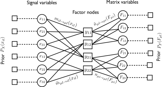
Figure 1: Factor graph used for the belief propagation inference, here drawn using $N=3$, $P=2$ and $M=2$. The factor nodes are associated to the probability $P_{\rm out}(y_{\mu l\!}|\!\sum_{i}F_{\mu i}X_{il})$.

The factor graph corresponding to the posterior probability (5) is depicted in Fig. 1. The canonical BP iterative equations Kschischang et al. (2001) are written using messages $m_{il\to\mu l}(X_{il})$, $n_{\mu i\to\mu l}(F_{\mu i})$ from variables to factors, and using messages ${\tilde{m}}_{\mu l\to il}(X_{il})$, ${\tilde{n}}_{\mu l\to\mu i}(F_{\mu i})$ from factors to variables. On tree graphical models the messages are defined as marginal probabilities of their arguments conditioned to the fact that the variable/factor to which the message is incoming is not present in the graph. The following BP equations provide the exact values for these conditional marginals on trees

$$m_{il\to\mu l}(t+1,X_{il}) = \frac{1}{{\cal Z}_{il\to\mu l}}P_{X}(X_{il})\prod_{\nu(\neq\mu)}^{M}\tilde{m}_{\nu l\to il}(t,X_{il})\,,$$ (41)

$$n_{\mu i\to\mu l}(t+1,F_{\mu i}) = \frac{1}{{\cal Z}_{\mu i\to\mu l}}P_{F}(F_{\mu i})\prod_{n(\neq l)}^{P}\tilde{n}_{\mu n\to\mu i}(t,F_{\mu i})\,,$$ (42)

$$\tilde{m}_{\mu l\to il}(t,X_{il}) = \frac{1}{{\cal Z}_{\mu l\to il}}\int\prod_{j(\neq i)}^{N}{\rm d}X_{jl}\prod_{k}^{N}dF_{\mu k}\,P_{\rm out}(y_{\mu l}|\sum_{k}^{N}F_{\mu k}X_{kl})\prod_{k}^{N}n_{\mu k\to\mu l}(t,F_{\mu k})\prod_{j(\neq i)}^{N}m_{jl\to\mu l}(t,X_{jl})\,,$$ (43)

$$\tilde{n}_{\mu l\to\mu i}(t,F_{\mu i}) = \frac{1}{{\cal Z}_{\mu l\to\mu i}}\int\prod_{j}^{N}{\rm d}X_{jl}\prod_{k(\neq i)}^{N}dF_{\mu k}\,P_{\rm out}(y_{\mu l}|\sum_{k}^{N}F_{\mu k}X_{kl})\prod_{k(\neq i)}^{N}n_{\mu k\to\mu l}(t,F_{\mu k})\prod_{j}^{N}m_{jl\to\mu l}(t,X_{jl})\,,$$ (44)

where ${\cal Z}_{il\to\mu l}$, ${\cal Z}_{\mu i\to\mu l}$, ${\cal Z}_{\mu l\to il}$, ${\cal Z}_{\mu l\to\mu i}$ are normalization constants ensuring that all the messages are probability distributions, $t\in{\mathbb{N}}$ is denoting the iteration time-step, and the notation $\prod_{\nu(\neq\mu)}^{M}$ means a product over all integer values of $\nu$ in $\{1,\dots,M\}$, except the value $\mu$.

Of course, the factor graph of matrix factorization, shown in Fig. 1, is extremely far from a tree. The above BP equations can, however, still be asymptotically exact if the dependence between the incoming messages is negligible in the leading order in $N$. This indeed happens in compressed sensing (where the matrix $F$ is a known matrix, generated randomly with zero mean), as follows from the rigorously proven success of approximate message passing Donoho et al. (2009); Bayati & Montanari (2011). In the present case of matrix factorization, we do not have any rigorous proof yet, but based on our experience from studies of mean field spin glass systems Mézard et al. (1987); Mézard & Montanari (2009), we conjecture that the fixed points of the above belief propagation equations describe asymptotically exactly (in the same sense as for compressed sensing) the performance of Bayes-optimal inference. Hence the analysis of the fixed points of the above equations leads to the understanding of information-theoretic limitations for matrix factorization. The associated phase transitions describe possible algorithmic barriers. This analysis is the main goal and result of the present paper.

The above BP iterative equations are written for probability distributions over real values variables and the $2N-1$-uple integrals from the r.h.s. are mathematically intractable in this form. We now define means and variances of the variable-to-factor messages as

$${\hat{x}}_{il\to\mu l}(t) = \int{\rm d}X_{il}\,m_{il\to\mu l}(t,X_{il})\,X_{il}\,,$$ (45)

$$c_{il\to\mu l}(t)+{\hat{x}}^{2}_{il\to\mu l}(t) = \int{\rm d}X_{il}\,m_{il\to\mu l}(t,X_{il})\,X^{2}_{il}\,,$$ (46)

$${\hat{f}}_{\mu i\to\mu l}(t) = \sqrt{N}\int{\rm d}F_{\mu i}\,n_{\mu i\to\mu l}(t,F_{\mu i})\,F_{\mu i}\,,$$ (47)

$$s_{\mu i\to\mu l}(t)+{\hat{f}}^{2}_{\mu i\to\mu l}(t) = N\int{\rm d}F_{il}\,n_{\mu i\to\mu l}(t,F_{\mu i})\,F^{2}_{\mu i}\,.$$ (48)

Notice that the factors $\sqrt{N}$ in the definition of $r$, and $N$ in the definition of $s$, have been introduced in order to ensure that all the messages $a,c,r,s$ are of order $O(1)$ in the thermodynamic limit.

Using this scaling, we shall now show that the BP equations can be simplified in the thermodynamic limit, and that they can actually be written as a closed set of equations involving only messages $a,c,r,s$. Our general aim is to design an algorithm which in some region of parameters will asymptotically match the performance of the exact (computationally intractable) Bayes-optimal inference. Belief propagation provides such an algorithm, but in order to make it computationally efficient, writing it in terms of the messages $a,c,r,s$ is crucial, provided one is careful not to loose any terms in the asymptotic analysis of the thermodynamic limit to leading order.

Let us define the Fourrier transform of the output function

$$\hat{P}_{\rm out}(y,\xi)=\frac{1}{\sqrt{2\pi}}\int_{-\infty}^{\infty}P_{\rm out}(y|z)e^{-i\xi z}{\rm d}z\,,$$ (49)

to rewrite the update equation for message $\tilde{m}_{\mu l\to il}(t,X_{il})$ as

$$\tilde{m}_{\mu l\to il}(t,X_{il}) = \frac{1}{\sqrt{2\pi}{\cal Z}_{\mu l\to il}}\int{\rm d}\xi\,\hat{P}_{\rm out}(y_{\mu l},\xi)\int{\rm d}F_{\mu i}\,e^{i\xi F_{\mu i}X_{il}}n_{\mu i\to\mu l}(t,F_{\mu i})$$ (50)

$$\prod_{j(\neq i)}^{N}\left[\int{\rm d}X_{jl}{\rm d}F_{\mu j}\,e^{i\xi F_{\mu j}X_{jl}}n_{\mu j\to\mu l}(t,F_{\mu j})m_{jl\to\mu l}(t,X_{jl})\right]\,.$$

In order to perform the integral in the square-bracket we recall that the elements of matrix $F=O(1/\sqrt{N})$ and hence we can expand the exponential to second order, use definitions (80-83) and re-exponentiate the result without loosing any leading order terms in $\tilde{m}_{\mu l\to il}(t,X_{il})$. The whole square bracket then becomes

$$\exp\left\{i\frac{\xi}{\sqrt{N}}{\hat{f}}_{\mu j\to\mu l}(t){\hat{x}}_{jl\to\mu l}(t)-\frac{\xi^{2}}{2N}\left[s_{\mu j\to\mu l}(t)c_{jl\to\mu l}(t)+s_{\mu j\to\mu l}(t){\hat{x}}^{2}_{jl\to\mu l}(t)+{\hat{f}}^{2}_{\mu j\to\mu l}(t)c_{jl\to\mu l}(t)\right]\right\}\,.$$ (51)

Next we perform the integral over variable $\xi$ which is simply a Gaussian integral. This gives for the message

$$\tilde{m}_{\mu l\to il}(t,X_{il})=\frac{1}{{\cal Z}_{\mu l\to il}}\int{\rm d}F_{\mu i}\,n_{\mu i\to\mu l}(t,F_{\mu i})\frac{1}{\sqrt{2\pi V^{t}_{\mu il}}}\int{\rm d}z\,P_{\rm out}(y_{\mu l}|z)e^{-\frac{(z-F_{\mu i}X_{il}-\omega^{t}_{\mu il})^{2}}{2V^{t}_{\mu il}}}\,,$$ (52)

where we introduced auxiliary variables that are both of order $O(1)$

$$V^{t}_{\mu il} \equiv \frac{1}{N}\sum_{j(\neq i)}^{N}\left[s_{\mu j\to\mu l}(t)c_{jl\to\mu l}(t)+s_{\mu j\to\mu l}(t){\hat{x}}^{2}_{jl\to\mu l}(t)+{\hat{f}}^{2}_{\mu j\to\mu l}(t)c_{jl\to\mu l}(t)\right]\,,$$ (53)

$$\omega^{t}_{\mu il} \equiv \frac{1}{\sqrt{N}}\sum_{j(\neq i)}^{N}{\hat{f}}_{\mu j\to\mu l}(t){\hat{x}}_{jl\to\mu l}(t)\,.$$ (54)

The last integral to be performed in (52) is the one over the matrix element $F_{\mu i}$. Using again the fact that $F_{\mu i}=O(1/\sqrt{N})$, we expand the exponential in which $F_{\mu i}$ appears to second order and perform the integration to obtain

$$\tilde{m}_{\mu l\to il}(t,X_{il}) = \frac{1}{{\cal Z}_{\mu l\to il}}\frac{1}{\sqrt{2\pi V^{t}_{\mu il}}}\int{\rm d}z\,P_{\rm out}(y_{\mu l}|z)e^{-\frac{(z-\omega^{t}_{\mu il})^{2}}{2V^{t}_{\mu il}}}$$ (55)

$$\left\{1+\frac{z-\omega^{t}_{\mu il}}{\sqrt{N}V^{t}_{\mu il}}{\hat{f}}_{\mu i\to\mu l}(t)X_{il}-\frac{X_{il}^{2}}{2N}\left[\frac{1}{V^{t}_{\mu il}}-\frac{(z-\omega^{t}_{\mu il})^{2}}{(V^{t}_{\mu il})^{2}}\right]\left[{\hat{f}}^{2}_{\mu i\to\mu l}(t)+s_{\mu i\to\mu l}(t)\right]\right\}\,.$$

Following the notation of Rangan (2011) we now define the output-function as

$$g_{\rm out}(\omega,y,V)\equiv\frac{\int{\rm d}zP_{\rm out}(y|z)\,(z-\omega)\,e^{-\frac{(z-\omega)^{2}}{2V}}}{V\int{\rm d}zP_{\rm out}(y|z)e^{-\frac{(z-\omega)^{2}}{2V}}}\,.$$ (56)

The following useful identity holds for the average of $(z-\omega)^{2}/V^{2}$ in the above measure

$$\frac{\int{\rm d}zP_{\rm out}(y|z)\,(z-\omega)^{2}\,e^{-\frac{(z-\omega)^{2}}{2V}}}{V^{2}\int{\rm d}zP_{\rm out}(y|z)e^{-\frac{(z-\omega)^{2}}{2V}}}=\frac{1}{V}+\partial_{\omega}g_{\rm out}(\omega,y,V)+g^{2}_{\rm out}(\omega,y,V)\,.$$ (57)

With definition (56), and re-exponentiating the $X_{il}$-dependent terms in (55) while keeping all the leading order terms, we obtain finally that $\tilde{m}_{\mu l\to il}(t,X_{il})$ is a Gaussian probability distribution

$$\tilde{m}_{\mu l\to il}(t,X_{il})=\sqrt{\frac{A^{t}_{\mu l\to il}}{2\pi N}}e^{-\frac{X_{il}^{2}}{2N}A^{t}_{\mu l\to il}+B^{t}_{\mu l\to il}\frac{X_{il}}{\sqrt{N}}-\frac{(B^{t}_{\mu l\to il})^{2}}{2A^{t}_{\mu l\to il}}}\\$$ (58)

with

$$B^{t}_{\mu l\to il} = g_{\rm out}(\omega^{t}_{\mu il},y_{\mu l},V^{t}_{\mu il})\,{\hat{f}}_{\mu i\to\mu l}(t)\,,$$ (59)

$$A^{t}_{\mu l\to il} = -\partial_{\omega}g_{\rm out}(\omega^{t}_{\mu il},y_{\mu l},V^{t}_{\mu il})\,\left[{\hat{f}}^{2}_{\mu i\to\mu l}(t)+s_{\mu i\to\mu l}(t)\right]-g^{2}_{\rm out}(\omega^{t}_{\mu il},y_{\mu l},V^{t}_{\mu il})\,s_{\mu i\to\mu l}(t)\,.$$ (60)

In a completely analogous way we obtain that the message $\tilde{n}_{\mu l\to\mu i}(t,F_{\mu i})$ is also a Gaussian distribution

$$\tilde{n}_{\mu l\to\mu i}(t,F_{\mu i})=\sqrt{\frac{S^{t}_{\mu l\to\mu i}}{2\pi}}e^{-\frac{F_{\mu i}^{2}}{2}S^{t}_{\mu l\to\mu i}+R^{t}_{\mu l\to\mu i}F_{\mu i}-\frac{(R^{t}_{\mu l\to\mu i})^{2}}{2S^{t}_{\mu l\to\mu i}}}$$ (61)

with

$$R^{t}_{\mu l\to\mu i} = g_{\rm out}(\omega^{t}_{\mu il},y_{\mu l},V^{t}_{\mu il})\,{\hat{x}}_{il\to\mu l}(t)\,,$$ (62)

$$S^{t}_{\mu l\to\mu i} = -\partial_{\omega}g_{\rm out}(\omega^{t}_{\mu il},y_{\mu l},V^{t}_{\mu il})\,\left[c_{il\to\mu l}(t)+{\hat{x}}^{2}_{il\to\mu l}(t)\right]-g^{2}_{\rm out}(\omega^{t}_{\mu il},y_{\mu l},V^{t}_{\mu il})\,c_{il\to\mu l}(t)\,.$$ (63)

At this point we follow closely the derivation of AMP from Krzakala et al. (2012) and define the probability distributions

$${\cal M}_{X}(\Sigma,T,X)=\frac{1}{\hat{Z}_{X}(\Sigma,T)}P_{X}(X)\frac{1}{\sqrt{2\pi\Sigma}}e^{-\frac{(X-T)^{2}}{2\Sigma}}\,,$$ (64)

$${\cal M}_{F}(Z,W,F)=\frac{1}{\hat{Z}_{F}(Z,W)}P_{F}(F)\frac{1}{\sqrt{2\pi Z}}e^{-\frac{(\sqrt{N}F-W)^{2}}{2Z}}\,,$$ (65)

where $\hat{Z}_{X}(\Sigma,T)$, and $\hat{Z}_{F}(Z,W)$ are normalizations. We define the average and variance of ${\cal M}_{X}$ and ${\cal M}_{F}$ as

$$f_{X}(\Sigma,T) \equiv \int{\rm d}X\,X\,{\cal M}_{X}(\Sigma,T,X)\,,\quad\quad f_{c}(\Sigma,T)\equiv\int{\rm d}X\,X^{2}\,{\cal M}_{X}(\Sigma,T,X)-f^{2}_{a}(\Sigma,T)\,,$$ (66)

$$f_{F}(Z,W) \equiv \sqrt{N}\int{\rm d}F\,F\,{\cal M}_{F}(Z,W,F)\,,\quad\quad f_{s}(Z,W)\equiv N\int{\rm d}F\,F^{2}\,{\cal M}_{F}(Z,W,F)-f^{2}_{r}(Z,W)\,.$$ (67)

These are the input auxiliary function of Rangan (2011). It is instrumental to notice that

$$f_{X}(\Sigma,T)=T+\Sigma\frac{{\rm d}}{{\rm d}T}\log{\hat{Z}_{X}(\Sigma,T)}\,,\quad\quad f_{c}(\Sigma,T)=\Sigma\frac{{\rm d}}{{\rm d}T}f_{X}(\Sigma,T)\,.$$ (68)

and analogously for $f_{F}$ and $f_{s}$

$$f_{F}(Z,W)=W+Z\frac{{\rm d}}{{\rm d}W}\log{\hat{Z}_{F}(Z,W)}\,,\quad\quad f_{s}(Z,W)=Z\frac{{\rm d}}{{\rm d}W}f_{F}(Z,W)\,.$$ (69)

With these definition we obtain from (41,42) using (58,61) that

$${\hat{x}}_{il\to\mu l}(t+1) = f_{X}\left(\frac{N}{\sum_{\nu(\neq\mu)}A^{t}_{\nu l\to il}},\frac{\sqrt{N}\sum_{\nu(\neq\mu)}B^{t}_{\nu l\to il}}{\sum_{\nu(\neq\mu)}A^{t}_{\nu l\to il}}\right)\,,$$ (70)

$$c_{il\to\mu l}(t+1) = f_{c}\left(\frac{N}{\sum_{\nu(\neq\mu)}A^{t}_{\nu l\to il}},\frac{\sqrt{N}\sum_{\nu(\neq\mu)}B^{t}_{\nu l\to il}}{\sum_{\nu(\neq\mu)}A^{t}_{\nu l\to il}}\right)\,,$$ (71)

$${\hat{f}}_{\mu i\to\mu l}(t+1) = f_{F}\left(\frac{N}{(\sum_{n(\neq l)}S^{t}_{\mu n\to\mu i}},\frac{\sqrt{N}\sum_{n(\neq l)}R^{t}_{\mu n\to\mu i}}{\sum_{n(\neq l)}S^{t}_{\mu n\to\mu i}}\right)\,,$$ (72)

$$s_{\mu i\to\mu l}(t+1) = f_{s}\left(\frac{N}{\sum_{n(\neq l)}S^{t}_{\mu n\to\mu i}},\frac{\sqrt{N}\sum_{n(\neq l)}R^{t}_{\mu n\to\mu i}}{\sum_{n(\neq l)}S^{t}_{\mu n\to\mu i}}\right)\,,$$ (73)

It is clear from the above expressions that all the messages $a,c,r,s$ and $A,C,R,S$ scale as $O(1)$ in the thermodynamic limit. For instance, as $A$ are positive, the quantity $\sum_{\nu(\neq\mu)}A^{t}_{\nu l\to il}$ is $O(1)$. On the other hand, the message ${\hat{f}}_{\mu i\to\mu l}(t)$ is an estimate of $\sqrt{N}F_{\mu i}$; this estimate is $O(1)$, but a sum like $(1/\sqrt{N})\sum_{\nu(\neq\mu)}{\hat{f}}_{\nu i\to\nu l}(t)$ is an estimate of $\sum_{\nu}F_{\nu i}$. As $P_{F}$ has mean variance of order $O(1/N)$, this sum is actually of $O(1)$. The same argument suggests that $(1/\sqrt{N})\sum_{\nu(\neq\mu)}B^{t}_{\nu l\to il}$ is $O(1)$. Recalling eqs. (59,60) and (62,63), we have derived that in the thermodynamic limit the general belief propagation equations simplify into a closed set of equations in the messages which are the means and variances $a,r,c,s$ defined in (45-48). To iterate this message passing algorithm we initialize as

$${\hat{x}}_{il\to\mu l}(0) = \int{\rm d}X\,XP^{il}_{X}(X)\,,$$ (74)

$$c_{il\to\mu l}(0) = \int{\rm d}X\,X^{2}P^{il}_{X}(X)-{\hat{x}}^{2}_{il\to\mu l}(0)\,,$$ (75)

$${\hat{f}}_{\mu i\to\mu l}(0) = \sqrt{N}\int{\rm d}F\,FP^{\mu l}_{F}(F)\,,$$ (76)

$$s_{\mu i\to\mu l}(0) = N\int{\rm d}F\,F^{2}P^{\mu l}_{F}(F)-{\hat{f}}^{2}_{\mu i\to\mu l}(0)\,,$$ (77)

then we compute $V^{t}_{\mu il}$ and $\omega^{t}_{\mu il}$ from (53-54), then we compute $B^{t}$, $A^{t}$, $R^{t}$ and $S^{t}$ according to (59-60) and (62-63) using definition of $g_{\rm out}$ (56). Finally we update the messages according to (70-73) and iterate. Notice, however, that we work with $O(N^{3})$ messages, each of them takes $N$ steps to update, and hence the computational complexity of this algorithm is relatively high. In the next section we will write a simplification that reduces this complexity.

From the fixed point of the belief propagation equations one can also compute the approximated marginal probabilities of the posterior, defined as

$$m_{il}(t+1,X_{il}) = \frac{1}{{\cal Z}_{il}}P_{X}(X_{il})\prod_{\nu}^{M}\tilde{m}_{\nu l\to il}(t,X_{il})\,,$$ (78)

$$n_{\mu i}(t+1,F_{\mu i}) = \frac{1}{{\cal Z}_{\mu i}}P_{F}(F_{\mu i})\prod_{n}^{P}\tilde{n}_{\mu n\to\mu i}(t,F_{\mu i})\,,$$ (79)

One again defines the mean and variance of these two messages, ${\hat{x}}_{il}(t+1)$, $c_{il}(t+1)$, ${\hat{f}}_{\mu i}(t+1)$ and $s_{\mu i}(t+1)$ analogously to (80-83):

$${\hat{x}}_{il}(t+1) = \int{\rm d}X_{il}\,m_{il}(t+1,X_{il})\,X_{il}\,,$$ (80)

$$c_{il}(t+1)+{\hat{x}}^{2}_{il}(t+1) = \int{\rm d}X_{il}\,m_{il}(t+1,X_{il})\,X^{2}_{il}\,,$$ (81)

$${\hat{f}}_{\mu i}(t+1) = \sqrt{N}\int{\rm d}F_{\mu i}\,n_{\mu i}(t+1,F_{\mu i})\,F_{\mu i}\,,$$ (82)

$$s_{\mu i}(t+1)+{\hat{f}}^{2}_{\mu i}(t+1) = N\int{\rm d}F_{il}\,n_{\mu i}(t+1,F_{\mu i})\,F^{2}_{\mu i}\,.$$ (83)

Those quantities are then expressed as

$${\hat{x}}_{il}(t+1) = f_{X}\left(\frac{N}{\sum_{\nu}A^{t}_{\nu l\to il}},\frac{\sqrt{N}\sum_{\nu}B^{t}_{\nu l\to il}}{\sum_{\nu}A^{t}_{\nu l\to il}}\right)\,,$$ (84)

$$c_{il}(t+1) = f_{c}\left(\frac{N}{\sum_{\nu}A^{t}_{\nu l\to il}},\frac{\sqrt{N}\sum_{\nu}B^{t}_{\nu l\to il}}{\sum_{\nu}A^{t}_{\nu l\to il}}\right)\,,$$ (85)

$${\hat{f}}_{\mu i}(t+1) = f_{F}\left(\frac{N}{\sum_{n}S^{t}_{\mu n\to\mu i}},\frac{\sqrt{N}\sum_{n}R^{t}_{\mu n\to\mu i}}{\sum_{n}S^{t}_{\mu n\to\mu i}}\right)\,,$$ (86)

$$s_{\mu i}(t+1) = f_{s}\left(\frac{N}{\sum_{n}S^{t}_{\mu n\to\mu i}},\frac{\sqrt{N}\sum_{n}R^{t}_{\mu n\to\mu i}}{\sum_{n}S^{t}_{\mu n\to\mu i}}\right)\,.$$ (87)

III.2 GAMP for matrix factorization

The message-passing form the AMP algorithm for matrix factorization derived in the previous section uses $2NMP$ messages, one between each variable component $(il)$ and $(\mu i)$ and each measurement $(\mu l)$, in each iteration. In fact, exploiting again the simplifications which take place in the thermodynamic limit, always within the assumption that the elements of the matrix $F$ scale as $O(1/\sqrt{N})$, it is possible to rewrite and close the BP equations in terms of only $2N(P+M)$ messages. In statistical physics terms, the resulting equations correspond to the Thouless-Anderson-Palmer equations (TAP) Thouless et al. (1977) used in the study of spin glasses. In the thermodynamic limit, these are asymptotically equivalent to the BP equations. Going from BP to TAP is, in the compressed sensing literature, the step to go from the rBP Rangan (2010) to the AMP Donoho et al. (2009) algorithm. Let us now show how to take this step for the present problem of matrix factorization.

In the thermodynamic limit, it is clear from (70-73) that the messages ${\hat{x}}_{il\to\mu l}$, $v_{il\to\mu l}$ and ${\hat{f}}_{\mu i\to\mu l}$, $s_{\mu i\to\mu l}$ are nearly independent of $\mu l$. For instance in the equation giving ${\hat{x}}_{il\to\mu l}$, the only dependence on $\mu$ is through the fact that the sum over $\nu$ avoids the value $\nu=\mu$. But this is one term in $M$, and therefore one might expect that this term is negligible. However, one must be careful when these small terms are summed over and their sum might be of the leading order in $N$. Such terms are called in spin-glass theory the “Onsager reaction terms”. In the following we derive these Onsager terms.

Let us define the following variables all of order $O(1)$ on which we will close the equations

$$T^{t}_{il} = \frac{\sqrt{N}\sum_{\nu}B^{t}_{\nu l\to il}}{\sum_{\nu}A^{t}_{\nu l\to il}}\,,\quad\quad\Sigma^{t}_{il}=\frac{N}{\sum_{\nu}A^{t}_{\nu l\to il}}\,,$$ (88)

$$W^{t}_{\mu i} = \frac{\sqrt{N}\sum_{n}R^{t}_{\mu n\to\mu i}}{\sum_{n}S^{t}_{\mu n\to\mu i}}\,,\quad\quad Z^{t}_{\mu i}=\frac{N}{\sum_{n}S^{t}_{\mu n\to\mu i}}\,,$$ (89)

$$V^{t}_{\mu l} = \frac{1}{N}\sum_{j}[c_{jl\to\mu l}(t)s_{\mu j\to\mu l}(t)+c_{jl\to\mu l}(t){\hat{f}}^{2}_{\mu j\to\mu l}(t)+{\hat{x}}^{2}_{jl\to\mu l}(t)s_{\mu j\to\mu l}(t)]\,,$$ (90)

$$\omega^{t}_{\mu l} = \frac{1}{\sqrt{N}}\sum_{j}{\hat{x}}_{jl\to\mu l}(t){\hat{f}}_{\mu j\to\mu l}(t)\,.$$ (91)

To keep track of all the Onsager terms that will influence the leading order of the final equations we notice that

$${\hat{x}}_{il\to\mu l}(t+1) = f_{X}\left(\frac{N}{\sum_{\nu}A^{t}_{\nu l\to il}-A^{t}_{\mu l\to il}},\frac{\sqrt{N}\sum_{\nu}B^{t}_{\nu l\to il}-\sqrt{N}B^{t}_{\mu l\to il}}{\sum_{\nu}A^{t}_{\nu l\to il}-A^{t}_{\mu l\to il}}\right)\,,$$ (92)

$$= {\hat{x}}_{il}(t+1)-\frac{1}{\sqrt{N}}B^{t}_{\mu l\to il}\Sigma^{t}_{il}\frac{\partial f_{X}}{\partial T}\left(\Sigma^{t}_{il},T^{t}_{il}\right)+O\left(1/N\right)\,,$$

$$= {\hat{x}}_{il}(t+1)-\frac{1}{\sqrt{N}}g_{\rm out}(\omega^{t}_{\mu l},y_{\mu l},V^{t}_{\mu l}){\hat{f}}_{\mu i}(t)c_{il}(t+1)+O\left(1/N\right)\,.$$

Similarly:

$${\hat{f}}_{\mu i\to\mu l}(t+1) = {\hat{f}}_{\mu i}(t+1)-\frac{1}{\sqrt{N}}g_{\rm out}(\omega^{t}_{\mu l},y_{\mu l},V^{t}_{\mu l}){\hat{x}}_{il}(t)s_{\mu i}(t+1)+O\left(1/N\right)\,,$$ (93)

$$c_{il\to\mu l}(t+1) = c_{il}(t+1)+O\left(1/\sqrt{N}\right)\,,\quad\quad s_{\mu i\to\mu l}(t+1)=s_{\mu i}(t+1)+O\left(1/\sqrt{N}\right)\,,$$ (94)

$$g_{\rm out}(\omega^{t}_{\mu il},y_{\mu l},V^{t}_{\mu il}) = g_{\rm out}(\omega^{t}_{\mu l},y_{\mu l},V^{t}_{\mu l})-\frac{1}{\sqrt{N}}{\hat{f}}_{\mu i}(t){\hat{x}}_{il}(t)\partial_{\omega}g_{\rm out}(\omega^{t}_{\mu l},y_{\mu l},V^{t}_{\mu l})+O(1/N)\,,$$ (95)

From these expansions we obtain the GAMP algorithm for matrix factorization

$$V^{t}_{\mu l} = \frac{1}{N}\sum_{j}[c_{jl}(t)s_{\mu j}(t)+c_{jl}(t){\hat{f}}^{2}_{\mu j}(t)+{\hat{x}}^{2}_{jl}(t)s_{\mu j}(t)]\,,$$ (96)

$$\omega^{t}_{\mu l} = \frac{1}{\sqrt{N}}\sum_{j}{\hat{x}}_{jl}(t){\hat{f}}_{\mu j}(t)-g_{\rm out}(\omega^{t-1}_{\mu l},y_{\mu l},V^{t-1}_{\mu l})\frac{1}{N}\sum_{j}\left[{\hat{f}}_{\mu j}(t){\hat{f}}_{\mu j}(t-1)c_{jl}(t)+{\hat{x}}_{jl}(t){\hat{x}}_{jl}(t-1)s_{\mu j}(t)\right]\,,$$ (97)

$$(\Sigma^{t}_{il})^{-1} = \frac{1}{N}\sum_{\mu}\left\{-\partial_{\omega}g_{\rm out}(\omega^{t}_{\mu l},y_{\mu l},V^{t}_{\mu l})\,\left[{\hat{f}}^{2}_{\mu i}(t)+s_{\mu i}(t)\right]-g^{2}_{\rm out}(\omega^{t}_{\mu l},y_{\mu l},V^{t}_{\mu l})\,s_{\mu i}(t)\right\}\,,$$ (98)

$$T^{t}_{il} = \Sigma^{t}_{il}\Big{\{}\frac{1}{\sqrt{N}}\sum_{\mu}g_{\rm out}(\omega^{t}_{\mu l},y_{\mu l},V^{t}_{\mu l})\,{\hat{f}}_{\mu i}(t)-{\hat{x}}_{il}(t)\frac{1}{N}\sum_{\mu}{\hat{f}}^{2}_{\mu i}(t)\partial_{\omega}g_{\rm out}(\omega^{t}_{\mu l},y_{\mu l},V^{t}_{\mu l})$$ (99)

$$-{\hat{x}}_{il}(t-1)\frac{1}{N}\sum_{\mu}s_{\mu i}(t)g_{\rm out}(\omega^{t}_{\mu l},y_{\mu l},V^{t}_{\mu l})g_{\rm out}(\omega^{t-1}_{\mu l},y_{\mu l},V^{t-1}_{\mu l})\Big{\}}\,,$$

$$(Z^{t}_{\mu i})^{-1} = \frac{1}{N}\sum_{l}\left\{-\partial_{\omega}g_{\rm out}(\omega^{t}_{\mu l},y_{\mu l},V^{t}_{\mu l})\,\left[{\hat{x}}^{2}_{il}(t)+c_{il}(t)\right]-g^{2}_{\rm out}(\omega^{t}_{\mu l},y_{\mu l},V^{t}_{\mu l})\,c_{il}(t)\right\}\,,$$ (100)

$$W^{t}_{\mu i} = Z^{t}_{il}\Big{\{}\frac{1}{\sqrt{N}}\sum_{l}g_{\rm out}(\omega^{t}_{\mu l},y_{\mu l},V^{t}_{\mu l})\,{\hat{x}}_{il}(t)-{\hat{f}}_{\mu i}(t)\frac{1}{N}\sum_{l}{\hat{x}}^{2}_{il}(t)\partial_{\omega}g_{\rm out}(\omega^{t}_{\mu l},y_{\mu l},V^{t}_{\mu l})$$ (101)

$$-{\hat{f}}_{\mu i}(t-1)\frac{1}{N}\sum_{l}c_{il}(t)g_{\rm out}(\omega^{t}_{\mu l},y_{\mu l},V^{t}_{\mu l})g_{\rm out}(\omega^{t-1}_{\mu l},y_{\mu l},V^{t-1}_{\mu l})\Big{\}}\,,$$

$${\hat{x}}_{il}(t+1) = f_{X}(\Sigma^{t}_{il},T^{t}_{il})\,,\quad\quad c_{il}(t+1)=f_{c}(\Sigma^{t}_{il},T^{t}_{il})\,,$$ (102)

$${\hat{f}}_{\mu i}(t+1) = f_{F}(Z^{t}_{\mu i},W^{t}_{\mu i})\,,\quad\quad s_{\mu i}(t+1)=f_{s}(Z^{t}_{\mu i},W^{t}_{i\mu})\,.$$ (103)

The initial condition for iterations are

$${\hat{x}}_{il}(t=0) = \int{\rm d}X\,XP^{il}_{X}(X)\,,\quad\quad c_{il}(t=0)=\int{\rm d}X\,X^{2}P^{il}_{X}(X)-{\hat{x}}^{2}_{il\to\mu l}(t=0)\,,$$ (104)

$${\hat{f}}_{\mu i}(t=0) = \sqrt{N}\int{\rm d}F\,FP^{\mu i}_{F}(F)\,,\quad\quad s_{\mu i}(t=0)=N\int{\rm d}F\,F^{2}P^{\mu i}_{F}(F)-{\hat{f}}^{2}_{\mu i}(t=0)\,.$$ (105)

In order to compute $\omega^{t=0}$, $T^{t=0}$ and $W^{t=0}$ use the above equations as if ${\hat{f}}_{\mu i}(-1)=0$ and ${\hat{x}}_{il}(-1)=0$.

The interpretation of the terms in the GAMP for matrix factorization is the following: $\omega_{\mu l}^{t}$ is the mean of the current estimate of $z_{\mu l}=\sum_{i}F_{\mu i}X_{il}$ and $V^{t}_{\mu l}$ is the variance of that estimate; $T_{il}$ and $\Sigma_{il}$ is the mean and variance of the current estimate of $X_{il}$ without taking into account the prior information of $X_{il}$; the parameters ${\hat{x}}_{il}$ and $c_{il}$ are then the mean and variance of the current estimate of $X_{il}$ with the prior information taken into account. Analogously for $W_{\mu i}$ and $Z_{\mu i}$ being the mean and variance of the estimate for $F_{\mu i}$ before the prior is taken into account, and ${\hat{f}}_{\mu i}$ with $s_{\mu i}$ are the mean and variance once the prior information was accounted for.

A reader familiar with the AMP and GAMP algorithm for compressed sensing Donoho et al. (2009); Rangan (2011); Krzakala et al. (2012) will recognize that the above equations indeed reduce to the compressed sensing GAMP of Rangan (2011) when one sets ${\hat{f}}_{\mu i}(t)=\sqrt{N}F_{\mu i}$ and $s_{\mu i}=0$.

The above algorithm is closely related to the BiG-AMP of Parker et al. (2013). There are however three differences between our algorithm and BiG-AMP:

1. We find a $s_{\mu i}$-dependent term in the expression (98) for $\Sigma_{il}$ which is not present in BiG-AMP.

2. Similarly, we find a $c_{il}$-dependent term in the expression (100) for $Z_{\mu i}$ which is not present in BiG-AMP.

3. The time indices are slightly different.

Considering the last point, the fact of having different time indices during the iterations does not influence the fixed points, in which we are mainly interested. However, the use of correct time indices is crucial for the assumptions leading to the density evolution of this algorithm (that we derive in section V.1) to hold.

As for the missing terms in the BiG-AMP expressions of Parker et al. (2013) for $\Sigma_{il}$ and $Z_{\mu i}$, they have a more serious effect as they can change the fixed point. To the best of our understanding, these terms have been neglected in Parker et al. (2013), while they should be kept. It seems to us that some of the leading order terms are missing in eqs. (15-16) from Parker et al. (2013).

III.3 Simplifications due to the Nishimori identities

In the previous section we derived the GAMP algorithm for matrix factorization, eqs. (96-103). This algorithm can in principle be used for any set of matrices $F$ and $X$. If iterated in the form derived in Section III.2 it often shows problems of convergence. There are ways to slightly improve the convergence of the above algorithm in a wide range of applications by a number of empirical methods suggested in Parker et al. (2014).

We will focus on the particular case when matrices $X$ and $F$ were indeed generated from the separable probability distributions $P_{F}(F)$ and $P_{X}(X)$ described in eqs. (3-4), and the output $y$ was generated by the assumed model.

$$P_{X}(X)=P_{X^{0}}(X)\,,\quad\quad P_{F}(F)=P_{F^{0}}(F)\,,\quad\quad P^{0}_{\rm out}(y|z)=P_{\rm out}(y|z)\,.$$ (106)

In this case the belief propagation is a proxy for the optimal Bayes inference algorithms and a number of properties described in section I.2 hold. In analogy with fundamental works on spin glasses Nishimori (2001); Iba (1999) we called these properties the Nishimori identities. The setting where conditions (106) hold will be called the Bayes-optimal setting.

The Nishimori identities hold and the system is on the Nishimori line when one is using the correct priors on $F$ and $X$ and the right output channel in the reconstruction process, i.e. when conditions (106) hold. In the limit $N\to\infty$ and thanks to self-averaging we then have on the Nishimori line at every iteration step $t$

$$\frac{1}{PM}\sum_{\mu,l}\frac{\int{\rm d}zP_{\rm out}(y_{\mu l}|z)(z-\omega_{\mu l}^{t})^{2}e^{-\frac{(z-\omega_{\mu l}^{t})^{2}}{2V_{\mu l}^{t}}}}{\int{\rm d}zP_{\rm out}(y_{\mu l}|z)e^{-\frac{(z-\omega_{\mu l}^{t})^{2}}{2V_{\mu l}^{t}}}}=\frac{1}{MP}\sum_{\mu,l}V_{\mu l}^{t}\,.$$ (107)

The meaning of this identity is that the mean squared error of the current estimate of $Z=FX$ computed from the current estimates of variances $V_{\mu l}^{t}$ is equal to the mean squared difference between the true $Z$ and its current estimate $\omega_{\mu l}^{t}$. Using the above expression and eq. (57) we obtain an identity

$$-\frac{1}{MP}\sum_{\mu,l}\partial_{\omega}g_{\rm out}(\omega_{\mu l}^{t},y_{\mu l},V^{t}_{\mu l})=\frac{1}{MP}\sum_{\mu,l}g^{2}_{\rm out}(\omega_{\mu l}^{t},y_{\mu l},V^{t}_{\mu l})\,.$$ (108)

The above identity holds also if the sum is only over $\mu$ or only over $l$. Finally using the conditional independence assumed in BP between the incoming messages we get also

$$-\frac{1}{M}\sum_{\mu}\partial_{\omega}g_{\rm out}(\omega_{\mu l}^{t},y_{\mu l},V^{t}_{\mu l})s_{\mu i}(t)=\frac{1}{M}\sum_{\mu}g^{2}_{\rm out}(\omega_{\mu l}^{t},y_{\mu l},V^{t}_{\mu l})s_{\mu i}(t)\,.$$ (109)

Under this condition we can simplify considerably the expressions for $\Sigma_{il}^{t}$ and $Z_{\mu i}^{t}$ and get

$$(\Sigma^{t}_{il})^{-1} = -\frac{1}{N}\sum_{\mu}\partial_{\omega}g_{\rm out}(\omega^{t}_{\mu l},y_{\mu l},V^{t}_{\mu l})\,{\hat{f}}^{2}_{\mu i}(t)\,,$$ (110)

$$(Z^{t}_{\mu i})^{-1} = -\frac{1}{N}\sum_{l}\partial_{\omega}g_{\rm out}(\omega^{t}_{\mu l},y_{\mu l},V^{t}_{\mu l})\,{\hat{x}}^{2}_{il}(t)\,.$$ (111)

Note that the r.h.s. of the two above equations is always strictly positive, which is reassuring given these expressions play the role of a variance of a probability distribution. Note also that the BiG-AMP algorithm of Parker et al. (2013) uses expressions (110,111) instead of (98,100), however, without mentioning the reason.

III.4 Simplification for matrices with random entries

Relying on the definitions of order parameters (161-162) and using part of the results on section V.1 we can write a version of the GAMP for matrix factorization that is in the leading order in $N$ equivalent to (96-103) for matrices $X$ and $F$ having iid elements.

Let us define the analog of $\hat{\chi}^{t}$ and $\hat{q}^{t}$ (168-169) as empirical means of the corresponding functions

$$\tilde{\chi}^{t} \equiv -\frac{1}{MP}\sum_{\mu,l}\partial_{\omega}g_{\rm out}(\omega_{\mu il}^{t},y_{\mu l},V^{t}_{\mu il})\,,$$ (112)

$$\tilde{q}^{t} \equiv \frac{1}{MP}\sum_{\mu,l}g^{2}_{\rm out}(\omega_{\mu il}^{t},y_{\mu l},V^{t}_{\mu il})\,.$$ (113)

Anticipating the reasoning that we shall use later in section V.1, we realize that in the leading order quantities $V^{t}_{il}$, $\Sigma^{t}_{il}$ and $Z^{t}_{\mu i}$ do not depend on their indices $i,l,\mu$. We have

$$V^{t} = Q^{t}_{F}Q^{t}_{X}-q^{t}_{F}q^{t}_{X}\,,$$ (114)

$$(\Sigma^{t})^{-1} = \alpha Q_{F}^{t}\tilde{\chi}^{t}-\alpha(Q_{F}^{t}-q_{F}^{t})\tilde{q}^{t}\,,$$ (115)

$$(Z^{t})^{-1} = \pi Q_{X}^{t}\tilde{\chi}^{t}-\pi(Q_{X}^{t}-q_{X}^{t})\tilde{q}^{t}\,.$$ (116)

where we define

$$q^{t}_{X} \equiv \frac{1}{NP}\sum_{jl}{\hat{x}}^{2}_{jl}(t)\,,\quad\quad q^{t}_{F}\equiv\frac{1}{NM}\sum_{\mu i}{\hat{f}}^{2}_{\mu i}(t)\,,$$ (117)

$$Q^{t}_{X} \equiv q^{t}_{X}+\frac{1}{NP}\sum_{jl}c_{jl}(t)\,,\quad\quad Q^{t}_{F}\equiv q^{t}_{F}+\frac{1}{NM}\sum_{\mu i}s_{\mu i}(t)\,.$$ (118)

These three equations can hence replace (96), (98) and (100) in GAMP. Furthermore, if we focus on the fixed point and hence disregard some of the time indices eqs. (97), (99) and (101) can be simplified as

$$\omega_{\mu l}^{t} = \frac{1}{\sqrt{N}}\sum_{j}{\hat{x}}_{jl}(t){\hat{f}}_{\mu j}(t)-g_{\rm out}(\omega_{\mu l}^{t-1},y_{\mu l},V^{t-1})(Q_{X}^{t}q_{F}^{t}+q_{F}^{t}Q_{X}^{t}-2q_{F}^{t}q_{X}^{t})\,,$$ (119)

$$T_{il}^{t} = \Sigma^{t}\left\{\frac{1}{\sqrt{N}}\sum_{\mu}g_{\rm out}(\omega_{\mu l}^{t},y_{\mu l},V^{t}){\hat{f}}_{\mu i}(t)+\alpha{\hat{x}}_{il}(t)\tilde{\chi}^{t}\,q_{F}^{t}-\alpha{\hat{x}}_{il}(t)(Q_{F}^{t}-q_{F}^{t})\tilde{q}^{t}\right\}\,,$$ (120)

$$W_{\mu i}^{t} = Z^{t}\left\{\frac{1}{\sqrt{N}}\sum_{l}g_{\rm out}(\omega_{\mu l}^{t},y_{\mu l},V^{t}){\hat{x}}_{il}(t)+\pi{\hat{f}}_{\mu i}(t)\tilde{\chi}^{t}\,q_{X}^{t}-\pi{\hat{f}}_{\mu i}(t)(Q_{X}^{t}-q_{X}^{t})\tilde{q}^{t}\right\}\,.$$ (121)

Within the Bayes-optimal setting of (106), we can use the Nishimori identity (108) to show that $\tilde{\chi}^{t}=\tilde{q}^{t}$. Consequently we can use only one of those parameters computed either from (112) or from (113). The equations then further simplify to strictly positive expressions for the variance-parameters

$$(\Sigma^{t})^{-1}=\alpha q_{F}^{t}\tilde{q}^{t}\,,\quad\quad(Z^{t})^{-1}=\pi q_{X}^{t}\tilde{q}^{t}\,.$$ (122)

The set of eqs. (102-103), (114), (119-122) was presented for the simple output channel with white noise in Krzakala et al. (2013). We detail this procedure for the generic output in Alg. 1.

Algorithm 1 Bayes-optimal Approximate Message Passing for Matrix Factorization

  Input: $\mathbf{y}$

  Initialize: $\mathbf{\hat{x}}$,$\mathbf{\hat{f}}$,$\mathbf{c}$,$\mathbf{s}$, ${\rm Iter}=1$

  Initialize: $\{\omega_{\mu l},V\}$

  repeat

     Compute averages, eqs. (117) and (118).

     AMP Update of $\{\omega_{\mu l},V\}$, eq. (119) and eq. (114).

     AMP Update of $\Sigma$ and $Z$, eq. (122).

     AMP Update of $\{T_{il}\}$,$\{W_{\mu i}\}$, eq. (120) and eq. (121).

     AMP Update of the estimed quantities $\mathbf{\hat{x}}$,$\mathbf{\hat{f}}$,$\mathbf{c}$,$\mathbf{s}$, eq. (102) and eq. (103).

     ${\rm Iter}\leftarrow{\rm Iter}+1$

  until Convergence on $\mathbf{\hat{x}}$,$\mathbf{\hat{f}}$

We want to stress here that all these simplifications take place for any output channel $P_{\rm out}(y|z)$. In contrast with the “uniform variance” approximation of Parker et al. (2013) the above result does not mean that the variances $c_{il}$ and $s_{\mu i}$ are independent in the leading order on their indices. On the contrary, these variances depend on their indices even in the simplest case of GAMP when the matrix $F_{\mu i}$ is known, i.e. for the compressed sensing problem.

IV The Bethe free entropy

The fixed point of the belief propagation equations or its AMP version can be used to estimate the posterior likelihood, i.e. the normalization ${\cal Z}(Y)$ of the posterior probability (5). The logarithm of this normalization is called the Bethe free entropy in statistical physics Yedidia et al. (2003). Negative logarithm of the normalization is called the free energy, in physics there is usually a temperature associated to the free energy. Bethe free entropy is computed from the fixed point of the BP equations (41-44) as Yedidia et al. (2003); Mézard & Montanari (2009):

$$\Phi^{\rm Bethe}=\sum_{\mu l}\log{{\cal Z}^{\mu l}}+\sum_{\mu i}\log{{\cal Z}^{\mu i}}+\sum_{il}\log{{\cal Z}^{il}}-\sum_{\mu il}\log{{\cal Z}^{il,\mu l}}-\sum_{\mu il}\log{{\cal Z}^{\mu i,\mu l}}\,,$$ (123)

where the five contributions are

$${\cal Z}^{\mu i} = \int{\rm d}F_{\mu i}\,P_{F}(F_{\mu i})\prod_{l=1}^{P}\tilde{n}_{\mu l\to\mu i}(F_{\mu i})\,,$$ (124)

$${\cal Z}^{il} = \int{\rm d}X_{il}\,P_{X}(X_{il})\prod_{\mu=1}^{M}\tilde{m}_{\mu l\to il}(X_{il})\,,$$ (125)

$${\cal Z}^{\mu l} = \int\prod_{i=1}^{N}{\rm d}X_{il}\;\prod_{k=1}^{N}{\rm d}F_{\mu k}P_{\rm out}(y_{\mu l}|\sum_{k=1}^{N}F_{\mu k}X_{kl})\prod_{i=1}^{N}m_{il\to\mu l}(X_{il})\prod_{k=1}^{N}n_{\mu k\to\mu l}(X_{il})\,,$$ (126)

$${\cal Z}^{il,\mu l} = \int{\rm d}X_{il}\,m_{il\to\mu l}(X_{il})\,\tilde{m}_{\mu l\to il}(X_{il})\,,$$ (127)

$${\cal Z}^{\mu i,\mu l} = \int{\rm d}F_{\mu i}\,n_{\mu i\to\mu l}(F_{\mu i})\,\tilde{n}_{\mu l\to\mu i}(F_{\mu i})\,.$$ (128)

The derivatives of this expression for $\Phi^{\rm Bethe}$ with respect to the messages give back the full BP equations of (41-44). In this general form, the computation of $\Phi^{\rm Bethe}$ for the present problem is not of practical interest, and it is thus very useful to carry out the same steps that we did in Section III.1 in order to obtain a more mathematically tractable form of $\Phi^{\rm Bethe}$ that is asymptotically equivalent to (123) in the thermodynamic limit, using the set of AMP message passing equations (53-54), (59-60), (62-63), and (70-73). The result is:

$$\Phi^{\rm Bethe}=\sum_{\mu l}\log{{\cal Z}^{\mu l}}+\sum_{\mu i}\log{{\cal X}^{\mu i}}+\sum_{il}\log{{\cal X}^{il}}+\sum_{\mu il}\log{\frac{{\cal X}^{\mu i\to\mu l}}{{\cal X}^{\mu i}}}+\sum_{\mu il}\log{\frac{{\cal X}^{il\to\mu l}}{{\cal X}^{il}}}\,,$$ (129)

with

$${\cal Z}^{\mu l} = \int{\rm d}z\frac{e^{-\frac{(\omega_{\mu l}-z)^{2}}{2V_{\mu l}}}}{\sqrt{2\pi V_{\mu l}}}P_{\rm out}(y_{\mu l}|z)\,,$$ (130)

$${\cal X}^{\mu i} = \int{\rm d}F_{\mu i}P_{F}(F_{\mu i})e^{-\frac{NF^{2}_{\mu i}}{2{\cal Z}_{\mu i}}+\sqrt{N}F_{\mu i}\frac{W_{\mu i}}{{\cal Z}_{\mu i}}}\,,$$ (131)

$${\cal X}^{il} = \int{\rm d}X_{il}P_{X}(X_{il})e^{-\frac{X^{2}_{il}}{2\Sigma_{il}}+X_{il}\frac{T_{il}}{\Sigma_{il}}}\,,$$ (132)

$${\cal X}^{\mu i\to\mu l} = \int{\rm d}F_{\mu i}P_{F}(F_{\mu i})e^{-\frac{F^{2}_{\mu i}}{2}\sum_{n\neq l}S_{\mu n\to\mu i}+F_{\mu i}\sum_{n\neq l}R_{\mu n\to\mu i}}\,,$$ (133)

$${\cal X}^{il\to\mu l} = \int{\rm d}X_{il}P_{X}(X_{il})e^{-\frac{X^{2}_{il}}{2N}\sum_{\nu\neq\mu}A_{\nu l\to il}+\frac{X_{il}}{\sqrt{N}}\sum_{\nu\neq\mu}B_{\nu l\to il}}\,.$$ (134)

Finally we might want to express the free entropy using the fixed point of the GAMP eqs. (96-103). In order to do this we need to rewrite the last two terms in (129). Using an expansion in $1/N$ and keeping the leading order terms we get

$$\sum_{l}\log{\frac{{\cal X}^{\mu i\to\mu l}}{{\cal X}^{\mu i}}} = -\frac{W_{\mu i}}{{\cal Z}_{\mu i}}{\hat{f}}_{\mu i}+\frac{1}{2{\cal Z}_{\mu i}}(s_{\mu i}+{\hat{f}}^{2}_{\mu i})+\frac{1}{2N}s_{\mu i}\sum_{l=1}^{P}g^{2}_{\rm out}(\omega_{\mu l},y_{\mu l},V_{\mu l}){\hat{x}}^{2}_{il}\,,$$ (135)

$$\sum_{\mu}\log{\frac{{\cal X}^{il\to\mu l}}{{\cal X}^{il}}} = -\frac{T_{il}}{\Sigma_{il}}{\hat{x}}_{il}+\frac{1}{2\Sigma_{il}}(c_{il}+{\hat{x}}^{2}_{il})+\frac{1}{2N}c_{il}\sum_{\mu=1}^{M}g^{2}_{\rm out}(\omega_{\mu l},y_{\mu l},V_{\mu l}){\hat{f}}^{2}_{\mu i}\,.$$ (136)

We remind that the above expressions give the posterior likelihood given a fixed point on the GAMP equations.

To write the final formula in a more easily interpretable form we use the probability distributions ${\cal M}_{F}$ and ${\cal M}_{X}$ defined in (64-65) with normalizations

$$\hat{\cal X}^{\mu i} = \hat{Z}_{F}({\cal Z}_{\mu i},W_{\mu i})\sqrt{2\pi Z_{\mu i}}=\int{\rm d}F_{\mu i}P_{F}(F_{\mu i})e^{-\frac{(\sqrt{N}F_{\mu i}-W_{\mu i})^{2}}{2Z_{\mu i}}}\,,$$ (137)

$$\hat{\cal X}^{il} = \hat{Z}_{X}(\Sigma_{il},T_{il})\sqrt{2\pi\Sigma_{il}}=\int{\rm d}X_{il}P_{X}(X_{il})e^{-\frac{(X_{il}-T_{il})^{2}}{2\Sigma_{il}}}\,.$$ (138)

Putting all pieces together we find:

$$\Phi^{\rm Bethe} = \sum_{il}\left[\log\hat{{\cal X}}^{il}\left(T_{il},\Sigma_{il}\right)+\frac{c_{il}+({\hat{x}}_{il}-T_{il})^{2}}{2\Sigma_{il}}\right]+\sum_{\mu i}\left[\log\hat{{\cal X}}^{\mu i}\left(W_{\mu i},Z_{\mu i}\right)+\frac{s_{\mu i}+({\hat{f}}_{\mu i}-W_{\mu i})^{2}}{2Z_{\mu i}}\right]$$ (139)

$$+ \sum_{\mu l}\left[\log Z^{\mu l}\left(\omega_{\mu l},V_{\mu l}\right)+\frac{1}{2N}\sum_{\mu il}g^{2}_{\rm out}\left(\omega_{\mu l},V_{\mu l}\right)\left(s_{\mu i}{\hat{x}}^{2}_{il}+{\hat{f}}^{2}_{\mu i}c_{il}\right)\right]\,.$$

The above expression evaluated at the fixed point of the AMP algorithm hence gives the Bethe approximation to the log-likelihood. It is mainly use to decide which fixed point of AMP is better. Indeed, there are cases where there exist more than one AMP fixed point and it is the one with the largest Bethe entropy that corresponds asymptotically to the optimal Bayesian inference.

IV.1 Fixed-point generating Bethe free entropy

Since the free entropy has a meaning only at the fixed point, we can transform it by using any of the fixed point identities verified by the BP messages. A well known property of Bethe free entropy and belief propagation Yedidia et al. (2003) is that the BP fixed points are stationary points of the Bethe free entropy. In this section we show that also for the AMP for matrix factorization the Bethe free entropy can be written in a form that allows to generate the fixed-point BP equations as a stationary point. It can be achieved by writing the Bethe free entropy eq. (139) as

$$\Phi^{\rm Bethe}_{\rm AMP}\left(\{T_{il}\},\{\Sigma_{il}\},\{W_{\mu i}\},\{Z_{\mu i}\},\{\omega_{\mu l}\},\{{\hat{x}}_{il}\},\{c_{il}\},\{{\hat{f}}_{\mu i}\},\{s_{\mu i}\}\right)=\sum_{il}\left[\log\hat{{\cal X}}^{il}\left(T_{il},\Sigma_{il}\right)+\frac{c_{il}+({\hat{x}}_{il}-T_{il})^{2}}{2\Sigma_{il}}\right]$$

$$+\sum_{\mu i}\left[\log\hat{{\cal X}}^{\mu i}\left(W_{\mu i},Z_{\mu i}\right)+\frac{s_{\mu i}+({\hat{f}}_{\mu i}-W_{\mu i})^{2}}{2Z_{\mu i}}\right]+\sum_{\mu l}\left[\log Z^{\mu l}\left(\omega_{\mu l},V_{\mu l}\right)+\frac{1}{2}\sum_{\mu l}\frac{(\omega_{\mu l}-\sum_{i}{\hat{f}}_{\mu i}{\hat{x}}_{il}/\sqrt{N})^{2}}{V_{\mu l}-\sum_{i}s_{\mu i}c_{il}/{N}}\right]$$ (140)

$$\text{with~{}}\quad V_{\mu l}=\frac{1}{N}\sum_{j}[c_{jl}s_{\mu j}+c_{jl}{\hat{f}}^{2}_{\mu j}+{\hat{x}}^{2}_{jl}s_{\mu j}]\,.$$

In order to derive (140) from (139), we have substituted $g^{2}_{\rm out}$ by its fixed point expression, and imposed the values of the variance $V$. Under the present form, the Bethe free entropy satisfies the following theorem:

Theorem.

(Bethe/AMP correspondance) The fixed point of the AMP equations eqs. (96-103) are the stationary points of the cost function $\Phi^{\rm Bethe}_{\rm AMP}$ eq. (140).

Proof.

This can be checked explicitly by setting to zero the derivatives of $\Phi^{\rm Bethe}_{\rm AMP}$. Indeed, the derivatives with respect to $T,\Sigma,W$ and $Z$ yield

$${\hat{x}}_{il} = T_{il}+\Sigma_{il}\frac{\partial}{\partial T}\log\hat{{\cal X}}^{il}=f_{X}(\Sigma_{il},T_{il})\,,$$ (141)

$$c_{il} = \Sigma^{2}_{il}\frac{\partial}{\partial\Sigma_{il}}\log\hat{{\cal X}}^{il}-({\hat{x}}_{il}-T_{il})^{2}=f_{c}(\Sigma_{il},T_{il})\,,$$ (142)

$${\hat{f}}_{\mu i} = W_{\mu i}+Z_{\mu i}\frac{\partial}{\partial W}\log\hat{{\cal X}}^{\mu i}=f_{F}(Z_{\mu i},W_{\mu i})\,,$$ (143)

$$s_{\mu i} = Z^{2}_{\mu i}\frac{\partial}{\partial Z_{\mu i}}\log\hat{{\cal X}}^{\mu i}-({\hat{f}}_{\mu i}-W_{\mu i})^{2}=f_{s}(Z_{\mu i},W_{\mu i})\,.$$ (144)

Then, the stationarity with respect to $\omega$ can be expressed easily by noting that $\frac{\partial}{\partial\omega_{\mu z}}\log Z^{\mu l}=g_{\rm out}$ (a consequence of Eq. (130):

$$g_{\rm out}(V_{\mu l})+\frac{(\omega_{\mu l}-\sum_{i}{\hat{f}}_{\mu i}{\hat{x}}_{il}/\sqrt{N})}{V_{\mu l}-\sum_{i}s_{\mu i}c_{il}/{N}}=0\,,$$ (145)

which is nothing but the fixed point equation for $\omega$.

It is convenient to compute the derivative with respect to $V$ (even though this quantity is eventually a function of $r$,$s$,$a$ and $c$) using $\frac{\partial}{\partial V_{\mu z}}\log Z^{\mu l}=\frac{1}{2}\left(g_{\rm out}^{2}+\partial_{\omega}g_{\rm out}\right)$ so that at the fixed point, when eq. (145) is satisfied, we have

$$\frac{\partial\Phi_{\rm AMP}^{\rm Bethe}}{\partial V_{\mu i}}=\frac{1}{2}\left(g_{\rm out}^{2}+\partial_{\omega}g_{\rm out}\right)-\frac{1}{2}\frac{(\omega_{\mu l}-\sum_{i}{\hat{f}}_{\mu i}{\hat{x}}_{il}/\sqrt{N})^{2}}{(V_{\mu l}-\sum_{i}s_{\mu i}c_{il}/{N})^{2}}=\frac{1}{2}\partial_{\omega}g_{\rm out}\,.$$ (146)

Using this equation, one can finally check explicitly that deriving with respect to $a,c,r$ and $s$ yields the remaning AMP equations for $T,\Sigma,W$ and $Z$. This concludes the proof. ∎

IV.2 The variational Bethe free entropy

We have shown that the fixed points of the approximate message passing equations are extrema of $\Phi^{\rm Bethe}_{\rm AMP}$. However they are in general saddle points of this function, and it is very useful to derive an alternative “variational” free entropy, the maxima of which are the fixed points. In particular, this will allow us to find these fixed points by alternative methods which do not rely on iterating the equations as was done for compressed sensing in Krzakala et al. (2014). This variational free entropy can also be used not only at the maximum, but for each possible values of the parameters, as the current estimate of the quality of reconstruction. Such a property has been used to implement a so-called adaptive damping in compressed sensing Vila et al. (2014) and it can hence be anticipated that similar implementation trick will be useful for matrix factorization as well.

IV.2.1 Generic output channel

In order to derive the variational Bethe free entropy, we impose the fixed point conditions, and express the free entropy only as a function of the parameters of our trial distributions for the two matrices. Then, we simply have

$$\Phi^{\rm Bethe}_{\rm var}\left(\{T_{il}\},\{\Sigma_{il}\},\{W_{\mu i}\},\{Z_{\mu i}\}\right)=\Phi^{\rm Bethe}_{\rm AMP}\left(\{T_{il}\},\{\Sigma_{il}\},\{W_{\mu i}\},\{Z_{\mu i}\},\{\omega_{\mu l}^{*}\},\{a^{*}_{il}\},\{c^{*}_{il}\},\{r^{*}_{\mu i}\},\{s^{*}_{\mu i}\}\right)$$ (147)

where $a^{*},c^{*},r^{*},s^{*}$ are given in terms of the Eqs. (141-144) by: $a^{*}=f_{X}(\Sigma_{il},T_{il})$, $c^{*}=f_{c}(\Sigma_{il},T_{il})$, $r^{*}=f_{F}(Z_{\mu i},W_{\mu i})$, $s^{*}=f_{s}(Z_{\mu i},W_{\mu i})$, and $\omega^{*}$ is the solution of (97).

In order to write this variational expression in a nicer form, let us notice that the Kullback-Leibler divergences between ${\cal M}_{X}$, ${\cal M}_{F}$ (64-65) and the prior distribution are

$$-D_{\rm KL}({\cal M}_{F}||P_{F}) = \log{\hat{\cal X}^{\mu i}}+\frac{f_{s}(Z_{\mu i},W_{\mu i})+(f_{F}(Z_{\mu i},W_{\mu i})-W_{\mu i})^{2}}{2Z_{\mu i}}\,,$$ (148)

$$-D_{\rm KL}({\cal M}_{X}||P_{X}) = \log{\hat{\cal X}^{il}}+\frac{f_{c}(\Sigma_{il},T_{il})+(f_{X}(\Sigma_{il},T_{il})-T_{il})^{2}}{2\Sigma_{il}}\,.$$ (149)

Let us define an additional distribution

$${\cal M}_{\rm out}(\omega_{\mu l},V_{\mu l},z)=\frac{1}{{\cal Z}^{\mu l}}P_{\rm out}(y_{\mu l}|z)\frac{1}{\sqrt{2\pi V_{\mu l}}}e^{-\frac{(z-\omega_{\mu l})^{2}}{2V_{\mu l}}}\,,$$ (150)

where ${\cal Z}^{\mu l}$ is given by (130). Then one has

$$-D_{\rm KL}({\cal M}_{\rm out}||P_{\rm out})=\log{\cal Z}^{\mu l}+\frac{1}{2}\log 2\pi V_{\mu l}+\frac{1}{2}\left(1+V_{\mu l}\partial_{\omega}g_{\rm out}+V_{\mu l}g_{\rm out}^{2}\right)\,.$$ (152)

Starting from (139), we find:

$$\Phi^{\rm Bethe}_{\rm var}\left(\{T_{il}\},\{\Sigma_{il}\},\{W_{\mu i}\},\{Z_{\mu i}\}\right)=-\sum_{\mu i}D_{\rm KL}({\cal M}_{F}(Z_{\mu i},W_{\mu i})||P_{F})-\sum_{il}D_{\rm KL}({\cal M}_{X}(\Sigma_{il},T_{il})||P_{X})$$

$$+\sum_{\mu l}\left[\log Z^{\mu l}\left(\omega^{*}_{\mu l},V^{*}_{\mu l}\right)+\frac{g_{\rm out}^{2}}{2}(V^{*}_{\mu l}-\sum_{j}s^{*}_{\mu j}c^{*}_{jl}/N)\right]\,,$$

$$=-\sum_{\mu i}D_{\rm KL}({\cal M}_{F}(Z_{\mu i},W_{\mu i})||P_{F})-\sum_{il}D_{\rm KL}({\cal M}_{X}(\Sigma_{il},T_{il})||P_{X})$$ (153)

$$-\sum_{\mu l}\left[D_{\rm KL}({\cal M}_{\rm out}(\omega^{*}_{\mu l},V^{*}_{\mu l})||P_{\rm out})-\frac{1}{2}\left(\log{2\pi V_{\mu l}^{*}}+1+V_{\mu l}^{*}\partial_{\omega}g_{\rm out}+\frac{g_{\rm out}^{2}}{N}\sum_{j}s^{*}_{\mu j}c^{*}_{jl}\right)\right],$$

with $V^{*}$ and $\omega^{*}$ satisfying eqs. (114) and (119). Note that this expression has the same form as the one used in Rangan et al. (2013) for the simpler case of GAMP for compressed sensing and for the generalized linear problem. Our expression thus generalizes the formula of Rangan et al. (2013) to the bi-linear case.

IV.2.2 The AWGN output channel

In the case of the additive white Gaussian noise output channel (23) the function $g_{\rm out}$ takes the simple form:

$$g_{\rm out}(\omega_{\mu l},y_{\mu l},V_{\mu l})=\frac{y_{\mu l}-\omega_{\mu l}}{\Delta+V_{\mu l}}\ ,$$ (154)

hence $\partial_{\omega}g_{\rm out}$ does not depend on the variable $\omega_{\mu l}$. The only explicit dependence on $\omega_{\mu l}$ in the free entropy is through eq. (130) which becomes for the AWGN output channel

$${\cal Z}^{\mu l}=\frac{1}{\sqrt{2\pi(\Delta+V_{\mu l})}}e^{-\frac{(y_{\mu l}-\omega_{\mu l})^{2}}{2(\Delta+V_{\mu l})}}\,.$$ (155)

The free entropy is defined only at the fixed point of the GAMP equations. Given a fixed point we can express from (97) for the AWGN channel

$$\frac{y_{\mu l}-\omega_{\mu l}}{\Delta+V_{\mu l}}=\frac{y_{\mu l}-\frac{1}{\sqrt{N}}\sum_{j}{\hat{x}}_{jl}{\hat{f}}_{\mu j}}{\Delta+\frac{1}{N}\sum_{j}c_{jl}s_{\mu j}}\,.$$ (156)

We plug this last expression into (155) to obtain

$${\cal Z}^{\mu l}=\frac{1}{\sqrt{2\pi(\Delta+V_{\mu l})}}e^{-\frac{(y_{\mu l}-\frac{1}{\sqrt{N}}\sum_{j}{\hat{x}}_{jl}{\hat{f}}_{\mu j})^{2}}{2(\Delta+\frac{1}{N}\sum_{j}c_{jl}s_{\mu j})^{2}}(\Delta+V_{\mu l})}\,.$$ (157)

Simplifying the last two terms of eq. (153) we obtain for the AWGN channel:

$$\Phi^{\rm Bethe}_{\rm AWGN}(\{T_{il}\},\{\Sigma_{il}\},\{W_{\mu i}\},\{Z_{\mu i}\}) = -\sum_{\mu i}D_{\rm KL}({\cal M}_{F}(Z_{\mu i},W_{\mu i})||P_{F})-\sum_{il}D_{\rm KL}({\cal M}_{X}(\Sigma_{il},T_{il})||P_{X})$$ (158)

$$-\sum_{\mu l}\frac{(y_{\mu l}-\frac{1}{\sqrt{N}}\sum_{j}a^{*}_{jl}r^{*}_{\mu j})^{2}}{2(\Delta+\frac{1}{N}\sum_{j}c^{*}_{jl}s^{*}_{\mu j})}-\frac{1}{2}\sum_{\mu l}\log{\left[2\pi(\Delta+V^{*}_{\mu l})\right]}\,.$$

The first three terms of this free entropy are clearly negative and the last term cannot be larger than $-MP\log{(2\pi\Delta)}/2$. Hence the free entropy (158) is bounded from above. This is consistent with its interpretation as a variational expression. The stationary points of (158) are the fixed points of the GAMP algorithm and hence the fixed points corresponding to the maximum likelihood could also be found by direct maximization of the expression (158). This offers an interesting algorithmic alternative to the iterative AMP algorithm that was explored for the compressed sensing problem in Krzakala et al. (2014).

Another use of the expression (158) is that during the iteration of the GAMP algorithm its value should be increasing, hence we can adaptively choose the step-size of the iterations to ensure this increase. Such an adaptive dumping was implemented in Parker et al. (2014) using a different form of the free entropy that does not correspond to the Bethe free entropy but to the variational mean field (VMF) free entropy which reads

$$\Phi^{\rm VMF}_{\rm AWGN}(\{T_{il}\},\{\Sigma_{il}\},\{W_{\mu i}\},\{Z_{\mu i}\}) = -\sum_{\mu i}D_{\rm KL}({\cal M}_{F}(Z_{\mu i},W_{\mu i})||P_{F})-\sum_{il}D_{\rm KL}({\cal M}_{X}(\Sigma_{il},T_{il})||P_{X})$$ (159)

$$-\frac{1}{2\Delta}\sum_{\mu l}\left[(y_{\mu l}-\frac{1}{\sqrt{N}}\sum_{i}{\hat{f}}_{\mu i}{\hat{x}}_{il})^{2}+V_{\mu l}\right]-\frac{MP}{2}\log{2\pi\Delta}\,.$$

It is easy to check that $\Phi^{\rm VMF}_{\rm AWGN}(T_{il},\Sigma_{il},W_{\mu i},Z_{\mu i})<\Phi^{\rm Bethe}_{\rm AWGN}(T_{il},\Sigma_{il},W_{\mu i},Z_{\mu i})$, which could be expected since the Bethe expression, which is asymptotically exact, should be a better approximation than the mean field approximation.

V Asymptotic analysis

V.1 State evolution

In this section we derive the asymptotic ($N\to\infty$) evolution of the GAMP iterations for matrix factorization. This asymptotic analysis holds as long as all the elements of the true matrix $F$ are iid random variables generated from a distribution $P_{F^{0}}$, and all elements of the true matrix $X$ are iid random variables generated from a distribution $P_{X^{0}}$. In general we will not assume $P_{F^{0}}=P_{F}$ and $P_{X^{0}}=P_{X}$: this special case of Bayes-optimal analysis will be treated in the next section.

In the present section we will also distinguish between the true output channel characterized by the conditional probability distribution $P^{0}_{\rm out}(y_{\mu l}|z^{0}_{\mu l})$ and the output channel that is being used in the GAMP algorithm $P_{\rm out}(y_{\mu l}|z_{\mu l})$. We remind that $z^{0}_{\mu l}=\sum_{i=1}^{N}F^{0}_{\mu i}X^{0}_{il}$, where $F^{0}_{\mu i}$ and $X^{0}_{il}$ are the elements of the actual matrices that we do not know and aim to recover, and $z_{\mu l}=\sum_{i=1}^{N}F_{\mu i}X_{il}$. Again the special case of $P^{0}_{\rm out}=P_{\rm out}$ will be treated the next section.

We will assume that at least one of the probability distributions $P_{F^{0}}$ and $P_{X^{0}}$ (and also at least one of $P_{F}$ and $P_{X}$) has zero mean, otherwise there would be additional terms in this asymptotic analysis, as e.g. in Caltagirone et al. (2014).

Let us first recall the definition of the order parameters; all of them are finite, of order $O(1)$, in the thermodynamic limit:

$$m^{t}_{X} \equiv \frac{1}{NP}\sum_{jl}{\hat{x}}_{jl}(t)X^{0}_{jl}\,,\quad\quad m^{t}_{F}\equiv\frac{1}{M\sqrt{N}}\sum_{\mu i}{\hat{f}}_{\mu i}(t)F^{0}_{\mu i}\,,$$ (160)

$$q^{t}_{X} \equiv \frac{1}{NP}\sum_{jl}{\hat{x}}^{2}_{jl}(t)\,,\quad\quad q^{t}_{F}\equiv\frac{1}{NM}\sum_{\mu i}{\hat{f}}^{2}_{\mu i}(t)\,,$$ (161)

$$Q^{t}_{X} \equiv q^{t}_{X}+\frac{1}{NP}\sum_{jl}c_{jl}(t)\,,\quad\quad Q^{t}_{F}\equiv q^{t}_{F}+\frac{1}{NM}\sum_{\mu i}s_{\mu i}(t)\,.$$ (162)

Note also that the above sums over a pair of indices could also be sums over only one index (and adjusted normalization) and the order parameters would not change in the leading order: for instance, we expect that in the thermodynamic limit, $\frac{1}{N}\sum_{j}{\hat{x}}_{jl}(t)X^{0}_{jl}$ will go to the same limit as $m^{t}_{X}$ defined in (160).

First let us compute the average over realizations of $X^{0}$, $F^{0}$ and $w^{0}$ of the quantity $V_{\mu l}^{t}$ defined by eq. (90). By the assumptions of the belief propagation equations (43-44), the terms in the product in (90) are statistically independent and we can hence write for the average, to the leading order

$$V^{t}=Q^{t}_{F}Q^{t}_{X}-q^{t}_{F}q^{t}_{X}\,.$$ (163)

Further, we realize that the variance of this quantity (again over the realizations of $X^{0}$, $F^{0}$ and $w^{0}$) is

$$\mathbb{E}[(V_{\mu l}^{t}-V^{t})^{2}]=\mathbb{E}\left[\left\{\frac{1}{N}\sum_{i}[c_{il\to\mu l}(t)-\frac{1}{N}\sum_{k}c_{kl}(t)]s_{\mu i\to\mu l}()+...+...\right\}^{2}\right]=O(1/N)\,.$$ (164)

In order to derive this result, we expand the square and obtain a double sum over $i$ and $j$. Because of the conditional independence between incoming messages assumed in belief propagation, the terms with $i\neq j$ average exactly to zero. As for the terms with $i=j$, they add up to a contribution of order $O(1/N)$. From this we can conclude that, to leading order in the thermodynamic limit, the quantity $V_{\mu l}^{t}=V^{t}$ does not depend on its indices.

Further we are interested in the average $\Sigma^{t}$ of the quantity $\Sigma_{il}^{t}$ over the realization of $F^{0}$, $X^{0}$, and $w^{0}$. Using the definition of $\Sigma_{il}^{t}$ eq. (88) and the expression for $A_{\mu l\to il}^{t}$ eq. (60) we obtain

$$(\Sigma_{il}^{t})^{-1}=-\frac{1}{N}\sum_{\mu}\left\{\partial_{\omega}g_{\rm out}(\omega_{\mu il}^{t},y_{\mu l},V^{t}_{\mu il})[{\hat{f}}_{\mu i\to\mu l}^{2}(t)+s_{\mu i\to\mu l}(t)]+g^{2}_{\rm out}(\omega_{\mu il}^{t},y_{\mu l},V^{t}_{\mu il})s_{\mu i\to\mu l}(t)\right\}\,.$$ (165)

We proceed analogously for $Z^{t}_{\mu i}$. Using again the conditional independence between incoming messages assumed in BP equations we obtain

$$(\Sigma^{t})^{-1} = \alpha Q_{F}^{t}\hat{\chi}^{t}-\alpha(Q_{F}^{t}-q_{F}^{t})\hat{q}^{t}\,,$$ (166)

$$(Z^{t})^{-1} = \pi Q_{X}^{t}\hat{\chi}^{t}-\pi(Q_{X}^{t}-q_{X}^{t})\hat{q}^{t}\,,$$ (167)

where we introduced new parameters

$$\hat{\chi}^{t} = -\frac{1}{M}\mathbb{E}_{F^{0},X^{0},w^{0}}\left[\sum_{\mu}\partial_{\omega}g_{\rm out}(\omega_{\mu il}^{t},y_{\mu l},V^{t}_{\mu il})\right]\,,$$ (168)

$$\hat{q}^{t} = \frac{1}{M}\mathbb{E}_{F^{0},X^{0},w^{0}}\left[\sum_{\mu}g^{2}_{\rm out}(\omega_{\mu il}^{t},y_{\mu l},V^{t}_{\mu il})\right]\,.$$ (169)

We use $y_{\mu l}=h(z^{0}_{\mu l},w^{0})$, and we remind that, to leading order, $V^{t}_{\mu il}=V^{t}$. The function $g_{\rm out}$ above hence depends on two correlated fluctuating variables $\omega_{\mu il}^{t}$ and $z^{0}_{\mu l}$, and on $w^{0}$. Both the variables $\omega_{\mu il}^{t}$ and $z^{0}_{\mu l}$ are sums over many independent (for $z$ this is by construction, for $\omega$ by the BP assumptions) terms. Hence, according to the central limit theorem, they are Gaussian random variables. Their mean is zero when at least one of the distributions $P_{X}$ and $P_{F}$ (and one of the $P_{X^{0}}$ and $P_{F^{0}}$) have zero mean (which we assume in this section). The covariance matrix between the variables $\omega_{\mu il}^{t}$ and $z^{0}_{\mu l}$ is

$$\mathbb{E}(\omega^{2}_{\mu il}) = \frac{1}{N}\sum_{j(\neq i)}\mathbb{E}({\hat{f}}^{2}_{\mu j\to\mu l}{\hat{x}}^{2}_{jl\to\mu l})+\frac{1}{N}\sum_{j(\neq i),k(\neq i,j)}\mathbb{E}({\hat{f}}_{\mu j\to\mu l}{\hat{f}}_{\mu k\to\mu l}{\hat{x}}_{jl\to\mu l}{\hat{x}}_{kl\to\mu l})=q_{F}q_{X}\,,$$ (170)

$$\mathbb{E}(\omega_{\mu il}z^{0}_{\mu l}) = \frac{1}{N}\sum_{j(\neq i)}\mathbb{E}(F_{\mu j}^{0}{\hat{f}}_{\mu j\to\mu l}X^{0}_{jl}{\hat{x}}_{jl\to\mu l})+\frac{1}{N}\sum_{k,j(\neq i,k)}\mathbb{E}(F_{\mu k}^{0}{\hat{f}}_{\mu j\to\mu l}X^{0}_{kl}{\hat{x}}_{jl\to\mu l})=m_{F}m_{X}\,,$$ (171)

where we again used the BP assumption of independence between the incoming messages, but also between $F^{0}_{\mu i}$ and the message ${\hat{x}}_{il\to\mu l}$, and between $X_{il}^{0}$ and ${\hat{f}}_{\mu i\to\mu l}$. As for the variance of $z^{0}$, we denote it by:

$$\mathbb{E}[(z^{0}_{\mu l})^{2}]=N\,\mathbb{E}[(F^{0}_{\mu i})^{2}]\,\mathbb{E}[(X^{0}_{il})^{2}]=\langle(z^{0})^{2}\rangle\,.$$ (172)

Altogether this gives for $\hat{\chi}$ and $\hat{q}$

$$\hat{\chi}^{t} = -\int{\rm d}w\,P_{0}(w)\int{\rm d}p\,{\rm d}z\,{\cal N}[p,z;q^{t}_{F}q^{t}_{X},\langle(z^{0})^{2}\rangle,m^{t}_{F}m^{t}_{X}]\,\partial_{p}g_{\rm out}[p,h(z,w),Q_{F}^{t}Q_{X}^{t}-q_{F}^{t}q_{X}^{t}]\,,$$ (173)

$$\hat{q}^{t} = \int{\rm d}w\,P_{0}(w)\int{\rm d}p\,{\rm d}z\,{\cal N}[p,z;q^{t}_{F}q^{t}_{X},\langle(z^{0})^{2}\rangle,m^{t}_{F}m^{t}_{X}]\,g^{2}_{\rm out}[p,h(z,w),Q_{F}^{t}Q_{X}^{t}-q_{F}^{t}q_{X}^{t}]\,.$$ (174)

where ${\cal N}[p,z;\sigma^{2}_{p},\sigma^{2}_{z},\mathbb{E}(pz)]$ is a joint Gaussian distribution of variables $p$ and $z$ with zero means, variances and correlation given in the argument. From the above analysis it also follows that in the leading order the quantities $\Sigma^{t}_{il}$ and $Z_{\mu i}^{t}$ do not depend on their indices $il$ and $\mu l$.

We now study the asymptotic behavior of $T^{t}_{il}$ defined by eq. (88)

$$T^{t}_{il}/\Sigma^{t}_{il}=\frac{1}{\sqrt{N}}\sum_{\mu}B^{t}_{\mu l\to\i l}=\frac{1}{\sqrt{N}}\sum_{\mu}{\hat{f}}_{\mu i\to\mu l}(t)g_{\rm out}(\omega^{t}_{\mu il},y_{\mu l},V^{t}_{\mu il})\,,$$ (175)

where we used definition of $B^{t}_{\mu l\to\i l}$ in eq. (59). The message ${\hat{f}}_{\mu i\to\mu l}(t)$ are uncorrelated with all the other incoming messages and also with all the $F_{\mu j}^{0}$ for $j\neq i$. It is, however, correlated with $F_{\mu i}^{0}$ and the dependence on $F_{\mu i}^{0}$ has to be hence treated separately. After an expansion in the leading order we obtain

$$T^{t}_{il}/\Sigma^{t}_{il} = X^{0}_{il}\frac{1}{\sqrt{N}}\sum_{\mu}{\hat{f}}_{\mu i\to\mu l}(t)\,F^{0}_{\mu i}\,\partial_{z}g_{\rm out}(\omega^{t}_{\mu il},h(z_{\mu l},w_{\mu l}),V^{t}_{\mu il})+\frac{1}{\sqrt{N}}\sum_{\mu}{\hat{f}}_{\mu i\to\mu l}(t)\,g_{\rm out}(\omega^{t}_{\mu il},h(\sum_{j(\neq i)}F^{0}_{\mu j}X^{0}_{jl},w),V^{t}_{\mu il})$$ (176)

$$\approx \alpha X^{0}_{il}m^{t}_{F}\hat{m}^{t}+{\cal N}(0,1)\sqrt{\alpha q^{t}_{F}\hat{q}^{t}}\,,$$

where in the first term we defined the new parameter $\hat{m}$ as

$$\hat{m}^{t}=\frac{1}{M}\mathbb{E}_{F^{0},X^{0},w^{0}}\left[\sum_{\mu}\partial_{z}g_{\rm out}(\omega_{\mu il}^{t},h(z_{\mu l},w_{\mu l}),V^{t}_{\mu il})\right]\,.$$ (177)

Using the same kind of analysis as we did for $\hat{q}$ and $\hat{\chi}$, we find that

$$\hat{m}^{t}=\int{\rm d}w\,P_{0}(w)\int{\rm d}p\,{\rm d}z\,{\cal N}[p,z;q^{t}_{F}q^{t}_{X},\langle(z^{0})^{2}\rangle,m^{t}_{F}m^{t}_{X}]\,\partial_{z}g_{\rm out}[p,h(z,w),Q_{F}^{t}Q_{X}^{t}-q_{F}^{t}q_{X}^{t}]\,,$$ (178)

The second term of (176) when averaged over realization of $F^{0}$, $X^{0}$ and $w^{0}$ behaves as a Gaussian random variable. In (176) we moreover assumed that

$$\mathbb{E}_{F^{0},X^{0},w^{0}}\left[\frac{1}{M}\sum_{\mu}g_{\rm out}(\omega^{t}_{\mu il},h(\sum_{j(\neq i)}F^{0}_{\mu j}X^{0}_{jl},w),V^{t}_{\mu il})\right]=0\,,$$ (179)

which is true in all the special cases analysed in this paper, and is also true in general under the Bayes-optimal inference as detailed in the next section. If the zero-mean assumption (179) did not hold the density evolution equations would contain additional terms (similarly as if both $F$ and $X$ had non-zero means), see e.g. the state evolution in compressed sensing for non-zero mean matrices Caltagirone et al. (2014). Under the zero-mean assumption, the variance of the Gaussian variable is $\alpha q^{t}_{F}\hat{q}^{t}$ with $\hat{q}^{t}$ given by (174).

Analogously we have

$$W^{t}_{\mu i}/Z^{t}_{\mu i}\approx\pi\sqrt{N}F^{0}_{\mu i}m^{t}_{X}\hat{m}^{t}+{\cal N}(0,1)\sqrt{\pi q^{t}_{X}\hat{q}^{t}}\ .$$ (180)

With the use of (166-166), (176), (176), and the expressions for messages (102-103) we obtain

$$Q^{t+1}_{X}-q_{X}^{t+1} = \int{\rm d}X^{0}P_{X^{0}}(X^{0})\int{\cal D}\xi\,\,f_{c}\left[\frac{1}{\alpha Q_{F}^{t}\hat{\chi}^{t}-\alpha(Q_{F}^{t}-q_{F}^{t})\hat{q}^{t}},\frac{\alpha m_{F}^{t}\hat{m}^{t}\,X^{0}+\xi\sqrt{\alpha q_{F}^{t}\hat{q}^{t}}}{\alpha Q_{F}^{t}\hat{\chi}^{t}-\alpha(Q_{F}^{t}-q_{F}^{t})\hat{q}^{t}}\right]\,,$$ (181)

$$q_{X}^{t+1} = \int{\rm d}X^{0}P_{X^{0}}(X^{0})\int{\cal D}\xi\,\,f_{X}^{2}\left[\frac{1}{\alpha Q_{F}^{t}\hat{\chi}^{t}-\alpha(Q_{F}^{t}-q_{F}^{t})\hat{q}^{t}},\frac{\alpha m_{F}^{t}\hat{m}^{t}\,X^{0}+\xi\sqrt{\alpha q_{F}^{t}\hat{q}^{t}}}{\alpha Q_{F}^{t}\hat{\chi}^{t}-\alpha(Q_{F}^{t}-q_{F}^{t})\hat{q}^{t}}\right]\,,$$ (182)

$$m_{X}^{t+1} = \int{\rm d}X^{0}P_{X^{0}}(X^{0})\int{\cal D}\xi\,\,X^{0}f_{X}\left[\frac{1}{\alpha Q_{F}^{t}\hat{\chi}^{t}-\alpha(Q_{F}^{t}-q_{F}^{t})\hat{q}^{t}},\frac{\alpha m_{F}^{t}\hat{m}^{t}\,X^{0}+\xi\sqrt{\alpha q_{F}^{t}\hat{q}^{t}}}{\alpha Q_{F}^{t}\hat{\chi}^{t}-\alpha(Q_{F}^{t}-q_{F}^{t})\hat{q}^{t}}\right]\,,$$ (183)

where ${\cal D}\xi={\rm d}\xi e^{-\xi^{2}/2}/{\sqrt{2\pi}}$ is a Gaussian integration measure. Analogously we have for the $F$-related order parameters

$$Q^{t+1}_{F}-q_{F}^{t+1} = \int{\rm d}F^{0}P_{F^{0}}(F^{0})\int{\cal D}\xi\,\,f_{s}\left[\frac{1}{\pi Q_{X}^{t}\hat{\chi}^{t}-\pi(Q_{X}^{t}-q_{X}^{t})\hat{q}^{t}},\frac{\pi m_{X}^{t}\hat{m}^{t}\,\sqrt{N}F^{0}+\xi\sqrt{\pi q_{X}^{t}\hat{q}^{t}}}{\pi Q_{X}^{t}\hat{\chi}^{t}-\pi(Q_{X}^{t}-q_{X}^{t})\hat{q}^{t}}\right]\,,$$ (184)

$$q_{F}^{t+1} = \int{\rm d}F^{0}P_{F^{0}}(F^{0})\int{\cal D}\xi\,\,f_{F}^{2}\left[\frac{1}{\pi Q_{X}^{t}\hat{\chi}^{t}-\pi(Q_{X}^{t}-q_{X}^{t})\hat{q}^{t}},\frac{\pi m_{X}^{t}\hat{m}^{t}\,\sqrt{N}F^{0}+\xi\sqrt{\pi q_{X}^{t}\hat{q}^{t}}}{\pi Q_{X}^{t}\hat{\chi}^{t}-\pi(Q_{X}^{t}-q_{X}^{t})\hat{q}^{t}}\right]\,,$$ (185)

$$m_{F}^{t+1} = \int{\rm d}F^{0}P_{F^{0}}(F^{0})\int{\cal D}\xi\,\,\sqrt{N}F^{0}f_{F}\left[\frac{1}{\pi Q_{X}^{t}\hat{\chi}^{t}-\pi(Q_{X}^{t}-q_{X}^{t})\hat{q}^{t}},\frac{\pi m_{X}^{t}\hat{m}^{t}\,\sqrt{N}F^{0}+\xi\sqrt{\pi q_{X}^{t}\hat{q}^{t}}}{\pi Q_{X}^{t}\hat{\chi}^{t}-\pi(Q_{X}^{t}-q_{X}^{t})\hat{q}^{t}}\right]\,.$$ (186)

The six equations (181-183) together with (173-178) are the general form of density evolution for GAMP in the general case of matrix factorization. We remind that these equations describe the asymptotic evolution of the algorithm in the “thermodynamic” limit of large sizes, as long as the matrices $X$, $X^{0}$, $F$, $F^{0}$ were generated with iid elements, at least one of the random variables $X$ and $F$, and at least one of the $X^{0}$ and $F^{0}$ has zero mean, and the output channel satisfies the condition (179). The first of these condition is absolutely essential for our approach; the restriction to zero means is here for convenience, the non-zero means and generic form of output function can be treated with the same formalism that we have used here, with additional terms.

V.1.1 State evolution of the Bayes-optimal inference

To satisfy the Nishimori identities we have to suppose that all the prior distributions are matching the true distributions from which the signal and noise were generated, i.e. conditions (106) hold. The condition $P^{0}_{\rm out}(y|z)=P_{\rm out}(y|z)$ is equivalent to $P_{0}(w)=P(w)$ and $h(z,w)=h^{0}(z,w)$. In this Bayes-optimal setting, (106), the asymptotic analysis simplifies considerably since we have

$$q^{t}_{X} = m^{t}_{X}\,,\quad\quad q^{t}_{F}=m^{t}_{F}\,,$$ (187)

$$Q^{t}_{X} = \mathbb{E}[(X^{0})^{2}]\,,\quad\quad Q^{t}_{F}=N\mathbb{E}[(F^{0})^{2}]\,,$$ (188)

$$\hat{\chi}^{t} = \hat{q}^{t}=\hat{m}^{t}\,.$$ (189)

To justify the above statement we need to prove that if (106) is satisfied and (187-189) hold up to iteration $t$ then (187-189) hold also in iteration $t+1$. This is done in the next two subsections.

In the Bayes-optimal setting, the state evolution simplifies into

$$m_{X}^{t+1} = \int{\rm d}XP_{X}(X)\int{\cal D}\xi\,\,f_{X}^{2}\left[\frac{1}{\alpha m_{F}^{t}\hat{m}^{t}},\frac{\alpha m_{F}^{t}\hat{m}^{t}\,X+\xi\sqrt{\alpha m_{F}^{t}\hat{m}^{t}}}{\alpha m_{F}^{t}\hat{m}^{t}}\right]\,,$$ (190)

$$m_{F}^{t+1} = \int{\rm d}FP_{F}(F)\int{\cal D}\xi\,\,f_{F}^{2}\left[\frac{1}{\pi m_{X}^{t}\hat{m}^{t}},\frac{\pi m_{X}^{t}\hat{m}^{t}\,\sqrt{N}F+\xi\sqrt{\pi m_{X}^{t}\hat{m}^{t}}}{\pi m_{X}^{t}\hat{m}^{t}}\right]\,,$$ (191)

$$\hat{m}^{t} = -\int{\rm d}w\,P(w)\int{\rm d}p\,{\rm d}z\frac{e^{-\frac{p^{2}}{2m_{F}^{t}m_{X}^{t}}}e^{-\frac{(z-p)^{2}}{2[\langle(z^{0})^{2}\rangle-m_{F}^{t}m_{X}^{t}]}}}{2\pi\sqrt{m_{F}^{t}m_{X}^{t}(\langle(z^{0})^{2}\rangle-m_{F}^{t}m_{X}^{t})}}\,\partial_{p}g_{\rm out}(p,h(z,w),\langle(z^{0})^{2}\rangle-m_{F}^{t}m_{X}^{t})\,,$$ (192)

where ${\cal D}\xi$ is a Gaussian integral ${\rm d}\xi e^{-\xi^{2}/2}/\sqrt{2\pi}$. Here we chose to use the expression coming from eq. (182), (185) and (173), but we could have used any of the other expressions that are equivalent on the Nishimori line. Where $m_{F}$ and $m_{X}$ are initialized as squares of the means of the corresponding prior distributions

$$m_{F}^{t=0}=N\left[\int{\rm d}F\,FP(F)\right]^{2}\,,\quad\quad m_{X}^{t=0}=\left[\int{\rm d}X\,XP(X)\right]^{2}\,.$$ (193)

In case the prior distribution depends on another random variables, e.g. in case of matrix calibration, we take additional average with respect to that variable. If the above initialization gives $m_{F}^{t=0}=0$ and $m_{X}^{t=0}=0$ then this is a fixed point of the state evolution. This is due to the permutational symmetry between the columns of matrix $F$ and rows of matrix $X$. To obtain a nontrivial fixed point we initialize at $m_{F}^{t=0}=\eta$ for some very small $\eta$, corresponding to an infinitesimal prior information about the matrix elements of the matrix $F$. Note that this is needed only in the state evolution, the algorithm breaks the permutational symmetry spontaneously. The same situation appears in an Ising ferromagnet at low temperature where zero magnetization is a fixed point of the equilibrium equations, but the physically correct solution to which dynamical procedures converge had large magnetization in absolute value.

Our general strategy in the asymptotic analysis of optimal Bayesian inference and related phase transition is that the corresponding fixed points must satisfy the Nishimori identities, hence we will restrict our search for fixed points to parameters lying on the Nishimori line, i.e. satisfying the identities (187-189). When these identities are not imposed the iterations of the state evolution equations are not always converging to fixed points on the Nishimori line. This is also reflected in problems with convergence in the GAMP algorithm for matrix factorization. In the algorithm the Nishimori identities are unfortunately not straightforward to impose.

V.1.2 The input Nishimori identities

Assume that in the state evolution the Nishimori identities (187-189) hold for all iteration times smaller or equal to $t$. Out aim is to show that then $m_{X}^{t+1}$ and $q_{X}^{t+1}$ computed from (183) and (182) are equal. Recall that

$$m_{X}^{t+1} = \int{\rm d}X_{0}P_{X}(X_{0})\int{\cal D}\xi\,\,X_{0}f_{X}\left[\frac{1}{\alpha m_{F}^{t}\hat{m}^{t}},\frac{\alpha m_{F}^{t}\hat{m}^{t}\,X_{0}+\xi\sqrt{\alpha m_{F}^{t}\hat{m}^{t}}}{\alpha m_{F}^{t}\hat{m}^{t}}\right]\,,$$ (194)

$$q_{X}^{t+1} = \int{\rm d}X_{0}P_{X}(X_{0})\int{\cal D}\xi\,\,f_{X}^{2}\left[\frac{1}{\alpha m_{F}^{t}\hat{m}^{t}},\frac{\alpha m_{F}^{t}\hat{m}^{t}\,X_{0}+\xi\sqrt{\alpha m_{F}^{t}\hat{m}^{t}}}{\alpha m_{F}^{t}\hat{m}^{t}}\right]\,,$$ (195)

and the definition of

$$f_{X}(\Sigma^{2},R)=\frac{\int{\rm d}X\,e^{-\frac{(X-R)^{2}}{2\Sigma^{2}}}X\,P_{X}(X)}{\int{\rm d}X\,e^{-\frac{(X-R)^{2}}{2\Sigma^{2}}}P_{X}(X)}=\frac{\int{\rm d}X\,e^{-\frac{X^{2}}{2\Sigma^{2}}+\frac{R}{\Sigma^{2}}X}X\,P_{X}(X)}{\int{\rm d}X\,e^{-\frac{X^{2}}{2\Sigma^{2}}+\frac{R}{\Sigma^{2}}X}P_{X}(X)}\,.$$ (197)

Denoting $\tilde{q}=\alpha m_{F}^{t}\hat{m}^{t}$ we have:

$$m_{X}^{t+1} = \int{\rm d}X_{0}\,P_{X}(X_{0})\int{\cal D}\xi\,\,X_{0}\frac{\int{\rm d}X\,e^{-\frac{\tilde{q}X^{2}}{2}+(\tilde{q}X_{0}+\xi\sqrt{\tilde{q}})X}X\,P_{X}(X)}{\int{\rm d}X\,e^{-\frac{\tilde{q}X^{2}}{2}+(\tilde{q}X_{0}+\xi\sqrt{\tilde{q}})X}P_{X}(X)}\,,$$ (198)

$$q_{X}^{t+1} = \int{\rm d}X_{0}P_{X}(X_{0})\int{\cal D}\xi\,\,\left[\frac{\int{\rm d}X\,e^{-\frac{\tilde{q}X^{2}}{2}+(\tilde{q}X_{0}+\xi\sqrt{\tilde{q}})X}X\,P_{X}(X)}{\int{\rm d}X\,e^{-\frac{\tilde{q}X^{2}}{2}+(\tilde{q}X_{0}+\xi\sqrt{\tilde{q}})X}P_{X}(X)}\right]^{2}.$$ (199)

Performing the change of variables $\xi\sqrt{\tilde{q}}+\tilde{q}X_{0}\to\xi\sqrt{\tilde{q}}$ the Gaussian measure become ${\cal D}\xi e^{-\frac{\tilde{q}X_{0}^{2}}{2}+\xi X_{0}\sqrt{\tilde{q}}}$ so that

$$m_{X}^{t+1}=\int{\cal D}\xi\int{\rm d}X_{0}P_{X}(X_{0})e^{-\frac{\tilde{q}X_{0}^{2}}{2}+\xi X_{0}\sqrt{\tilde{q}}}\,X_{0}\,\frac{\int{\rm d}X\,e^{-\frac{\tilde{q}X^{2}}{2}+\xi\sqrt{\tilde{q}}X}XP_{X}(X)}{\int{\rm d}X\,e^{-\frac{\tilde{q}X^{2}}{2}+\xi\sqrt{\tilde{q}}X}P_{X}(X)}=\int{\cal D}\xi\frac{\left[\int{\rm d}X\,e^{-\frac{\tilde{q}X^{2}}{2}+\xi\sqrt{\tilde{q}}X}XP_{X}(X)\right]^{2}}{\int{\rm d}X\,e^{-\frac{\tilde{q}X^{2}}{2}+\xi\sqrt{\tilde{q}}X}P_{X}(X)}\,.$$ (200)

Analogously we obtain

$$q_{X}^{t+1}=\int{\cal D}\xi\int{\rm d}X_{0}P_{X}(X_{0})e^{-\frac{\tilde{q}X_{0}^{2}}{2}+\xi\sqrt{\tilde{q}}X_{0}}\left[\frac{\int{\rm d}X\,e^{-\frac{\tilde{q}X^{2}}{2}+\xi\sqrt{\tilde{q}}X}X\,P_{X}(X)}{\int{\rm d}X\,e^{-\frac{\tilde{q}X^{2}}{2}+\xi\sqrt{\tilde{q}}X}P_{X}(X)}\right]^{2}=m_{X}^{t+1}\,.$$ (201)

The proof of $m_{F}^{t+1}=q_{F}^{t+1}$ is exactly the same.

The next identity we want to prove is $Q_{X}^{t+1}=\mathbb{E}[(X^{0})^{2}]$. From the general state evolution equation (181) we get under conditions (187-189) that

$$Q_{X}^{t+1}-q_{X}^{t+1}=\int{\rm d}X_{0}P_{X}(X_{0})\int{\cal D}\xi\,\,f_{c}\left[\frac{1}{\alpha m_{F}^{t}\hat{m}^{t}},\frac{\alpha m_{F}^{t}\hat{m}^{t}\,X_{0}+\xi\sqrt{\alpha m_{F}^{t}\hat{m}^{t}}}{\alpha m_{F}^{t}\hat{m}^{t}}\right]\,.$$ (202)

Using the definition of the function $f_{c}(\Sigma,R)$ (66), the same change of variables, and resulting cancelations as above we get

$$Q_{X}^{t+1}=\int{\cal D}\xi\int{\rm d}X_{0}\,X_{0}^{2}\,P_{X}(X_{0})e^{-\frac{\tilde{q}X_{0}^{2}}{2}+\xi\sqrt{\tilde{q}}X_{0}}=\mathbb{E}[(X^{0})^{2}]\,.$$ (203)

And analogously for $Q_{F}^{t+1}=N\mathbb{E}[(F^{0})^{2}]$.

V.1.3 The output Nishimori identities

Let us now assume that the input Nishimori identities (187-188) are satisfied and we want to show that (189) and (179) hold.

We depart from the general expressions (173-178). We notice that for $q_{F}^{t}=m_{F}^{t}$ and $q_{X}^{t}=m_{X}^{t}$ the joint Gaussian measure for variables $p$ and $z$ in (170-172) can be written as a product of two Gaussian measures. We have in that case $\mathbb{E}[\omega_{\mu l}(\omega_{\mu l}-z^{0}_{\mu l})]=0$, hence one of the Gaussian has zero mean and variance $m_{F}^{t}m_{X}^{t}$ and the other one mean $p$ and variance $V^{t}=\langle(z^{0})^{2}\rangle-m_{F}^{t}m_{X}^{t}$. Furthermore, performing the integration over variable $z$ by parts in eq. (178) and then using the relation between $h(z,w)$ and $P_{\rm out}(y|z)$ from eq. (10) and the definition of $g_{\rm out}$ from eq. (56) we get

$$\hat{m}^{t}=\int{\rm d}y\,{\rm d}p\,{\rm d}z\,P_{\rm out}(y|z)\,{\cal N}(p,z)\frac{z-p}{V^{t}}\frac{\int{\rm d}z^{\prime}P_{\rm out}(y|z^{\prime})(z^{\prime}-p)e^{-\frac{(z^{\prime}-p)^{2}}{2V^{t}}}}{V^{t}\int{\rm d}z^{\prime\prime}P_{\rm out}(y|z^{\prime\prime})e^{-\frac{(z^{\prime\prime}-p)^{2}}{2V^{t}}}}\,.$$ (204)

Doing analogous manipulations of expliciting the Gaussian measure and using eq. (10) and the definition of $g_{\rm out}$ in equation (174) we obtain

$$\hat{q}^{t}=\hat{m}^{t}\,.$$ (205)

For $\hat{\chi}^{t}$ we do integration with respect to $p$ by parts and using steps as in the above we obtain

$$\hat{\chi}^{t}=-\frac{1}{m_{F}^{t}m_{X}^{t}}\int{\rm d}y\,{\rm d}p\,{\rm d}z\,P_{\rm out}(y|z)\,{\cal N}(p,z)\,p\,\frac{\int{\rm d}z^{\prime}P_{\rm out}(y|z^{\prime})(z^{\prime}-p)e^{-\frac{(z^{\prime}-p)^{2}}{2V^{t}}}}{V^{t}\int{\rm d}z^{\prime\prime}P_{\rm out}(y|z^{\prime\prime})e^{-\frac{(z^{\prime\prime}-p)^{2}}{2V^{t}}}}+\hat{q}^{t}=\hat{q}^{t}\,.$$ (206)

Thanks to a cancelation between the integrals over variables $z$ and $z^{\prime\prime}$ we can perform explicitly the integral over $y$ (keeping in mind that $P_{\rm out}(y|z^{\prime})$ is a normalized probability distribution). The remaining Gaussian integral is then zero.

In a analogous manner we prove eq. (179) by noticing that the expectation with respect to $F^{0}$, $X^{0}$ and $w^{0}$ is exactly the integral $\int{\rm d}y\,{\rm d}p\,{\rm d}z\,P_{\rm out}(y|z)\,{\cal N}(p,z)$.

To conclude, identities (189) and (179) hold in the limit $N\to\infty$. However, as common in statistical physics we can recall the self-averaging property under which quantities on almost every large ($N\to\infty$) instance are equal to their averages aver randomness (disorder) of $F^{0}$, $X^{0}$ and $w^{0}$. This self-averaging then for instance justifies the use of eq. (108) on large single instances of the matrix factorization problem.

V.2 Replica method

The replica method is known as a non-rigorous approach to evaluate the typical performance of various Bayesian inference problems. We here show how this is employed for the matrix factorization problem. We show, as expected from other problems, that the result of the replica analysis is fully equivalent to the result of the state evolution.

V.2.1 Moment assessment for $n\in\mathbb{N}$

The expression of the partition function

$$Z(Y)=\int{\rm d}F{\rm d}X\prod_{\mu,i}P_{F}(F_{\mu i})\prod_{i,l}P_{X}(X_{il})\prod_{\mu,l}P_{\rm out}\left(y_{\mu l}|\sum_{i}F_{\mu i}X_{il}\right)$$ (207)

constitutes the basis of our analysis. In statistical physics, one can generally examine properties of systems via evaluation of the free entropy $\log Z(Y)$, which statistically fluctuates depending on the realization of $Y$ in the current case. However, as $N,M,P\to\infty$, one can expect that the self-averaging property holds and, therefore, the free entropy density $N^{-2}\log Z(Y)$ converges to its typical value $\phi\equiv N^{-2}\left[\log Z(Y)\right]_{Y}$ with probability of unity. This is also expected to hold for other macroscopic quantities relevant to the performance of the matrix factorization. Therefore, assessment of $\phi$ is the central issue in our analysis.

This can be systematically carried out by the replica method. For this, we first evaluate the $n$-th moment of $Z(Y)$, $\left[Z^{n}(Y)\right]_{Y}=\int{\rm d}YP_{0}(Y)Z^{n}(Y)$, for $n\in\mathbb{N}$ utilizing an identity

$$Z^{n}(Y)=\int\prod_{a=1}^{n}\{{\rm d}F^{a}{\rm d}X^{a}\prod_{\mu,i}P_{F}(F_{\mu i}^{a})\prod_{i,l}P_{X}(X_{il}^{a})\}\times\{\prod_{\mu,l}\prod_{a=1}^{n}P_{\rm out}(y_{\mu l}|\sum_{i}F_{\mu i}^{a}X_{il}^{a})\},$$ (208)

with respect to the generative distribution of $Y$

$$P_{0}(Y)=\int{\rm d}F^{0}{\rm d}X^{0}\prod_{\mu,i}P_{F^{0}}(F_{\mu i}^{0})\prod_{i,l}P_{X^{0}}(X_{il}^{0})\prod_{\mu,l}P_{\rm out}^{0}(y_{\mu l}|\sum_{i}F_{\mu i}^{0}X_{il}^{0}),$$ (209)

where we assumed that the functional forms of $P_{F^{0}}(F_{\mu i})$, $P_{X^{0}}(X_{il})$ and $P_{\rm out}^{0}(y_{\mu l}|\sum_{i}F_{\mu i}X_{il})$ may be different from those of the assumed model $P_{F}(F_{\mu i})$, $P_{X}(X_{il})$ and $P_{\rm out}(y_{\mu l}|\sum_{i}F_{\mu i}X_{il})$ for generality. When they are equal, which correspond to the Bayes-optimal setting, $P_{0}(Y)=Z(Y)$ holds.

In performing the integrals of $2(n+1)$ matrices $(F^{0},\{F^{a}\}_{a=1}^{n})$, $(X^{0},\{X^{a}\}_{a=1}^{n})$ and $Y$ that come out in evaluating $\left[Z^{n}(Y)\right]_{Y}$, we insert trivial identities with respect to all combinations of replica indices $a\leq b=0,1,2,\ldots,n$

$$1=M\int{\rm d}q_{F}^{ab}\delta\left(F^{a}\cdot F^{b}-Mq_{F}^{ab}\right)$$ (210)

and

$$1=NP\int{\rm d}q_{X}^{ab}\delta\left(X^{a}\cdot X^{b}-NPq_{X}^{ab}\right)$$ (211)

to the integrand, where $F^{a}\cdot F^{b}\equiv\sum_{\mu,i}F_{\mu i}^{a}F_{\mu i}^{b}$ and similarly for $X^{a}\cdot X^{b}$. Let us denote ${\cal Q}_{F}\equiv(q_{F}^{ab})$ and ${\cal Q}_{X}\equiv(q_{X}^{ab})$, and introduce two joint distributions

$$P_{F}(\{F^{a}\};{\cal Q}_{F})=\frac{1}{V_{F}({\cal Q}_{F})}\prod_{\mu,i}\left(P_{F^{0}}(F_{\mu i}^{0})\prod_{a=1}^{n}P_{F}(F_{\mu i}^{a})\right)\prod_{a\leq b}\delta\left(F^{a}\cdot F^{b}-Mq_{F}^{ab}\right)$$ (212)

and

$$P_{X}(\{X^{a}\};{\cal Q}_{X})=\frac{1}{V_{X}({\cal Q}_{X})}\prod_{i,l}\left(P_{X^{0}}(X_{il}^{0})\prod_{a=1}^{n}P_{X}(X_{il}^{a})\right)\prod_{a\leq b}\delta\left(X^{a}\cdot X^{b}-NPq_{X}^{ab}\right),$$ (213)

where $V_{F}({\cal Q}_{F})$ and $V_{X}({\cal Q}_{X})$ are the normalization constants. These yield an expression of $\left[Z^{n}(Y)\right]_{Y}$ as

$$\left[Z^{n}(Y)\right]_{Y}=\int{\rm d}Y{\rm d}(M{\cal Q}_{F}){\rm d}(NP{\cal Q}_{X})\left\{V_{F}({\cal Q}_{F})V_{X}({\cal Q}_{X})\right.$$ (214)

$$\left.\hskip 142.26378pt\times\left[\prod_{\mu,l}\left(P_{\rm out}^{0}(y_{\mu l}|\sum_{i}F_{\mu i}^{0}X_{il}^{0})\prod_{a=1}^{n}P_{\rm out}(y_{\mu l}|\sum_{i}F_{\mu i}^{a}X_{il}^{a})\right)\right]_{{\cal Q}_{F},{\cal Q}_{X}}\right\},$$ (215)

where $\left[\cdots\right]_{{\cal Q}_{F},{\cal Q}_{X}}$ denotes the average with respect to (212) and (213). In computing $\left[\cdots\right]_{{\cal Q}_{F},{\cal Q}_{X}}$, it is noteworthy that $\{F^{a}\}$ and $\{X^{a}\}$ follow statistically independent distributions, and either of them has zero mean and both of them have finite variances from our assumption. These allow us to handle $z_{\mu l}^{a}\equiv\sum_{i}F_{\mu i}^{a}X_{\mu i}^{a}$ $(a=0,1,2,\ldots,n;\mu=1,2,\ldots,M;l=1,2,\ldots,P)$ as multivariate Gaussian random variables whose distribution is given by

$$P_{Z}(\{z_{\mu l}^{a}\}|{\cal Q}_{F},{\cal Q}_{X})=\prod_{\mu,l}\frac{1}{\sqrt{(2\pi)^{n+1}\det{\cal T}}}\exp\left(-\frac{1}{2}\sum_{a,b}z_{\mu l}^{a}\left({\cal T}^{-1}\right)z_{\mu l}^{b}\right),$$ (216)

where ${\cal T}=(q_{F}^{ab}q_{X}^{ab})\in\mathbb{R}^{(n+1)\times(n+1)}$. Employing this and evaluating the integrals of ${\cal Q}_{F}$ and ${\cal Q}_{X}$ by means of the saddle point method yield an expression

$$\frac{1}{N^{2}}\log\left[Z^{n}(Y)\right]_{Y}=\mathop{\rm extr}_{{\cal Q}_{F},{\cal Q}_{X}}\left\{\alpha\pi{\cal I}_{FX}({\cal Q}_{F},{\cal Q}_{X})+\alpha{\cal I}_{F}({\cal Q}_{F})+\pi{\cal I}_{X}({\cal Q}_{X})\right\},$$ (217)

where

$${\cal I}_{FX}({\cal Q}_{F},{\cal Q}_{X})=\log\left(\int\left(\int P_{Z}(\{z^{a}\}|{\cal Q}_{F},{\cal Q}_{X})\left(P_{\rm out}^{0}(y|z^{0})\prod_{a=1}^{n}P_{\rm out}(y|z^{a})\right)\prod_{a=0}^{n}{\rm d}z^{a}\right){\rm d}y\right),$$ (218)

$${\cal I}_{F}({\cal Q}_{F}) = \frac{1}{NM}\log V_{F}({\cal Q}_{F})$$ (219)

$$= \mathop{\rm extr}_{\hat{\cal Q}_{F}}\left\{\frac{1}{2}{\rm Tr}\hat{\cal Q}_{F}{\cal Q}_{F}+\log\left(\int P_{F^{0}}(F^{0})\prod_{a=1}^{n}P_{F}(F^{a})\exp\left(-\frac{N}{2}{\textbf{F}}^{\rm T}\hat{\cal Q}_{F}{\textbf{F}}\right)\prod_{a=0}^{n}{\rm d}F^{a}\right)\right\},$$ (220)

$${\cal I}_{X}({\cal Q}_{X}) = \frac{1}{NP}\log V_{X}({\cal Q}_{X})$$ (221)

$$= \mathop{\rm extr}_{\hat{\cal Q}_{X}}\left\{\frac{1}{2}{\rm Tr}\hat{\cal Q}_{X}{\cal Q}_{X}+\log\left(\int P_{X^{0}}(X^{0})\prod_{a=1}^{n}P_{X}(X^{a})\exp\left(-\frac{1}{2}{\textbf{X}}^{\rm T}\hat{\cal Q}_{X}{\textbf{X}}\right)\prod_{a=0}^{n}{\rm d}X^{a}\right)\right\},$$ (222)

and $\mathop{\rm extr}_{\Theta}\left\{\cdots\right\}$ denotes the operation of extremization with respect to $\Theta$. $\hat{\cal Q}_{F}=(\hat{q}_{F}^{ab})\in\mathbb{R}^{(n+1)\times(n+1)}$ are introduced for the saddle point evaluation of $V_{F}({\cal Q}_{F})$ and ${\textbf{F}}=(F^{a})\in\mathbb{R}^{n+1}$, and similarly for $\hat{\cal Q}_{X}\in\mathbb{R}^{(n+1)\times(n+1)}$ and ${\textbf{X}}=(X^{a})\in\mathbb{R}^{n+1}$.

V.2.2 Replica symmetric free entropy

Literally evaluating (217) yields the correct leading order estimate of $N^{-2}\log[Z^{n}(Y)]_{Y}$ for each $n\in\mathbb{N}$. However, we here restrict the candidate of the dominant saddle point to

$$(q_{F}^{ab},q_{X}^{ab},\hat{q}_{F}^{ab},\hat{q}_{X}^{ab})=\left\{\begin{array}[]{ll}(Q_{F}^{0},Q_{X}^{0},\hat{Q}_{F}^{0},\hat{Q}_{X}^{0}),&a=b=0,\cr(Q_{F},Q_{X},\hat{Q}_{F},\hat{Q}_{X}),&a=b\ (a,b\neq 0),\cr(q_{F},q_{X},-\hat{q}_{F},-\hat{q}_{X}),&a\neq b\ (a,b\neq 0),\cr(m_{F},m_{X},-\hat{m}_{F},-\hat{m}_{X}),&a=0,b\neq 0,\end{array}\right.$$ (227)

in order to obtain an analytic expression with respect to $n\in\mathbb{R}$. This restricted form is called the replica symmetric ansatz, because the different non-zero replica-indices $a$ and $b$ play the same role. It turns out that this ansatz is equivalent to the assumptions made in the cavity method Mézard et al. (1987). After some algebra utilizing a formula $\exp(A\sum_{a<b}u^{a}u^{b})=\exp\left(-\frac{A}{2}\sum_{a}(u^{a})^{2}\right)\int{\cal D}\xi\exp\left(\sqrt{A}\xi\sum_{a}u^{a}\right)$ for $A\geq 0$, this provides

$${\cal I}_{FX}({\cal Q}_{F},{\cal Q}_{X})=\log\left(\int{\rm d}y{\cal D}\xi\left(\int{\cal D}u^{0}P_{\rm out}^{0}\left(y|\sqrt{Q_{F}^{0}Q_{X}^{0}-\frac{m_{F}^{2}m_{X}^{2}}{q_{F}q_{X}}}u^{0}+\frac{m_{F}m_{X}}{\sqrt{q_{F}q_{X}}}\xi\right)\right.\right.$$ (228)

$$\hskip 142.26378pt\left.\left.\times\left(\int{\cal D}uP_{\rm out}\left(y|\sqrt{Q_{F}Q_{X}-q_{F}q_{X}}u+\sqrt{q_{F}q_{X}}\xi\right)\right)^{n}\right)\right),$$ (229)

$${\cal I}_{F}({\cal Q}_{F})=\mathop{\rm extr}_{\hat{Q}_{F}^{0},\hat{Q}_{F},\hat{q}_{F},\hat{m}_{F}}\left\{\frac{\hat{Q}_{F}^{0}Q_{F}^{0}}{2}+\frac{n\hat{Q}_{F}Q_{F}}{2}-\frac{n(n-1)\hat{q}_{F}q_{F}}{2}-n\hat{m}_{F}m_{F}\right.$$ (230)

$$\hskip 56.9055pt\left.+\log\left(\int{\cal D}\xi{\rm d}F^{0}e^{-\frac{N\hat{Q}_{F}^{0}}{2}(F^{0})^{2}}P_{F^{0}}(F^{0})\left(\int{\rm d}Fe^{-\frac{N(\hat{Q}_{F}+\hat{q}_{F})}{2}F^{2}+(\sqrt{N\hat{q}_{F}}\xi+N\hat{m}_{F}F^{0})F}P_{F}(F)\right)^{n}\right)\right\},$$ (231)

and

$${\cal I}_{X}({\cal Q}_{X})=\mathop{\rm extr}_{\hat{Q}_{X}^{0},\hat{Q}_{X},\hat{q}_{X},\hat{m}_{X}}\left\{\frac{\hat{Q}_{X}^{0}Q_{X}^{0}}{2}+\frac{n\hat{Q}_{X}Q_{X}}{2}-\frac{n(n-1)\hat{q}_{X}q_{X}}{2}-n\hat{m}_{X}m_{X}\right.$$ (232)

$$\hskip 56.9055pt\left.+\log\left(\int{\cal D}\xi{\rm d}X^{0}e^{-\frac{\hat{Q}_{X}^{0}}{2}(X^{0})^{2}}P_{X^{0}}(X^{0})\left(\int{\rm d}Xe^{-\frac{\hat{Q}_{X}+\hat{q}_{X}}{2}X^{2}+(\sqrt{\hat{q}_{X}}\xi+\hat{m}_{X}X^{0})X}P_{X}(X)\right)^{n}\right)\right\},$$ (233)

all of which are analytic with respect to $n\in\mathbb{R}$. Substituting these into an identity $N^{-2}\left[\log Z(Y)\right]_{Y}=\lim_{n\to 0}$ $\frac{\partial}{\partial n}N^{-2}\log\left[Z^{n}(Y)\right]_{Y}$ leads to the general expression of the free entropy of the matrix factorization problems. In this, $Q_{F}^{0}=N\int dF^{0}(F^{0})^{2}P_{F^{0}}(F^{0})=N\mathbb{E}[(F^{0})^{2}]$, $Q_{X}^{0}=\int{\rm d}X^{0}(X^{0})^{2}P_{X^{0}}(X^{0})=\mathbb{E}[(X^{0})^{2}]$, $\hat{Q}_{F}^{0}=0$, and $\hat{Q}_{X}^{0}=0$ are enforced for the consistency of $\lim_{n\to 0}\left[Z^{n}(Y)\right]_{Y}=1$. After taking these into account, the expression becomes as

$$\phi=\frac{1}{N^{2}}\left[\log Z(Y)\right]_{Y}$$ (234)

$$={\rm extr}\left\{\alpha\pi\int{\rm d}y\,{\cal D}\xi\,{\cal D}u^{0}P_{\rm out}^{0}\left(y|\sqrt{Q_{F}^{0}Q_{X}^{0}-\frac{m_{F}^{2}m_{X}^{2}}{q_{F}q_{X}}}u^{0}+\frac{m_{F}m_{X}}{\sqrt{q_{F}q_{X}}}\xi\right)\log\left(\int{\cal D}u\,P_{\rm out}\left(y|\sqrt{Q_{F}Q_{X}-q_{F}q_{X}}u+\sqrt{q_{F}q_{X}}\xi\right)\right)\right.$$ (235)

$$+\alpha\left(\frac{\hat{Q}_{F}Q_{F}}{2}+\frac{\hat{q}_{F}q_{F}}{2}-\hat{m}_{F}m_{F}+\int{\cal D}\xi\,{\rm d}F^{0}P_{F^{0}}(F^{0})\log\left(\int{\rm d}Fe^{-\frac{N(\hat{Q}_{F}+\hat{q}_{F})}{2}F^{2}+(\sqrt{N\hat{q}_{F}}\xi+N\hat{m}_{F}F^{0})F}P_{F}(F)\right)\right)$$ (236)

$$\left.+\pi\left(\frac{\hat{Q}_{X}Q_{X}}{2}+\frac{\hat{q}_{X}q_{X}}{2}-\hat{m}_{X}m_{X}+\int{\cal D}\xi\,{\rm d}X^{0}P_{X^{0}}(X^{0})\log\left(\int{\rm d}Xe^{-\frac{\hat{Q}_{X}+\hat{q}_{X}}{2}X^{2}+(\sqrt{\hat{q}_{X}}\xi+\hat{m}_{X}X^{0})X}P_{X}(X)\right)\right)\right\},$$ (237)

where the extremization with respect to $Q_{F},Q_{X},q_{F},q_{X},m_{F},m_{X}$, and their conjugate variables leads to the same equations we obtained in the state evolution. Particularly extremization w.r.t. the six conjugate variables gives eqs. (181-186). Extremization with respect to $Q_{F},Q_{X},q_{F},q_{X},m_{F},m_{X}$ gives $\hat{Q}_{F}=\pi Q_{X}(\hat{\chi}-\hat{q})$, $\hat{Q}_{X}=\alpha Q_{F}(\hat{\chi}-\hat{q})$, $\hat{q}_{F}=\pi q_{X}\hat{q}$, $\hat{q}_{X}=\alpha q_{F}\hat{q}$, $\hat{m}_{F}=\pi m_{X}\hat{m}$, $\hat{m}_{X}=\alpha m_{F}\hat{m}$ where $\hat{\chi}$, $\hat{q}$, and $\hat{m}$ are given byt eqs. (173-174) and (178).

V.2.3 Simplification in the Bayes-optimal setting

One can generally evaluate thermodynamically dominant values of $Q_{F},Q_{X},q_{F},q_{X},m_{F},m_{X}$ by solving the extremization problem of (237), which is involved with twelve variables including the conjugate variables and therefore is rather complicated to handle. However, the problem is significantly simplified in the Bayes-optimal setting.

This is because the Nishimori identities allows us to handle $F^{0}=(F_{\mu i}^{0})$ and $X^{0}=(X_{il}^{0})$ as if they were the $n+1$-st replica variables added to the $n$-replicated system composed of $\{F^{a}\}_{a=1}^{n}=\{(F_{\mu i}^{a})\}_{a=1}^{n}$ and $\{X^{a}\}_{a=1}^{n}=\{(X_{il}^{a})\}_{a=1}^{n}$ in the computation of the moment $\left[Z^{n}(Y)\right]_{Y}=\int dYP_{0}(Y)Z^{n}(Y)=\int dYP_{0}^{n+1}(Y)$. The replica symmetry among $a=0,1,2,\ldots,n$ ensures the following properties:

• $m_{F}=q_{F}$, $m_{X}=q_{X}$, $\hat{m}_{F}=\hat{q}_{F}$, and $\hat{m}_{X}=\hat{q}_{X}$ are satisfied.

• $Q_{F}=Q_{F}^{0}$, $Q_{X}=Q_{X}^{0}$, $\hat{Q}_{F}=0$, and $\hat{Q}_{X}=0$ hold for $n\to 0$.

Substituting these into (237) yields a simplified expression of the free entropy, which is involved with only four macroscopic variables $m_{F}$, $m_{X}$, $\hat{m}_{F}$, and $\hat{m}_{X}$, as

$$\phi = \frac{1}{N^{2}}\left[\log Z(Y)\right]_{Y}=\frac{1}{N^{2}}\int dYP_{0}(Y)\log P_{0}(Y)$$ (238)

$$= {\rm extr}\left\{\alpha\pi\int{\rm d}y\,{\cal D}\xi\,{\cal D}u^{0}P_{\rm out}\left(y|\sqrt{Q_{F}^{0}Q_{X}^{0}-m_{F}m_{X}}u^{0}+{\sqrt{m_{F}m_{X}}}\xi\right)\log\left(\int{\cal D}u\,P_{\rm out}\left(y|\sqrt{Q_{F}^{0}Q_{X}^{0}-m_{F}m_{X}}u+\sqrt{m_{F}m_{X}}\xi\right)\right)\right.$$ (241)

$$\hskip 28.45274pt+\alpha\left(-\frac{\hat{m}_{F}m_{F}}{2}+\int{\cal D}\xi\,{\rm d}F^{0}e^{-\frac{N\hat{m}_{F}}{2}(F^{0})^{2}+\sqrt{N\hat{m}_{F}}\xi F^{0}}P_{F}(F^{0})\log\left(\int{\rm d}Fe^{-\frac{N\hat{m}_{F}}{2}F^{2}+\sqrt{N\hat{m}_{F}}\xi F}P_{F}(F)\right)\right)$$

$$\hskip 28.45274pt\left.+\pi\left(-\frac{\hat{m}_{X}m_{X}}{2}+\int{\cal D}\xi\,{\rm d}X^{0}e^{-\frac{\hat{m}_{X}}{2}(X^{0})^{2}+\sqrt{\hat{m}_{X}}\xi X^{0}}P_{X}(X^{0})\log\left(\int{\rm d}Xe^{-\frac{\hat{m}_{X}}{2}X^{2}+\sqrt{\hat{m}_{X}}\xi X}P_{X}(X)\right)\right)\right\},$$

where we changed integration variables as $\sqrt{N\hat{m}_{F}}\xi+N\hat{m}_{F}F^{0}\to\sqrt{N\hat{m}_{F}}\xi$ and $\sqrt{\hat{m}_{X}}\xi+\hat{m}_{X}X^{0}\to\sqrt{\hat{m}_{X}}\xi$ together with ${\cal D}\xi\to{\cal D}\xi e^{-\frac{N\hat{m}_{F}}{2}(F^{0})^{2}+\sqrt{N\hat{m}_{F}}\xi F^{0}}$ and ${\cal D}\xi\to{\cal D}\xi e^{-\frac{\hat{m}_{X}}{2}(X^{0})^{2}+\sqrt{\hat{m}_{X}}\xi X^{0}}$, respectively. The saddle point conditions can be summarized via equations that we obtained in the state evolution, notably eqs. (190-192) with $\hat{m}_{F}=\pi m_{X}\hat{m}$, $\hat{m}_{X}=\alpha m_{F}\hat{m}$.

The free entropy (241) would be also obtained from an asymptotic limit of the Bethe free entropy of section IV. Overall, as usual in statistical physics, the cavity method and the replica method yield equivalent results for the matrix factorization problem.

VI Examples of asymptotic phase diagrams

In this section we use the state evolution derived in section V.1.1 to analyze the asymptotic MMSE of the Bayes-optimal inference in matrix factorization for applications listed in section I.4. We restrict our analysis to the Bayes-optimal inference, i.e. the case where we generate the data as specified in Sec. I.4 and assume that we know the corresponding distributions. In terms of the AMP algorithm and the state evolution this means we can use all the simplifications that arise under the Nishimori identities. The AMP algorithms for matrix factorization and the asymptotic analysis derived in sections III and V apply to all the examples, the only elements that are application-dependent are the “input” functions $f_{X}$ and $f_{F}$, and the output function $g_{\rm out}$.

VI.1 Dictionary learning, blind matrix calibration, sparse PCA and blind source separation

In terms of our asymptotic analysis the equations for dictionary learning, sparse PCA, and blind source separation are very close, see definitions in section I.4, these problems basically differ by the region of parameters $\alpha,\pi$ that is of interest. Moreover the dictionary learning can be seen as the $\eta\to\infty$ limit of the blind calibration problem (which is trivially taken in the equations). We hence group the discussion of these problems in the present section, they all present the first order phase transition as low measurement noise.

VI.1.1 Input and output functions

The matrices $F$ and $X$ in our setting of the dictionary learning and sparse PCA problems are generated according to eqs. (21-22). Using the definitions of the input function $f_{X}$ in eq. (66), and $f_{F}$ in eq. (67) we obtain explicitly:

$$f_{F}(Z,W)=\frac{W}{1+Z}\,,\quad\quad f_{X}(\Sigma,T)=\frac{\rho\,e^{-\frac{(T-\overline{X})^{2}}{2(\Sigma+\sigma)}}\frac{\sqrt{\Sigma}}{(\Sigma+\sigma)^{\frac{3}{2}}}(\overline{X}\Sigma+T\sigma)}{(1-\rho)e^{-\frac{T^{2}}{2\Sigma}}+\rho\frac{\sqrt{\Sigma}}{\sqrt{\Sigma+\sigma}}e^{-\frac{(T-\overline{X})^{2}}{2(\Sigma+\sigma)}}}\,,$$ (242)

The functions $f_{c}(\Sigma,T)$ and $f_{s}(Z,W)$ are then obtained from eqs. (68-69).

In case of matrix calibration we have some prior knowledge on the matrix $F$ given by eq. (26). This leads to a function $f_{F}$ of the form

$$f_{F}(Z,W)=\frac{W+\sqrt{N}F_{\mu i}^{\prime}\frac{\sqrt{1+\eta}}{\eta}}{Z+1+\frac{1}{\eta}}\,.$$ (243)

Indeed as the uncertainty in the matrix $\eta\to\infty$ this goes to the $f_{F}$ for dictionary learning or sparse PCA (242).

The output function $g_{\rm out}$ defined in eq. (23) is, for the output channel (56) with additive white Gaussian noise of variance $\Delta$:

$$g_{\rm out}(\omega,y,V)=\frac{y-\omega}{\Delta+V}\,.$$ (244)

For such a simple output function the eqs. (173-178) in the density evolution simplify greatly into

$$\hat{\chi}^{t}=\hat{m}^{t}=\frac{1}{\Delta+Q_{F}^{t}Q_{X}^{t}-q_{F}^{t}q_{X}^{t}}\,,\quad\quad\hat{q}^{t}=\frac{\Delta_{0}+\rho_{0}(\overline{X}_{0}^{2}+\sigma_{0})+q_{F}q_{X}-2m_{F}m_{X}}{(\Delta+Q_{F}^{t}Q_{X}^{t}-q_{F}^{t}q_{X}^{t})^{2}}\,,$$ (245)

which under the simplification of the Nishimori line gives

$$\hat{\chi}^{t}=\hat{q}^{t}=\hat{m}^{t}=\frac{1}{\Delta+\rho(\overline{X}^{2}+\sigma)-m_{F}^{t}m_{X}^{t}}\,.$$ (246)

This is the only equation in the state evolution that explicitly depends on the variance of the measurement noise $\Delta$. Also eqs. (181-186) simplify for distributions (21) and (26) and using the Nishimori identities they reduce to a pair of equations

$$m^{t+1}_{F} = \frac{\frac{1}{\eta}+\pi m_{X}^{t}\hat{m}^{t}}{(1+\frac{1}{\eta})+\pi m_{X}^{t}\hat{m}^{t}}\,,$$ (247)

$$m^{t+1}_{X} = (1-\rho)\int{\cal D}z\,f_{X}^{2}\left(\frac{1}{\alpha m_{F}^{t}\hat{m}^{t}},z\frac{1}{\sqrt{\alpha m_{F}^{t}\hat{m}^{t}}}\right)+\rho\int{\cal D}z\,f_{X}^{2}\left(\frac{1}{\alpha m_{F}^{t}\hat{m}^{t}},z\frac{\sqrt{\alpha m_{F}^{t}\hat{m}^{t}+1}}{\sqrt{\alpha m_{F}^{t}\hat{m}^{t}}}\right)\,.$$ (248)

Note that indeed only eq. (247) depends on the matrix uncertainty parameter $\eta$, and the dictionary learning limit $\eta\to\infty$ is straightforward. The MMSE of the matrix $F$, defined in (9), predicted by this state evolution is then $E_{F}$. The MMSE of the matrix $X$, defined in (7), is found equal to $E_{X}$

$$E_{F}=1-m_{F}\,,\quad\quad E_{X}=\rho(\overline{X}^{2}+\sigma)-m_{X}\,.$$ (249)

The two sets of initial conditions that we will analyze to investigate the MMSE and the associated phase transitions are

• Random (uninformative) initialization: $m^{t=0}_{X}=0$, and $m^{t=0}_{F}=1/(1+\eta)$. Note that in the limit of dictionary learning $\eta\to\infty$ this initialization corresponds to a fixed point of the state evolution equations. This fixed point reflects the $N\!$ permutational symmetry in the dictionary learning problem, and its instability corresponds to a spontaneous breaking of this symmetry. In the limit of dictionary learning we will hence initialize the state evolution with $m^{t=0}_{F}$ being a very small positive constant, and we will see the behavior will not depend on its precise value.

• Planted (informative) initialization: $m^{t=0}_{X}=\rho(\overline{X}^{2}+\sigma)-\delta_{X}$, and $m^{t=0}_{F}=1-\delta_{F}$, where $\delta_{X}$ and $\delta_{F}$ are small positive constants to test the “stability” of the zero MMSE point.

The free entropy density from which we compute the limiting performance of the Bayes-optimal inference in case of a first order phase transition is expressed from (241) as follows. For simplicity from now on (till the end of this section VI.1) we analyze only the case where the mean of the elements of $X^{0}$ was zero, $\overline{X}=0$, and the variance of the nonzero ones was one, $\sigma=1$)

$$\phi(m_{X},m_{F})=-\frac{\alpha\pi}{2}+\frac{\alpha\pi}{2}\log{(\Delta+\rho-m_{X}m_{F})}+\alpha\pi\frac{\Delta+\rho}{\Delta+\rho-m_{X}m_{F}}$$ (250)

$$- \pi(1-\rho)\int{\cal D}z\,\log{\left[1-\rho+\frac{\rho}{\sqrt{\alpha m_{F}\hat{m}+1}}e^{\frac{z^{2}\alpha m_{F}\hat{m}}{2(\alpha m_{F}\hat{m}+1)}}\right]}-\pi\rho\int{\cal D}z\,\log{\left[1-\rho+\frac{\rho}{\sqrt{\alpha m_{F}\hat{m}+1}}e^{\frac{z^{2}\alpha m_{F}\hat{m}}{2}}\right]}$$

$$- \frac{\alpha}{2}\left[\pi m_{X}\hat{m}-\log{\left(1+\frac{\pi m_{X}\hat{m}}{1+\frac{1}{\eta}}\right)}\right]\,,$$

where $\hat{m}$ is given by eq. (246). The dependence on the matrix uncertainty is only in the last term and the limit of the completely unknown matrix $F$ is easily taken by $\eta\to\infty$.

The simple Eqs. (246)-(250) is all we need at the end to analyze the MMSEs $E_{X}$ and $E_{F}$ of dictionary learning, blind matrix calibration, sparse PCA and blind source separation problems when the signal $X^{0}$ and $F^{0}$ are generated according to eqs. (21-22) with $\overline{X}=0$ and $\sigma=1$, $\rho$ is the fraction of nonzero elements in $X^{0}$, and $\eta$ is the matrix uncertainty from (25). The parameter $\alpha=M/N$ is the ratio between number of lines and the number of columns of $F^{0}$, $\pi=P/N$ is the ration between number of columns and the number of lines of $X^{0}$. The output channel has additive white Gaussian noise of variance $\Delta$, and this information about distributions and their parameters is used in the posterior likelihood in the optimal Bayes inference.

VI.1.2 Phase diagram for blind matrix calibration and dictionary learning

Identifiability threshold in zero measurement noise:

For the noiseless case $\Delta=0$, and all positive $\eta>0$, the linear stability analysis of eqs. (246-248) around the informative fixed point $m_{X}=\rho$, $m_{F}=1$ (i.e. the MMSEs $E_{F}=E_{X}=0$) leads to an update for the perturbations $\delta_{F}^{t+1}=(\delta_{F}^{t}\rho+\delta_{X})/(\alpha\pi)$ and $\delta_{X}^{t+1}=\rho(\delta_{F}^{t}\rho+\delta_{X})/\alpha$. By computations of the largest eigenvalue of the corresponding $2\times 2$ matrix we obtain that this informative fixed point is stable if and only if

$$\pi>\pi^{*}(\alpha,\rho)\equiv\alpha/(\alpha-\rho)\,.$$ (251)

In other words the zero MSE fixed point is locally stable above the counting lower bound (24).

Further we notice that in the low noise limit $\Delta\to 0$, for all positive and finite $\eta$, and for $m_{X}=\rho-\delta_{X}$, $m_{F}=1-\delta_{F}$ with $\delta_{X}$ and $\delta_{F}$ being small positive constants of the same order as $\Delta$ the free entropy (250) becomes in the leading order $(\pi\alpha-\pi\rho-\alpha)\log(\Delta+\delta_{X}+\rho\delta_{F})/2$. For $\pi>\pi^{*}(\alpha,\rho)$ this is a large positive value, and a large negative value for $\pi<\pi^{*}(\alpha,\rho)$.

Hence for the noiseless measurements $\Delta=0$ the asymptotic Bayes-optimal MMSE is $E_{X}=0$ and $E_{F}=0$ for $\pi>\pi^{*}(\alpha,\rho)$ for all $\eta>0$. This is a remarkable result as it implies that in the Bayes-optimal setting the dictionary is identifiable (or an exact calibration of the matrix possible) as soon as the number of samples $P$ per signal element is larger than the value $\pi^{*}(\alpha,\rho)$ given by the trivial counting bound (24).

Identifiability versus achievability gap:

The next question is whether this MMSE is achievable in a computationally tractable way. To answer this we study the state evolution starting in the uninformative initialization. First we analyze the behavior of the state evolution when $m_{X}=\delta_{X}$, and $m_{F}=\delta_{F}$ where both $\delta_{X}$, and $\delta_{F}$ are positive and small, while we also consider $\eta$ being very large. The linear expansion of state evolution update then leads to $\delta_{X}^{t+1}=\rho^{2}\alpha\delta_{F}/(\Delta+\rho)$ and $\delta_{F}=1/\eta+\pi\delta_{X}/(\Delta+\rho)$. Hence for $\eta\to\infty$ the uninformative initialization is in fact a stable fixed point of the state evolution equations as long as

$$\pi\leq\pi_{F}\equiv(\Delta+\rho)^{2}/(\alpha\rho^{2})\,.$$ (252)

This means that for $\pi^{*}(\rho,\alpha)<\pi<\pi_{F}(\Delta,\rho,\alpha)$ the MMSE is not achievable in the dictionary learning (e.g. when $\alpha<1$ $\pi^{*}(0,\alpha)<\pi_{F}(0,0,\alpha)$) with the approximate message passing presented in this paper. This simple analysis leads us to the conclusion that a first order phase transition is in play in the dictionary learning problem, and as we will see also in the blind calibration ($\eta<\infty$) and sparse PCA ($\alpha>1$).

As a side remark let us remind that the limit $\eta\to 0$ should lead to results known from Bayesian compressed sensing. In particular in compressed sensing for low noise the matrix $X$ is identifiable if and only if $\alpha>\rho$. To reconcile this with the previous results notice that indeed for $\eta=c\Delta\to 0$ with $c=O(1)$ the leading term of the free entropy becomes $\pi(\alpha-\rho)\log(\Delta)$. Hence compressed sensing result is recovered. Whereas for $1\gg\eta\gg\Delta$ it is the dictionary learning static phase transition $\pi^{*}=\alpha/(\alpha-\rho)$ that is the relevant one.

Phase diagrams for blind calibration and dictionary learning

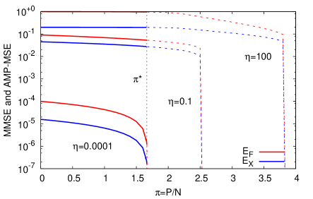
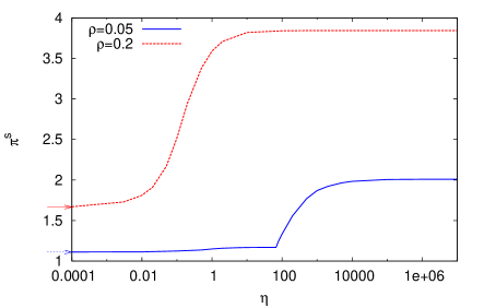
Figure 2: Left: Blind matrix calibration: The predicted MSE $E_{F}$ (for the matrix estimation) and $E_{X}$ (for the signal estimation) corresponding to $\rho=0.2$, $\alpha=0.5$, $\Delta=0$, for three values of $\eta$. MMSE is in full lines, AMP-MSE is in dashed lines. The MMSE jumps abruptly from a finite value to zero at the phase transition point $\pi^{*}$ (251). However, the AMP-MSE matches the MMSE only when the sample complexity is larger than the spinodal transition, that takes place at a larger value $\pi^{s}(\eta)>\pi^{*}$. The AMP-MSE is zero for $\pi>\pi^{s}(\eta)$. Right: We plot the value of the spinodal transition at which the AMP-MSE has a discontinuity as function of $\eta$ for $\alpha=0.5$, $\Delta=0$ and two different values of the sparsity $\rho$. Arrows on the left mark the static transition $\pi^{*}$ and we see that $\lim_{\eta\to 0}\pi^{s}(\eta)=\pi^{*}$. In the limit of dictionary learning, $\eta\to\infty$, the spinodal transition converges to a finite value. Interestingly, for small values of the density, e.g. $\rho=0.05$, we see a sharp phase transition in the threshold $\pi^{s}(\eta)$, in this case at $\eta\approx 68$.

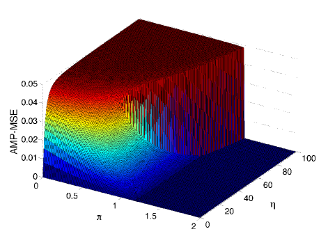
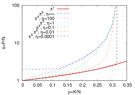
Figure 3: Left: The AMP-MSE of the signal matrix $X$ is plotted against $\pi$ and $\eta$ for the blind matrix calibration at $\rho=0.05$, $\alpha=0.5$ and $\Delta=0$. The transition as a function of the number of samples $\pi$ for fixed matrix uncertainty $\eta$ is always discontinuous in this figure, for larger values of $\eta$ this discontinuity is, however, much more pronounced. Right: The phase diagram of dictionary learning and blind matrix calibration for $\alpha\!=\!0.5$ and $\Delta\!=\!0$. In both cases, the matrix $F$ is identifiable by the Bayes-optimal inference above the full red line $\pi^{*}=\frac{\alpha}{\alpha-\rho}$. However, the system undergoes the spinodal transition $\pi^{s}(\eta)$ shown here with a dashed line for dictionary learning ($\eta\!=\!\infty$) and for blind calibration ($\eta$ finite). Below the spinodal transition, the MMSE is not achieved with AMP. Notice that for $\eta\to 0$ the spinodal line converges to $\pi^{*}$ for $\rho<\rho^{\rm CS}_{\rm BP}$. For all values of $\eta$ the spinodal line diverges as $\rho\to\rho^{\rm CS}_{\rm BP}$. The threshold value $\rho^{\rm CS}_{\rm BP}=0.317$ for $\alpha=0.5$ is the (spinodal) phase transition of pure compressed sensing (when the matrix $F$ is fully known), from Krzakala et al. (2012). Notice also that in the limit of learning a dictionary with a very small sparsity, $\eta\to\infty$ and $\rho\to 0$, the spinodal line converges to $\pi^{s}=2$ whereas the information theoretic transition is at $\pi=1$. Such a gap in the low $\rho$ behavior is striking.

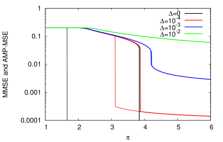
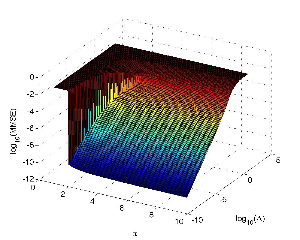
Figure 4: Dictionary learning with noisy measurements. Left: The MMSE (dashed lines) and the AMP-MSE (full lines) for the signal matrix $X$ as a function of the number of samples $P=\pi N$ for $\alpha=0.5$, $\rho=0.2$ for various values of the measurement noise $\Delta$. The behavior is qualitatively the same as for the noiseless case, the only difference is that the MMSE at $\pi>\pi^{*}(\Delta)$, and the AMP-MSE at $\pi>\pi^{s}(\Delta)$ are no longer strictly zero but rather $O(\Delta)$. If the additive noise $\Delta$ is large enough, however, the phase transition disappears and the MMSE$=$AMP-MSE is continuous (this is the case in this plot for $\Delta=10^{-2}$). Right: A surface plot of the MMSE of the signal $E_{X}$ in the $\Delta$, $\pi$-plane in the case $\alpha=0.5$ and $\rho=0.2$. Notice how the sharp transition disappears at large noise where it is replaced by a smooth evolution of the MMSE.

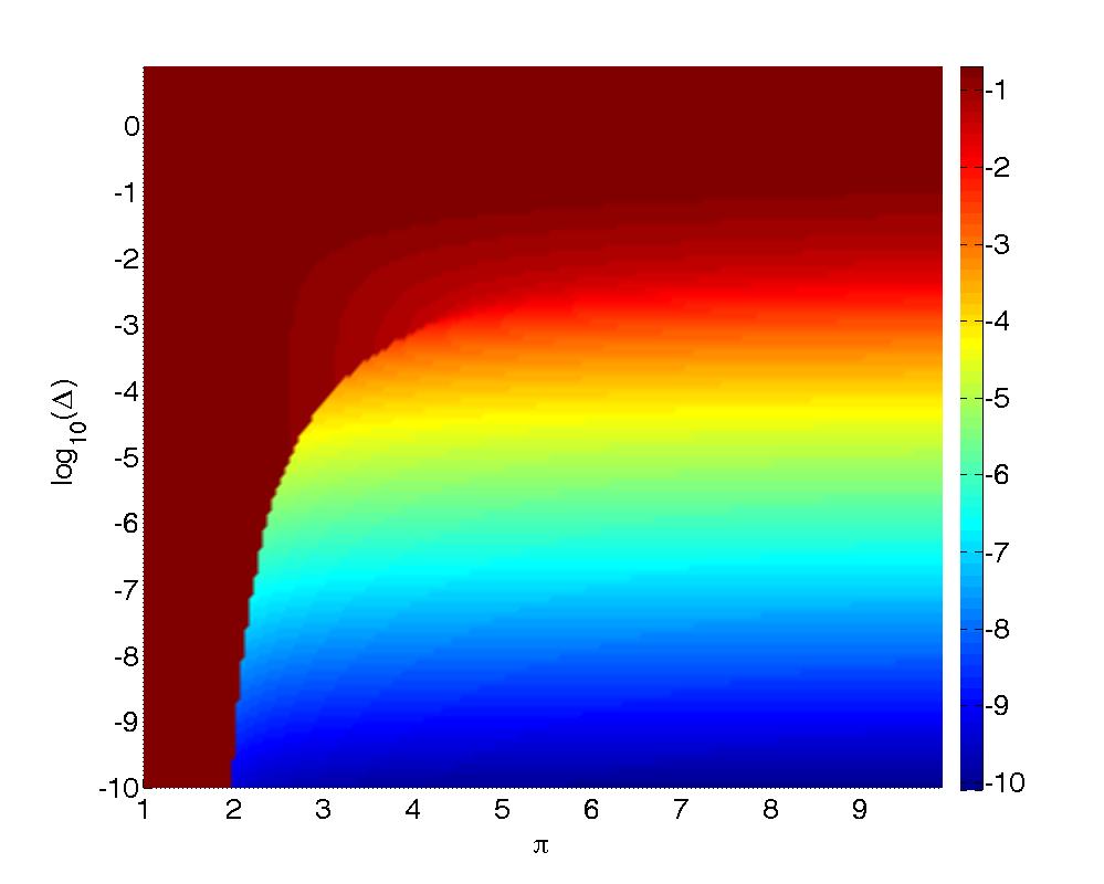
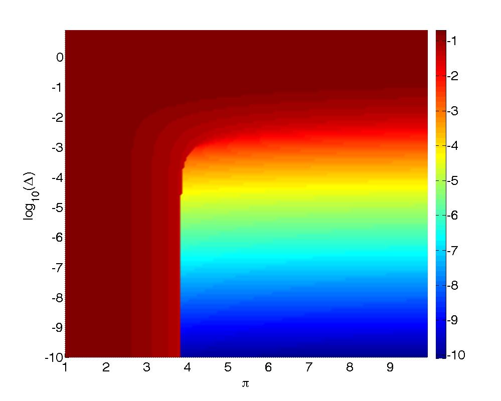
Figure 5: Comparison of the MMSE (left) to the AMP-MSE (right) for noisy dictionary learning with $\alpha=0.5$ and $\rho=0.2$, the MSE of the signal matrix $X$ is plotted on the $\Delta$, $\pi$-plane. The color-scale is in decadic logarithm of the MSEs. We clearly see the region where MMSE$<$AMP-MSE and the one where the two are equal.

Due to the close link between the two problems, we shall described the results for dictionary learning together with the case of blind matrix calibration. In both these cases we are typically trying to learn (calibrate) an overcomplete dictionary $\alpha<1$ and a sparse signal $X$ from as few samples $P$ as possible. We hence first plot in Fig. 2 (left) the MSE for $F$ (in red) and for $X$ (in blue) as a function of $\pi=P/N$ and fixed (representative) value of undersampling ratio $\alpha=0.5$, and density $\rho=0.2$ in zero (or negligible) measurement noise, $\Delta=0$. We consider several values of matrix uncertainty $\eta$ (the larger the value the less we know about the matrix). The AMP-MSE achieved from the uninformative initialization is depicted in dashed lines, the MMSE achieved in this zero noise case from the planted (informative) initialization is in full lines.

Fig. 2 (right) shows the value of the spinodal transition $\pi^{s}$ as a function of the matrix uncertainty $\eta$. We see that, as expected, $\lim_{\eta\to 0}\pi^{s}(\eta)=\pi^{*}$. A result that is less intuitive is that the large $\eta$ limit is also well defined and finite $\lim_{\eta\to\infty}\pi^{s}(\eta)=\pi^{s}_{\rm DL}<0$. This means that even in the dictionary learning where no prior information about the matrix elements is available the dictionary is identifiable with AMP for large system sizes above the spinodal transition $\pi^{s}_{\rm DL}$.

In Fig. 2 (right) we also see an interesting behavior in the function $\pi^{s}(\eta)$ for low values of $\rho$ - there is a sharp phase transition from low $\eta$ regime, where the AMP-MSE at the transition has a weak discontinuity towards a relatively low value of MSE, and a high $\eta$ regime where the discontinuity is very abrupt towards a value of MSE that is close to the completely uninformative value. This behavior is also illustrated in Fig. 3 (left) where we plot the AMP-MSE as a function of $\pi$ and $\eta$ (for fixed $\rho=0.05$, $\alpha=0.5$, $\Delta=0$).

Fig. 3 (right) depicts the phase diagram of dictionary learning ($\eta\to\infty$) and blind matrix calibration (finite $\eta$) we plot the static threshold $\pi^{*}$ ($\eta$-independent) above which the matrix $F$ is identifiable in full red, and the spinodal threshold $\pi^{s}$ (for various values of $\eta$) above which the AMP identifies asymptotically the original matrix $F$ is dashed line. Notice that $\pi^{s}(\rho)$ diverges as $\rho\to\rho^{\rm CS}_{\rm BP}$, where $\rho^{\rm CS}_{\rm BP}$ is the AMP phase transition in compressed sensing, see e.g. Krzakala et al. (2012). This is expected as for $\rho>\rho^{\rm CS}_{\rm BP}$ the sparse signal cannot be recovered with AMP even if the matrix $F$ is fully known.

From now on (also in following subsections) we will discuss only the case $\eta\to\infty$ when no prior information about the dictionary $F$ is available. In Fig. 4 (left) we illustrate the results for dictionary learning with non-zero measurement noise. The situation is qualitatively similar to what happens in noisy compressed sensing Krzakala et al. (2012). The first order phase transition is becoming weaker as the noise grows, until some value $\Delta^{*}$ above which there is no phase transition anymore and the AMP-MSE$=$MMSE for the whole range of $\pi$. In Fig. 4 (right) we then plot the AMP-MSE and the MMSE of the signal $X$ as a function of the noise variance $\Delta$ and $\pi$ for $\alpha=0.5$ and $\rho=0.2$. This surface plot demonstrates how the sharp transition disappears and is replaced by a continuous evolution of the MSE when the noise is large. This MMSE is compared to the AMP-MSE for the same case in Fig. 5.

Phase diagram for sparse PCA

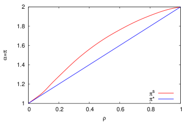
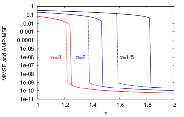
Figure 6: Phase diagram for sparse PCA. Left: Spinodal transition $\pi^{s}$ (upper red, where AMP-MSE goes to zero) and the optimal Bayes inference transition (lower blue, $\pi^{*}=\alpha^{*}=1+\rho$, where MMSE goes to zero) lines in zero measurement noise and when $\alpha=\rho$. Right: AMP-MSE and MMSE of the sparse matrix $X$ in sparse PCA for $\rho=0.5$, $\Delta=10^{-10}$ and several values of ratio $\alpha$ as a function of $\pi$.

Sparse PCA as we set it in Section I.4 is closely related to dictionary learning. Except that from the three sizes of matrices $M$, $N$ and $P$ the smallest one is the $N$ – corresponding to the matrix $Y$ to be of relatively low rank. Hence for sparse PCA we should only really consider $\alpha>1$, $\pi>1$.

Behavior of the state evolution is for this range of parameters qualitatively very similar to the one we just observed in the previous section. In Fig. 6 left we treat the case of $M=P$, i.e. $\pi=\alpha$, with zero measurement noise, and compute the smallest value for which the matrices $F$ and $\rho$-sparse $X$ are recoverable for a given $\rho$. Just as in the dictionary learning we obtain that the Bayes optimal MMSE is zero everywhere above the counting bound $\pi=\alpha>1+\rho$, blue line in Fig. 6 left. The AMP-MSE is, however, zero only above the spinodal line, depicted in red in the figure. The gap between the two lines is not very large in this case.

The right part of Fig. 6 shows the AMP-MSE and the MMSE of the signal matrix $X$ for measurement noise variance $\Delta=10^{-10}$ and density $\rho=0.5$.

Phase diagram for blind source separation

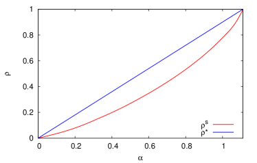
Figure 7: Blind source separation. At the measurement noise $\Delta=0$, $\pi=10$ we plot the spinodal $\rho^{s}$ as a function of $\alpha$. Above this line AMP-MSE$>0$, whereas below this line AMP-MSE$=0$. The static transition line is $\rho^{*}=0.9\alpha$.

In blind source separation, $P$ corresponds to the length of the signal, $N$ is the number of sources, and $M$ the number of sensors. Typically the signal is very long, i.e. one has $P\gg N$ and $P\gg M$. The particularly interesting case is when there is more sources than sensors $\alpha<1$ in that case the signal can be reconstructed only if the density of the signal $\rho$ is smaller than a certain value. The counting bound gives us $\rho<\alpha(\pi-1)/\pi$ and this also corresponds to the value under which the MMSE drops to zero under zero measurement noise. As in the previous case also here we observe a first order phase transition and with AMP we can reach zero error (in the noiseless case) only below $\rho^{s}$ that we depict for $\pi=10$ as a function of $\alpha$ in Fig. 7.

VI.2 Low rank matrix completion

In the remaining examples we treat cases in which neither $F$ nor $X$ are sparse, $\rho=1$, we start with low rank matrix completion.

In matrix completion the output function $g_{\rm out}$ is eq. (244) for the known matrix elements $\mu l$ (there is $\epsilon MP$ of them), and $g_{\rm out}(\omega,y,V)=0$ for the unknown elements $\mu l$ (there is $(1-\epsilon)MP$ of them). The input function $f_{X}$ (242) for non-sparse matrix $X$, $\rho=1$, becomes

$$f_{X}(\Sigma,T)=\frac{\overline{X}\Sigma+T\sigma}{\Sigma+\sigma}\,.$$ (253)

In the state evolution, using the Nishimori identities, we then have

$$\hat{m}^{t}=\frac{\epsilon}{\Delta+\overline{X}^{2}+\sigma-m_{F}^{t}m_{X}^{t}}\,,$$ (254)

where $\epsilon$ is the fraction of known elements of $Y$. Moreover for the input function (253) the state evolution equation for $m_{X}$ becomes

$$m_{X}^{t+1}=\frac{\overline{X}^{2}+(\overline{X}^{2}+\sigma)\sigma\alpha m_{F}^{t}\hat{m}^{t}}{1+\sigma\alpha m_{F}^{t}\hat{m}^{t}}\,.$$ (255)

The equation for $m_{F}$ is the one of (247).

It is instrumental to analyze the local stability of the informative and the uninformative initialization for low rank matrix completion. For the informative initialization we consider $m_{X}^{t}=1-\delta_{X}^{t}$, and $m_{F}^{t}=1-\delta_{F}^{t}$, where $\delta_{X}^{t}$, and $\delta_{F}^{t}$ are small positive numbers. The state evolution update equations at zero noise $\Delta=0$ lead to $\delta_{X}^{t+1}=(\delta_{X}^{t}+\delta_{F}^{t})/(\epsilon\alpha)$, and $\delta_{F}^{t+1}=(\delta_{X}^{t}+\delta_{F}^{t})/(\epsilon\pi)$. The largest eigenvalue of this $2\times 2$ system is $(\alpha+\pi)/(\epsilon\alpha\pi)$ and hence the informative fixed point is stable for $\epsilon>\epsilon^{*}=(\alpha+\pi)/(\alpha\pi)$, which coincides with the counting bound eq. (28). This means that for $\epsilon>\epsilon^{*}$ the noiseless matrix completion, the matrices $F$ and $X$ can be recovered without error (asymptotically).

For the uninformative initialization we consider $m_{X}^{t}=\delta_{X}^{t}$, and $m_{F}^{t}=\delta_{F}^{t}$, where $\delta_{X}^{t}$, and $\delta_{F}^{t}$ are again small positive numbers. This time the state evolution equations give $\delta_{F}^{t+1}=\pi\epsilon\delta_{X}^{t}/(1+\Delta)$ and $\delta_{X}^{t+1}=\alpha\epsilon\delta_{F}^{t}/(1+\Delta)$. Hence the uninformative fixed point is stable for $\epsilon<(\Delta+1)/\sqrt{\pi\alpha}$. This can indeed be verified in Fig. 8.

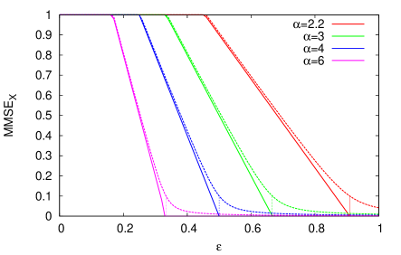
Figure 8: Low rank matrix completion. The MMSE of the signal matrix $X$ is plotted for $\alpha=\pi$ (for four different values of this parameter) in the noiseless (full line) and noisy (dashed lines), with $\Delta=10^{-2}$, cases. In zero noise there is a second order phase transition which coincides with the counting bound, eq. (28), marked by short vertical lines. With non-zero noise there is no phase transition.

In matrix completion we treat matrices $Y$ of low rank, hence $N$ is much smaller than both $P$ and $M$. The main questions concerns the fraction $\epsilon$ of elements that need to be known in order for the recovery of $X$ and $F$ to be possible. In this case we did not identify first order phase transition, as a result we have MMSE$=$AMP-MSE. At zero measurement noise we observed a phase transition from a phase of perfect recovery to a phase with positive MMSE, its position coincides with the counting bound (28), $\epsilon^{*}=(\alpha+\pi)/{\alpha\pi}$. With non-zero measurement noise, in the scaling of noise and rank we consider in this paper, the behavior of MMSE as a function of the other parameters is smooth and derivable (no phase transition). In Fig. 8 we plot an example of the MMSE as a function of the fraction of known elements $\epsilon$ for squared matrix $Y$, i.e $\alpha=\pi$. We generated the signal elements with zero mean and unit variance, $\overline{X}=0$, $\sigma=1$.

Our analysis suggest that compared to the cases with non-zero sparsity the low-rank matrix completion is a much easier problem, at least in the random setting considered in the present paper. The fact that the “counting” threshold can be saturated or close to saturated in the noiseless case by several algorithms can be seen e.g. in the data presented in Parker et al. (2014).

VI.3 Robust PCA

The input functions are the eq. (242) for matrix $F$ and eq. (253) for matrix $X$. In robust PCA as defined by (30) we get for the output function

$$g_{\rm out}(\omega,y,V)=\frac{y-\omega}{V}\left[1-\epsilon\frac{\Delta_{s}}{\Delta_{s}+V}-(1-\epsilon)\frac{\Delta_{l}}{\Delta_{l}+V}\right]\,.$$ (256)

The state evolution in the Bayes-optimal setting, i.e. using the Nishimori identities, becomes

$$\hat{m}^{t}=\frac{1}{\overline{X}^{2}+\sigma-m_{F}^{t}m_{X}^{t}}\left[1-\epsilon\frac{\Delta_{s}}{\Delta_{s}+\overline{X}^{2}+\sigma-m_{F}^{t}m_{X}^{t}}-(1-\epsilon)\frac{\Delta_{l}}{\Delta_{l}+\overline{X}^{2}+\sigma-m_{F}^{t}m_{X}^{t}}\right]\,.$$ (257)

Equation for $m_{F}^{t}$ is (247), and for $m_{X}^{t}$ is (255).

In robust PCA the informative initialization is again $m_{X}^{t}=1-\delta_{X}^{t}$, and $m_{F}^{t}=1-\delta_{F}^{t}$, where $\delta_{X}^{t}$, and $\delta_{F}^{t}$ are small positive numbers. For small noise $\Delta_{s}$ and $\Delta_{l}=O(1)$ the corresponding fixed point is stable under the same conditions as for low rank matrix completion, i.e. for $\epsilon>\epsilon^{*}=(\alpha+\pi)/(\alpha\pi)$.

The uninformative fixed point is $m_{X}^{t}=\delta_{X}^{t}$, and $m_{F}^{t}=\delta_{F}^{t}$, where $\delta_{X}^{t}$, and $\delta_{F}^{t}$ are again small positive numbers. This evolves as $\delta_{X}^{t+1}=\alpha\delta_{F}^{t}\hat{m}$, $\delta_{F}^{t+1}=\pi\delta_{X}^{t}\hat{m}$, with $\hat{m}=(1+\delta_{s}=\epsilon\Delta_{l}-\epsilon\Delta_{s})/[(1+\Delta_{s})(1+\Delta_{l})]$ in this limit. Hence for instance for $\Delta_{s}\to 0$, $\Delta_{l}=1$ and $\pi=\alpha$ we have that the uninformative fixed point is stable for $\epsilon<2/\alpha-1$, which again corresponds to what we observe in Fig. 9.

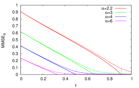
Figure 9: MMSE of the matrix $X$ in robust PCA with $\alpha=\pi$ in the noiseless (full line, $\Delta_{s}=0$, $\Delta_{l}=1$), and the noisy (dashed lines, with $\Delta_{s}=10^{-2}$, $\Delta_{l}=1$) cases. The situation is not very different from low rank matrix completion. Indeed in the noiseless case there is a second order phase transition and the MMSE is zero beyond the counting bound, marked by short vertical lines. In presence of noise there is no phase transition.

In the example of Fig. 9 we plot the MMSE as a function of the fraction of undistorted elements $\epsilon$ in the case of squared matrix $Y$, $\alpha=\pi$, the variance of the large distortions $\Delta_{l}=1$ and two different values of the small measurement noise $\Delta_{s}$. We see a second order phase transition at the counting bound for $\Delta_{s}=0$ and a smooth decay of the MMSE for $\Delta_{X}>0$.

It is interesting to compare how well robust PCA can be solved with respect to the matrix completion. In both cases $\epsilon$ is the fraction of known elements. The difference is that in matrix completion their position is known, whereas in robust PCA it is not. Intuitively the R-PCA should thus be a much harder problem. This is not confirmed in our analysis that instead suggest that robust PCA is as easy as matrix completion, since the zero noise phase transitions in the two coincide. Moreover, whereas at $\epsilon\to 0$ there is no information left in matrix completion (that is why the MMSE$=1$), in robust PCA the largely distorted elements can still be explored and the MMSE$<1$. Note, however, that algorithmically it seems less easy to saturate this theoretical asymptotic performance in R-PCA, see e.g. Figure 7 in Parker et al. (2014).

VI.4 Factor analysis

In factor analysis, the input functions $f_{F}$ and $f_{X}$ are the same as the dictionary learning (242) at $\rho=1$. The output function (56) for factor analysis (31) is given by

$$g_{\rm out}(\omega_{\mu l},y_{\mu l},V_{\mu})=\frac{y_{\mu l}-\omega_{\mu l}}{{\psi}_{\mu}+V_{\mu l}},$$ (258)

where $\psi_{\mu}$ is the variance of the $\mu$-th component of the unique factor. The variance of unique factor $\psi_{\mu}$ depends here on the index $\mu$ and does not on the index $l$, which leads to a slight modification in the derivation of the state evolution from section V.1. For simplicity, we assume that $\psi_{\mu}$’s are known; in practice, these should be estimated by the expectation and maximization scheme in conjunction with GAMP. Then, we obtain, on the Nishimori line

$$\hat{m}_{\mu}^{t} =\frac{1}{\psi_{\mu}+Q^{0}_{F,\mu}(\overline{X}^{2}+\sigma)-m^{t}_{F,\mu}m^{t}_{X}}.$$ (259)

$$m_{F,\mu}^{t+1} =\frac{\pi Q^{0}_{F,\mu}m_{X}^{t}\hat{m}^{t}_{\mu}}{1+\pi Q^{0}_{F,\mu}m_{X}^{t}\hat{m}_{\mu}^{t}},$$ (260)

$$m_{X}^{t+1} =\frac{\alpha\sigma^{2}\langle{m_{F,\mu}^{t}\hat{m}_{\mu}^{t}}\rangle_{\mu}}{1+\alpha\sigma\langle{m_{F,\mu}^{t}\hat{m}_{\mu}^{t}}\rangle_{\mu}},$$ (261)

where $\langle\cdot\rangle_{\mu}$ means the average over $\psi_{\mu}$, the variance of the elements of the matrix $F$ is denoted $Q_{F,\mu}^{0}$.

To analytically solve (261), one has to specify the distributions of $\psi_{\mu}$ and $Q_{F,\mu}^{0}$. We set $Q_{F,\mu}^{0}=Q_{F}^{0}=1$ for all $\mu$, and suppose a two-peak distribution for $\psi$ as

$$P_{\psi}(\psi)=\epsilon\delta(\psi-\psi_{1})+(1-\epsilon)\delta(\psi-\psi_{2}).$$ (262)

Let us also assume $\overline{X}=0$ and $\sigma=1$. In this case the state evolution can be summarized as

$$m_{F1} =\frac{\pi m_{X}\hat{m}_{1}^{t}}{1+\pi m_{X}\hat{m}_{1}^{t}},~{}~{}~{}m_{F2}=\frac{\pi m_{X}\hat{m}_{2}^{t}}{1+\pi m_{X}\hat{m}_{2}^{t}}$$ (263)

$$m_{X} =\frac{\alpha\{\epsilon m_{F1}\hat{m}_{1}^{t}+(1-\epsilon)m_{F2}\hat{m}_{2}^{t}\}}{1+\alpha\{\epsilon m_{F1}\hat{m}_{1}^{t}+(1-\epsilon)m_{F2}\hat{m}_{2}^{t}\}},$$ (264)

where

$$\hat{m}_{1}^{t}=\frac{1}{\psi_{1}+1-m_{F1}m_{X}},~{}~{}~{}\hat{m}_{2}^{t}=\frac{1}{\psi_{2}+1-m_{F2}m_{X}}.$$ (265)

The total MMSE is given by $E_{F}=1-(\epsilon m_{F1}+(1-\epsilon)m_{F2})$ and $E_{X}=1-m_{X}$. Fig. 10 (left) shows the $\pi$-dependence of the MMSE at $\alpha=2$, $\psi_{1}=0.5$, and $\psi_{2}=2$ for $\epsilon=0$, 0.5, 0.9 and 1.

We analyze again the stability of the uninformative fixed point, $(m_{X},m_{F_{1}},m_{F_{2}})=(0,0,0)$, of the state evolution. Small positive numbers $\delta_{X}$, $\delta_{F_{1}}$, and $\delta_{F_{2}}$ that give the uninformative initialization $m_{X}=\delta_{X}$, $m_{F_{1}}=\delta_{F_{1}}$, and $m_{F_{2}}=\delta_{F_{2}}$ evolve under the state evolution as

$$\delta_{F_{1}}^{t+1} =\frac{\pi\delta_{X}^{t}}{\psi_{1}+1},~{}~{}~{}\delta_{F_{2}}^{t+1}=\frac{\pi\delta_{X}^{t}}{\psi_{2}+1},$$ (266)

$$\delta_{X}^{t+1} =\alpha\pi\Big{[}\frac{\epsilon}{(\psi_{1}+1)^{2}}+\frac{1-\epsilon}{(\psi_{2}+1)^{2}}\Big{]}\delta_{X}^{t}.$$ (267)

These expressions indicate that the uninformative fixed point becomes unstable when $\alpha\pi\Big{[}\frac{\epsilon}{(\psi_{1}+1)^{2}}+\frac{1-\epsilon}{(\psi_{2}+1)^{2}}\Big{]}>1$. The critical values of $\pi$ given by this condition coincides with the transition point where the MMSE departs from 1 shown in Fig. 10 (left). As an example of $\epsilon$-dependence, we show the MMSE of $X$ at $\psi_{1}=10^{-2}$, $\psi_{1}=10^{-5}$ and $\psi_{2}=1$ for four different values of $\alpha=\pi$ in Fig. 10 (right). Consistently with our analysis, in these cases the uninformative initialization is always unstable.

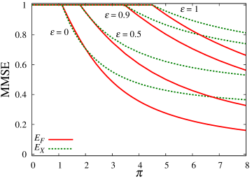
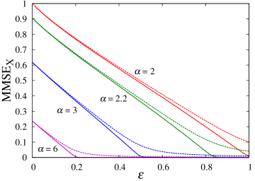
Figure 10: Left: MMSE in factor analysis with $\psi_{1}=0.5$ and $\psi_{2}=2$, $\alpha=2$. Right: MMSE of the signal matrix $X$ in factor analysis at four different values of $\alpha=\pi$ at $\psi_{1}=10^{-2}$ and $\psi_{2}=1$ (dashed lines), and $\psi_{1}=10^{-5}$ and $\psi_{2}=1$ (solid lines).

The transition associated with the stability of the informative fixed point occurs only when at least one of $\psi$s tends to be zero. For instance when $\psi_{1}=0$, the informative initialization corresponds to $\delta_{F_{1}}=1-m_{F_{1}}$ and $\delta_{X}=1-m_{X}$ that are given by

$$\delta_{F_{1}}^{t+1}=\frac{\delta_{X}^{t}+\delta_{F_{1}}^{t}}{\pi},~{}~{}~{}\delta_{X}^{t+1}=\frac{\delta_{F_{1}}^{t}+\delta_{X}^{t}}{\alpha\epsilon}$$ (268)

without depending on $\psi_{2}$. These expressions mean that when $\epsilon>\epsilon^{*}=\pi/[\alpha(\pi-1)]$, the informative fixed point is stable, consistently with Fig. 10 (right).

The state evolution of factor analysis for the two-peak case is qualitatively similar to that of robust PCA and low rank matrix completion, but the values of the phase transition points differ.

VII Discussion and Conclusions

In this paper we have analyzed various examples of the matrix factorization problem. We obtain a matrix $Y$ that is an element-wise noisy measurement of an unknown matrix $Z=FX$, where both $Y$, and $Z$ are $M\times P$ matrices, $F$ is a $M\times N$ matrix, and $X$ is a $N\times P$ matrix. We have considered the computational tractability of this problem in the large size limit $N\to\infty$ while $\pi=P/N=O(1)$, and $\alpha=M/N=O(1)$. Our analysis concerns the teacher-student scenario where $X$ and $F$ are generated with random independent elements of some known probability distributions and we employ the Bayes-optimal inference scheme to recover $F$ and $X$ from $Y$.

Let us summarize our contribution: We derived the approximate message passing algorithm for matrix factorization. One version of the algorithm —for calibration and dictionary learning— was reported in Krzakala et al. (2013), and a very related algorithm called Big-AMP was discussed by Parker et al. (2013, 2014). This algorithm is derived from belief propagation. We have presented the AMP for matrix factorization in several forms in Sections III.1, and III.2. We have also discussed simplifications that arise in the Bayes-optimal setting when we can use the Nishimori identities (Section III.3), or when the matrix is large and one uses self-averaging of some of the quantities appearing in GAMP (Section III.4). We focused on the theoretical properties of the AMP algorithm, for a robust practical implementation we refer the reader to the works Parker et al. (2013, 2014) that include a very complete report on its performance on a range of benchmarks.

Next to the AMP algorithm we have also derived the corresponding Bethe free entropy in Section IV. The Bethe free entropy evaluated at a fixed point of the GAMP equations approximates the log-likelihood of the corresponding problem. We mainly use it in situations when we have more than one fixed point of GAMP, it is then the one with the largest values of the Bethe entropy that asymptotically given the MMSE of the Bayes-optimal inference. We also derived a variational Bethe free entropy in Section IV.2. This is a useful quantity that can serve in controlling the convergence of the AMP approach. Alternatively, a direct maximization of this expression is a promising algorithm itself (see Krzakala et al. (2014) for an investigation of this idea for compressed sensing).

The AMP algorithm for matrix factorization is amenable to asymptotic analysis via the state evolution technique that was carried out rigorously for approximate message passing in compressed sensing Bayati & Montanari (2011). We derive the state evolution analysis for matrix factorization using tools of statistical mechanics. In particular we use two approaches leading to equivalent results the cavity method (Section V.1) and the replica method (Section V.2). Our derivation of the state evolution is not rigorous, but we conjecture that it is nevertheless asymptotically exact as is the case in many other systems of this type including the compressed sensing. The main result of this state evolution are simple iterative equations that provide a way to compute the MMSE of the Bayes-optimal inference as well as the MSE reached theoretically in the large size limit by the AMP algorithm. The rigorous proof of the formulas derived in this paper is obviously an important topic for future work.

The main results of this paper concern analysis of MMSE and AMP-MSE for various interesting examples of the matrix factorization problem. We analyze the asymptotic phase diagrams for dictionary learning, blind matrix calibration, sparse PCA, blind source separation, matrix completion, robust PCA and factor analysis. Earlier results on this analysis appeared in Krzakala et al. (2013); Sakata & Kabashima (2013). We find that when one of the matrices $F$ or $X$ is sparse the problems undergo a first order phase transition which is related to an interesting algorithmic barrier known for instance from compressed sensing Krzakala et al. (2012).

It is a generic observation that for most of the problems we analyzed the theoretically achievable performance is much better than the one achievable by existing algorithms. The AMP algorithm should be able to match this performance for very large systems which is the most exciting perspective for further development of this work. If successful it could lead to an algorithmic revolution in various application of the matrix factorization.

In this paper we concentrate on the theoretical analysis and not on the performance of the algorithm itself. Some studies of the performance of some versions of the algorithm can be find in Krzakala et al. (2013); Parker et al. (2014). We, however, observed that the performance depends strongly on the implementation details and we did not yet found a way to match the theoretically predicted performance for systems of treatable (practical) size in all cases.

It is worth discussing some of these algorithmic issues in this conclusion. One of the main problems it that the GAMP algorithm with parallel update presents instabilities that drive its evolution away from the so-called Nishimori line; see a recent study of this issue in the compressed sensing problem Caltagirone et al. (2014). This can be seen even in the state evolution when we do not assume explicitly that the result of the Bayes-optimal inference corresponds to a fixed point that belongs to the Nishimori line. There are ways how to avoid these issues, e.g. we observed that the difficulties basically disappear when the sequential update of the message passing algorithm from Section III.1 is used instead of the parallel one. This, however, does not scale very well with the systems size and our results were hence spoiled by very strong finite size effects. When learning the $M\times N$ matrix $F$, and the $N\times P$ matrix $X$ we also often observed that a (very small) number of the $P$ signals $X_{l}$ were not correctly reconstructed, and these “rogue” vectors in $X_{l}$ were polluting the reconstruction of $F$. An exemple of these finite size effects can be observed in Krzakala et al. (2013).

In the work of Parker et al. (2013, 2014) a part of the problems with convergence of the corresponding algorithm was mitigated by adaptive damping (though maybe with not the most suitable cost function, see Sec. IV) and expectation maximization learning. Why this is helpful is theoretically explained in the recent work Caltagirone et al. (2014) for compressed sensing. However, the implementation of Parker et al. (2014) does not match the theoretical performance predicted in this paper either (we have explicitly tried for the dictionary learning and robust PCA examples). This shows that more work is needed in order to reach a practical algorithm able to achieve the prediction at moderate sizes. A more proper understanding of these problems, and further developments of the algorithm are therefore the main direction of our future work.

variable nodes	definition	$X$	definition	$F$
variables for elements	(1)	$X_{il}$	(1)	$F_{\mu i}$
true elements	(7)	$X^{0}_{il}$	(9)	$F^{0}_{\mu i}$
prior distribution	(4)	$P_{X}(X_{il})$	(3)	$P_{F}(F_{\mu i})$
incoming BP message	(43)	${\tilde{m}}_{\mu l\to il}(X_{il})$	(44)	${\tilde{n}}_{\mu l\to\mu i}(F_{\mu i})$
outgoing BP message	(41)	$m_{il\to\mu l}(X_{il})$	(42)	$n_{\mu i\to\mu l}(F_{\mu i})$
approximate-BP mean	(45)	${\hat{x}}_{il\to\mu l}$	(47)	${\hat{f}}_{\mu i\to\mu l}$
approximate-BP variance	(46)	$c_{il\to\mu l}$	(48)	$s_{\mu i\to\mu l}$
incoming-BP mean	(59)	$B_{\mu l\to il}$	(62)	$R_{\mu l\to\mu i}$
incoming-BP variance	(60)	$A_{\mu l\to il}$	(63)	$S_{\mu l\to\mu i}$
mean-input function	(66)	$f_{X}$	(67)	$f_{F}$
variance-input function	(66)	$f_{c}$	(67)	$f_{s}$
incoming mean	(88)	$T_{il}$	(89)	$W_{\mu i}$
incoming variance	(88)	$\Sigma_{il}$	(89)	$Z_{\mu i}$
GAMP estimate of mean	(102)	${\hat{x}}_{il}$	(103)	${\hat{f}}_{\mu i}$
GAMP estimate of variance	(102)	$c_{il}$	(103)	$s_{\mu i}$
SE magnetization	(160)	$m_{X}$	(160)	$m_{F}$
SE overlap	(161)	$q_{X}$	(161)	$q_{F}$
SE variance	(162)	$Q_{X}-q_{X}$	(162)	$Q_{F}-q_{F}$

factor nodes	definition	output
matrix to factorize	(1)	$z_{\mu l}$
output	(2)	$y_{\mu l}$
output probability	(2)	$P_{\rm out}(y_{\mu l}|z_{\mu l})$
output realization function	(10)	$h(z,w)$
cavity variance of $z_{\mu l}$	(53)	$V_{\mu il}$
cavity estimation of $z_{\mu l}$	(54)	$\omega_{\mu il}$
output function	(56)	$g_{\rm out}(\omega,y,V)$
variance of $z_{\mu l}$	(90)	$V_{\mu l}$
estimation of $z_{\mu l}$	(91)	$\omega_{\mu l}$
SE output $q$	(169)	$\hat{q}$
SE output $\chi$	(168)	$\hat{\chi}$
SE output $m$	(177)	$\hat{m}$

Table 1: Glossary of notations with the number of equation where the quantity was defined or first used.

References

- Bengio et al. 2013 Bengio Y., Courville A. & Vincent P. Representation learning: A review and new perspectives. Pattern Analysis and Machine Intelligence, IEEE Transactions on 35, 1798–1828 (2013).
- LeCun et al. 2015 LeCun Y., Bengio Y. & Hinton G. Deep learning. Nature 521, 436–444 (2015).
- Olshausen et al. 1996 Olshausen B. A. et al. Emergence of simple-cell receptive field properties by learning a sparse code for natural images. Nature 381, 607–609 (1996).
- Olshausen & Field 1997 Olshausen B. A. & Field D. J. Sparse Coding with an Overcomplete Basis Set: A Strategy Employed by V1. Vision Research 37, 3311 (1997).
- Kreutz-Delgado et al. 2003 Kreutz-Delgado K. et al. Dictionary learning algorithms for sparse representation. Neural computation 15, 349–396 (2003).
- Zou et al. 2006 Zou H., Hastie T. & Tibshirani R. Sparse principal component analysis. Journal of computational and graphical statistics 15, 265–286 (2006).
- Belouchrani et al. 1997 Belouchrani A., Abed-Meraim K., Cardoso J.-F. & Moulines E. A blind source separation technique using second-order statistics. Signal Processing, IEEE Transactions on 45, 434–444 (1997).
- Candès & Recht 2009 Candès E. J. & Recht B. Exact matrix completion via convex optimization. Foundations of Computational mathematics 9, 717–772 (2009).
- Candès & Tao 2010 Candès E. J. & Tao T. The power of convex relaxation: Near-optimal matrix completion. Information Theory, IEEE Transactions on 56, 2053–2080 (2010).
- Candès et al. 2011 Candès E. J., Li X., Ma Y. & Wright J. Robust principal component analysis? Journal of the ACM (JACM) 58, 11 (2011).
- Donoho et al. 2009 Donoho D. L., Maleki A. & Montanari A. Message-passing algorithms for compressed sensing. Proc. Natl. Acad. Sci. 106, 18914–18919 (2009).
- Mézard et al. 1987 Mézard M., Parisi G. & Virasoro M. A. Spin-Glass Theory and Beyond, vol. 9 (World Scientific, Singapore, 1987).
- Mézard & Montanari 2009 Mézard M. & Montanari A. Information, Physics, and Computation (Oxford Press, Oxford, 2009).
- Sakata & Kabashima 2013 Sakata A. & Kabashima Y. Sample complexity of Bayesian optimal dictionary learning. In Information Theory Proceedings (ISIT), 2013 IEEE International Symposium on, 669–673 (2013).
- Krzakala et al. 2013 Krzakala F., Mézard M. & Zdeborová L. Phase diagram and approximate message passing for blind calibration and dictionary learning. In IEEE International Symposium on Information Theory Proceedings (ISIT), 659–663 (2013).
- Schniter et al. 2012 Schniter P., Parker J. & Cevher V. Bilinear Generalized Approximate Message Passing (BiG-AMP) for Matrix Recovery Problem. In Workshop on Information Theory and Applications (ITA), San Diego CA (2012).
- Parker et al. 2013 Parker J., Schniter P. & Cevher V. Bilinear generalized approximate message passing—Part I: Derivation. Signal Processing, IEEE Transactions on 62, 5839–5853 (2013).
- Parker et al. 2014 Parker J., Schniter P. & Cevher V. Bilinear generalized approximate message passing—Part II: Applications. Signal Processing, IEEE Transactions on 62, 5854–5867 (2014).
- Elad 2012 Elad M. Sparse and Redundant Representation Modeling—What Next? Signal Processing Letters 19 (2012).
- Mézard et al. 2002 Mézard M., Parisi G. & Zecchina R. Analytic and Algorithmic Solution of Random Satisfiability Problems. Science 297, 812–815 (2002).
- Ding et al. 2014 Ding J., Sly A. & Sun N. Proof of the satisfiability conjecture for large k. arXiv preprint arXiv:1411.0650 (2014).
- Tanaka 2002 Tanaka T. A statistical-mechanics approach to large-system analysis of CDMA multiuser detectors. IEEE Trans. Infor. Theory 48, 2888–2910 (2002).
- Guo & Verdú 2005 Guo D. & Verdú S. Randomly spread CDMA: Asymptotics via statistical physics. IEEE Trans. Infor. Theory 51, 1983–2010 (2005).
- Montanari & Tse 2006 Montanari A. & Tse D. Analysis of belief propagation for non-linear problems: The example of CDMA (or: How to prove Tanaka’s formula). In Information Theory Workshop, 2006. ITW’06 Punta del Este. IEEE, 160–164 (IEEE, 2006).
- Bayati & Montanari 2011 Bayati M. & Montanari A. The Dynamics of Message Passing on Dense Graphs, with Applications to Compressed Sensing. IEEE Transactions on Information Theory 57, 764 –785 (2011).
- Davenport et al. 2014 Davenport M. A., Plan Y., van den Berg E. & Wootters M. 1-bit matrix completion. Information and Inference 3, 189–223 (2014).
- Davenport & Romberg 2015 Davenport M. & Romberg J. An overview of low-rank matrix recovery from incomplete observations (2015).
- Lesieur et al. 2015 Lesieur T., Krzakala F. & Zdeborová L. MMSE of probabilistic low-rank matrix estimation: Universality with respect to the output channel. arXiv preprint arXiv:1507.03857 (2015).
- Jöreskog 1969 Jöreskog K. G. A general approach to confirmatory maximum likelihood factor analysis. Psychometrika 34, 183–202 (1969).
- Lewicki & Sejnowski 2000 Lewicki M. S. & Sejnowski T. J. Learning overcomplete representations. Neural computation 12, 337–365 (2000).
- Engan et al. 1999 Engan K., Aase S. O. & Husoy J. H. Method of optimal directions for frame design. In Proceedings of the 1999 IEEE International Conference on Acoustics, Speech, and Signal Processing, 2443–2446 (IEEE, 1999).
- Aharon et al. 2006 Aharon M., Elad M. & Bruckstein A. M. K-SVD: An Algorithm for Designing Overcomplete Dictionaries for Sparse Representation. IEEE Transactions on Signal Processing 54, 4311 (2006).
- Michal Aharon 2006 Michal Aharon, Michael Elad A. M. B. On the uniqueness of overcomplete dictionaries, and a practical way to retrieve them. Linear Algebra and its Applications 416, 48–67 (2006).
- Vainsencher et al. 2011 Vainsencher D., Mannor S. & Bruckstein A. M. The Sample Complexity of Dictionary Learning. Journal of Machine Learning Research 12, 3259–3281 (2011).
- Jenatton et al. 2012 Jenatton R., Gribonval R. & Bach F. Local stability and robustness of sparse dictionary learning in the presence of noise. arXiv:1210.0685 (2012).
- Spielman et al. 2013 Spielman D. A., Wang H. & Wright J. Exact recovery of sparsely-used dictionaries. In Proceedings of the Twenty-Third international joint conference on Artificial Intelligence, 3087–3090 (AAAI Press, 2013).
- Arora et al. 2013 Arora S., Ge R. & Moitra A. New algorithms for learning incoherent and overcomplete dictionaries. arXiv preprint arXiv:1308.6273 (2013).
- Agarwal et al. 2013 Agarwal A., Anandkumar A. & Netrapalli P. Exact Recovery of Sparsely Used Overcomplete Dictionaries. arXiv preprint arXiv:1309.1952 (2013).
- Gribonval et al. 2013 Gribonval R., Jenatton R., Bach F., Kleinsteuber M. & Seibert M. Sample complexity of dictionary learning and other matrix factorizations. arXiv preprint arXiv:1312.3790 (2013).
- Lee et al. 1999 Lee T.-W., Lewicki M. S., Girolami M. & Sejnowski T. J. Blind source separation of more sources than mixtures using overcomplete representations. Signal Processing Letters, IEEE 6, 87–90 (1999).
- Zibulevsky & Pearlmutter 2001 Zibulevsky M. & Pearlmutter B. A. Blind source separation by sparse decomposition in a signal dictionary. Neural computation 13, 863–882 (2001).
- Bofill & Zibulevsky 2001 Bofill P. & Zibulevsky M. Underdetermined blind source separation using sparse representations. Signal processing 81, 2353–2362 (2001).
- Georgiev et al. 2005 Georgiev P., Theis F. & Cichocki A. Sparse component analysis and blind source separation of underdetermined mixtures. Neural Networks, IEEE Transactions on 16, 992–996 (2005).
- d’Aspremont et al. 2007 d’Aspremont A., El Ghaoui L., Jordan M. I. & Lanckriet G. R. A direct formulation for sparse PCA using semidefinite programming. SIAM review 49, 434–448 (2007).
- Gribonval et al. 2006 Gribonval R., Lesage S. et al. A survey of sparse component analysis for blind source separation: principles, perspectives, and new challenges. In ESANN’06 proceedings-14th European Symposium on Artificial Neural Networks, 323–330 (2006).
- Candes & Plan 2010 Candes E. J. & Plan Y. Matrix completion with noise. Proceedings of the IEEE 98, 925–936 (2010).
- Keshavan et al. 2010 Keshavan R. H., Montanari A. & Oh S. Matrix completion from a few entries. Information Theory, IEEE Transactions on 56, 2980–2998 (2010).
- Chandrasekaran et al. 2009 Chandrasekaran V., Sanghavi S., Parrilo P. A. & Willsky A. S. Sparse and low-rank matrix decompositions. In Communication, Control, and Computing, 2009. Allerton 2009. 47th Annual Allerton Conference on, 962–967 (IEEE, 2009).
- Yuan & Yang 2009 Yuan X. & Yang J. Sparse and low-rank matrix decomposition via alternating direction methods. preprint (2009).
- Wright et al. 2009 Wright J., Ganesh A., Rao S., Peng Y. & Ma Y. Robust principal component analysis: Exact recovery of corrupted low-rank matrices via convex optimization. In Advances in neural information processing systems, 2080–2088 (2009).
- Rangan & Fletcher 2012 Rangan S. & Fletcher A. K. Iterative estimation of constrained rank-one matrices in noise. In Information Theory Proceedings (ISIT), 2012 IEEE International Symposium on, 1246–1250 (IEEE, 2012).
- Deshpande & Montanari 2014 Deshpande Y. & Montanari A. Information-theoretically Optimal Sparse PCA. arXiv preprint arXiv:1402.2238 (2014).
- Opper & Haussler 1991 Opper M. & Haussler D. Calculation of the Learning Curve of Bayes Optimal Classification Algorithm for Learning a Perceptron With Noise. In In Computational Learning Theory: Proceedings of the Fourth Annual Workshop, 75–87 (Morgan Kaufmann, 1991).
- Iba 1999 Iba Y. The Nishimori line and Bayesian statistics. Journal of Physics A: Mathematical and General 32, 3875 (1999).
- Nishimori 2001 Nishimori H. Statistical Physics of Spin Glasses and Information Processing (Oxford University Press, Oxford, 2001).
- Donoho et al. 2012 Donoho D. L., Javanmard A. & Montanari A. Information-Theoretically Optimal Compressed Sensing via Spatial Coupling and Approximate Message Passing. In Proc. of the IEEE Int. Symposium on Information Theory (ISIT) (2012).
- Mézard et al. 1986 Mézard M., Parisi G. & Virasoro M. A. SK Model: The Replica Solution without Replicas. Europhys. Lett. 1, 77–82 (1986).
- Richardson & Urbanke 2008 Richardson T. & Urbanke R. Modern Coding Theory (Cambridge University Press, 2008).
- Aldous 2001 Aldous D. J. The (2) limit in the random assignment problem. Random Structures & Algorithms 18, 381–418 (2001).
- Montanari 2008 Montanari A. Estimating random variables from random sparse observations. European Transactions on Telecommunications 19, 385–403 (2008).
- Kabashima et al. 2009 Kabashima Y., Wadayama T. & Tanaka T. A typical reconstruction limit of compressed sensing based on Lp-norm minimization. J. Stat. Mech. L09003 (2009).
- Dempster et al. 1977 Dempster A., Laird N. & Rubin D. Maximum Likelihood from Incomplete Data via the EM Algorithm. Journal of the Royal Statistical Society 38, 1 (1977).
- Krzakala et al. 2012 Krzakala F., Mézard M., Sausset F., Sun Y. & Zdeborová L. Probabilistic Reconstruction in Compressed Sensing: Algorithms, Phase Diagrams, and Threshold Achieving Matrices. J. Stat. Mech. (2012).
- Vila & Schniter 2011 Vila J. P. & Schniter P. Expectation-Maximization Bernoulli-Gaussian Approximate Message Passing. In Proc. Asilomar Conf. on Signals, Systems, and Computers (Pacific Grove, CA) (2011).
- Donoho et al. 2010 Donoho D., Maleki A. & Montanari A. Message passing algorithms for compressed sensing: I. motivation and construction. In IEEE Information Theory Workshop (ITW), 1 –5 (2010).
- Rangan 2011 Rangan S. Generalized approximate message passing for estimation with random linear mixing. In IEEE International Symposium on Information Theory Proceedings (ISIT), 2168 –2172 (2011).
- Kschischang et al. 2001 Kschischang F. R., Frey B. & Loeliger H.-A. Factor graphs and the sum-product algorithm. IEEE Trans. Inform. Theory 47, 498–519 (2001).
- Thouless et al. 1977 Thouless D. J., Anderson P. W. & Palmer R. G. Solution of ‘Solvable Model of a Spin-Glass’. Phil. Mag. 35, 593–601 (1977).
- Rangan 2010 Rangan S. Estimation with random linear mixing, belief propagation and compressed sensing. In Information Sciences and Systems (CISS), 2010 44th Annual Conference on, 1 –6 (2010).
- Yedidia et al. 2003 Yedidia J., Freeman W. & Weiss Y. Understanding Belief Propagation and Its Generalizations. In Exploring Artificial Intelligence in the New Millennium, 239–236 (Morgan Kaufmann, San Francisco, CA, USA, 2003).
- Krzakala et al. 2014 Krzakala F., Manoel A., Tramel E. W. & Zdeborová L. Variational Free Energies for Compressed Sensing. In IEEE International Symposium on Information Theory Proceedings (ISIT), 1499 – 1503 (2014).
- Vila et al. 2014 Vila J., Schniter P., Rangan S., Krzakala F. & Zdeborová L. Adaptive Damping and Mean Removal for the Generalized Approximate Message Passing Algorithm (2014). ArXiv:1412.2005.
- Rangan et al. 2013 Rangan S., Schniter P., Riegler E., Fletcher A. & Cevher V. Fixed points of generalized approximate message passing with arbitrary matrices. In Information Theory Proceedings (ISIT), 2013 IEEE International Symposium on, 664–668 (IEEE, 2013).
- Caltagirone et al. 2014 Caltagirone F., Krzakala F. & Zdeborová L. On Convergence of Approximate Message Passing. In IEEE International Symposium on Information Theory Proceedings (ISIT), 1812–1816 (2014).