The shape of expansion induced by a line with fast diffusion in Fisher-KPP equations

Abstract

We establish a new property of Fisher-KPP type propagation in a plane, in the presence of a line with fast diffusion. We prove that the line enhances the asymptotic speed of propagation in a cone of directions. Past the critical angle given by this cone, the asymptotic speed of propagation coincides with the classical Fisher-KPP invasion speed. Several qualitative properties are further derived, such as the limiting behaviour when the diffusion on the line goes to infinity.

1 Introduction

In [9] we introduced a new model to describe biological invasions in the plane when a strong diffusion takes place on a straight line. In this model, we consider a coordinate system on $\mathbb{R}^{2}$ with the $x$-axis coinciding with the line, referred to as “the road”. The rest of the plane is called “the field”. For given time $t\geq 0$, we let $v(x,y,t)$ denote the density of the population at the point $(x,y)\in\mathbb{R}^{2}$ of the field and $u(x,t)$ denote the density at the point $x\in\mathbb{R}$ of the road. Owing to the symmetry of the problem, one can restrict the field to the upper half-plane $\Omega:=\mathbb{R}\times(0,+\infty)$. There, the dynamics is assumed to be given by a standard Fisher-KPP equation with diffusivity $d$, whereas, on the road, there is no reproduction nor mortality and the diffusivity is given by another constant $D$. We are especially interested in the case where $D$ is much larger than $d$. On the vicinity of the road there is a constant exchange between the densities $u$, and the one in the field adjacent to the road, $\!\left.\!\hskip 1.0ptv\right|_{y=0}$, given by two rates $\mu,\nu$ respectively. That is, a proportion $\mu$ of $u$ jumps off the road into the field while a proportion $\nu$ of $\!\left.\!\hskip 1.0ptv\right|_{y=0}$ goes onto the road.

This model gives rise to the following system:

$$\begin{cases}\partial_{t}u-D\partial_{xx}u=\nu\!\left.\!\hskip 1.0ptv\right|_{y=0}-\mu u,&x\in\mathbb{R},\ t>0\\ \partial_{t}v-d\Delta v=f(v),&(x,y)\in\Omega,\ t>0\\ -d\partial_{y}\!\left.\!\hskip 1.0ptv\right|_{y=0}=\mu u-\nu\!\left.\!\hskip 1.0ptv\right|_{y=0},&x\in\mathbb{R},\ t>0,\end{cases}$$ (1)

where $d,D,\mu,\nu$ are positive constants and $f\in C^{1}([0,+\infty))$ satisfies the usual KPP type assumptions:

$$f(0)=f(1)=0,\quad f>0\text{ in }(0,1),\quad f<0\text{ in }(1,+\infty),\quad f(s)\leq f^{\prime}(0)s\text{ for }s>0.$$

These hypotheses will always be understood in the following without further mention. We complete the system with initial conditions:

$$\!\left.\!\hskip 1.0ptu\right|_{t=0}=u_{0}\quad\text{in }\mathbb{R},\qquad\!\left.\!\hskip 1.0ptv\right|_{t=0}=v_{0}\quad\text{in }\Omega,$$

where $u_{0}$, $v_{0}$ are always assumed to be nonnegative, bounded and continuous. The existence of a classical solution for this Cauchy problem has been derived in [9], together with the weak and strong comparison principles.

Let $c_{K}$ denote the KPP spreading velocity (or invasion speed) [15] in the field:

$$c_{K}=2\sqrt{df^{\prime}(0)}.$$

This is the asymptotic speed at which the population would spread in any direction in the open space - i.e., when the road is not present (see [1], [2]).
The question that we treat in this paper is the following. In [9] (c.f. also Theorem 1.1 in [10]) we proved that there exists $c_{*}\geq c_{K}$ such that, if $(u,v)$ is the solution of (1) emerging from $(u_{0},v_{0})\not\equiv(0,0)$, there holds that

$$\begin{array}[]{rll}&\displaystyle\forall c>c_{*},\quad\ \lim_{t\to+\infty}\sup_{\genfrac{}{}{0.0pt}{}{|x|>ct}{y\geq 0}}|(u(x,t),v(x,y,t))|=0,\\ &\displaystyle\forall c<c_{*},\ a>0,\quad\ \lim_{t\to+\infty}\sup_{\genfrac{}{}{0.0pt}{}{|x|<ct}{0\leq y<a}}|(u(x,t),v(x,y,t))-(\nu/\mu,1)|=0.\end{array}$$ (2)

Moreover, $c_{*}>c_{K}$ if and only if $D>2d$. In other words, the solution spreads at velocity $c_{*}$ in the direction of the road.

Clearly, the convergence of $v$ to $1$ in the second limit cannot hold uniformly in $y$. The purpose of this paper is precisely to understand the asymptotic limits in various directions, and this turns out to be a rather delicate issue. Here is one of our main results.

Theorem 1.1.

There exists $w_{*}\in C^{1}([-\pi/2,\pi/2])$ such that

$$\forall c>w_{*}(\vartheta),\quad\lim_{t\to+\infty}v(x_{0}+ct\sin\vartheta,y_{0}+ct\cos\vartheta,t)=0,$$

$$\forall 0\leq c<w_{*}(\vartheta),\quad\lim_{t\to+\infty}v(x_{0}+ct\sin\vartheta,y_{0}+ct\cos\vartheta,t)=1,$$

locally uniformly in $(x_{0},y_{0})\in\overline{\Omega}$ and uniformly in $(c,\vartheta)\in\mathbb{R}_{+}\times[-\pi/2,\pi/2]$ such that $|c-w_{*}(\vartheta)|>\varepsilon$, for any given $\varepsilon>0$.

Moreover, $w_{*}\geq c_{K}$ and, if $D>2d$, there is $\vartheta_{0}\in(0,\pi/2)$ such that $w_{*}(\vartheta)>c_{K}$ if and only if $|\vartheta|>\vartheta_{0}$.

In other words, this theorem provides the spreading velocity in every direction $(\sin\vartheta,\cos\vartheta)$, and reveals a critical angle phenomenon: the road influences the propagation on the field much further than just in the horizontal direction. In Section 2, we state a slightly more general result, Theorem 2.1.

The paper is organised as follows. In Section 2 we state the main results and discuss them. In Section 3 we compute the planar waves of system (1) linearised around $v\equiv 0$. In Section 4, we construct compactly supported subsolutions to (1), based on the already computed planar waves. This is perhaps the most technical part of the paper, but which yields a lot of of information about the system. The main result, that is, the asymptotic spreading velocity in every direction, is proved in Section 5. Section 6 is devoted to further properties of the asymptotic speed in therms of the angle of the spreading directions with the road. Finally, Section 7 describes the modifications that should be made when further effects, namely transport and mortality on the road, are included. A comparison result between generalised sub and supersolutions is given in the appendix.

2 Statement of results and discussion

2.1 The main result and some extensions

We say that (1) admits the asymptotic expansion shape $\mathcal{W}$ if any solution $(u,v)$ emerging from a compactly supported initial datum $(u_{0},v_{0})\not\equiv(0,0)$ satisfies

$$\forall\varepsilon>0,\qquad\lim_{t\to+\infty}\sup_{\genfrac{}{}{0.0pt}{}{(x,y)\in\overline{\Omega}}{{\mathrm{dist}}(\frac{1}{t}(x,y),\mathcal{W})>\varepsilon}}v(x,y,t)=0,$$ (3)

$$\forall\varepsilon>0,\qquad\lim_{t\to+\infty}\sup_{\genfrac{}{}{0.0pt}{}{(x,y)\in\overline{\Omega}}{{\mathrm{dist}}(\frac{1}{t}(x,y),\overline{\Omega}\backslash\mathcal{W})>\varepsilon}}|v(x,y,t)-1|=0.$$ (4)

Roughly speaking, this means that the upper level sets of $v$ look approximately like $t\mathcal{W}$ for $t$ large enough. Let us emphasise that the shape $\mathcal{W}$ does not depend on the particular initial datum – which is a strong property. In order for conditions (3), (4) in this definition to genuinely make sense (and not be vacuously satisfied – think of the set $\mathcal{W}=\mathbb{Q}^{2}\cap\Omega$), we further require that the asymptotic expansion shape coincides with the closure of its interior. This condition automatically implies that the asymptotic expansion shape is unique when it exists.

In the sequel, we will sometimes consider the polar coordinate system with the angle taken with respect to the vertical axis. Namely, we will write points in the form $r(\sin\vartheta,\cos\vartheta)$. We now state the main result of this paper.

Theorem 2.1.

Assume the above conditions on $f$.

1. (Spreading). Problem (1) admits an asymptotic expansion shape $\mathcal{W}$.

2. (Shape of $\mathcal{W}$). The set $\mathcal{W}$ is convex and it is of the form

   $$\mathcal{W}=\{r(\sin\vartheta,\cos\vartheta)\ :\ -\pi/2\leq\vartheta\leq\pi/2,\ \ 0\leq r\leq w_{*}(\vartheta)\}.$$

   Here, $w_{*}\in C^{1}([-\pi/2,\pi/2])$, is even and there is $\vartheta_{0}\in(0,\pi/2)$ such that

   $$w_{*}=c_{K}\ \text{ in }[0,\vartheta_{0}],\qquad w_{*}^{\prime}>0\ \text{ in }(\vartheta_{0},\pi/2].$$

   Moreover, $\mathcal{W}$ contains the set

   $$\underline{\mathcal{W}}:={\mathrm{conv}}\big{(}(\overline{B}_{c_{K}}\cap\overline{\Omega})\cup[-w_{*}(\pi/2),w_{*}(\pi/2)]\times\{0\}\big{)},$$

   and the inclusion is strict if $D>2d$.

3. (Directions with enhanced speed). If $D\leq 2d$ then $\vartheta_{0}=\pi/2$. Otherwise, if $D>2d$, $\vartheta_{0}<\pi/2$. Furthermore, as functions of $D$, $\vartheta_{0}$ is strictly decreasing for $D>2d$ and $w_{*}(\vartheta)$ is strictly increasing if $\vartheta>\vartheta_{0}$.

If $D\leq 2d$ then $\mathcal{W}\equiv\overline{B}_{c_{K}}\cap\overline{\Omega}$, that is, the road has no effect on the asymptotic speed of spreading, in any direction, which means that the asymptotic speed coincides with the Fisher -KPP invasion speed $c_{K}$. On the contrary, in the case $D>2d$, the spreading speed is enhanced in all directions outside a cone around the normal to the road. The closer the direction to the road, the higher the speed. Of course, $w_{*}(\pm\pi/2)$ coincides with $c_{*}$ from (2). The opening $2\vartheta_{0}$ of this cone is explicitly given by (13) below. The case $D>2d$ is summarized by Figure 1.

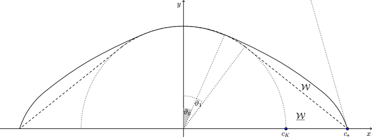
Figure 1: The sets $\mathcal{W}$ (solid line) and $\underline{\mathcal{W}}$ (dashed line) in the case $D>2d$.

The inclusion $\mathcal{W}\supset\underline{\mathcal{W}}$ yields the following estimates on $\mathcal{W}$:

$$\vartheta_{0}<\vartheta_{1}:=\arcsin\frac{c_{K}}{c_{*}},\qquad\forall\vartheta\geq\vartheta_{1},\quad w_{*}(\vartheta)>\frac{c_{K}\,c_{*}}{c_{K}\sin\vartheta+\sqrt{c_{*}^{2}-c_{K}^{2}}\cos\vartheta}.$$

Consider now $w_{*}$ and $c_{*}$ as functions of $D$, with the other parameters frozen. We know from [9] that $c_{*}\to\infty$ as $D\to\infty$. Hence, the above inequalities yield

$$\lim_{D\to\infty}\vartheta_{0}=\lim_{D\to\infty}\vartheta_{1}=0,\qquad\forall\vartheta>0,\quad\liminf_{D\to\infty}w_{*}(\vartheta)\geq\frac{c_{K}}{\cos\vartheta}.$$

Since $w_{*}(\vartheta)\leq c_{K}/\cos\vartheta$, as it is readily seen by comparison with the tangent line $y=c_{K}$, we have the following

Proposition 2.2.

As functions of $D$, the quantities $\vartheta_{0}$ and $w_{*}$ satisfy

$$\lim_{D\to\infty}\vartheta_{0}=0,\qquad\forall\vartheta\in[-\pi/2,\pi/2],\quad\lim_{D\to\infty}w_{*}(\vartheta)=\frac{c_{K}}{\cos\vartheta}.$$

That is, as $D\nearrow\infty$, the set $\mathcal{W}$ increases to fill up the whole strip $\mathbb{R}\times[0,c_{K})$.

Let us give an extension of Theorem 2.1. In [10], we further investigated the effects of transport and reaction on the road. This results in the two additional terms $q\partial_{x}u$ and $g(u)$ in the first equation of (1). We were able to extend the results of [9] under a concavity assumption on $f$ and $g$. The additional assumption on $f$ is not required if $g$ is a pure mortality term, i.e., $g(u)=-\rho u$ with $\rho\geq 0$. This is the most relevant case from the point of view of the applications to population dynamics. The system with transport and pure mortality on the road reads

$$\begin{cases}\partial_{t}u-D\partial_{xx}u+q\partial_{x}u=\nu\!\left.\!\hskip 1.0ptv\right|_{y=0}-\mu u-\rho u,&x\in\mathbb{R},\ t>0\\ \partial_{t}v-d\Delta v=f(v),&(x,y)\in\Omega,\ t>0\\ -d\partial_{y}\!\left.\!\hskip 1.0ptv\right|_{y=0}=\mu u-\nu\!\left.\!\hskip 1.0ptv\right|_{y=0},&x\in\mathbb{R},\ t>0,\end{cases}$$ (5)

with $q\in\mathbb{R}$ and $\rho\geq 0$. The first difference with (1) is that $(\nu/\mu,1)$ is no longer a solution if $\rho\neq 0$. However, we showed in [10] that (5) admits a unique positive, bounded, stationary solution $(U_{S},V_{S})$, with $U_{S}$ constant and $V_{S}$ depending only on $y$ and such that $V_{S}\to 1$ as $y\to+\infty$. We then derived the existence of the asymptotic speed of spreading (to $(U_{S},V_{S})$) in the direction of the line. This is not symmetric if $q\neq 0$. There are indeed two asymptotic speeds of spreading $c_{*}^{\pm}$, in the directions $\pm(1,0)$ respectively. They satisfy $c_{*}^{\pm}\geq c_{K}$, with strict inequality if and only if

$$\frac{D}{d}>2+\frac{\rho}{f^{\prime}(0)}\mp\frac{q}{\sqrt{df^{\prime}(0)}}.$$ (6)

The method developed in the present paper to prove Theorem 2.1 can be adapted to the case of system (5). The details on how this is achieved are given in Section 7 below. In this framework, the notion of the asymptotic expansion shape is modified by replacing $1$ with $V_{S}(y)$ in (4).

Theorem 2.3.

For system (5), the following properties hold true:

1. (Spreading). There exists an asymptotic expansion shape $\mathcal{W}$.

2. (Expansion shape). The set $\mathcal{W}$ is convex and it is of the form

   $$\mathcal{W}=\{r(\sin\vartheta,\cos\vartheta)\ :\ -\pi/2\leq\vartheta\leq\pi/2,\ \ 0\leq r\leq w_{*}(\vartheta)\},$$

   with $w_{*}\in C^{1}([-\pi/2,\pi/2])$ such that

   $$w_{*}=c_{K}\ \text{ in }[\vartheta_{-},\vartheta_{+}],\qquad w_{*}^{\prime}<0\ \text{ in }[-\pi/2,\vartheta_{-}),\qquad w_{*}^{\prime}>0\ \text{ in }(\vartheta_{+},\pi/2],$$

   for some critical angles $-\pi/2\leq\vartheta_{-}<0<\vartheta_{+}\leq\pi/2$.

3. (Directions with enhanced speed). If (6) does not hold then $\vartheta_{\pm}=\pm\pi/2$. Otherwise, if (6) holds, $\vartheta_{\pm}\neq\pm\pi/2$.

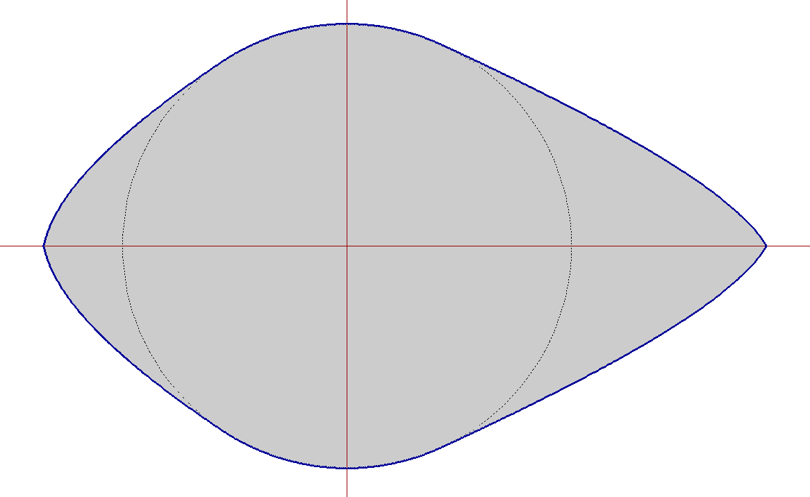
Figure 2: The asymptotic expansion shape in the presence of a transport term towards right on the road ($q>0$).

2.2 Discussion and comments

Let us first comment on how the spreading velocity in the direction $\xi=(\sin\vartheta,\cos\vartheta)$ is sought for. It will be the least $c>0$ such that the linearisation of (1) around 0 admits solutions of the form

$$(U(x,t),V(x,y,t))=(e^{-(\alpha,\beta)\cdot((x,0)-ct\xi)},\gamma e^{-(\alpha,\beta)\cdot((x,y)-ct\xi)}),$$

with $\alpha,\beta\in\mathbb{R}$, $\gamma>0$. Let us point out that $V$ is not exactly a planar wave in the direction $\xi$, for the simple reason that its level sets are not hyperplanes orthogonal to $\xi$, but to $(\alpha,\beta)$. We will find that, when $D>2d$ and $\vartheta$ is larger than a critical angle $\vartheta_{0}$, the vector $(\alpha,\beta)$ associated with the least $c$ is not parallel to $\xi$. This is the reason why the velocity $w_{*}(\vartheta)$ looks different from the classical Freidlin-Gärtner formula [14], that we recall here: for a scalar equation of the form

$$u_{t}-\Delta u+b(x)\cdot\nabla u=\mu(x)u-u^{2},$$ (7)

with $\mu>0$, $\mu$ and $b$ 1-periodic, the spreading velocity in the direction $\xi$ is given by

$$w_{*}(\xi)=\inf_{\xi\cdot\xi^{\prime}>0}\frac{c_{*}(\xi)}{\xi\cdot\xi^{\prime}}$$ (8)

where $c_{*}(\xi)$ is the least $c$ such that the linearisation of (7) around 0:

$$u_{t}-\Delta u+b(x)\cdot\nabla u=\mu(x)u,$$ (9)

admits solutions of the form

$$\phi(x)e^{\lambda(x\cdot\xi-ct)},\ \ \ \ \ \phi>0,\ \hbox{1-periodic.}$$

The optimal assumption for $\mu$ is not, by the way, $\mu>0$. A more general assumption is $\lambda_{1}^{per}(-\Delta-\mu(x))<0$, where $\lambda_{1}^{per}$ denotes the first periodic eigenvalue. In any case, (8) gives the formula

$$\forall\xi,\xi^{\prime}\in\mathbb{R}^{N}\backslash\{0\},\quad c_{*}(\xi)\geq w_{*}(\xi)\xi\cdot\xi^{\prime}.$$

We will see in Section 6 (Lemma 6.1 below) that a similar, but different, formula holds in our case, namely,

$$\forall\vartheta\in[\vartheta_{0},\pi/2],\ \tilde{\vartheta}\in[0,\pi/2],\quad w_{*}(\tilde{\vartheta})\leq\frac{\cos(\vartheta-\varphi_{*}(\vartheta))}{\cos(\tilde{\vartheta}-\varphi_{*}(\vartheta))}\,w_{*}(\vartheta).$$

It will, in fact, be derived as a consequence of the expression of the spreading velocity.

Several proofs of the Freidlin-Gärtner formula have been given, besides that of [14]. See Evans-Souganidis [12] for a viscosity solutions/singular perturbations approach, Weinberger [17] for an abstract monotone system proof; Berestycki-Hamel-Nadin [4] for a PDE proof. See also [5] for equivalent formulae and estimates of the spreading speed in periodic media, as well as [8] for one-dimensional general media. Many of these results are explained, and developped, in [3].

Let us now discuss the shape of the set ${\mathcal{W}}$ in Theorem 2.1, and how it compares to $\underline{\mathcal{W}}$. The latter has a very natural interpretation as the reachable set from the origin in time $1$ by moving with speed $c_{*}$ on the road and $c_{K}$ in the field. Indeed, considering trajectories obtained by moving on the road until time $\lambda\in[0,1]$ and then on a straight line in the field for the remaining time $1-\lambda$, one finds that the reachable set is the convex hull of the union of the segment $[-c_{*},c_{*}]\times\{0\}$ and the half-disc $\overline{B}_{c_{K}}\cap\overline{\Omega}$, that is, $\underline{\mathcal{W}}$.

Another way to obtain the set $\underline{\mathcal{W}}$ is the following: consider a set-valued map $t\mapsto U_{t}\in\overline{\Omega}$ and impose that the trace of $U_{t}$ expands at speed $c_{*}$ on the $x$-axis, and that the rest evolves by asking that the normal velocity of its boundary equals $c_{K}$. In PDE terms, $U_{t}=\{(x,y)\ :\phi(x,y,t)\geq 1\}$, where $\phi$ solves the eikonal equation

$$\begin{cases}\phi_{t}-c_{K}|\nabla\phi|=0&t>0,(x,y)\in\Omega\\ \phi(x,0,t)={\mathbbm{1}}_{[-c_{*}t,c_{*}t]}(x)&t>0,x\in\mathbb{R}\end{cases}$$

So, the family of sets $(U_{t})_{t>0}$ is simply obtained by applying the Huygens principle with the segment $[-c_{*}t,c_{*}t]$ on the road as a source. In other words, $t\underline{\mathcal{W}}=U_{t}$ and it evolves with normal velocity $c_{K}$. Notice that imposing that a family of sets $(tA)_{t>0}$ evolves with normal velocity $c_{K}$ forces the curvature of $A$ to be either $1/c_{K}$ or $0$, i.e., $A$ is locally either a disc of radius $c_{K}$ or a half-plane. It would have been tempting to think that ${\mathcal{W}}$ coincides with $\underline{\mathcal{W}}$, just as in the singular perturbation approach to front propagation in parabolic equations or systems - see Evans-Souganidis [12], [13]. The fact that the asymptotic expansion shape is actually larger than this set is remarkable. And, as a matter of fact, we estimate in Proposition 6.4 below the difference between ${\mathcal{W}}$ and $\underline{\mathcal{W}}$ in terms of the normal velocities of their boundaries when magnified by $t$. Namely, we discover that the normal speed of $(t\mathcal{W})_{t>0}$ at a boundary point $t(\sin\vartheta,\cos\vartheta)$, $\vartheta>\vartheta_{0}$, coincides with the normal speed of the level lines of the planar wave for the linearised system which defines $w_{*}(\vartheta)$ - see the next section. This speed is larger than $c_{K}$ because the exponential decay rate of $V$ in the direction orthogonal to its level lines is less than the critical one: $\sqrt{f^{\prime}(0)/d}$. We expect this decay to be approximatively satisfied for large time by the solution of (1) emerging from a compactly supported initial datum. Thus, heuristically, the presence of the road would result in an “unnatural” decay for solutions of the KPP equation with compactly supported initial data, which, in turns, would be the reason why $\mathcal{W}$ does not coincide with the set $\underline{\mathcal{W}}$ following from Huygens’ principle.

3 Planar waves for the linearised system

Consider the linearisation of system (1) around $v=0$:

$$\begin{cases}\partial_{t}u-D\partial_{xx}u=\nu\!\left.\!\hskip 1.0ptv\right|_{y=0}-\mu u&x\in\mathbb{R},\ t>0\\ \partial_{t}v-d\Delta v=f^{\prime}(0)v&(x,y)\in\Omega,\ t>0\\ -d\partial_{y}\!\left.\!\hskip 1.0ptv\right|_{y=0}=\mu u(x,t)-\nu\!\left.\!\hskip 1.0ptv\right|_{y=0}&x\in\mathbb{R},\ t>0.\end{cases}$$ (10)

Take a unit vector $\xi=(\xi_{1},\xi_{2})$, with $\xi_{2}\geq 0$. By symmetry, we restrict to $\xi_{1}\geq 0$. As said above, solutions are sought for in the form

$$(U(x,t),V(x,y,t))=(e^{-(\alpha,\beta)\cdot((x,0)-ct\xi)},\gamma e^{-(\alpha,\beta)\cdot((x,y)-ct\xi)}),$$ (11)

with $c\geq 0$, $\gamma>0$ and $\alpha,\beta\in\mathbb{R}$ (not necessarily positive). This leads to the system

$$\begin{cases}c\,\xi\cdot(\alpha,\beta)-D\alpha^{2}=\nu\gamma-\mu\\ c\,\xi\cdot(\alpha,\beta)-d(\alpha^{2}+\beta^{2})=f^{\prime}(0)\\ d\gamma\beta=\mu-\nu\gamma.\end{cases}$$

The third equation yields $\gamma=\mu/(\nu+d\beta)$ and then $\beta>-\nu/d$. Setting $\chi(s):=\mu s/(\nu+s)$, the system on $(\alpha,\beta)$ reads

$$\begin{cases}c\xi_{1}\alpha+c\xi_{2}\beta-D\alpha^{2}=-\chi(d\beta)\\ c\xi_{1}\alpha+c\xi_{2}\beta-d(\alpha^{2}+\beta^{2})=f^{\prime}(0).\end{cases}$$ (12)

The first equation in the unknown $\alpha$ has the roots

$$\alpha_{D}^{\pm}(c,\beta):=\frac{1}{2D}\left(c\xi_{1}\pm\sqrt{(c\xi_{1})^{2}+4D\left(c\xi_{2}\beta+\chi(d\beta)\right)}\right),$$

which are real if and only if $\beta$ is larger than some value $\underline{\beta}(c)\in(-\nu/d,0]$. The set of real solutions $(\beta,\alpha)$ of the first equation in (12) is then $\;\Sigma(c)=\Sigma^{-}(c)\cup\Sigma^{+}(c)$, with

$$\Sigma^{\pm}(c):=\{(\beta,\alpha_{D}^{\pm}(c,\beta))\ :\ \beta\geq\underline{\beta}(c)\}.$$

This is a smooth curve with leftmost point $(\underline{\beta}(c),c\xi_{1}/2D)$. Rewriting the second equation in (12) as $\displaystyle|(\alpha,\beta)-\frac{c}{2d}\xi|^{2}=\frac{c^{2}}{4d^{2}}-\frac{f^{\prime}(0)}{d}$, we see that it has solution if and only if $c\geq c_{K}$, where $c_{K}:=2\sqrt{df^{\prime}(0)}$ is the invasion speed in the field. In the $(\beta,\alpha)$ plane, it represents the circle $\Gamma(c)$ of centre $C(c)$ and radius $r(c)$ given by

$$C(c)=\frac{c}{2d}(\xi_{2},\xi_{1}),\qquad r(c)=\frac{\sqrt{c^{2}-c_{K}^{2}}}{2d}.$$

Let $\mathcal{S}(c)$ denote the closed set bounded from below by $\Sigma^{-}(c)$ and from above by $\Sigma^{+}(c)$ and let $\mathcal{G}(c)$ denote the closed disc with boundary $\Gamma(c)$. Exponential functions of the type (11) are supersolutions of (10) if and only if $(\beta,\alpha)\in\mathcal{S}(c)\cap\mathcal{G}(c)$. Since the centre $C(c)$ belongs to the line $s\mapsto s(\xi_{2},\xi_{1})$ and the closest point of $\Gamma(c)$ to the origin, $P(c):=C(c)-r(c)(\xi_{2},\xi_{1})$, satisfies

$$P^{\prime}(c)\cdot(\xi_{2},\xi_{1})=\frac{1}{2d}-\frac{c}{d\sqrt{c^{2}-c_{K}^{2}}}<0,\qquad\lim_{c\to+\infty}P(c)=0,$$

we find that

$$\forall c^{\prime}\geq c\geq c_{K},\quad\mathcal{G}(c^{\prime})\supset\mathcal{G}(c),\qquad\bigcup_{c\geq c_{K}}\mathcal{G}(c)=\{(\beta,\alpha)\ :\ (\beta,\alpha)\cdot(\xi_{2},\xi_{1})>0\}.$$

On the other hand, $\alpha_{D}^{+}(c,\beta)$ is increasing in $c$ and concave in $\beta$, the latter following from the concavity of $c\xi_{2}\beta+\chi(d\beta)$.

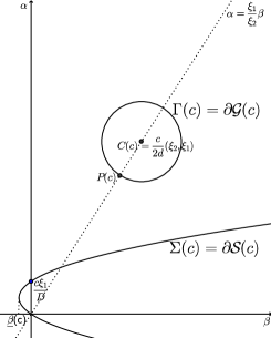
(a) $c<w_{*}$

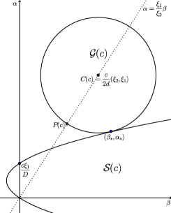
(b) $c=w_{*}$

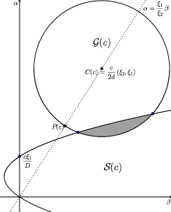
(c) $c>w_{*}$

Figure 3: The case $w_{*}>c_{K}$; supersolutions correspond to the shaded region.

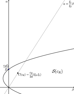
(a) $c=c_{K}$

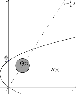
(b) $c>c_{K}$

Figure 4: The case $w_{*}=c_{K}$; supersolutions correspond to the shaded region.

Therefore, there exists $w_{*}\geq c_{K}$, depending on $\xi$, such that

$$\mathcal{S}(c)\cap\mathcal{G}(c)\neq\emptyset\quad\ \Leftrightarrow\ \quad c\geq w_{*},$$

with $\mathcal{S}(w_{*})\cap\mathcal{G}(w_{*})$ consisting in a singleton, denoted by $(\beta_{*},\alpha_{*})$, see Figures 4 and 4. Moreover, $w_{*}=c_{K}$ if and only if $C(c_{K})\in\mathcal{S}(c_{K})$, namely, if and only if $C(c_{K})$ satisfies the first condition in (12) with $=$ replaced by $\geq$ :

$$\frac{c_{K}^{2}}{2d}-\frac{Dc_{K}^{2}}{4d^{2}}\xi_{1}^{2}\geq-\frac{\mu c_{K}\xi_{2}}{2\nu+c_{K}\xi_{2}}.$$

Since $\xi_{1}^{2}=1-\xi_{2}^{2}$, this inequality rewrites

$$2d+D(\xi_{2}^{2}-1)+\frac{4d^{2}\mu\xi_{2}}{2\nu c_{K}+c_{K}^{2}\xi_{2}}\geq 0.$$

The function $\Phi:[0,+\infty)\to\mathbb{R}$ defined by

$$\Phi(s):=2d+D(s^{2}-1)+\frac{4d^{2}\mu s}{2\nu c_{K}+c_{K}^{2}s},$$

is increasing and satisfies $\Phi(0)=2d-D$, $\Phi(1)>0$. As a consequence, $w_{*}=c_{K}$ if and only if either $D\leq 2d$, or $D>2d$ and $\xi_{2}\geq\Phi^{-1}(0)\in(0,1)$. Observe that the sets $\mathcal{S}(c)$ shrink as $D$ increases and therefore $w_{*}$ is a strictly increasing function of $D$ when $w_{*}>c_{K}$.

We now consider the critical speed $w_{*}$ as a function of the angle formed by the vector $\xi$ and the vertical axis. Namely, for $\vartheta\in[-\pi/2,\pi/2]$, we call $w_{*}(\vartheta)$ the quantity defined above associated with $\xi=(\sin\vartheta,\cos\vartheta)$. We further let $(\beta_{*}(\vartheta),\alpha_{*}(\vartheta))$ denote the first contact point $(\beta_{*},\alpha_{*})$. For $\vartheta=\pi/2$, the above construction reduces exactly to the one of [9], thus $w_{*}(\pi/2)$ coincides with the value $c_{*}$ arising in (2). The function $w_{*}$ is even and continuous, as it is immediate to verify. We know that if $D\leq 2d$ then $w_{*}\equiv c_{K}$. Otherwise, if $D>2d$, $w_{*}(\vartheta)>c_{K}$ if and only if $\vartheta>\vartheta_{0}$, where

$$\vartheta_{0}:=\arccos(\Phi^{-1}(0)).$$ (13)

Notice that $\vartheta_{0}$ is a decreasing function of $D$. We finally define

$$\mathcal{W}:=\{r(\sin\vartheta,\cos\vartheta)\ :\ -\pi/2\leq\vartheta\leq\pi/2,\ \ 0\leq r\leq w_{*}(\vartheta)\}.$$

The object of Sections 4 and 5 is to show that $\mathcal{W}$ is the asymptotic expansion set for (1).

4 Compactly supported subsolutions

This section is dedicated to the construction, for all $\vartheta\in(-\pi/2,\pi/2)$, of compactly supported subsolutions moving in the direction $\xi=(\sin\vartheta,\cos\vartheta)$ with speed less than, but arbitrarily close to, $w_{*}(\vartheta)$. We derive the following

Lemma 4.1.

For all $\vartheta\in(-\pi/2,\pi/2)$ and $\varepsilon>0$, there exist $c>w_{*}(\vartheta)-\varepsilon$ and a pair $(\underline{u},\underline{v})$ of nonnegative functions with the following properties: $\!\left.\!\hskip 1.0pt\underline{u}\right|_{t=0}$ and $\!\left.\!\hskip 1.0pt\underline{v}\right|_{t=0}$ are compactly supported,

$$\exists(\hat{x},\hat{y})\in\overline{\Omega},\quad\forall t\geq 0,\quad\underline{v}(\hat{x}+ct\sin\vartheta,\hat{y}+ct\cos\vartheta,t)=\underline{v}(\hat{x},\hat{y},0)>0,$$ (14)

and $\kappa(\underline{u},\underline{v})$ is a generalised subsolution of (1) for all $\kappa\in(0,1]$.

By symmetry, it is sufficient to prove the lemma for $\vartheta\geq 0$. The case $\vartheta=\pi/2$ was treated in [9]. If $\vartheta\in[0,\vartheta_{0}]$ then $w_{*}(\vartheta)=c_{K}$ and the construction is standard, as we will see in Section 4.2. In Section 4.3 we treat the remaining cases by exploiting the analysis of planar waves performed in the previous section. We will proceed as follows:

1. We first give a definition of generalised subsolutions adapted to our context.

2. For $c\in(0,w_{*}(\vartheta))$ close enough to $w_{*}(\vartheta)$, we apply Rouché’s theorem to prove the existence of a complex exponential solution $(U,V)$ of the linearised system, which moves in the direction $\xi=(\sin\vartheta,\cos\vartheta)$ with speed $c$. We actually work on a perturbed system in order to get strict subsolutions of the nonlinear one.

3. The connected components of the positivity set of $u:={\mathrm{Re}}\,U$ are bounded intervals and those of $v:={\mathrm{Re}}\,V$ are infinite strips. In order to truncate those strips, we consider the reflection $v^{L}$ of $v$ with respect to the line $(x,y)\cdot\xi^{\perp}=L>0$. We then define the pair $(\underline{u},\underline{v})$ by setting $(\underline{u},\underline{v})=(u,v-v^{L})$ in a connected component of the positivity sets of $u$ and $v-v^{L}$, $(0,0)$ outside.

4. The function $\underline{v}$ is automatically a generalised subsolution of the equation in the field. We show that, choosing $L$ large enough, $(\underline{u},\underline{v})$ is a generalised subsolution of the equations on the road too.

4.1 Sub/supersolutions

In the sequel, we will need to compare the solution of the Cauchy problem with a pair $(\underline{u},\underline{v})$ which is a subsolution inside some regions, vanishes on their boundaries, and is truncated to 0 outside. In the case of a single equation, such type of functions are generalised subsolutions, in the sense that they satisfy the comparison principle with supersolutions. This kind of properties has the flavour of those presented in [7]. In the case of a system, this property may not hold because, roughly speaking, one could truncate one component in a region where it is needed for the others to be subsolutions. This is why we need a different notion of generalised subsolution.

We consider pairs $(\underline{u},\underline{v})$ such that $\underline{u}$ is the maximum of subsolutions of the first equation in (1) with $v=\underline{v}$, while $\underline{v}$ is the maximum of subsolutions of the second equation and of the last equation with $u=\underline{u}$. More precisely:

Definition 4.2.

A pair $(\underline{u},\underline{v})$ is a generalised subsolution of (1) if $\underline{u}$, $\underline{v}$ are continuous and satisfy the following properties:

1. for any $x\in\mathbb{R}$, $t>0$, there is a function $u$ such that $u\leq\underline{u}$ in a neighbourhood of $(x,t)$ and, at $(x,t)$ (in the classical sense),

   $$u=\underline{u},\qquad\partial_{t}u-D\partial_{xx}u+\mu u\leq\nu\!\left.\!\hskip 1.0pt\underline{v}\right|_{y=0};$$

2. for any $(x,y)\in\overline{\Omega}$, $t>0$, there is a function $v$ such that $v\leq\underline{v}$ in a neighbourhood of $(x,y,t)$ and, at $(x,y,t)$,

   $$v=\underline{v},\qquad\partial_{t}v-d\Delta v\leq f(v)\ \text{ if }y>0,\quad-d\partial_{y}v+\nu v\leq\mu\underline{u}\ \text{\ if }y=0.$$

Although this will not be needed in the paper, we may define generalised supersolutions in analogous way, by replacing “$\leq$” with “$\geq$” everywhere in Definition 4.2. This notion is stronger than that of viscosity solution (see, e.g., [11]). Nevertheless, it recovers: (i) classical subsolutions, (ii) maxima of classical subsolutions and (iii) generalised subsolutions in the sense of [9]. From now on, generalised sub and supersolutions are understood in the sense of Definition 4.2. The comparison principle reads:

Proposition 4.3.

Let $(\underline{u},\underline{v})$ and $(\overline{u},\overline{v})$ be respectively a generalised subsolution bounded from above and a generalised supersolution bounded from below of (1) such that $(\underline{u},\underline{v})$ is below $(\overline{u},\overline{v})$ at time $t=0$. Then $(\underline{u},\underline{v})$ is below $(\overline{u},\overline{v})$ for all $t>0$.

The proof is similar to the one of Proposition 3.3 in [9], even if the notion of sub and supersolution is slightly more general here. It is included here in Appendix Appendix: the generalised comparison principle for the sake of completeness.

4.2 The case $\vartheta\leq\vartheta_{0}$

Let $\lambda(R)$ and $\varphi$ be the principal eigenvalue and eigenfunction of the operator $-d\Delta-c(\sin\vartheta,\cos\vartheta)\cdot\nabla$ in the two dimensional ball $B_{R}$, with Dirichlet boundary condition. This operator can be reduced to a self-adjoint one by multiplying the functions times $e^{(\sin\vartheta,\cos\vartheta)\cdot(x,y)c/2d}$. One then finds that $(\lambda(R)-c^{2}/4d)/d$ is equal to the principal eigenvalue of $-\Delta$ in $B_{R}$. Whence, for $0<c<w_{*}(\vartheta)=c_{K}$,

$$\lim_{R\to\infty}\lambda(R)=\frac{c^{2}}{4d}<f^{\prime}(0).$$

There is then $R>0$ such that $f(s)\geq\lambda(R)s$ for $s>0$ small enough, and therefore we can normalise the principal eigenfunction $\varphi$ in such a way that

$$\forall\kappa\in[0,1],\quad-d\Delta(\kappa\varphi)-c(\sin\vartheta,\cos\vartheta)\cdot\nabla(\kappa\varphi)\leq f(\kappa\varphi)\quad\text{in }B_{R}.$$

It follows that the pair $(\underline{u},\underline{v})$ defined by $\underline{u}\equiv 0$,

$$\underline{v}(x,y,t)=\begin{cases}\varphi(x-ct\sin\vartheta,y-R-ct\cos\vartheta)&\text{if }(x,y-R)-ct(\sin\vartheta,\cos\vartheta)\in B_{R}\\ 0&\text{otherwise}\end{cases}$$

satisfies the properties stated in Lemma 4.1.

4.3 The case $\vartheta>\vartheta_{0}$

Suppose now that $D>2d$ and consider $\vartheta\in(\vartheta_{0},\pi/2)$. Call

$$\xi:=(\sin\vartheta,\cos\vartheta),\qquad\xi^{\perp}:=(-\cos\vartheta,\sin\vartheta),$$

and, to ease notation, $w_{*}=w_{*}(\vartheta)$, $\alpha_{*}=\alpha_{*}(\vartheta)$, $\beta_{*}=\beta_{*}(\vartheta)$.

4.3.1 Complex exponential solutions for the penalised system

We start with the following

Lemma 4.4.

For $c\in(0,w_{*})$ close enough to $w_{*}$, (10) admits an exponential solution $(U,V)$ of the type (11) with $\alpha,\beta,\gamma\in\mathbb{C}\backslash\mathbb{R}$ satisfying

$${\mathrm{Re}}\,\alpha,{\mathrm{Re}}\,\beta>0,\qquad 0<\frac{{\mathrm{Im}}\,\alpha}{{\mathrm{Im}}\,\beta}<\frac{{\mathrm{Re}}\,\alpha}{{\mathrm{Re}}\,\beta}<\frac{\xi_{1}}{\xi_{2}}.$$ (15)

Proof.

For $c<w_{*}$, problem (10) does not admit exponential solutions of the type (11), with $\alpha,\beta,\gamma\in\mathbb{R}$. However, if $w_{*}-c$ is small enough, applying the Rouché theorem to the distance between $\Gamma$ and $\Sigma$ as a function of $\beta$, one obtains an exponential solution $(U,V)$ with $\alpha,\beta,\gamma\in\mathbb{C}$, depending on $c$, and satisfying

$$\alpha=\alpha_{r}+i\alpha_{i},\qquad\beta=\beta_{r}+i\beta_{i},\qquad\gamma=\frac{\mu}{\nu+d\beta},$$

$$\beta_{r}=\beta_{*}+O(w_{*}-c),\qquad 0\neq\beta_{i}=O(\sqrt{w_{*}-c}).$$

See the proof of Lemma 6.1 in [9] for the details. Writing separately the real and complex terms of the second equation of the system (12) satisfied by $\alpha,\beta$, we get

$$\begin{cases}c\xi\cdot(\alpha_{r},\beta_{r})-d(\alpha_{r}^{2}-\alpha_{i}^{2}+\beta_{r}^{2}-\beta_{i}^{2})=f^{\prime}(0)\\ c\xi\cdot(\alpha_{i},\beta_{i})-2d(\alpha_{r}\alpha_{i}+\beta_{r}\beta_{i})=0.\end{cases}$$ (16)

The first equation of (16) yields

$$c\xi_{1}\alpha_{r}-d(\alpha_{r}^{2}-\alpha_{i}^{2})=f^{\prime}(0)-[c\xi_{2}\beta_{*}-d\beta_{*}^{2}]+o(1)=c\xi_{1}\alpha_{*}-d\alpha_{*}^{2}+o(1),\quad\text{as }c\to w_{*}.$$

It follows that

$$\liminf_{c\to w_{*}^{-}}(\alpha_{r}-\frac{c}{2d}\xi_{1})^{2}\geq\liminf_{c\to w_{*}^{-}}(\alpha_{*}-\frac{c}{2d}\xi_{1})^{2}.$$

In particular, $\alpha_{r}$ stays away from $\frac{c}{2d}\xi_{1}$ as $c\to w_{*}^{-}$. Rewriting the second equation of (16) as $(\frac{c}{2d}\xi_{1}-\alpha_{r})\alpha_{i}=(\beta_{r}-\frac{c}{2d}\xi_{2})\beta_{i}$, we then infer that $\alpha_{i}=O(\sqrt{w_{*}-c})$. Then, since ${\mathrm{Im}}\,\gamma=O(\sqrt{w_{*}-c})$ too, considering the real part of (12), we eventually find that $\alpha_{r}=\alpha_{*}+o(1)$ as $c\to w_{*}^{-}$.

We use again the second equation ofprecisely(16) to derive

$$\lim_{c\to w_{*}^{-}}\frac{\alpha_{i}}{\beta_{i}}=\lim_{c\to w_{*}^{-}}\frac{\beta_{r}-\frac{c}{2d}\xi_{2}}{\frac{c}{2d}\xi_{1}-\alpha_{r}}=\frac{\beta_{*}-\frac{c}{2d}\xi_{2}}{\frac{c}{2d}\xi_{1}-\alpha_{*}}.$$

The latter represents the slope of the tangent line to $\mathcal{G}(w_{*})$ at the point $(\beta_{*},\alpha_{*})$. From the convexity of $\mathcal{S}(w_{*})$ we know that this line intersects the $\alpha$-axis at some $\alpha>c\xi_{1}/D$. It follows in particular that its slope is smaller than the one of the line through $(0,0)$ and $(\beta_{*},\alpha_{*})$. This, in turn, is less than the slope of the line through $(0,0)$ and the centre of $\mathcal{G}(w_{*})$, which is parallel to $(\xi_{2},\xi_{1})$, see Figure 5 (a). We deduce that

$$0<\lim_{c\to w_{*}^{-}}\frac{\alpha_{i}}{\beta_{i}}<\frac{\alpha_{*}}{\beta_{*}}=\lim_{c\to w_{*}^{-}}\frac{\alpha_{r}}{\beta_{r}}<\frac{\xi_{1}}{\xi_{2}}.$$

This concludes the proof. ∎

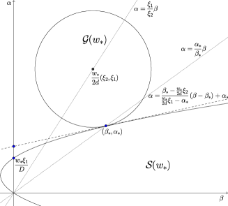
(a) Slope of the tangent line at $(\beta_{*},\alpha_{*})$

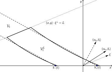
(b) The sets $\mathcal{V}_{t}$ and $\mathcal{V}^{L}_{t}$

Figure 5: Relations between the slopes of $\xi$, $(\alpha_{r},\beta_{r})$ and $(\alpha_{i},\beta_{i})$.

Consider now the penalised system

$$\begin{cases}\partial_{t}u-D\partial_{xx}u=\nu\!\left.\!\hskip 1.0ptv\right|_{y=0}-\mu u-\varepsilon(u+v)&x\in\mathbb{R},\ t>0\\ \partial_{t}v-d\Delta v=(f^{\prime}(0)-\varepsilon)v&(x,y)\in\Omega,\ t>0\\ -d\partial_{y}\!\left.\!\hskip 1.0ptv\right|_{y=0}=\mu u-\nu\!\left.\!\hskip 1.0ptv\right|_{y=0}-\varepsilon(u+v)&x\in\mathbb{R},\ t>0.\end{cases}$$ (17)

A small perturbation $\varepsilon$ does not affect the qualitative results of Section 3 nor that of Lemma 4.4. Thus, for $\varepsilon$ small enough, there exists $w_{*}^{\varepsilon}$ such that (17) admits exponential solutions in the form (11) with $\alpha,\beta,\gamma\in\mathbb{R}$ for $c\geq w_{*}^{\varepsilon}$, and with $\alpha,\beta,\gamma\in\mathbb{C}\backslash\mathbb{R}$ satisfying (15) for $c<w_{*}^{\varepsilon}$ close enough to $w_{*}^{\varepsilon}$. Moreover, $w_{*}^{\varepsilon}\to w_{*}$ as $\varepsilon\to 0$. We are interested in the complex ones. Until the end of Section 4, $(U,V)$ will denote an exponential solution of (17), with $\varepsilon>0$ sufficiently small, $\alpha,\beta,\gamma\in\mathbb{C}\backslash\mathbb{R}$ satisfying (15) and $c<w_{*}^{\varepsilon}$ close to $w_{*}^{\varepsilon}$. Changing the sign to the imaginary part of both $U$ and $V$ we still have a solution. Hence, by (15), it is not restrictive to assume that ${\mathrm{Im}}\,\alpha,{\mathrm{Im}}\,\beta>0$.

We set for short $\alpha_{r}:={\mathrm{Re}}\,\alpha$, $\alpha_{i}:={\mathrm{Im}}\,\alpha$, $\beta_{r}:={\mathrm{Re}}\,\beta$, $\beta_{i}:={\mathrm{Im}}\,\beta$. Since $\gamma^{-1}=(\nu+\varepsilon+d\beta)/(\mu-\varepsilon)$ by the last equation of (17), it follows that ${\mathrm{Arg}}\,(\gamma^{-1})\in(0,\pi/2)$. Resuming, we have:

$$\alpha_{r},\alpha_{i},\beta_{r},\beta_{i}>0,\qquad\frac{\alpha_{i}}{\beta_{i}}<\frac{\alpha_{r}}{\beta_{r}}<\frac{\xi_{1}}{\xi_{2}},\qquad{\mathrm{Arg}}\,(\gamma^{-1})\in(0,\pi/2).$$ (18)

4.3.2 Truncating the exponential solution and the equation in the field

The pair $(u,v)$ defined by

$$u:={\mathrm{Re}}\,U=e^{-(\alpha_{r},\beta_{r})\cdot[(x,0)-ct\xi]}\cos((\alpha_{i},\beta_{i})\cdot[(x,0)-ct\xi]),$$

$$v:={\mathrm{Re}}\,V=|\gamma|e^{-(\alpha_{r},\beta_{r})\cdot[(x,y)-ct\xi]}\cos((\alpha_{i},\beta_{i})\cdot[(x,y)-ct\xi]-{\mathrm{Arg}}\,\gamma),$$

is a real solution of (17). Consider the following connected components of the positivity sets of $u$, $v$ at time $0$:

$$\mathcal{U}=\left(-\frac{\pi}{2\alpha_{i}},\frac{\pi}{2\alpha_{i}}\right),\qquad\mathcal{V}:=\{(x,y)\in\mathbb{R}^{2}\ :\ (\alpha_{i},\beta_{i})\cdot(x,y)\in(-\frac{\pi}{2}+{\mathrm{Arg}}\,\gamma,\frac{\pi}{2}+{\mathrm{Arg}}\,\gamma)\}.$$

As the time $t$ increases, these connected components are shifted, becoming

$$\mathcal{U}_{t}:=\mathcal{U}+ct\{\xi_{1}+\frac{\beta_{i}}{\alpha_{i}}\xi_{2}\},\qquad\mathcal{V}_{t}:=\mathcal{V}+ct\{\xi\}.$$

In order to truncate the sets $\mathcal{V}_{t}$ we consider the reflection with respect to the line $(x,y)\cdot\xi^{\perp}=L$, with $L>0$, where, we recall, $\xi^{\perp}:=(-\cos\vartheta,\sin\vartheta)$. Namely

$$\mathcal{R}^{L}(x,y)=(x,y)+2(L-(x,y)\cdot\xi^{\perp})\xi^{\perp}.$$

We then define

$$V^{L}(x,y,t):=V(\mathcal{R}^{L}(x,y),t),\qquad v^{L}:={\mathrm{Re}}\,V^{L}.$$

The function $v-v^{L}$ vanishes on $(x,y)\cdot\xi^{\perp}=L$ and satisfies the second equation of (17). The quotient $|V^{L}|/|V|$ satisfies

$$\frac{|V^{L}|}{|V|}=\frac{e^{-(\alpha_{r},\beta_{r})\cdot[\mathcal{R}^{L}(x,y)-ct\xi]}}{e^{-(\alpha_{r},\beta_{r})\cdot[(x,y)-ct\xi]}}=e^{-2(\alpha_{r},\beta_{r})\cdot\xi^{\perp}(L-(x,y)\cdot\xi^{\perp})}.$$

Let us call $\sigma:=(\alpha_{r},\beta_{r})\cdot\xi^{\perp}$. It follows from (18) that $\sigma>0$. Hence,

$$\frac{|V^{L}|}{|V|}\leq 1\quad\text{ if }\,(x,y)\cdot\xi^{\perp}\leq L,\qquad\frac{|V^{L}|}{|V|}\leq e^{-\sigma L}\quad\text{ if }\,(x,y)\cdot\xi^{\perp}\leq\frac{L}{2}.$$ (19)

We deduce that, when restricted to the half-plane $\{(x,y)\cdot\xi^{\perp}\leq L/2\}$, a connected component of the set where $(v-v^{L})$ is positive at time $t$, denoted by $\mathcal{V}^{L}_{t}$, converges in Hausdorff distance to $\mathcal{V}_{t}$ as $L\to\infty$, uniformly in $t\geq 0$. We can now define

$$\underline{u}(x,t):=\begin{cases}u(x,t)&\text{if }x\in\mathcal{U}_{t}\\ 0&\text{otherwise},\end{cases}\qquad\underline{v}(x,y,t):=\begin{cases}(v-v^{L})(x,y,t)&\text{if }(x,y)\in\mathcal{V}^{L}_{t}\\ 0&\text{otherwise}.\end{cases}$$

We claim that $\underline{v}$ is bounded. The set $\mathcal{V}^{L}_{t}$ satisfies

$$\mathcal{V}^{L}_{t}\subset\{(x,y)\cdot\xi^{\perp}\leq L\}\cap\{-\pi+{\mathrm{Arg}}\,\gamma\leq(\alpha_{i},\beta_{i})\cdot[(x,y)-ct\xi]\leq\pi+{\mathrm{Arg}}\,\gamma\},$$

as it is seen by noticing that $v=-|V|$ on the boundary of the latter set and $|v^{L}|\leq|V|$ if $(x,y)\cdot\xi^{\perp}\leq L$. Thus

$$\underline{v}\leq 2|\gamma|\sup_{\genfrac{}{}{0.0pt}{}{(x,y)\cdot\xi^{\perp}\leq L}{[(x,y)-ct\xi]\cdot(\alpha_{i},\beta_{i})\geq-\pi+{\mathrm{Arg}}\,\gamma}}e^{-(\alpha_{r},\beta_{r})\cdot[(x,y)-ct\xi]}=2|\gamma|\sup_{\genfrac{}{}{0.0pt}{}{(x,y)\cdot\xi^{\perp}\leq L}{(x,y)\cdot(\alpha_{i},\beta_{i})\geq-\pi+{\mathrm{Arg}}\,\gamma}}e^{-(\alpha_{r},\beta_{r})\cdot(x,y)}.$$

It follows from geometrical considerations that the latter supremum is finite, c.f. Figure 5 (b). Analytically, one sees that it is finite if and only if

$$\{(x,y)\cdot(-\xi^{\perp})\geq 0\}\cap\{(x,y)\cdot(\alpha_{i},\beta_{i})\geq 0\}\subset\{(x,y)\cdot(\alpha_{r},\beta_{r})\geq 0\},$$

which is equivalent to require that $(\alpha_{r},\beta_{r})=\lambda_{1}(-\xi^{\perp})+\lambda_{2}(\alpha_{i},\beta_{i})$ with $\lambda_{1},\lambda_{2}\geq 0$. This property holds true by (18). We therefore have that $(\underline{u},\underline{v})$ is bounded. Furthermore, $\underline{v}$ is a generalized subsolution of the second equation of (17). Since $f(s)\geq(f^{\prime}(0)-\varepsilon)s$ for $s>0$ small enough, we can renormalise $(\underline{u},\underline{v})$ in such a way that $\kappa\underline{v}$ is a generalized subsolution of the second equation of (1) too, for all $\kappa\in[0,1]$. Next, like $v$, $v^{L}$ satisfies $v^{L}((x,y)+ct\xi,t)=v^{L}(x,y,0)$ and thus (14) holds. It only remains to show that $(\underline{u},\underline{v})$ is a generalized subsolution of the equations on the road in the sense of Definition 4.2.

4.3.3 The equations on the road

Let us write

$$\mathcal{U}_{t}=(a_{-}(t),a_{+}(t)),\qquad\mathcal{V}_{t}\cap\{y=0\}=(b_{-}(t),b_{+}(t))\times\{0\}.$$

Since ${\mathrm{Arg}}\,(\gamma^{-1})\in(0,\pi/2)$ by (18), we deduce that

$$b_{-}(t)=a_{-}(t)-\frac{{\mathrm{Arg}}\,(\gamma^{-1})}{\alpha_{i}}<a_{-}(t)<b_{-}(t)+\frac{\pi}{\alpha_{i}}=b_{+}(t)=a_{+}(t)-\frac{{\mathrm{Arg}}\,(\gamma^{-1})}{\alpha_{i}}<a_{+}(t).$$

We further see that

$$\frac{u(b_{\pm}(t)+x,t)}{|U(b_{\pm}(t)+x,t)|}=\pm\sin(-\alpha_{i}x+{\mathrm{Arg}}\,(\gamma^{-1})).$$ (20)

$$\frac{v(b_{\pm}(t)+x,0,t)}{|V(b_{\pm}(t)+x,0,t)|}=\mp\sin(\alpha_{i}x).$$ (21)

For $t\geq 0$ and $(x,0)\in\mathcal{V}_{t}$ we see that

$$x>b_{-}(t)=\frac{1}{\alpha_{i}}(-\frac{\pi}{2}+{\mathrm{Arg}}\,\gamma+ct(\alpha_{i},\beta_{i})\cdot\xi)\geq\frac{1}{\alpha_{i}}(-\frac{\pi}{2}+{\mathrm{Arg}}\,\gamma),$$

whence

$$(x,0)\cdot\xi^{\perp}=-\xi_{2}x<\frac{\xi_{2}}{\alpha_{i}}(\frac{\pi}{2}-{\mathrm{Arg}}\,\gamma).$$

It follows that $\mathcal{V}_{t}\cap\{y=0\}$ is contained in $\{(x,y)\cdot\xi^{\perp}\leq L/4\}$ for $L$ large enough and $t\geq 0$. Thus, the sets $\mathcal{V}^{L}_{t}\cap\{y=0\}$ approach $(b_{-}(t),b_{+}(t))\times\{0\}$ as $L\to+\infty$, uniformly with respect to $t\geq 0$. We consider separately the two equations on the road. Below, the time $t\geq 0$ is fixed and the expressions depending on the $y$-variable are always understood at $y=0$.

The third equation of (1).
The condition involving the third equation of (1) in Definition 4.2 is trivially satisfied if $\underline{v}=0$. Otherwise, if $\underline{v}>0$, then $(x,0)\in\mathcal{V}^{L}_{t}$ and there holds

$$-d\partial_{y}\underline{v}+\nu\underline{v}\leq\mu u-\varepsilon(u+v)+h|V^{L}|,$$

for some $h>0$ only depending on $\alpha,\beta,\xi^{\perp}$. For $L$ large enough, $\mathcal{V}^{L}_{t}\cap\{y=0\}$ is contained in $\{(x,y)\cdot\xi^{\perp}\leq L/2\}$ and then (19) yields

$$-d\partial_{y}\underline{v}+\nu\underline{v}\leq\mu u-\varepsilon(u+v)+h|V|e^{-\sigma L}.$$ (22)

By (20), there exists $k,\delta_{0}>0$ only depending on $\alpha_{i}$ and ${\mathrm{Arg}}\,(\gamma^{-1})$ such that, for $\delta\in(0,\delta_{0})$,

$$\frac{u(x,t)}{|U(x,t)|}<-k\quad\text{if }|x-b_{-}(t)|<\delta,\qquad\frac{u(x,t)}{|U(x,t)|}>k\quad\text{if }|x-b_{+}(t)|<\delta.$$ (23)

Our aim is to show that, for $\delta$ small and $L$ large enough independent of $t$, $(\underline{u},\underline{v})$ is a generalised subsolution of the last equation of (1) for $x\in[b_{-}(t)-\delta,b_{+}(t)+\delta]$. Thus, up to increasing $L$ in such a way that $\mathcal{V}^{L}_{t}\cap\{y=0\}\subset(b_{-}(t)-\delta,b_{+}(t)+\delta)\times\{0\}$ for all $t\geq 0$, it is a generalised subsolution of that equation everywhere.

We first focus on a neighbourhood of $b_{+}$, where $\underline{u}=u$. From (22), using (21), (23) and recalling that $|V|=|\gamma||U|$, we obtain, for $|x-b_{+}(t)|<\delta$,

$$\begin{split}-d\partial_{y}\underline{v}+\nu\underline{v}-\mu\underline{u}&\leq-\varepsilon(u+v)+h|V|e^{-\sigma L}\\ &<[-\varepsilon(k-|\gamma|\alpha_{i}\delta)+h|\gamma|e^{-\sigma L}]|U|.\end{split}$$

Choosing then $\delta\leq k/(2|\gamma|\alpha_{i})$ yields

$$-d\partial_{y}\underline{v}+\nu\underline{v}-\mu\underline{u}<\left(-\frac{\varepsilon k}{2}+h|\gamma|e^{-\sigma L}\right)|U|.$$

We eventually infer that, for $L$ large enough independent of $t$, $(\underline{u},\underline{v})$ is a generalised subsolution of the last equation of (1) in the $\delta$ neighbourhood of $b_{+}(t)$. Consider now points such that $|x-b_{-}(t)|<\delta$, where $\underline{u}=0$. By (22) we get

$$\begin{split}-d\partial_{y}\underline{v}+\nu\underline{v}-\mu\underline{u}&\leq(\mu-\varepsilon)u-\varepsilon v+h|V|e^{-\sigma L}\\ &<[-(\mu-\varepsilon)k+\varepsilon|\gamma|\alpha_{i}\delta+h|\gamma|e^{-\sigma L}]|U|,\end{split}$$

provided that $\varepsilon<\mu$. Taking $\varepsilon<\mu/2$ we end up with the same inequality as in the case $|x-b_{+}(t)|<\delta$ treated above. It remains the case $x\in[b_{-}(t)+\delta,b_{+}(t)-\delta]$. There we have that $v\geq k^{\prime}|V|$, for some $k^{\prime}>0$ only depending on $\alpha_{i}$, $\delta$. Consequently, using the fact that $\underline{u}=\max(u,0)$, we obtain

$$\begin{split}-d\partial_{y}\underline{v}+\nu\underline{v}&\leq(\mu-\varepsilon)u-\varepsilon v+h|V|e^{-\sigma L}\\ &\leq\mu\underline{u}-(\varepsilon k^{\prime}-he^{-\sigma L})|V|.\end{split}$$

We get again a subsolution for $L$ large enough.

The second equation of (1).
The non-trivial case is $x\in\mathcal{U}_{t}=(a_{-}(t),a_{+}(t))$, where

$$\partial_{t}\underline{u}+\mu\underline{u}-\nu\underline{v}=(\nu-\varepsilon)v-\varepsilon u-\nu\underline{v}.$$

If $x\in[b_{+}(t),a_{+}(t))$ then $\partial_{t}\underline{u}+\mu\underline{u}-\nu\underline{v}\leq 0$, provided that $\varepsilon\leq\nu$. As before, let $k,\delta_{0}>0$ be such that (23) holds for $\delta\in(0,\delta_{0})$. Using (21) and the equality $|V|=|\gamma||U|$ we get, if $|x-b_{+}(t)|<\delta$,

$$\partial_{t}\underline{u}+\mu\underline{u}-\nu\underline{v}\leq[|\nu-\varepsilon||\gamma|\alpha_{i}\delta-\varepsilon k]|U|,$$

which is negative for $\delta$ small, independent of $t$. Consider the remaining case $x\in(a_{-}(t),b_{+}(t)-\delta]$. There, from one hand $v\geq k^{\prime}|V|$ with $k^{\prime}$ only depending on $\alpha_{i},\gamma,\delta$, from the other, by (19), $v^{L}\leq|V|e^{-\sigma L}$ provided that $L$ is large enough in such a way that $-a_{-}(t)\cos\vartheta\leq L/2$. Hence,

$$\partial_{t}\underline{u}+\mu\underline{u}-\nu\underline{v}=\nu v^{L}-\varepsilon v-\varepsilon u\leq(\nu e^{-\sigma L}-\varepsilon k^{\prime})|V|.$$

We eventually infer that, for $L$ large enough independent of $t$, $(\underline{u},\underline{v})$ is a generalised subsolution of the second equation of (1). This concludes the proof of Lemma 4.1.

5 Proof of the spreading property

In this section we show that the set $\mathcal{W}$ defined in Section 3 is indeed the asymptotic expansion shape of the system (1). This proves Theorem 2.1 part (i). Moreover, by the definition of the critical angle $\vartheta_{0}$, part (iii) also follows.

We show separately that solutions spread at most and at least with the velocity set $\mathcal{W}$, c.f. (3) and (4) respectively. The upper bound (3) follows by comparison with the planar waves of Section 3. The proof of (4) is more involved. It combines the convergence result close to the road given by [9] with the existence of compactly supported subsolutions provided by Lemma 4.1. Then one concludes using a standard Liouville-type result for strictly positive solutions.

Throughout this section, $(u,v)$ denotes a solution of (1) with an initial datum $(u_{0},v_{0})\not\equiv(0,0)$ compactly supported. As already mentioned in the introduction, the well-posedness of the Cauchy problem is proved in [9].

5.1 The upper bound

Proof of (3).

We prove (3) showing that, for any $\varepsilon>0$, there exists $T>0$ such that the following holds:

$$\forall\vartheta\in[-\pi/2,\pi/2],\ c\geq w_{*}(\vartheta)+\varepsilon,\ t\geq T,\quad v(ct\sin\vartheta,ct\cos\vartheta,t)<\varepsilon.$$

By symmetry, we can restrict ourselves to $\vartheta\in[0,\pi/2]$. Let $R>0$ be such that

$${\mathrm{supp}}\,u_{0}\subset[-R,R],\qquad{\mathrm{supp}}\,v_{0}\subset\overline{B}_{R}.$$

For $\vartheta\in[-\pi/2,\pi/2]$, let $(U_{\vartheta},V_{\vartheta})$ be the planar wave for the linearised system (10) defined by (11) with $\xi=(\sin\vartheta,\cos\vartheta)$, $c=w_{*}(\vartheta)$, $\alpha=\alpha_{*}(\vartheta)$, $\beta=\beta_{*}(\vartheta)$ and $\gamma=\mu/(\nu+d\beta_{*}(\vartheta))$. It is straightforward to check that the functions $\alpha_{*}$ and $\beta_{*}$ are continuous, hence bounded. Since for $\vartheta\in[0,\pi/2]$ it holds that

$$\forall(x,y)\in\overline{B}_{R},\quad U_{\vartheta}(x,0)\geq e^{-|R|\alpha_{*}(\vartheta)},\quad V_{\vartheta}(x,y,0)\geq\frac{\mu}{\nu+d\beta_{*}(\vartheta)}e^{-|R|(\alpha_{*}(\vartheta),\beta_{*}(\vartheta))},$$

there exists $\kappa>0$, independent of $\vartheta$, such that all the $\kappa(U_{\vartheta},V_{\vartheta})$ are above $(u,v)$ at time $0$. The pairs $\kappa(U_{\vartheta},V_{\vartheta})$ are still supersolutions of (10), and then of (1) because, by the KPP hypothesis, $f^{\prime}(0)\kappa V_{\vartheta}\geq f(\kappa V_{\vartheta})$. The comparison principle then yields that, for $\vartheta\in[0,\pi/2]$ and $t\geq 0$, $\kappa V_{\vartheta}\geq v$, whence, in particular,

$$\forall c\geq 0,\quad v(ct\sin\vartheta,ct\cos\vartheta,t)\leq\frac{\kappa\mu}{\nu+d\beta_{*}(\vartheta)}e^{-(c-w_{*}(\vartheta))t(\alpha_{*}(\vartheta),\beta_{*}(\vartheta))\cdot(\sin\vartheta,\cos\vartheta)}.$$

Notice now that the functions $\alpha_{*}$ and $\beta_{*}$ are strictly positive, excepted at $0$ where $\alpha_{*}=0$, $\beta_{*}\neq 0$, and at $\pi/2$ where $\alpha_{*}\neq 0$, $\beta_{*}=0$ if $D\leq 2d$. It follows that $(\alpha_{*}(\vartheta),\beta_{*}(\vartheta))\cdot(\sin\vartheta,\cos\vartheta)$ is positive on $[0,\pi/2]$, thus it has a positive minimum by continuity. The result then follows. ∎

5.2 The lower bound

Proof of (4).

We first show that $v$ is bounded from below away from $0$ in some suitable expanding sets. This allows us to conclude by means of a standard Liouville-type result for entire solutions with positive infimum.

Step 1. For $\varepsilon\in(0,c_{K})$ and $\vartheta\in[-\pi/2,\pi/2]$, there exist $(\hat{x},\hat{y})\in\overline{\Omega}$ and an open set $A$ in the relative topology of $\overline{\Omega}$ such that

$$A\supset\{r(\sin\vartheta,\cos\vartheta)\ :\ 0\leq r\leq w_{*}(\vartheta)-\varepsilon\},\qquad\inf_{\genfrac{}{}{0.0pt}{}{t\geq 1}{(x,y)\in tA}}v(\hat{x}+x,\hat{y}+y,t)>0.$$

Consider the case $\vartheta\neq\pm\pi/2$. Let $(\underline{u},\underline{v})$ be a generalised subsolution given by Lemma 4.1, with $c>w_{*}(\vartheta)-\varepsilon>0$, and set

$$\delta:=\frac{c-w_{*}(\vartheta)+\varepsilon}{2c}\,\in(0,1/2).$$

Even if it means multiplying $\underline{u}$, $\underline{v}$ by a small factor $\kappa>0$, we can assume that $\sup\,\!\left.\!\hskip 1.0pt\underline{u}\right|_{t=0}<\nu/\mu$, $\sup\,\!\left.\!\hskip 1.0pt\underline{v}\right|_{t=0}<1$. We now make use of the spreading result from [9], summarized here by (2). Recalling that the $c_{*}$ there coincides with $w_{*}(\pi/2)$, the second limit implies the existence of $\tau>0$ such that, for $\lambda\in(\delta,1]$ and $|c^{\prime}|<w_{*}(\pi/2)-\varepsilon/2$, the following holds true:

$$\forall(x,y)\in\overline{\Omega},\ t\geq\tau,\quad v(x+c^{\prime}\lambda t,y,\lambda t)>\underline{v}(x,y,0),\quad u(x+c^{\prime}\lambda t,\lambda t)>\underline{u}(x,0).$$

Then, by comparison, $v(x+c^{\prime}\lambda t,y,\lambda t+s)\geq\underline{v}(x,y,s)$ for $t\geq\tau$ and $s\geq 0$, from which, taking $s=(1-\lambda)t$ and $(x,y)=(\hat{x},\hat{y})+c(1-\lambda)t(\sin\vartheta,\cos\vartheta)$, where $(\hat{x},\hat{y})$ is such that (14) holds, we get

$$v(\hat{x}+[c(1-\lambda)\sin\vartheta+c^{\prime}\lambda]t,\hat{y}+[c(1-\lambda)\cos\vartheta]t,t)>\underline{v}(\hat{x},\hat{y},0)>0.$$

Namely,

$$\inf_{\genfrac{}{}{0.0pt}{}{t\geq\tau}{(x,y)\in tA}}v(\hat{x}+x,\hat{y}+y,t)>0,$$

where $A$ is the following set:

$$A=\{(c(1-\lambda)\sin\vartheta+c^{\prime}\lambda,c(1-\lambda)\cos\vartheta)\ :\ \delta<\lambda\leq 1,\ |c^{\prime}|<w_{*}(\pi/2)-\varepsilon/2\},$$

which is open in the relative topology of $\overline{\Omega}$. By the choice of $\delta$, restricting to the values $c^{\prime}=0$ and $2\delta\leq\lambda\leq 1$ in the expression of $A$ we recover the segment $\{r(\sin\vartheta,\cos\vartheta)\ :\ 0\leq r\leq w_{*}(\vartheta)-\varepsilon\}$. While, restricting to $\lambda=1$ and $|c^{\prime}|\leq w_{*}(\pi/2)-\varepsilon$, we obtain $[-w_{*}(\pi/2)+\varepsilon,w_{*}(\pi/2)-\varepsilon]\times\{0\}$, which is the sought segment in the case $\vartheta=\pm\pi/2$. The proof of the step 1 is thereby complete, because the minimum of $v$ on compact subsets of $\overline{\Omega}\times[1,\tau]$ is positive by the strong comparison principle with $(0,0)$.

Step 2. Conclusion.
Fix $\varepsilon\in(0,c_{K})$. Let $((x_{n},y_{n}))_{n\in\mathbb{N}}$ be a sequence in $\overline{\Omega}$ and $(t_{n})_{n\in\mathbb{N}}$ a sequence in $\mathbb{R}_{+}$ such that

$$\lim_{n\to\infty}t_{n}=+\infty,\qquad\forall n\in\mathbb{N},\quad{\mathrm{dist}}\left(\frac{1}{t_{n}}(x_{n},y_{n}),\overline{\Omega}\backslash\mathcal{W}\right)>\varepsilon.$$

By the boundedness of $v$ it follows that $(v(x_{n},y_{n},t_{n}))_{n\in\mathbb{N}}$ converges up to subsequences. In order to prove (4) we need to show that the limits of all converging subsequences are equal to 1. Let us still call $(v(x_{n},y_{n},t_{n}))_{n\in\mathbb{N}}$ one of such subsequences and set

$$m:=\lim_{n\to\infty}v(x_{n},y_{n},t_{n}).$$

If $(y_{n})_{n\in\mathbb{N}}$ admits a bounded subsequence $(y_{n_{k}})_{k\in\mathbb{N}}$ then, since

$$\varepsilon<{\mathrm{dist}}\left(\frac{1}{t_{n_{k}}}(x_{n_{k}},y_{n_{k}}),\overline{\Omega}\backslash\mathcal{W}\right)\leq{\mathrm{dist}}\left(\frac{x_{n_{k}}}{t_{n_{k}}},\mathbb{R}\backslash[-w_{*}(\pi/2),w_{*}(\pi/2)]\right)+\frac{y_{n_{k}}}{t_{n_{k}}},$$

we derive $|x_{n_{k}}|\leq(w_{*}(\pi/2)-\varepsilon/2)t_{n_{k}}$ for $k$ large enough. It then follows from (2) that $m=1$ in this case. Consider now the case where $(y_{n})_{n\in\mathbb{N}}$ diverges. Let us write $1/t_{n}(x_{n},y_{n})=r_{n}(\sin\vartheta_{n},\cos\vartheta_{n})$, with $|\vartheta_{n}|\leq\pi/2$ and $0\leq r_{n}\leq w_{*}(\vartheta_{n})-\varepsilon$, and call $\vartheta$, $r$ the limit of (a subsequence of) $(\vartheta_{n})_{n\in\mathbb{N}}$, $(r_{n})_{n\in\mathbb{N}}$ respectively. The continuity of $w_{*}$ yields $0\leq r\leq w_{*}(\vartheta)-\varepsilon$. Consider the sequence of functions $(v_{n})_{n\in\mathbb{N}}$ defined by

$$v_{n}(x,y,t):=v(x+x_{n},y+y_{n},t+t_{n}).$$

For $n$ large enough, the $v_{n}$ are defined in any given $K\subset\subset\mathbb{R}^{2}\times\mathbb{R}$ and, by interior parabolic estimates (see, e.g., [16]) they are uniformly bounded in $C^{2,\delta}(K)$ and $C^{1,\delta}(K)$ with respect to the space and time variables respectively, for some $\delta\in(0,1)$. Hence, $(v_{n})_{n\in\mathbb{N}}$ converges (up to subsequences) locally uniformly to a solution $v_{\infty}$ of

$$\partial_{t}v_{\infty}-d\Delta v_{\infty}=f(v_{\infty}),\quad(x,y)\in\mathbb{R}^{2},\ t\in\mathbb{R}.$$ (24)

Moreover, $v_{\infty}(0,0,0)=m$. Consider the point $(\hat{x},\hat{y})$ and the set $A$ given by the step 1, associated with $\varepsilon$ and $\vartheta$. For $(x,y)\in\mathbb{R}^{2}$ and $t\in\mathbb{R}$, we see that

$$\lim_{n\to\infty}\frac{1}{t+t_{n}}(x+x_{n}-\hat{x},y+y_{n}-\hat{y})=r(\sin\vartheta,\cos\vartheta)\in A.$$

Thus, for $n$ large enough, since $y+y_{n}-\hat{y}>0$ and $A$ is open in $\overline{\Omega}$, we have that $(x+x_{n}-\hat{x},y+y_{n}-\hat{y})\in(t+t_{n})A$, whence $v_{n}(x,y,t)\geq h>0$, with $h$ independent of $(x,y,t)$. It follows that $v_{\infty}\geq h$ in all $\mathbb{R}^{2}\times\mathbb{R}$. Since $f>0$ in $(0,1)$ and $f<0$ in $(1,+\infty)$, it is straightforward to see by comparison with solutions of the ODE $z^{\prime}=f(z)$ in $\mathbb{R}$, that the unique bounded solution of (24) which is bounded from below away from $0$ is $v_{\infty}\equiv 1$. As a consequence, $m=v_{\infty}(0,0,0)=1$, which concludes the proof of (4). ∎

6 Further properties of the function $w_{*}$

We now study the function $w_{*}:[-\pi/2,\pi/2]\to\mathbb{R}_{+}$ defined in Section 3. This will complete the proof of Theorem 2.1 part (ii). Since $w_{*}$ is even, we restrict ourselves to $[0,\pi/2]$. If $D\leq 2d$ then $w_{*}\equiv c_{K}$. Thus, throughout this section, we assume that $D>2d$. We recall that $(\beta_{*}(\vartheta),\alpha_{*}(\vartheta))$ is the unique intersection point between the sets $\mathcal{S}(w_{*}(\vartheta))$ and $\mathcal{G}(w_{*}(\vartheta))$ associated with $\xi=(\sin\vartheta,\cos\vartheta)$.

We start with the following observation.

Lemma 6.1.

The function $w_{*}$ satisfies

$$\forall\vartheta\in[\vartheta_{0},\pi/2],\ \tilde{\vartheta}\in[0,\pi/2],\quad w_{*}(\tilde{\vartheta})\leq\frac{\cos(\vartheta-\varphi_{*}(\vartheta))}{\cos(\tilde{\vartheta}-\varphi_{*}(\vartheta))}\,w_{*}(\vartheta),$$

where $\varphi_{*}(\vartheta)=\arctan\alpha_{*}(\vartheta)/\beta_{*}(\vartheta)$.

Proof.

Take $\vartheta,\tilde{\vartheta}$ as in the statement of the lemma. The pair $(U,V)$ defined by (11), with $\xi=(\sin\vartheta,\cos\vartheta)$, $c=w_{*}(\vartheta)$, $\alpha=\alpha_{*}(\vartheta)$, $\beta=\beta_{*}(\vartheta)$ and $\gamma=\mu/(\nu+d\beta_{*}(\vartheta))$, is a solution of (10). We call

$$\tilde{\xi}:=(\sin\tilde{\vartheta},\cos\tilde{\vartheta}),\qquad\tilde{c}:=\frac{(\alpha_{*}(\vartheta),\beta_{*}(\vartheta))\cdot\xi}{(\alpha_{*}(\vartheta),\beta_{*}(\vartheta))\cdot\tilde{\xi}}\,w_{*}(\vartheta),$$

and we rewrite $(U,V)$ in the following way:

$$(U(t,x),V(t,x,y))=(e^{-(\alpha_{*}(\vartheta),\beta_{*}(\vartheta))\cdot((x,0)-\tilde{c}t\tilde{\xi})},\gamma e^{-(\alpha_{*}(\vartheta),\beta_{*}(\vartheta))\cdot((x,y)-\tilde{c}t\tilde{\xi})}).$$

Thus, by the definition of $w_{*}(\tilde{\vartheta})$, we derive

$$w_{*}(\tilde{\vartheta})\leq\tilde{c}=\frac{(\alpha_{*}(\vartheta),\beta_{*}(\vartheta))\cdot\xi}{(\alpha_{*}(\vartheta),\beta_{*}(\vartheta))\cdot\tilde{\xi}}\,w_{*}(\vartheta).$$ (25)

The result then follows. ∎

Proposition 6.2.

The function $w_{*}$ satisfies

$$w_{*}\in C^{1}([0,\pi/2]),\qquad w_{*}=c_{K}\ \text{ in }[0,\vartheta_{0}],\qquad w_{*}^{\prime}>0\ \text{ in }(\vartheta_{0},\pi/2].$$

Proof.

The fact that $w_{*}=c_{K}$ in $[0,\vartheta_{0}]$ is just what defines $\vartheta_{0}$, see Section 3. The smoothness of $w_{*}$ outside the point $\vartheta_{0}$ is an easy consequence of the implicit function theorem. Lemma 6.1 implies that, for fixed $\vartheta\in(\vartheta_{0},\pi/2)$, the smooth function $\tilde{\vartheta}\mapsto\frac{\cos(\vartheta-\varphi_{*}(\vartheta))}{\cos(\tilde{\vartheta}-\varphi_{*}(\vartheta))}\,w_{*}(\vartheta)$ touches $w_{*}$ from above at the point $\vartheta$, whence we derive

$$\forall\vartheta\in(\vartheta_{0},\pi/2),\quad w_{*}^{\prime}(\vartheta)=\tan(\vartheta-\varphi_{*}(\vartheta))w_{*}(\vartheta).$$

In particular, $w_{*}^{\prime}(\pi/2)=w_{*}(\pi/2)\beta_{*}(\pi/2)/\alpha_{*}(\pi/2)>0$. For $\vartheta\in(\vartheta_{0},\pi/2)$, we deduce that $w_{*}^{\prime}(\vartheta)>0$ if and only if $\vartheta>\varphi_{*}(\vartheta)$, which is equivalent to $\tan\vartheta>\alpha_{*}(\vartheta)/\beta_{*}(\vartheta)$. Calling as usual $\xi:=(\sin\vartheta,\cos\vartheta)$, this inequality reads $\xi_{1}/\xi_{2}>\alpha_{*}(\vartheta)/\beta_{*}(\vartheta)$, which holds true by geometrical considerations, as already seen in the proof of Lemma 4.4, see Figure 5 (a). As $\vartheta\to\vartheta_{0}^{+}$, the disc $\mathcal{G}(w_{*}(\vartheta))$ collapses to the point $c_{K}/2d(\cos\vartheta_{0},\sin\vartheta_{0})$, whence $w_{*}(\vartheta)\to c_{K}$, $\varphi_{*}(\vartheta)\to\vartheta_{0}$ and eventually $w_{*}^{\prime}(\vartheta)\to 0$. This shows that $w_{*}^{\prime}$ is continuous at $\vartheta_{0}$ too. ∎

To conclude the proof of Theorem 2.1 part (ii) it remains to show that $\mathcal{W}$ is convex and that

$$\mathcal{W}\supsetneq\underline{\mathcal{W}}:={\mathrm{conv}}\big{(}(\overline{B}_{c_{K}}\cap\overline{\Omega})\cup[-c_{*},c_{*}]\times\{0\}\big{)},$$

where, we recall, $c_{*}=w_{*}(\pi/2)$. Proposition 6.2 implies that $\partial\mathcal{W}$ is of class $C^{1}$, except at the extremal points $(\pm c_{*},0)$. The exterior unit normal to $\mathcal{W}$ at those points is understood as the limit of the normals to points of $\Omega\cap\partial\mathcal{W}$ converging to $(\pm c_{*},0)$.

Proposition 6.3.

The set $\mathcal{W}$ is strictly convex and, for $\vartheta\in(\vartheta_{0},\pi/2]$, its exterior unit normal at the point $w_{*}(\vartheta)(\sin\vartheta,\cos\vartheta)$ is parallel to $(\alpha_{*}(\vartheta),\beta_{*}(\vartheta))$.

In particular, $\mathcal{W}\supsetneq\underline{\mathcal{W}}$.

Proof.

Fix $\vartheta\in[\vartheta_{0},\pi/2]$. For $(x,y)\in\mathcal{W}\cap\{x\geq 0\}$, we write $(x,y)=r(\sin\tilde{\vartheta},\cos\tilde{\vartheta})$ for some $\tilde{\vartheta}\in[0,\pi/2]$ and $0\leq r\leq w_{*}(\tilde{\vartheta})$. Using the inequality given by Lemma 6.1 in the form (25), with $\xi=(\sin\vartheta,\cos\vartheta)$ and $\tilde{\xi}:=(\sin\tilde{\vartheta},\cos\tilde{\vartheta})$, yields

$$\begin{split}(\alpha_{*}(\vartheta),\beta_{*}(\vartheta))\cdot(x,y)&=r(\alpha_{*}(\vartheta),\beta_{*}(\vartheta))\cdot\tilde{\xi}\\ &\leq w_{*}(\tilde{\vartheta})(\alpha_{*}(\vartheta),\beta_{*}(\vartheta))\cdot\tilde{\xi}\leq w_{*}(\vartheta)(\alpha_{*}(\vartheta),\beta_{*}(\vartheta))\cdot\xi,\end{split}$$

and equality holds if and only if $(x,y)=w_{*}(\vartheta)\xi$. This shows that $\mathcal{W}\cap\{x\geq 0\}$ is contained in the half-plane $\{(\alpha_{*}(\vartheta),\beta_{*}(\vartheta))\cdot(x,y)<w_{*}(\vartheta)(\alpha_{*}(\vartheta),\beta_{*}(\vartheta))\cdot(\sin\vartheta,\cos\vartheta)\}$, except for the point $w_{*}(\vartheta)(\sin\vartheta,\cos\vartheta)$ which belongs to its boundary. Then, clearly, the same property holds for the whole $\mathcal{W}$. This shows the convexity of $\mathcal{W}$ and the directions of the normal vectors.

Let us prove the last statement of the proposition. Proposition 6.2 implies that $\mathcal{W}$ contains $\overline{B}_{c_{K}}\cap\overline{\Omega}$, whence, being convex, it contains $\underline{\mathcal{W}}$. We prove that $\mathcal{W}\not\equiv\underline{\mathcal{W}}$ by showing that the (acute) angle $\varphi_{*}$ formed by $\mathcal{W}$ with the $x$-axis is strictly larger than the one formed by $\underline{\mathcal{W}}$, which is $\vartheta_{1}:=\arcsin(c_{K}/c_{*})$. We know from the first part of the proposition that $\varphi_{*}=\arctan(\alpha_{*}/\beta_{*})$, where, for short, $\alpha_{*}:=\alpha_{*}(\pi/2)$ and $\beta_{*}:=\beta_{*}(\pi/2)$. Recall that $(\beta_{*},\alpha_{*})$ is the tangent point between the sets $\mathcal{S}(c_{*})$ and $\mathcal{G}(c_{*})$ associated with $\xi=(1,0)$, defined in Section 3. It then follows from geometrical considerations that $\varphi_{*}>\vartheta_{1}$, see Figure 6. ∎

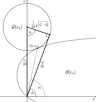
Figure 6: The angles $\varphi_{*}$ and $\vartheta_{1}$.

We deduce from Proposition 6.3 and Figure 4 (b) that, for $\vartheta\in(\vartheta_{0},\pi/2]$, the exterior normal at the point $w_{*}(\vartheta)(\sin\vartheta,\cos\vartheta)$ is steeper than $(\sin\vartheta,\cos\vartheta)$.

Let us finally estimate by how much $\mathcal{W}$ is larger than $\underline{\mathcal{W}}$.

Proposition 6.4.

The family of sets $(t\mathcal{W})_{t>0}$ evolves with normal speed $c_{K}$ in the sector $\{(\sin\vartheta,\cos\vartheta)\ :|\vartheta|\leq\vartheta_{0}\}$ and with normal speed strictly larger than $c_{K}$ in the sectors $\{(\sin\vartheta,\cos\vartheta)\ :\vartheta_{0}<|\vartheta|\leq\pi/2\}$.

Proof.

The assertion for the sector $\{(\sin\vartheta,\cos\vartheta)\ :|\vartheta|\leq\vartheta_{0}\}$ trivially holds because $\mathcal{W}$ coincides with $B_{c_{K}}$ there. Consider $\vartheta\in(\vartheta_{0},\pi/2]$ and set $\xi:=(\sin\vartheta,\cos\vartheta)$. By Proposition 6.3, the exterior unit normal to $\mathcal{W}$ at the point $w_{*}(\vartheta)\xi$ is

$$\mathbf{n}(\vartheta):=\frac{(\alpha_{*}(\vartheta),\beta_{*}(\vartheta))}{|(\alpha_{*}(\vartheta),\beta_{*}(\vartheta))|}.$$

Hence, the speed of expansion of the set $t\mathcal{W}$ at the point $tw_{*}(\vartheta)\xi$ in the normal direction $\mathbf{n}(\vartheta)$ is $c_{\mathbf{n}}(\vartheta):=w_{*}(\vartheta)\xi\cdot\mathbf{n}(\vartheta).$ This is precisely the normal speed of the level lines of the function $V$ defined by (11) with $c=w_{*}(\vartheta)$, $\alpha=\alpha_{*}(\vartheta)$, $\beta=\beta_{*}(\vartheta)$ and $\gamma=\mu/(\nu+d\beta_{*}(\vartheta))$. Indeed, we can rewrite

$$V(x,y,t)=\gamma e^{-|(\alpha_{*}(\vartheta),\beta_{*}(\vartheta))|[(x,y)\cdot\mathbf{n}(\vartheta)-c_{\mathbf{n}}(\vartheta)t]}.$$

Plugging the above expression in the second equation of (10) satisfied by $V$, we get

$$c_{\mathbf{n}}(\vartheta)=\frac{f^{\prime}(0)}{|(\alpha_{*}(\vartheta),\beta_{*}(\vartheta))|}+d|(\alpha_{*}(\vartheta),\beta_{*}(\vartheta))|.$$

The function $\mathbb{R}_{+}\ni\lambda\mapsto f^{\prime}(0)/\lambda+d\lambda$ attains its minimum $c_{K}$ at the unique value $\lambda=\sqrt{f^{\prime}(0)/d}$. Thus, to prove the proposition we need to show that $|(\alpha_{*}(\vartheta),\beta_{*}(\vartheta))|\neq\sqrt{f^{\prime}(0)/d}$. This follows from the geometrical interpretation of the point $P_{*}\equiv(\beta_{*}(\vartheta),\alpha_{*}(\vartheta))$, see Figure 4 (b): the convexity of $\mathcal{S}(c)$ implies that the angle between the segments $\overline{P_{*}\,C(c)}$ and $\overline{P_{*}\,O}$, $O$ denoting the origin, is larger than $\pi/2$, whence, since these segments have length $\sqrt{c^{2}-c_{K}^{2}}/2d$ and $c/2d$ respectively, elementary considerations about the triangle $O\,P_{*}\,C(c)$ show that $|(\alpha_{*}(\vartheta),\beta_{*}(\vartheta))|<c_{K}^{2}/2d=\sqrt{f^{\prime}(0)/d}$. ∎

7 The case with transport and mortality on the road

We now describe how to modify the arguments used for problem (1) in order to treat the case of (5). This is done section by section, keeping the same notation.

Section 3.
We need to consider the values $\xi_{1}\leq 0$ too. The transport and mortality terms affect (12) through the additional term $-q\alpha+\rho$ in the left-hand side of the first equation. This results in the new functions

$$\alpha_{D}^{\pm}(c,\beta)=\frac{1}{2D}\left(c\xi_{1}-q\pm\sqrt{(c\xi_{1}-q)^{2}+4D(c\xi_{2}\beta+\chi(d\beta)+\rho)}\right).$$

One can readily check that $\alpha_{D}^{+}(c,\beta)$ is still increasing in $c$ and concave in $\beta$. It further satisfies the following property, that will be crucial in the sequel: $\alpha_{D}^{+}(c,0)\geq 0$. We can therefore define $w_{*}$ as before. We have that $w_{*}=c_{K}$ if and only if $C(c_{K})\in\mathcal{S}(c_{K})$, which now reads

$$\frac{c_{K}^{2}}{2d}-\frac{Dc_{K}^{2}}{4d^{2}}\xi_{1}^{2}-\frac{qc_{K}}{2d}\xi_{1}+\rho\geq-\frac{\mu c_{K}\xi_{2}}{2\nu+c_{K}\xi_{2}}.$$

This inequality can be rewritten in terms of $\xi_{1}$ as $\Phi(\xi_{1})\geq 0$, with

$$\Phi(s):=2-\frac{D}{d}s^{2}-\frac{2q}{c_{K}}s+\frac{4d\rho}{c_{K}^{2}}+\frac{4d\mu\sqrt{1-s^{2}}}{2\nu c_{K}+c_{K}^{2}\sqrt{1-s^{2}}}.$$

Explicit computation shows that all the above terms are concave in $s$. Hence, since $\Phi(0)>0$ and $\Phi(\pm\infty)=-\infty$, there are two values $s_{-}<0<s_{+}$ such that $w_{*}=c_{K}$ if and only if $\xi_{1}\in[s_{-},s_{+}]$. We have that $|s_{\pm}|<1$ if and only if $\Phi(\pm 1)<0$, which is precisely condition (6). Therefore, writing $w_{*}$ as a function of the angle $\vartheta$, we derive the condition for the enhancement of the speed stated in Theorem 2.3, with $\vartheta_{\pm}=\arcsin s_{\pm}$ if (6) holds, $\vartheta_{\pm}=\pm\pi/2$ otherwise. For $\vartheta=\pm\pi/2$, we recover the asymptotic speeds of spreading $c_{*}^{\pm}$ in the directions $\pm(1,0)$ given by Theorem 1.1 of [10].

Section 4.
The only point one has to check is the argument to derive (15) in the proof of Lemma 4.4. That argument is based on the fact that the slope of the tangent line to $\mathcal{G}(w_{*})$ at the point $(\beta_{*},\alpha_{*})$ is less than $\alpha_{*}/\beta_{*}$, which, in turn, is less than $\xi_{1}/\xi_{2}$. This properties follow exactly as before, from the fact that $\alpha_{D}^{+}$ is concave in $\beta$ and it is nonnegative at $\beta=0$.

Section 5.
The proof of the upper bound (3) works exactly as for Theorem 2.1. In the lower bound (4), the value $1$ is now replaced by the function $V_{S}(y)$. However, since $V_{s}(+\infty)=1$, we can proceed exactly as in Section 5.2, by use of the compactly supported subsolutions and the convergence result close to the road. The latter is now provided by Theorem 1.1 of [10].

The arguments in Section 6 are unaffected by the presence of the additional terms.

Appendix: the generalised comparison principle

Proof of Proposition 4.3.

Following the arguments of the proof of Proposition 3.2 in [9], we start with reducing $(\overline{u},\overline{v})$ to a strict supersolution $(\hat{u},\hat{v})$ which is strictly above $(\underline{u},\underline{v})$ at time $0$ and satisfies

$$\lim_{|x|\to\infty}\hat{u}(x,t)=+\infty,\quad\lim_{|(x,y)|\to\infty}\hat{v}(x,y,t)=+\infty,\quad\text{uniformly w.r.t.\leavevmode\nobreak\ }t\geq 0.$$ (26)

To do this, we first multiply $(\underline{u},\underline{v})$ and $(\overline{u},\overline{v})$ by $e^{-lt}$, where $l$ is the Lipschitz constant of $f$, and we end up with generalised sub and supersolutions (still denoted $(\underline{u},\underline{v})$ and $(\overline{u},\overline{v})$) of the new system

$$\begin{cases}\partial_{t}u-D\partial_{xx}u+(\mu+l)u=\nu\!\left.\!\hskip 1.0ptv\right|_{y=0},&x\in\mathbb{R},\ t>0\\ \partial_{t}v-d\Delta v=h(t,v),&(x,y)\in\Omega,\ t>0\\ -d\partial_{y}\!\left.\!\hskip 1.0ptv\right|_{y=0}+\nu\!\left.\!\hskip 1.0ptv\right|_{y=0}=\mu u,&x\in\mathbb{R},\ t>0,\\ \end{cases}$$ (27)

with $h(t,v):=e^{-lt}f(ve^{lt})-lv$. In such a way we gain the nonincreasing monotonicity in $v$ of the nonlinear term $h$. Next, we introduce a nonnegative smooth function $\chi:\mathbb{R}\to\mathbb{R}$ satisfying

$$\chi=0\ \text{ in }[0,1],\qquad\lim_{r\to+\infty}\chi(r)=+\infty,\qquad|\chi^{\prime\prime}|\leq\delta,$$

where $\delta>0$ will be chosen later. Then, for $\varepsilon>0$, we set

$$\hat{u}(x,t):=\overline{u}(x,t)+\varepsilon(\chi(|x|)+t+1),\qquad\hat{v}(x,y,t):=\overline{v}(x,y,t)+\frac{\mu}{\nu}\varepsilon(\chi(|x|)+\chi(y)+t+1),$$

We claim that $\delta$ can be chosen small enough, independently of $\varepsilon$, in such a way that $(\hat{u},\hat{v})$ is still a generalised supersolution of (27), in the strict sense for the first two equations. Take $\overline{x}\in\mathbb{R}$ and $\overline{t}>0$. By the definition of generalised supersolution, there exists a function $u$ satisfying $u\geq\overline{u}$ in a neighbourhood of $(\overline{x},\overline{t})$ and, at $(\overline{x},\overline{t})$,

$$u=\overline{u},\qquad\partial_{t}u-D\partial_{xx}u+(\mu+l)u\geq\nu\!\left.\!\hskip 1.0pt\overline{v}\right|_{y=0}.$$

The function $\tilde{u}(x,t):=u(x,t)+\varepsilon(\chi(|x|)+t+1)$ satisfies $\tilde{u}\geq\hat{u}$ in a neighbourhood of $(\overline{x},\overline{t})$ and, at $(\overline{x},\overline{t})$,

$$\tilde{u}=\hat{u},\qquad\partial_{t}\tilde{u}-D\partial_{xx}\tilde{u}+(\mu+l)\tilde{u}\geq\nu\!\left.\!\hskip 1.0pt\hat{v}\right|_{y=0}+\varepsilon(1-D\chi^{\prime\prime}(|x|)).$$

Then the desired strict inequality holds provided $\delta<1/D$. For the second equation, we start from a “test function” $v$ at some $(\overline{x},\overline{y})\in\Omega$, $\overline{t}>0$ and we see that $\tilde{v}(x,y,t):=v(x,y,t)+\frac{\mu}{\nu}\varepsilon(\chi(|x|)+\chi(y)+t+1)$ satisfies, at $(\overline{x},\overline{y},\overline{t})$,

$$\partial_{t}\tilde{v}-d\Delta\tilde{v}\geq h(\overline{t},v)+\frac{\mu}{\nu}\varepsilon(1-2d\delta).$$

If $\delta<1/2d$, the right hand side is strictly larger than $h(\overline{t},v)$, which, in turn, is larger than $h(t,\tilde{v})$ by the monotonicity of $h$. The case of the third equation is straightforward. The claim is thereby proved.

The pair $(\hat{u},\hat{v})$ is strictly above $(\underline{u},\underline{v})$ at $t=0$. Assume by contradiction that $(\hat{u},\hat{v})$ is not strictly above $(\underline{u},\underline{v})$ for all time and call

$$T:=\sup\{t\geq 0\ :\ \underline{u}<\hat{u}\text{ in }\mathbb{R}\times[0,t],\ \underline{v}<\hat{v}\text{ in }\overline{\Omega}\times[0,t]\}\,\in[0,+\infty).$$

It follows that $\underline{u}\leq\hat{u}$ in $\mathbb{R}\times[0,T]$, $\underline{v}\leq\hat{v}$ in $\overline{\Omega}\times[0,T]$. Moreover, by (26) and the continuity of the functions we see that $T>0$ and either $\hat{u}-\underline{u}$ or $\hat{v}-\underline{v}$ vanish somewhere at time $T$. Suppose that $(\hat{u}-\underline{u})(x,T)=0$ for some $x\in\mathbb{R}$. We now use the fact that $(\underline{u},\underline{v})$ and $(\hat{u},\hat{v})$ are a subsolution and a strict supersolution respectively of (27), in the generalised sense. There exist $u_{1}$, $u_{2}$ such that $u_{1}\leq\underline{u}\leq\hat{u}\leq u_{2}$ in some cylinder $\mathcal{C}:=B_{\delta}(x)\times(T-\delta,T]$ and, at $(x,T)$, $u_{1}=\underline{u}=\hat{u}=u_{2}$ and

$$\partial_{t}u_{1}-D\partial_{xx}u_{1}+(\mu+l)u_{1}\leq\nu\!\left.\!\hskip 1.0pt\underline{v}\right|_{y=0}\leq\nu\!\left.\!\hskip 1.0pt\hat{v}\right|_{y=0}<\partial_{t}u_{2}-D\partial_{xx}u_{2}+(\mu+l)u_{2}.$$

Since $(x,T)$ is a maximum point for $u_{1}-u_{2}$ in $\mathcal{C}$, we have that, there, $\partial_{t}u_{1}=\partial_{t}u_{2}$ and $\partial_{xx}u_{1}\leq\partial_{xx}u_{2}$. We then get a contradiction with the above strict inequality. Thus, $\min_{\mathbb{R}}(\hat{u}-\underline{u})(\cdot,T)>0$ and there exists $(x,y)\in\overline{\Omega}$ such that $(\hat{v}-\underline{v})(x,y,T)=0$. Using the other two equations of (27), we find $v_{1}$, $v_{2}$ such that $v_{1}\leq\underline{v}\leq\hat{v}\leq v_{2}$ in a cylinder $\mathcal{C}:=B_{\delta}(x,y)\times(T-\delta,T]$ and, at $(x,y,T)$, $v_{1}=\underline{v}=\hat{v}=v_{2}$ and

$$\partial_{t}v_{1}-d\Delta v_{1}\leq h(T,v_{1})=h(T,v_{2})<\partial_{t}v_{2}-d\Delta v_{2}\quad\text{if }y>0,$$

$$-d\partial_{y}v_{1}+\nu v_{1}\leq\mu\underline{u}<\mu\hat{u}\leq-d\partial_{y}v_{2}+\nu v_{2}\quad\text{if }y=0.$$

As before, we get a contradiction with the fact that $v_{1}-v_{2}$ has a maximum in $\mathcal{C}$ at $(x,y,T)$. ∎

References

- [1] Aronson, D.G; Weinberger, H.F. Nonlinear diffusion in population genetics, combustion, and nerve pulse propagation. In Partial differential equations and related topics (Program, Tulane Univ., New Orleans, La., 1974), 446 5–49. Springer, Berlin, 1975.
- [2] Aronson, D. G.; Weinberger, H. F. Multidimensional nonlinear diffusion arising in population genetics. Adv. in Math. 30 (1978), no. 1, 33–76.
- [3] Berestycki, H; Hamel, F. Reaction-diffusion equations and propagation phenomena. Applied Mathematical Sciences, 2014.
- [4] Berestycki, H; Hamel, F.; Nadin, G. Asymptotic spreading in heterogeneous diffusive excitable media. J. Funct. Analysis, 255 (2008), 2146–2189.
- [5] Berestycki, H.; Hamel, F.; Nadirashvili, N. The speed of propagation for KPP type problems. I. Periodic framework. J. Eur. Math. Soc. (JEMS), 7(2005), 173–213.
- [6] Berestycki, H; Hamel, F.; Nadirashvili, N. The speed of propagation for KPP type problems. II. General domains. J. Amer. Math. Soc., 23 (2010), 1–34.
- [7] Berestycki, H.; Lions, P.-L. Some applications of the method of super and subsolutions. in Bifurcation and nonlinear eigenvalue problems (Proc., Session, Univ. Paris XIII, Villetaneuse, 1978), Lecture Notes in Math., vol. 782, pp. 16–41, Springer, Berlin, 1980.
- [8] Berestycki, H.; Nadin, G. Spreading speeds for one-dimensional monostable reaction-diffusion equations. J. Math. Phys., 53 (2012).
- [9] Berestycki, H.; Roquejoffre, J.-M.; Rossi, L. The influence of a line with fast diffusion on Fisher-KPP propagation. J. Math. Biol. 66 (2013), no. 4-5, 743–766.
- [10] Berestycki, H.; Roquejoffre, J.-M.; Rossi, L. Fisher-KPP propagation in the presence of a line: Further effects. Nonlinearity 26 (2013), no. 9, 2623–2640.
- [11] Crandall, M. G.; Ishii, H.; Lions, P.-L. User’s guide to viscosity solutions of second order partial differential equations. Bull. Amer. Math. Soc. (N.S.) 27 (1992), no. 1, 1–67.
- [12] Evans, L. C.; Souganidis, P. E. A PDE approach to certain large deviation problems for systems of parabolic equations. Analyse non linéaire (Perpignan, 1987). Ann. Inst. H. Poincaré Anal. Non Linéaire 6 (1989), suppl., 229–258.
- [13] Evans, L.C; Souganidis, P.E. A PDE approach to geometric optics for certain semilinear parabolic equations. Indiana Univ. Math. J. 38 (1989), 141–172.
- [14] Gartner, J.; Freidlin, M.I. The propagation of concentration waves in periodic and random media. Dokl. Akad. Nauk SSSR, 249 (1979), 521?525.
- [15] Kolmogorov, A. N.; Petrovskiĭ, I. G.; Piskunov, N. S. Étude de l’équation de la diffusion avec croissance de la quantité de matière et son application à un problème biologique. Bull. Univ. Etat. Moscow Ser. Internat. Math. Mec. Sect. A 1 (1937), 1–26.
- [16] Ladyženskaja, O. A.; Solonnikov, V. A.; Ural′ceva, N. N. Linear and quasilinear equations of parabolic type, Translated from the Russian by S. Smith. Translations of Mathematical Monographs, Vol. 23, American Mathematical Society, Providence, R.I., 1967.
- [17] Weinberger, H. F. On spreading speeds and traveling waves for growth and migration models in a periodic habitat. J. Math. Biol. 45 (2002), no. 6, 511–548.
- [18]