Uncertainty Propagation in Elasto-Plastic Material

Abstract

Macroscopically heterogeneous materials, characterised mostly by comparable heterogeneity lengthscale and structural sizes, can no longer be modelled by deterministic approach instead. It is convenient to introduce stochastic approach with uncertain material parameters quantified as random fields and/or random variables. The present contribution is devoted to propagation of these uncertainties in mechanical modelling of inelastic behaviour. In such case the Monte Carlo method is the traditional approach for solving the proposed problem. Nevertheless, convergence rate is relatively slow, thus new methods (e.g. stochastic Galerkin method, stochastic collocation approach, etc.) have been recently developed to offer fast convergence for sufficiently smooth solution in the probability space. Our goal is to accelerate the uncertainty propagation using a polynomial chaos expansion based on stochastic collocation method. The whole concept is demonstrated on a simple numerical example of uniaxial test at a material point where interesting phenomena can be clearly understood.

1 Introduction

Probabilistic or stochastic mechanics deals with mechanical systems, which are either subject to random external influences - a random or uncertain environment, or are themselves uncertain, or both, cf. e.g. the reports [10, 13, 20]. From a mathematical point of view, these systems can be characterised by stochastic ordinary/partial differential equations (SODEs/SPDEs), which can be solved by stochastic finite element method (SFEM). SFEM is an extension of the classical deterministic finite element approach to the stochastic framework i.e. to the solution of stochastic (static and dynamic) problems involving finite elements whose properties are random, see [24]

Nowadays, Monte Carlo (MC) is the most widely used technique in simulating models driven by SODEs/SPDEs. MC simulations require thousands or millions samples because of relatively slow convergence rate, thus the total cost of these numerical evaluations quickly becomes prohibitive. To meet this concern, the surrogate models based on the polynomial chaos expansion (PCE), see [25, 26], were developed as a promising alternative. PC-based surrogates are constructed by different fully-, semi- or non-intrusive methods based on the stochastic Galerkin method [8, 20], stochastic collocation (SC) method [3, 4, 28] or DoE (design of experiments)-based linear regression  [5]. The principal differences among these methods are as follows. Stochastic Galerkin method is purely deterministic (nonsampling method), but leads to solution of large system of equations and needs a complete intrusive modification of the numerical model (and/or existing finite element code) itself. Consequently, suitable robust numerical solver is required. On the other hand, SC method is a sampling method, does not require intrusive modification of a model, but uses a set of model simulations. The computation of PCE coefficients is based on explicit formula and computational effort depends only on the chosen level of accuracy and corresponding number of grid points, see [8, 20, 27]. The linear regression is based again on a set of model simulations performed for a stochastic design of experiments, usually obtained by Latin Hypercube Sampling. The PCE coefficients are then obtained by a regression of model results at the design points, which leads to a solution of a system of equations. A short overview of yet another approaches for solving SODEs/SPDEs is available in [27].

In particular, this paper is focused on the modelling of uncertainties in elasto-plastic material. While numerical studies using MC methods have been presented during several years, the PC-based strategies has emerged only recently,  [1, 2, 21]. The authors mostly extended original work of Ghanem and Spanos [8] to elasto-plasticity problem by approximating spatial varying material properties and model responses using Karhunen-Loève and PCE, respectively. The interested reader may also consult an excellent work on this subject by Rosic [22]. However, all these works concentrate especially on the stochastic Galerkin method and SC method is discussed only marginally. Hence this paper is devoted to the application of SC method and for a sake of simplicity we focus here on uncertainty propagation in elasto-plastic material at a single material point.

The paper is organised as follows: A problem setting is presented in Section 2, followed by description of material model in Section 3 and surrogate model in Section 4. Section 5 then demonstrates the proposed framework on elasto-plasticity problem at material point. The essential findings are summarised in Section 6.

2 Problem setting

This paper is focused on the modelling of uncertainties in properties of elasto-plastic material and investigates the influence of such uncertainties on mechanical behaviour. To fulfill this objective, we introduce a bounded body $D\subset\mathbb{R}^{3}$ (reference configuration) with a piecewise smooth boundary $\partial D$. In particular, the Dirichlet and Neumann boundary conditions are imposed on $\Gamma_{\mathrm{D}}\subset\partial D$ and $\Gamma_{\mathrm{N}}\subset\partial D$, respectively, such that $\partial D=\Gamma_{\mathrm{D}}\cup\Gamma_{\mathrm{N}}$. Moreover, we are interested in the time-dependent behavior of $D$, thus we consider a time interval $[0,T]\subset\mathbb{R}_{+}$. The evolution of the material body $D$ in the geometrically linear regime is expressed as

$$\mathchoice{\displaystyle\boldsymbol{u}}{\textstyle\boldsymbol{u}}{\scriptstyle\boldsymbol{u}}{\scriptscriptstyle\boldsymbol{u}}:D\times[0,T]\longrightarrow\mathbb{R}^{3},$$ (1)

where $\mathchoice{\displaystyle\boldsymbol{u}}{\textstyle\boldsymbol{u}}{\scriptstyle\boldsymbol{u}}{\scriptscriptstyle\boldsymbol{u}}\,\mathrm{[m]}$ is the displacement field. In a quasi-static setting, the linear momentum balance equation is then described by

$$-\,\mathrm{div}\mathchoice{\displaystyle\boldsymbol{\sigma}}{\textstyle\boldsymbol{\sigma}}{\scriptstyle\boldsymbol{\sigma}}{\scriptscriptstyle\boldsymbol{\sigma}}(x,t)=\mathchoice{\displaystyle\boldsymbol{f}}{\textstyle\boldsymbol{f}}{\scriptstyle\boldsymbol{f}}{\scriptscriptstyle\boldsymbol{f}}(x,t),\quad x\in D,\,t\in[0,T]$$ (2)

and corresponding boundary conditions

$$\mathchoice{\displaystyle\boldsymbol{\sigma}}{\textstyle\boldsymbol{\sigma}}{\scriptstyle\boldsymbol{\sigma}}{\scriptscriptstyle\boldsymbol{\sigma}}(x,t)\cdot\mathchoice{\displaystyle\boldsymbol{n}}{\textstyle\boldsymbol{n}}{\scriptstyle\boldsymbol{n}}{\scriptscriptstyle\boldsymbol{n}}(x) = \mathchoice{\displaystyle\boldsymbol{t}}{\textstyle\boldsymbol{t}}{\scriptstyle\boldsymbol{t}}{\scriptscriptstyle\boldsymbol{t}}_{\mathrm{N}}(x,t),\qquad\qquad\qquad\qquad$$ (3)

$$x\in\Gamma_{\mathrm{N}},\,t\in[0,T],$$

$$\mathchoice{\displaystyle\boldsymbol{u}}{\textstyle\boldsymbol{u}}{\scriptstyle\boldsymbol{u}}{\scriptscriptstyle\boldsymbol{u}}(x,t) = \mathchoice{\displaystyle\boldsymbol{u}}{\textstyle\boldsymbol{u}}{\scriptstyle\boldsymbol{u}}{\scriptscriptstyle\boldsymbol{u}}_{\mathrm{D}}(x,t),\qquad\qquad\qquad\qquad$$ (4)

$$x\in\Gamma_{\mathrm{D}},\,t\in[0,T],$$

where $\mathchoice{\displaystyle\boldsymbol{\sigma}}{\textstyle\boldsymbol{\sigma}}{\scriptstyle\boldsymbol{\sigma}}{\scriptscriptstyle\boldsymbol{\sigma}}(x,t)\,\mathrm{[Pa]}$ is the stress tensor, $\mathchoice{\displaystyle\boldsymbol{f}}{\textstyle\boldsymbol{f}}{\scriptstyle\boldsymbol{f}}{\scriptscriptstyle\boldsymbol{f}}(x,t)\,\mathrm{[Nm^{-3}]}$ is the body forces, $\mathchoice{\displaystyle\boldsymbol{n}}{\textstyle\boldsymbol{n}}{\scriptstyle\boldsymbol{n}}{\scriptscriptstyle\boldsymbol{n}}\,\mathrm{[-]}$ is the exterior unit normal, $\mathchoice{\displaystyle\boldsymbol{t}}{\textstyle\boldsymbol{t}}{\scriptstyle\boldsymbol{t}}{\scriptscriptstyle\boldsymbol{t}}_{\mathrm{N}}(x,t)\,\mathrm{[Pa]}$ is the prescribed surface tension and $\mathchoice{\displaystyle\boldsymbol{u}}{\textstyle\boldsymbol{u}}{\scriptstyle\boldsymbol{u}}{\scriptscriptstyle\boldsymbol{u}}_{\mathrm{D}}(x,t)\,\mathrm{[m]}$ is the prescribed displacement.

Consider now a system involving material variability. If the input parameter is defined as a random variable and/or field, the system would be governed by a set of SPDEs and the corresponding responses would also be random vectors of nodal displacements, see  [15, 17]. Let $(\Omega,\mathscr{S},\mathbb{P})$ be a complete probability space with $\Omega$ the set of the elementary events $\omega$, $\mathbb{P}$ the probability measure and $\mathscr{S}$ an $\sigma$-algebra on the set $\Omega$. Following previous definitions of the evolution of the material body $D$ (Eq. 1), we are now concerned with the mapping in the stochastic setting:

$$\mathchoice{\displaystyle\boldsymbol{u}}{\textstyle\boldsymbol{u}}{\scriptstyle\boldsymbol{u}}{\scriptscriptstyle\boldsymbol{u}}:D\times[0,T]\times\Omega\longrightarrow\mathbb{R}^{3}.$$ (5)

Consequently, the linear momentum balance equation is then given by

$$-\,\mathrm{div}\mathchoice{\displaystyle\boldsymbol{\sigma}}{\textstyle\boldsymbol{\sigma}}{\scriptstyle\boldsymbol{\sigma}}{\scriptscriptstyle\boldsymbol{\sigma}}(x,t,\omega)=\mathchoice{\displaystyle\boldsymbol{f}}{\textstyle\boldsymbol{f}}{\scriptstyle\boldsymbol{f}}{\scriptscriptstyle\boldsymbol{f}}(x,t,\omega),\qquad\qquad\qquad\qquad$$

$$\qquad\qquad\qquad x\in D,\,t\in[0,T],\,\omega\in\Omega$$ (6)

and corresponding boundary conditions

$$\mathchoice{\displaystyle\boldsymbol{\sigma}}{\textstyle\boldsymbol{\sigma}}{\scriptstyle\boldsymbol{\sigma}}{\scriptscriptstyle\boldsymbol{\sigma}}(x,t,\omega)\cdot\mathchoice{\displaystyle\boldsymbol{n}}{\textstyle\boldsymbol{n}}{\scriptstyle\boldsymbol{n}}{\scriptscriptstyle\boldsymbol{n}}(x) = \mathchoice{\displaystyle\boldsymbol{t}}{\textstyle\boldsymbol{t}}{\scriptstyle\boldsymbol{t}}{\scriptscriptstyle\boldsymbol{t}}_{\mathrm{N}}(x,t,\omega),\qquad\qquad\qquad\qquad$$ (7)

$$x\in\Gamma_{\mathrm{N}},\,t\in[0,T],\,\omega\in\Omega,$$

$$\mathchoice{\displaystyle\boldsymbol{u}}{\textstyle\boldsymbol{u}}{\scriptstyle\boldsymbol{u}}{\scriptscriptstyle\boldsymbol{u}}(x,t,\omega) = \mathchoice{\displaystyle\boldsymbol{u}}{\textstyle\boldsymbol{u}}{\scriptstyle\boldsymbol{u}}{\scriptscriptstyle\boldsymbol{u}}_{\mathrm{D}}(x,t,\omega),\qquad\qquad\qquad\qquad$$ (8)

$$x\in\Gamma_{\mathrm{D}},\,t\in[0,T],\,\omega\in\Omega.$$

In order to solve this stochastic partial differential equation and obtain the approximate responses of the system, MC method is usually used. The effort of performing MC simulations is high, and hence strategies based on the surrogate models have been developed to accelerate the SPDEs solution. In particular, we employ the polynomial expansion and collocation method described concisely in Section  4.

3 Material Model

In order to demonstrate a performance of the SC method, we briefly introduce the mathematical formulation of the deterministic elasto-plastic behaviour. The basic equations of flow plasticity theory start from the decomposition of strain rate vector $\dot{\mathchoice{\displaystyle\boldsymbol{\varepsilon}}{\textstyle\boldsymbol{\varepsilon}}{\scriptstyle\boldsymbol{\varepsilon}}{\scriptscriptstyle\boldsymbol{\varepsilon}}}\,\mathrm{[-]}$ in an elastic (reversible) part $\dot{\mathchoice{\displaystyle\boldsymbol{\varepsilon}}{\textstyle\boldsymbol{\varepsilon}}{\scriptstyle\boldsymbol{\varepsilon}}{\scriptscriptstyle\boldsymbol{\varepsilon}}}\,\mathrm{[-]}$ and a plastic (irreversible) part $\dot{\mathchoice{\displaystyle\boldsymbol{\varepsilon}}{\textstyle\boldsymbol{\varepsilon}}{\scriptstyle\boldsymbol{\varepsilon}}{\scriptscriptstyle\boldsymbol{\varepsilon}}}_{\mathrm{p}}\,\mathrm{[-]}$, see  [9, 18],

$$\dot{\mathchoice{\displaystyle\boldsymbol{\varepsilon}}{\textstyle\boldsymbol{\varepsilon}}{\scriptstyle\boldsymbol{\varepsilon}}{\scriptscriptstyle\boldsymbol{\varepsilon}}}=\dot{\mathchoice{\displaystyle\boldsymbol{\varepsilon}}{\textstyle\boldsymbol{\varepsilon}}{\scriptstyle\boldsymbol{\varepsilon}}{\scriptscriptstyle\boldsymbol{\varepsilon}}}_{\mathrm{e}}+\dot{\mathchoice{\displaystyle\boldsymbol{\varepsilon}}{\textstyle\boldsymbol{\varepsilon}}{\scriptstyle\boldsymbol{\varepsilon}}{\scriptscriptstyle\boldsymbol{\varepsilon}}}_{\mathrm{p}}.$$ (9)

The elastic strain rate is related to the stress rate according to constitutive relation for an isotropic elastic material as

$$\dot{\mathchoice{\displaystyle\boldsymbol{\sigma}}{\textstyle\boldsymbol{\sigma}}{\scriptstyle\boldsymbol{\sigma}}{\scriptscriptstyle\boldsymbol{\sigma}}}=\mathchoice{\displaystyle\boldsymbol{D}}{\textstyle\boldsymbol{D}}{\scriptstyle\boldsymbol{D}}{\scriptscriptstyle\boldsymbol{D}}_{\mathrm{e}}:\dot{\mathchoice{\displaystyle\boldsymbol{\varepsilon}}{\textstyle\boldsymbol{\varepsilon}}{\scriptstyle\boldsymbol{\varepsilon}}{\scriptscriptstyle\boldsymbol{\varepsilon}}_{\mathrm{e}}},$$ (10)

where $\mathchoice{\displaystyle\boldsymbol{D}}{\textstyle\boldsymbol{D}}{\scriptstyle\boldsymbol{D}}{\scriptscriptstyle\boldsymbol{D}}_{\mathrm{e}}\,\mathrm{[Pa]}$ is the elastic material stiffness matrix. The associated flow rule is usually defined using the plastic multiplier and the plastic potential, which is in this case equal to a particular yield criterion, as

$$\dot{\mathchoice{\displaystyle\boldsymbol{\varepsilon}}{\textstyle\boldsymbol{\varepsilon}}{\scriptstyle\boldsymbol{\varepsilon}}{\scriptscriptstyle\boldsymbol{\varepsilon}}}_{\mathrm{p}}=\dot{\lambda}\frac{\partial f(\mathchoice{\displaystyle\boldsymbol{\sigma}}{\textstyle\boldsymbol{\sigma}}{\scriptstyle\boldsymbol{\sigma}}{\scriptscriptstyle\boldsymbol{\sigma}},\sigma_{\mathrm{y}})}{\partial\mathchoice{\displaystyle\boldsymbol{\sigma}}{\textstyle\boldsymbol{\sigma}}{\scriptstyle\boldsymbol{\sigma}}{\scriptscriptstyle\boldsymbol{\sigma}}}.$$ (11)

It remains to characterise loading/unloading conditions established in standard Karush–Kuhn–Tucker form as

$$f\leq 0,\quad\dot{\lambda}\geq 0,\quad\dot{\lambda}f=0.$$ (12)

Just for the sake of completeness, we introduce the simplest and most useful yield condition formulated by Maxwell–Huber–Hencky–von Mises, often called $J_{2}$-plasticity, see [6]. Here, the yield criterion is expressed as

$$f(\mathchoice{\displaystyle\boldsymbol{\sigma}}{\textstyle\boldsymbol{\sigma}}{\scriptstyle\boldsymbol{\sigma}}{\scriptscriptstyle\boldsymbol{\sigma}},\sigma_{\mathrm{y}})=\sqrt{J_{2}}-\frac{\sigma_{\mathrm{y}}(\kappa)}{\sqrt{3}},$$ (13)

where $J_{2}\,\mathrm{[Pa^{2}]}$ is the second invariant of the deviatoric stress, $\sigma_{\mathrm{y}}(\kappa)\,\mathrm{[Pa]}$ is the tensile yield strength. Here, we assume a bilinear form of strain hardening plasticity described by an evolution of the tensile yield strength as a function of a hardening parameter $\kappa$ as

$$\sigma_{\mathrm{y}}(\kappa)=\sigma_{\mathrm{y}}(\varepsilon_{\mathrm{p}}^{\mathrm{eq}})=\sigma_{\mathrm{y,0}}+H\varepsilon_{\mathrm{p}}^{\mathrm{eq}},$$ (14)

where $H\,\mathrm{[Pa]}$ is the hardening parameter, $\sigma_{\mathrm{y,0}}\,\mathrm{[Pa]}$ is the initial yield strength and $\varepsilon_{\mathrm{p}}^{\mathrm{eq}}\,\mathrm{[-]}$ is the equivalent plastic strain calculated as $\varepsilon_{\mathrm{p}}^{\mathrm{eq}}=\sqrt{(\frac{2}{3}\,\mathchoice{\displaystyle\boldsymbol{\varepsilon}}{\textstyle\boldsymbol{\varepsilon}}{\scriptstyle\boldsymbol{\varepsilon}}{\scriptscriptstyle\boldsymbol{\varepsilon}}_{\mathrm{p}}:\mathchoice{\displaystyle\boldsymbol{\varepsilon}}{\textstyle\boldsymbol{\varepsilon}}{\scriptstyle\boldsymbol{\varepsilon}}{\scriptscriptstyle\boldsymbol{\varepsilon}}_{\mathrm{p}})}$. The most popular approach for integrating the constitutive equations of isotropic hardening $J_{2}$-plasticity is the radial return method proposed by Krieg and Krieg, see [14]. The stability and efficiency of the algorithms and also details of the algorithmic formulation may be found in [6, 12].

4 Surrogate model

The construction of a surrogate of the computational model can be used for a significant acceleration of each sample evaluation. Here we use the SC method [3, 4, 28] to construct the surrogate model based on the PCE.

4.1 Polynomial chaos expansion

In modelling of heterogeneous material, some material parameters are not constants, but can be described as random variables (RVs), namely real-valued random variables $X:\Omega\rightarrow\mathbb{R}$ specified completely by their cumulative distribution functions (CDFs). From a mathematical and computational point of view, it is better to use independent random variables for numerical integration over the probability space $\Omega$, see [15, 20]. Therefore, we introduce set of independent Gaussian random variables $\mathchoice{\displaystyle\boldsymbol{\xi}}{\textstyle\boldsymbol{\xi}}{\scriptstyle\boldsymbol{\xi}}{\scriptscriptstyle\boldsymbol{\xi}}(\omega)=(\xi_{1}(\omega),\dots,\xi_{s}(\omega)])^{\mathrm{T}}$ with zero mean and unit variance, see [20, 26] . According to the Doob-Dynkin lemma [27], the model response $\mathchoice{\displaystyle\boldsymbol{u}}{\textstyle\boldsymbol{u}}{\scriptstyle\boldsymbol{u}}{\scriptscriptstyle\boldsymbol{u}}(\mathchoice{\displaystyle\boldsymbol{\xi}}{\textstyle\boldsymbol{\xi}}{\scriptstyle\boldsymbol{\xi}}{\scriptscriptstyle\boldsymbol{\xi}}(\omega))=\left(\dots,u_{l}(\mathchoice{\displaystyle\boldsymbol{\xi}}{\textstyle\boldsymbol{\xi}}{\scriptstyle\boldsymbol{\xi}}{\scriptscriptstyle\boldsymbol{\xi}}(\omega)),\dots\right)^{\mathrm{T}}$ is a random vector which can be expressed in terms of the same random variables $\mathchoice{\displaystyle\boldsymbol{\xi}}{\textstyle\boldsymbol{\xi}}{\scriptstyle\boldsymbol{\xi}}{\scriptscriptstyle\boldsymbol{\xi}}(\omega)$. Since $\mathchoice{\displaystyle\boldsymbol{\xi}}{\textstyle\boldsymbol{\xi}}{\scriptstyle\boldsymbol{\xi}}{\scriptscriptstyle\boldsymbol{\xi}}(\omega)$ are independent standard Gaussian RVs, Wiener’s PCE based on multivariate Hermite polynomials —orthogonal in the Gaussian measure—$\{H_{\alpha}(\mathchoice{\displaystyle\boldsymbol{\xi}}{\textstyle\boldsymbol{\xi}}{\scriptstyle\boldsymbol{\xi}}{\scriptscriptstyle\boldsymbol{\xi}}(\omega))\}_{\alpha\in\mathcal{J}}$ is the most suitable choice for the approximation $\tilde{\mathchoice{\displaystyle\boldsymbol{u}}{\textstyle\boldsymbol{u}}{\scriptstyle\boldsymbol{u}}{\scriptscriptstyle\boldsymbol{u}}}(\mathchoice{\displaystyle\boldsymbol{\xi}}{\textstyle\boldsymbol{\xi}}{\scriptstyle\boldsymbol{\xi}}{\scriptscriptstyle\boldsymbol{\xi}}(\omega))$ of the model response $\mathchoice{\displaystyle\boldsymbol{u}}{\textstyle\boldsymbol{u}}{\scriptstyle\boldsymbol{u}}{\scriptscriptstyle\boldsymbol{u}}(\mathchoice{\displaystyle\boldsymbol{\xi}}{\textstyle\boldsymbol{\xi}}{\scriptstyle\boldsymbol{\xi}}{\scriptscriptstyle\boldsymbol{\xi}}(\omega))$ [26], and it can be written as

$$\tilde{\mathchoice{\displaystyle\boldsymbol{u}}{\textstyle\boldsymbol{u}}{\scriptstyle\boldsymbol{u}}{\scriptscriptstyle\boldsymbol{u}}}(\mathchoice{\displaystyle\boldsymbol{\xi}}{\textstyle\boldsymbol{\xi}}{\scriptstyle\boldsymbol{\xi}}{\scriptscriptstyle\boldsymbol{\xi}}(\omega))=\sum_{\alpha\in\mathcal{J}}\mathchoice{\displaystyle\boldsymbol{u}}{\textstyle\boldsymbol{u}}{\scriptstyle\boldsymbol{u}}{\scriptscriptstyle\boldsymbol{u}}_{\alpha}H_{\alpha}(\mathchoice{\displaystyle\boldsymbol{\xi}}{\textstyle\boldsymbol{\xi}}{\scriptstyle\boldsymbol{\xi}}{\scriptscriptstyle\boldsymbol{\xi}}(\omega)),$$ (15)

where $\mathchoice{\displaystyle\boldsymbol{u}}{\textstyle\boldsymbol{u}}{\scriptstyle\boldsymbol{u}}{\scriptscriptstyle\boldsymbol{u}}_{\alpha}$ is a vector of PC coefficients and the index set $\mathcal{J}\subset\mathbb{N}_{0}^{(\mathbb{N})}$ is a finite set of non-negative integer sequences with only finitely many non-zero terms, i.e. multi-indices, with cardinality $|\mathcal{J}|=R$.

4.2 Stochastic collocation

As a preamble, it has been proven that for sufficiently smooth solution in the probability space, SC method achieves as fast convergence as stochastic Galerkin method, see [27]. Moreover, utilisation of existing deterministic solvers for repetitive runs and especially no need for numerical model modification are important practical aspects. Such properties make the SC method more preferred alternative to stochastic Galerkin method and MC method for solving SODEs/SPDEs, see [26, 27, 28].

In principle, SC method is based on the approximation of stochastic solution using appropriate multivariate polynomials. According to  [27], the SC method can be seen as a high-order ”deterministic sampling method.” The formulation is based on an explicit expression of the PC coefficients as, see [3, 4, 28]:

$$u_{\alpha,l}=\int_{\Omega}u_{l}(\mathchoice{\displaystyle\boldsymbol{\xi}}{\textstyle\boldsymbol{\xi}}{\scriptstyle\boldsymbol{\xi}}{\scriptscriptstyle\boldsymbol{\xi}})H_{\alpha}(\mathchoice{\displaystyle\boldsymbol{\xi}}{\textstyle\boldsymbol{\xi}}{\scriptstyle\boldsymbol{\xi}}{\scriptscriptstyle\boldsymbol{\xi}})\,\mathrm{d}\mathbb{P}(\mathchoice{\displaystyle\boldsymbol{\xi}}{\textstyle\boldsymbol{\xi}}{\scriptstyle\boldsymbol{\xi}}{\scriptscriptstyle\boldsymbol{\xi}})\,,$$ (16)

which can be solved numerically using an appropriate integration (quadrature) rule on $\mathbb{R}^{s}$. Equation (16) then becomes

$$u_{\alpha,l}=\frac{1}{\gamma_{{}_{\alpha}}}\sum_{j=1}^{i}u_{l}(\mathchoice{\displaystyle\boldsymbol{\xi}}{\textstyle\boldsymbol{\xi}}{\scriptstyle\boldsymbol{\xi}}{\scriptscriptstyle\boldsymbol{\xi}}_{j})H_{\alpha}(\mathchoice{\displaystyle\boldsymbol{\xi}}{\textstyle\boldsymbol{\xi}}{\scriptstyle\boldsymbol{\xi}}{\scriptscriptstyle\boldsymbol{\xi}}_{j})w_{j}\,,$$ (17)

where $\gamma_{{}_{\alpha}}=\mathbb{E}[H_{\alpha}^{2}(\mathchoice{\displaystyle\boldsymbol{\xi}}{\textstyle\boldsymbol{\xi}}{\scriptstyle\boldsymbol{\xi}}{\scriptscriptstyle\boldsymbol{\xi}})]$ are the normalization constants of PC basis, $\mathchoice{\displaystyle\boldsymbol{\xi}}{\textstyle\boldsymbol{\xi}}{\scriptstyle\boldsymbol{\xi}}{\scriptscriptstyle\boldsymbol{\xi}}_{j}$ stands for an integration node, $w_{j}$ is a corresponding weight and $i$ is the number of quadrature points. Once we have obtained accurate PC approximation, following analytical relations replacing exhaustive sampling procedure of PC expansion are used to calculate mean $\mu_{l}$ and standard deviation $\sigma^{\mathrm{STD}}_{l}$

$$\mu_{l}=\mathbb{E}[\tilde{u_{l}}] \approx \int_{\Omega}\left(\sum_{\alpha\leq r}u_{\alpha,l}H_{\alpha}(\mathchoice{\displaystyle\boldsymbol{\xi}}{\textstyle\boldsymbol{\xi}}{\scriptstyle\boldsymbol{\xi}}{\scriptscriptstyle\boldsymbol{\xi}})\right)\,\mathrm{d}\mathbb{P}(\mathchoice{\displaystyle\boldsymbol{\xi}}{\textstyle\boldsymbol{\xi}}{\scriptstyle\boldsymbol{\xi}}{\scriptscriptstyle\boldsymbol{\xi}})=u_{0,l},$$ (18)

$$\sigma^{\mathrm{STD}}_{l}=\sqrt{\mathbb{E}[(\tilde{u}_{l}-\mathbb{E}[\tilde{u}_{l}])^{2}]} \approx \sqrt{\left(\sum_{0<\alpha\leq r}\gamma_{\alpha}\,u_{\alpha,l}^{2}\right)}.$$ (19)

According to Eq. (17), the computational effort of SC method is given by the effort needed for realisation of $i$ deterministic simulations. Particular number of simulations $i$ and their spatial positions follow from choice of a desired accuracy. Here we employ version of the Smolyak quadrature rule, in particular nested Kronrod-Patterson version, see [11]. This methodology produces significantly less collocation points than other quadrature rules, see [28]. For a detailed mathematical formulation and corresponding numerical technique of several sparse quadratures construction, we refer the interested reader to [3, 4, 11, 27]. For an illustration, Kronrod-Patterson sparse grids for two Gaussian random variables and different accuracy levels (number of points) are plotted in Fig. 1.

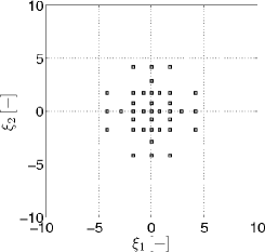
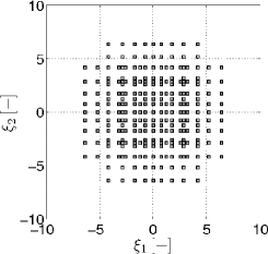
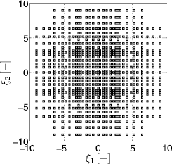
(a)	(b)	(c)

Figure 1: Kronrod-Patterson quadrature rule for two Gaussian random variables and different number of collocation points: (a) $i=37$; (b) $i=261$; (c) $i=921$

5 Example: Plasticity problem at a material point

Symbol	Type of variable	Value	Mean ($\mu_{q}$)	Standard deviation ($\sigma^{\mathrm{STD}}_{q}$)
$E$	lognormal RV	-	$210\cdot 10^{9}$	$21\cdot 10^{9}$
$\nu$	constant	$0.3$	-	-
$\sigma_{\mathrm{y,0}}$	constant	$235\cdot 10^{6}$	-	-
$H$	constant	$2.1\cdot 10^{9}$	-	-

Table 1: Input material parameters of numerical study

So as to demonstrate the described methodology on elasto-plastic problem, we employ a numerical simulation of uniaxial tensile test at a material point. For a sake of clarity, we introduce a simple elasto-plastic model with four material parameters listed in Tab. 1 and we consider only Young’s modulus $E\,\mathrm{[Pa]}$ to be uncertain. With respect to its physical meaning, we describe it by a lognormally distributed RV. Remaining three input parameters, namely Poisson’s ratio $\nu\,\mathrm{[-]}$, initial yield strength $\sigma_{\mathrm{y,0}}\,\mathrm{[Pa]}$ and hardening parameter $H\,\mathrm{[Pa]}$ are assumed to be a constant. The solution of the elasto-plastic problem involves a discretization into $80$ uniform time steps $T$.

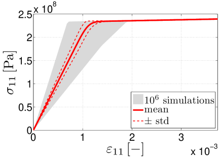
Figure 2: Reference MC simulations corresponding to material parameters in Tab. 1, evolution of $\sigma_{11}\,\mathrm{[Pa]}$ as function of $\varepsilon_{11}\,\mathrm{[-]}$

First of all, we investigate the accuracy of SC-based strategy in predicting mean, standard deviation and $0.01-$quantile of model response $\sigma_{11}\,\mathrm{[Pa]}$. The quality of a PC-based surrogate depends on the number $i$ of collocation points and on the degree of polynomials $p$ used in Eq. (15). In order to assess the accuracy of surrogate models constructed for different number of points $i$ and polynomial degree $p$, we compare the obtained predictions with a reference solution computed by MC method using $10^{6}$ samples, see Fig. 2. To quantify the difference between the resulting predictions of mean $\mu$, standard deviation $\sigma^{\mathrm{STD}}$ and quantile $Q^{0.01}$ of model response $\sigma_{11}\,\mathrm{[Pa]}$, we define following relative error:

$$e(v) = \frac{\|v-v_{\mathrm{MC}}\|_{l^{2}([0,T]\times\Omega)}}{\|v_{\mathrm{MC}}\|_{l^{2}([0,T]\times\Omega)}},$$ (20)

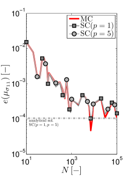
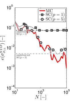
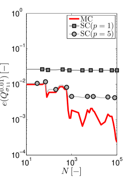
(a)	(b)	(c)
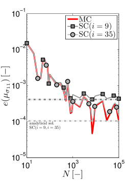
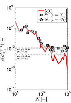
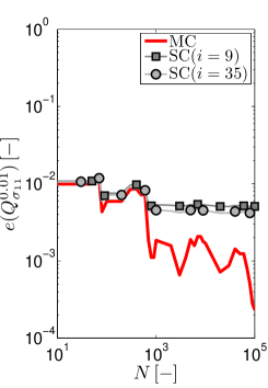
(d)	(e)	(f)

Figure 3: Error analysis of (a) mean $\mu\,\mathrm{[-]}$, (b) standard deviation $\sigma^{\mathrm{STD}}\,\mathrm{[-]}$ and (c) quantile $Q^{0.01}\,\mathrm{[-]}$ for fixed number of sparse grid points $(i=35)$; (d) Error analysis of mean $\mu\,\mathrm{[-]}$, (e) standard deviation $\sigma^{\mathrm{STD}}\,\mathrm{[-]}$ and (f) quantile $Q^{0.01}\,\mathrm{[-]}$ for fixed degree of PCE $(p=5)$

where $v$ stands for an investigated prediction of mean, standard deviation or quantile, $v_{\mathrm{MC}}$ denotes the reference MC solution and $l^{2}$ is the Euclidean norm. The prediction based on a surrogate model is calculated using either MC sampling method or – if possible – using analytical relations, which are independent on the sampling procedure, see Eqs. (18) and (19). Figs. 3(a)-(f) display the evolution of error in sampling-based predictions (solid lines) of mean $\mu$, standard deviation $\sigma^{\mathrm{STD}}$ and quantile $Q^{0.01}$ along with the number of MC samples used for their computation. Particularly, Figs. 3(a)-(c) compare the results for different degree of PC expansion ($p=1$ and $p=5$) assembled with the same number of collocation points $i=35$, while Figs. 3(d)-(f) display the error in predictions for different numbers of collocation points ($i=9$ and $i=35$) and fixed polynomial degree $p=5$. All the sampling-based predictions were obtained using the same MC samples and thus, the differences among the curves depicted in Figs. 3(a)-(f) are produced solely by the inaccuracy of the involved PCE. The sampling-based predictions are also accompanied by the predictions obtained analytically from the constructed PCE (dashed lines). Obviously, the predictions computed by sampling of a chosen PCE converge towards the predictions obtained from the same PCE analytically.

	$p$ $/$ $i$	9	17	19	33	35
$e(\mu_{\sigma_{11}})$	-	$4.1\cdot 10^{-4}$	$3.9\cdot 10^{-4}$	$3.4\cdot 10^{-4}$	$1.7\cdot 10^{-4}$	$1.0\cdot 10^{-4}$
$e(\sigma^{\mathrm{STD}}_{\sigma_{11}})$	1	$7.5\cdot 10^{-2}$	$7.4\cdot 10^{-2}$	$7.4\cdot 10^{-2}$	$7.4\cdot 10^{-2}$	$7.4\cdot 10^{-2}$
	3	$1.4\cdot 10^{-2}$	$1.4\cdot 10^{-2}$	$1.2\cdot 10^{-2}$	$1.1\cdot 10^{-2}$	$1.1\cdot 10^{-2}$
	5	$1.1\cdot 10^{-2}$	$9.8\cdot 10^{-3}$	$7.4\cdot 10^{-3}$	$5.6\cdot 10^{-3}$	$5.1\cdot 10^{-3}$
$e(Q^{0.01}_{\sigma_{11}})$	1	$2.5\cdot 10^{-2}$	$2.5\cdot 10^{-2}$	$2.5\cdot 10^{-2}$	$2.5\cdot 10^{-2}$	$2.5\cdot 10^{-2}$
	3	$5.1\cdot 10^{-3}$	$4.9\cdot 10^{-3}$	$4.7\cdot 10^{-3}$	$4.6\cdot 10^{-3}$	$4.6\cdot 10^{-3}$
	5	$5.1\cdot 10^{-3}$	$4.9\cdot 10^{-3}$	$4.4\cdot 10^{-3}$	$4.2\cdot 10^{-3}$	$4.1\cdot 10^{-3}$

Table 2: Errors of surrogate models calculated for different degree of PC expansion $p$ and number of collocation points $i$

We would like to point out Fig. 3(e), where all the sampling-based predictions have comparable error for lower number of samples. For approximately $10^{3}$ samples, the error of the sampling-based predictions reaches the error of analytical prediction and with more samples PCE-based predictions remain almost unchanged while the error of the full model-based MC sampling continues decreasing. In other words, difference between curves in the left part of the graph clearly refers to the sampling error, while the right part of the graph reveals the error of the PCE-based surrogates. Same phenomenon may be observed in Fig. 3(b), but in Fig. 3(a) is the error of surrogates negligible. We may conclude that with enough collocation points already the degree $p=1$ is sufficient for predicting mean of a model response, while Fig. 3(d) shows that high polynomial degree cannot compensate low number of collocation points. Contrarily, Figs. 3(b)-(c) and 3(e)-(f) indicate that for predictions of higher statistical moments or quantiles, higher order of polynomial degree becomes more important than the employed number of collocation points.

Comparison of predictions for other values of polynomial degree $p$ and number of collocation points $i$ is listed in Tab. 2. Predictions of mean $\mu$ and standard deviation $\sigma^{\mathrm{STD}}$ are computed from surrogates analytically. From the relationship in Eqs. (18) and (19) it is clear that mean of the response is fully described by the constant term of polynomials and higher degrees are relevant only for prediction of standard deviation. Number of collocation points is on the other hand important for predicting both the statistical moments. The results also confirm that predictions of standard deviation $\sigma^{\mathrm{STD}}$ or quantile $Q^{0.01}$ are more sensitive to polynomial degree than to the number of collocation points.

Furthermore, the coefficient of determination $R^{2}$ is utilised to indicate the overall accuracy of PC-based surrogate models. It provides a measure of how well is the reference MC solution reproduced by a surrogate model in terms of the data variance explained by the surrogate relative to the total data variance, see [23]. Hence, the values of $R^{2}$ lie between $0$ and $1$, and perfectly explained data variation is denoted by $1$. The definition of the coefficient of determination $R^{2}$ is for our purpose expressed as

$$R^{2}=1-\frac{\|\sigma_{11,\mathrm{MC}}-\sigma_{11,\mathrm{PC}}\|^{2}_{l^{2}(\Omega)}}{\|\sigma_{11,\mathrm{MC}}-\mu_{\sigma_{11},\mathrm{MC}}\|^{2}_{l^{2}(\Omega)}}.$$ (21)

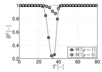
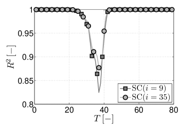
(a)	(b)

Figure 4: Evolution of $R^{2}$: (a) as a function of degree of PCE ($i=35$); (b) as a function of sparse grid points ($p=5$)

Figs. 4(a)-(b) display the evolution of the coefficient of determination $R^{2}$ in all time steps of numerical example. It is evident that the surrogate model is less accurate when the elastic limit is reached and the model response is not smooth. This phenomenon is displayed in Figs. 5(a)-(b) where two examples of PC expansions corresponding to time steps $T=29$ and $T=34$, respectively, are plotted as functions of random variable $\xi_{1}$ and compared with the reference MC solution. One can see that as a consequence of active yielding, the model response $\sigma_{11}\,\mathrm{[Pa]}$ is not smooth, but close to bilinear, which is difficult to be approximated by low order polynomials. On the other hand, Fig 4(b) points out that once having sufficient polynomial degree, increasing the number collocation points does not lead to significant improvement of surrogate quality as documented also by results in Tab. 2.

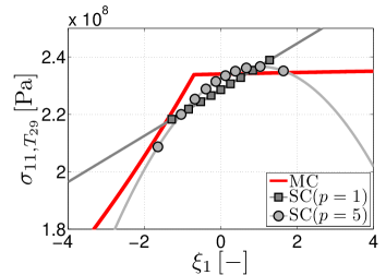
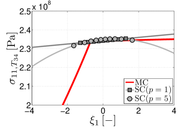
(a)	(b)

Figure 5: Shape of critical PC expansions corresponding to (a) $T=29$ and (b) $T=34$.

Several interesting results have been derived within the scope of numerical calculations with all uncertain parameters as an input. We consider all the parameters to be lognormally distributed with prescribed mean $\mu_{q}$ and standard deviation $\sigma^{\mathrm{STD}}_{q}$ given in Tab. 3.

Symbol	Type of variable	Value	Mean ($\mu_{q}$)	Standard deviation ($\sigma^{\mathrm{STD}}_{q}$)
$E$	lognormal RV	-	$210\cdot 10^{9}$	$21\cdot 10^{9}$
$\nu$	lognormal RV	-	$0.3$	$0.015$
$\sigma_{\mathrm{y,0}}$	lognormal RV	-	$235\cdot 10^{6}$	$23.5\cdot 10^{6}$
$H$	lognormal RV	-	$21\cdot 10^{8}$	$2.1\cdot 10^{8}$

Table 3: Input parameters of numerical study

In addition, the uniaxial tensile problem is extended by load/unload cycle resulting in $300$ uniform time steps $T$ of numerical analysis. Fig. 6 presents the reference MC solution obtained for $10^{6}$ samples.

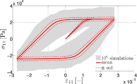
Figure 6: Reference MC simulations corresponding to material parameters in Tab. 3, evolution of model response $\sigma_{11}\,\mathrm{[Pa]}$ as function of $\varepsilon_{11}\,\mathrm{[-]}$

	$p$ $/$ $i$	201	3065	12057	20681
$e(\mu_{\sigma_{11}})$	-	$3.6\cdot 10^{-3}$	$1.1\cdot 10^{-3}$	$3.1\cdot 10^{-4}$	$2.3\cdot 10^{-4}$
$e(\sigma^{\mathrm{STD}}_{\sigma_{11}})$	1	$7.9\cdot 10^{-2}$	$7.8\cdot 10^{-2}$	$7.8\cdot 10^{-2}$	$7.8\cdot 10^{-2}$
	5	$2.3\cdot 10^{-2}$	$6.4\cdot 10^{-3}$	$3.7\cdot 10^{-3}$	$3.8\cdot 10^{-3}$
	15	–	–	$2.2\cdot 10^{-3}$	$1.6\cdot 10^{-3}$
$e(Q^{0.01}_{\sigma_{11}})$	1	$4.1\cdot 10^{-2}$	$4.1\cdot 10^{-2}$	$4.1\cdot 10^{-2}$	$4.1\cdot 10^{-2}$
	5	$1.3\cdot 10^{-2}$	$7.6\cdot 10^{-3}$	$7.2\cdot 10^{-3}$	$7.1\cdot 10^{-3}$
	15	–	–	$2.5\cdot 10^{-3}$	$2.4\cdot 10^{-3}$

Table 4: Errors of surrogate models calculated for different degree of PC expansion $p$ and number of collocation points $i$

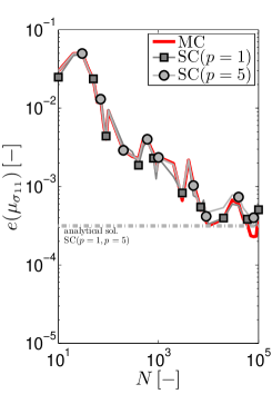
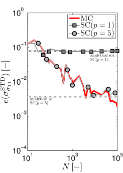
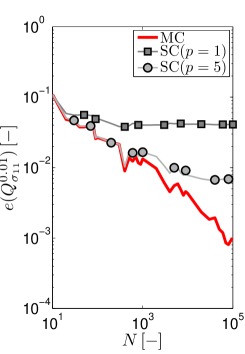
(a)	(b)	(c)
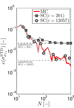
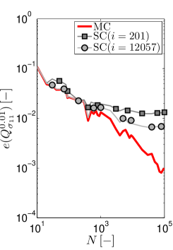
(d)	(e)	(f)

Figure 7: Error analysis of (a) mean $\mu\,\mathrm{[-]}$, (b) standard deviation $\sigma^{\mathrm{STD}}\,\mathrm{[-]}$ and (c) quantile $Q^{0.01}\,\mathrm{[-]}$ for fixed number of sparse grid points $(i=12057)$; (d) Error analysis of mean $\mu\,\mathrm{[-]}$, (e) standard deviation $\sigma^{\mathrm{STD}}\,\mathrm{[-]}$ and (f) quantile $Q^{0.01}\,\mathrm{[-]}$ for fixed degree of PCE $(p=5)$

The Eqs. (20) – (21) are utilised again to asses the accuracy of surrogate model. Figs. 7(a)-(b) and Tab. 4 display the results of error analysis for predicting mean $\mu$, standard deviation $\sigma^{\mathrm{STD}}$ and quantile $Q^{0.01}$ of a model response $\sigma_{11}$. The errors exhibit very similar convergence with increasing number of collocation points and degree of polynomials as in previous example.

The coefficient of determination $R^{2}$ is plotted in Figs. 8(a)-(b) to quantify the overall accuracy of surrogate models in particular time steps. The lower quality of PC expansion is caused again by nonlinearity in the stochastic solution near elastic limit of material.

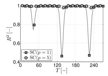
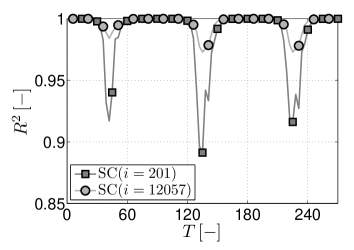
(a)	(b)

Figure 8: Evolution of $R^{2}$: (a) Function of degree of PCE ($i=12057$); (b) Function of sparse grid points ($p=5$)

The evolution of time requirements as a function of number of samples $N$ is presented in Fig. 9 for MC computations and PC-based computations performed for different number of collocation points ($i=201$, $i=12057$). PC-based predictions of mean $\mu$ and standard deviations $\sigma^{\mathrm{STD}}$ are obtained analytically, while predictions of quantile $Q^{0.01}$ are computed by MC sampling with $N=10^{5}$ samples.

Computational time required for prediction of mean is composed mainly by the time necessary for evaluation of collocation points, because only the constant term of PCE needs to be calculated and the corresponding computational time is negligible. Fig. 9(a) shows that time requirements of MC-based and PC-based predictions are comparable, which indicates that the organisation of collocation points does not bring any significant advantage comparing to randomicity of MC method. This may be caused by high nonlinearity of the model, which needs to be described by higher order polynomials constructed on higher number of collocation points as suggested by better result of PC-based predictions for $i=20681$ points.

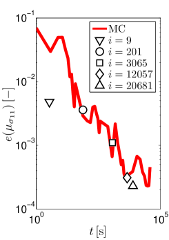
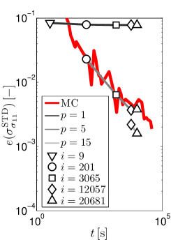
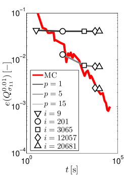
(a)	(b)	(c)

Figure 9: Error analysis of (a) mean $\mu\,\mathrm{[-]}$, (b) standard deviation $\sigma^{\mathrm{STD}}\,\mathrm{[-]}$ and (c) quantile $Q^{0.01}\,\mathrm{[-]}$ as a function of computational time

Similar phenomenon may be observed also in Fig. 9(b), where PC-based predictions outperform results of MC method also for higher number of collocation points. Nevertheless, a significant role is also played by the polynomial order used and thus the computational time includes here also the time needed for calculation of all the polynomial terms. This time is however still negligible compared to the time needed for the evaluation of collocation points as visible in Fig. 9(b). Here, the points corresponding to the same number of collocation points but different polynomial order have almost identical time coordinate. This observation suggests an important conclusion and recommendation to use the highest polynomial order possible for a given number of collocation points – in Figs. 9(b)-(c), this situation correspond to left ends of lines corresponding to particular polynomial orders.

The same conclusion may be done regarding Fig. 9(c), even though here the computational time needed for PC-based predictions includes also inevitable time for MC-sampling of the polynomials with $N=10^{5}$ samples, which seems again negligible, relatively compared to the time for evaluation of collocation points. The number of MC samples of polynomials is chosen with respect to Figs. 7(c) and 7(f), where the curves of prediction errors seems to be stabilised between $N=10^{4}$ and $N=10^{5}$ samples and higher number of samples will probably not change the results. It is also interesting to point out the negligible effect of increasing number of collocation points for an unchanged polynomial order leading to waste of computational time and worse results than MC-based predictions.

6 Conclusions

This paper presents the numerical modelling of elasto-plastic material behavior described by the uncertain parameters. In particular, we employed the Maxwell–Huber–Hencky–von Mises model, which is sufficiently robust to describe real-world materials such as metals, but which is also nonlinear and time-dependent material model. In order to investigate the presence of uncertainty on material response, we replace the expensive MC simulations of computational model by its cheaper approximation based on PCE computed by SC method. The whole concept is demonstrated on two simple examples of uniaxial test at a material point, where interesting phenomena can be clearly understood. First example consider only loading path and Young’s modulus to be uncertain, while the second example is extended by load/unload cycle and uncertainty assumed in all the four material parameters: Young’s modulus, Poisson’s ratio, initial yield strength and hardening parameter. The quality of obtained surrogate models is compared to MC method in terms of accuracy as well as the time requirements. Figs. 9(a)-(c) show that the second example represent situation where time requirements are mainly driven by time needed for evaluation of collocation points and PC construction is negligible. However, the PC-based predictions achieve also similar accuracy as MC-based predictions for equal number of sampling and collocation points as demonstrated in Figs. 7(a)-(f). Therefore, the PC-based approximation does not bring an important acceleration in this example. In the first example, the computational time of model simulation is too small for any reliable measurement. Nevertheless, we may point out the results in Figs. 3(a)-(f), where only $35$ collocation points need to be computed for prediction of mean and standard deviation with errors comparable to MC-based predictions obtained for more than $10^{3}$ samples. Hence, the significant acceleration by PC-based approximation cannot be guaranteed generally, but definitely remains interesting and worthy to apply.

References

- [1] Anders, M., Hori, M.: Stochastic finite element method for elasto-plastic body, International Journal for Numerical Methods in Engineering, 46, 11, 1999, pp. 1897–1916.
- [2] Arnst, M., Ghanem, R.: A variational-inequality approach to stochastic boundary value problems with inequality constraints and its application to contact and elastoplasticity, International Journal for Numerical Methods in Engineering, 89, 2012, pp. 1665–1690.
- [3] Babuška, I., Tempone, R., Zouraris, G. E.: Galerkin Finite Element Approximations of Stochastic Elliptic Partial Differential Equations, SIAM Journal on Numerical Analysis, 42, 2, 2004, pp. 800–825.
- [4] Babuška, I., Nobile, F., Tempone, R.: A Stochastic Collocation Method for Elliptic Partial Differential Equations with Random Input Data. SIAM Journal on Numerical Analysis, 45, 3, 2007, pp. 1005–1034.
- [5] Blatman, G., Sudret, B.: An adaptive algorithm to build up sparse polynomial chaos expansions for stochastic finite element analysis, Probabilistic Engineering Mechanics, 25, 2, 2010, pp. 183–197.
- [6] Dunne, F., Petrinic, N.: Introduction to Computational Plasticity, Oxford University Press, 2005.
- [7] Evans, M., Swartz, T.: Methods for approximating integrals in statistics with special emphasis on Bayesian integration problems, Statistical Science, 10, 3, 1995, pp. 254–272.
- [8] Ghanem, R. G., Spanos, P. D.: Stochastic Finite Elements: A Spectral Approach, Dover Publications, Revised edition, 2012.
- [9] Grassl, P., Jirásek, J.: Damage-plastic model for concrete failure, International Journal of Solids and Structures, 43, 2006, pp. 7166–7196.
- [10] Gutiérrez, M., Krenk, S.: Encyclopedia of Computational Mechanics, chap. Stochastic finite element methods, John Wiley & Sons, Ltd., 2004.
- [11] Heiss, F., Winschel, V.: Likelihood approximation by numerical integration on sparse grids, Journal of Econometrics, 144, 1, 2008, pp. 62–80.
- [12] Horák, M.: Localization Analysis of Damage and Plasticity Models, Master thesis, CTU in Prague, 2009.
- [13] Keese, A.: A review of recent developments in the numerical solution of stochastic partial differential equations (stochastic finite elements), Tech. rep., Institute of Scientific Computing, Technical University Braunschweig, 2003.
- [14] Krieg, R. D., Krieg, D. B.: Accuracies of Numerical Solution Methods for the Elastic-Perfectly Plastic Model, Journal of Pressure Vessel Technology, 99, 4, 1977, pp. 510–515.
- [15] Keese, A., Matthies, H. G.: Hierarchical parallelisation for the solution of stochastic finite element equations, Computers and Structures, 83, 2005, pp. 1033–1047.
- [16] Kučerová, A., Sýkora, J., Rosić, B., Matthies, H. G.: Acceleration of uncertainty updating in the description of transport processes in heterogeneous materials, Journal of Computational and Applied Mathematics, 236, 18, 2012, pp. 4862–4872.
- [17] Kučerová, A., Sýkora, J.: Uncertainty updating in the description of coupled heat and moisture transport in heterogeneous materials, Applied Mathematics and Computation, 219, 2013, pp. 7252–7261.
- [18] Lourenço, P. B., de Borst, R., Rots, J. G.: A plane stress softening plasticity model for orthotropic materials, International Journal for Numerical Methods in Engineering, 40, 1997, pp. 4033–4057.
- [19] Marzouk, Y., Najm, H., Rahn, L.: Stochastic Spectral Methods for Efficient Bayesian Solution of Inverse Problems, Journal of Computational Physics, 224, 2, 2007, pp. 560–586.
- [20] Matthies, H. G.: Encyclopedia of Computational Mechanics, chap. Uncertainty Quantification with Stochastic Finite Elements. John Wiley & Sons, Ltd., 2007.
- [21] Rosić, B., Matthies, H. G.: Computational Approaches to Inelastic Media with Uncertain Parameters, Journal of the Serbian Society for Computational Mechanics, 2, 1, 2008, pp. 28–43.
- [22] Rosić, B.: Variational Formulations and Functional Approximation Algorithms in Stochastic Plasticity of Materials, PhD thesis, Institute of Scientific Computing, Technical University Braunschweig, 2012.
- [23] Steel, R. G. D, Torrie, J. H.: Principles and Procedures of Statistics with Special Reference to the Biological Sciences, McGraw Hill, 1960.
- [24] Stefanou, G.: The stochastic finite element method: Past, present and future, Computer Methods in Applied Mechanics and Engineering, 198, 9-12, 2009, pp. 1031–1051.
- [25] Wiener, N.: The Homogeneous Chaos, American Journal of Mathematics, 60, 4, 1938, pp. 897–936.
- [26] Xiu, D., Karniadakis, G. E.: The Wiener Askey Polynomial Chaos for Stochastic Differential Equations, SIAM Journal on Scientific Computing, 24, 2, 2002, pp. 619–644.
- [27] Xiu, D., Hesthaven, J. S.: High-Order Collocation Methods for Differential Equations with Random Inputs, SIAM Journal on Scientific Computing, 27, 3, 2005, pp. 1118–1139.
- [28] Xiu, D.: Fast Numerical Methods for Stochastic Computations: A Review, Communications in Computational Physics, 5, 2-4, 2009, pp. 242–272.