Dual Query: Practical Private Query Release
for High Dimensional Data

Abstract

We present a practical, differentially private algorithm for answering a large number of queries on high dimensional datasets. Like all algorithms for this task, ours necessarily has worst-case complexity exponential in the dimension of the data. However, our algorithm packages the computationally hard step into a concisely defined integer program, which can be solved non-privately using standard solvers. We prove accuracy and privacy theorems for our algorithm, and then demonstrate experimentally that our algorithm performs well in practice. For example, our algorithm can efficiently and accurately answer millions of queries on the Netflix dataset, which has over $17{,}000$ attributes; this is an improvement on the state of the art by multiple orders of magnitude.

1 Introduction

Privacy is becoming a paramount concern for machine learning and data analysis tasks, which often operate on personal data. For just one example of the tension between machine learning and data privacy, Netflix released an anonymized dataset of user movie ratings for teams competing to develop an improved recommendation mechanism. The competition was a great success (the winning team improved on the existing recommendation system by more than $10\%$), but the ad hoc anonymization was not as successful: Narayanan and Shmatikov [28] were later able to re-identify individuals in the dataset, leading to a lawsuit and the cancellation of subsequent competitions.

Differentially private query release is an attempt to solve this problem. Differential privacy is a strong formal privacy guarantee (that, among other things, provably prevents re-identification attacks), and the problem of query release is to release accurate answers to a set of statistical queries. As observed early on by Blum et al. [5], performing private query release is sufficient to simulate any learning algorithm in the statistical query model of Kearns [23].

Since then, the query release problem has been extensively studied in the differential privacy literature. While simple perturbation can privately answer a small number of queries [14], more sophisticated approaches can accurately answer nearly exponentially many queries in the size of the private database [4, 12, 13, 31, 19, 17, 20]. A natural approach, employed by many of these algorithms, is to answer queries by generating synthetic data: a safe version of the dataset that approximates the real dataset on every statistical query of interest.

Unfortunately, even the most efficient approaches for query release have a per-query running time linear in the size of the data universe—the number of possible kinds of records. If each record is specified by a set of attributes, the size of the data universe is exponential in the number of attributes [19]. Moreover, this running time is necessary in the worst case [35, 36].

This exponential runtime has hampered practical evaluation of query release algorithms. One notable exception is due to Hardt et al. [20], who perform a thorough experimental evaluation of one such algorithm, which they called MWEM (Multiplicative Weights Exponential Mechanism). They find that MWEM has quite good accuracy in practice and scales to higher dimensional data than suggested by a theoretical (worst-case) analysis. Nevertheless, running time remains a problem, and the approach does not seem to scale to high dimensional data (with more than $30$ or so attributes for general queries, and more when the queries have more structure). The critical bottleneck is the size of the state maintained by the algorithm: MWEM, like many query release algorithms, needs to manipulate an object that has size linear in the size of the data universe. This quickly becomes impractical for records with even a modest number of attributes.

We present DualQuery, an alternative algorithm which is dual to MWEM in a sense that we will make precise. Rather than manipulating an object of exponential size, DualQuery solves a concisely represented (but NP-hard) optimization problem. Critically, the optimization step does not require a solution that is private or exact, so it can be handled by existing, highly optimized solvers. Except for this step, all parts of our algorithm are efficient. As a result, DualQuery requires (worst-case) space and (in practice) time only linear in the number of queries of interest, which is often significantly smaller than the size of the data universe. Like existing algorithms for query release, DualQuery has a provable accuracy guarantee and satisfies the strong differential privacy guarantee. Both DualQuery and MWEM generate synthetic data: the output of both algorithms is a data set from the same domain as the input data set, and can thus be used as the original data set would have been used. It is important to note that the that the output data set is guaranteed to be similar to the input data set only with respect to the query class; the synthetic data might not be similar to the real data in other respects.

We evaluate DualQuery on a variety of datasets by releasing 3-way marginals (also known as conjunctions or contingency tables), demonstrating that it solves the query release problem accurately and efficiently even when the data includes hundreds of thousands of features. We know of no other algorithm that can perform accurate, private query release for this class of queries on real data with more than even $100$ features.

Related work

Differentially private learning has been studied since Blum et al. [5] showed how to convert learning algorithms in the SQ model of Kearns [23] into differentially private learning algorithms with similar accuracy guarantees. Since then, private machine learning has become a very active field with both foundational sample complexity results [22, 6, 3, 11] and numerous efficient algorithms for particular learning problems [7, 9, 32, 24, 10, 33].

In parallel, there has been a significant amount of work on privately releasing synthetic data based on a true dataset while preserving the answers to large numbers of statistical queries [4, 12, 31, 13, 19, 17]. These results are extremely strong in an information theoretic sense: they ensure the consistency of the synthetic data with respect to an exponentially large family of statistics. But, all of these algorithms (including the notable multiplicative weights algorithm of Hardt and Rothblum [19], which achieves the theoretically optimal accuracy and runtime) have running time exponential in the dimension of the data. Under standard cryptographic assumptions, this is necessary in the worst case for mechanisms that answer arbitrary statistical queries [35].

Nevertheless, there have been some experimental evaluations of these approaches on real datasets. Most related to our work is the evaluation of the MWEM mechanism by Hardt et al. [20], which is based on the private multiplicative weights mechanism [19]. This algorithm is inefficient—it manipulates a probability distribution over a set exponentially large in the dimension of the data space—but with some heuristic optimizations, Hardt et al. [20] were able to implement the multiplicative weights algorithm on real datasets with up to 77 attributes (and even more when the queries are restricted to take positive values only on a small number of disjoint groups of features). However, it seems difficult to scale this approach to higher dimensional data.

Another family of query release algorithms are based on the Matrix Mechanism [26, 25]. The runtime guarantees of the matrix mechanism are similar to the approaches based on multiplicative weights—the algorithm manipulates a “matrix” of queries with dimension exponential in the number of features. Yaroslavtsev et al. [37] evaluate an approach based on this family of algorithms on low dimensional datasets, but scaling to high dimensional data also seems challenging. A recent work by Zhang et al. [38] proposes a low-dimensional approximation for high-dimensional data distribution by privately constructing Bayesian networks, and shows that such a representation gives good accuracy on some real datasets.

Our algorithm is inspired by the view of the synthetic data generation problem as a zero-sum game, first proposed by Hsu et al. [21]. In this interpretation, Hardt et al. [20] solves the game by having a data player use a no-regret learning algorithm, while the query player repeatedly best responds by optimizing over queries. In contrast, our algorithm swaps the roles of the two players: the query player now uses the no-regret learning algorithm, whereas the data player now finds best responses by solving an optimization problem. This is reminiscent of “Boosting for queries,” proposed by Dwork et al. [13]; the main difference is that our optimization problem is over single records rather than sets of records. As a result, our optimization can be handled non-privately.

There is also another theoretical approach to query release due to Nikolov, Talwar, and Zhang (and later specialized to marginals by Dwork, Nikolov, and Talwar) that shares a crucial property of the one we present here—namely that the computationally difficult step does not need to be solved privately [30, 15]. The benefit of our approach is that it yields synthetic data rather than just query answers, and that the number of calls to the optimization oracle is smaller. However, the approach of Nikolov et al. [30], Dwork et al. [15] yields theoretically optimal accuracy bounds (ours does not), and so that approach certainly merits future empirical evaluation.

2 Differential privacy background

Differential privacy has become a standard algorithmic notion for protecting the privacy of individual records in a statistical database. It formalizes the requirement that the addition or removal of a data record does not change the probability of any outcome of the mechanism by much.

To begin, databases are multisets of elements from an abstract domain $\mathcal{X}$, representing the set of all possible data records. Two databases $D,D^{\prime}\subset\mathcal{X}$ are neighboring if they differ in a single data element ($|D\triangle D^{\prime}|\leq 1$).

Definition 2.1 (Dwork et al. [14]).

A mechanism $M\colon\mathcal{X}^{n}\rightarrow R$ satisfies $(\varepsilon,\delta)$-differential privacy if for every $S\subseteq R$ and for all neighboring databases $D,D^{\prime}\in\mathcal{X}^{n}$, the following holds:

$$\Pr[M(D)\in S]\leq e^{\varepsilon}\Pr[M(D^{\prime})\in S]+\delta$$

If $\delta=0$ we say $M$ satisfies $\varepsilon$-differential privacy.

Definition 2.2.

The (global) sensitivity of a query $q$ is its maximum difference when evaluated on two neighboring databases:

$$GS_{f}=\max_{D,D^{\prime}\in\mathcal{X}^{n}:|D\triangle D^{\prime}|=1}|q(D)-q(D^{\prime})|.$$

In this paper, we consider the private release of information for the classes of linear queries, which have sensitivity $1/n$.

Definition 2.3.

For a predicate $\varphi\colon\mathcal{X}\rightarrow\{0,1\}$, the linear query $q_{\varphi}\colon\mathcal{X}^{n}\rightarrow[0,1]$ is defined by

$$q_{\varphi}(D)=\frac{\sum_{x\in D}\varphi(x)}{|D|}.$$

We will often represent linear queries a different form, as a vector $q\in\{0,1\}^{|\mathcal{X}|}$ explicitly encoding the predicate $\phi$:

$$q(D)=\frac{\sum_{x\in D}q_{x}}{|D|}.$$

We will use a fundamental tool for private data analysis: we can bound the privacy cost of an algorithm as a function of the privacy costs of its subcomponents.

Lemma 2.4 (Dwork et al. [13]).

Let $M_{1},\ldots,M_{k}$ be such that each $M_{i}$ is $(\varepsilon_{i},0)$-private with $\varepsilon_{i}\leq\varepsilon^{\prime}$. Then $M(D)=(M_{1}(D),\ldots,M_{k}(D))$ is $(\varepsilon,0)$-private for $\varepsilon=\sum_{i=1}^{k}\varepsilon_{i},$ and $(\varepsilon,\delta)$-private for

$$\varepsilon=\sqrt{2\log(1/\delta)k}\varepsilon^{\prime}+k\varepsilon^{\prime}(e^{\varepsilon^{\prime}}-1)$$

for any $\delta\in(0,1)$. The sequence of mechanisms can be chosen adaptively, i.e., later mechanisms can take outputs from previous mechanisms as input.

3 The query release game

The analysis of our algorithm relies on the interpretation of query release as a two player, zero-sum game [21]. In the present section, we review this idea and related tools.

Game definition

Suppose we want to answer a set of queries $\mathcal{Q}$. For each query $q\in\mathcal{Q}$, we can form the negated query $\overline{q}$, which takes values $\overline{q}(D)=1-q(D)$ for every database $D$. Equivalently, for a linear query defined by a predicate $\varphi$, the negated query is defined by the negation $\neg\varphi$ of the predicate. For the remainder, we will assume that $\mathcal{Q}$ is closed under negation; if not, we may add negated copies of each query to $\mathcal{Q}$.

Let there be two players, whom we call the data player and query player. The data player has action set equal to the data universe $\mathcal{X}$, while the query player has action set equal to the query class $\mathcal{Q}$. Given a play $x\in\mathcal{X}$ and $q\in\mathcal{Q}$, we let the payoff be

$$A(x,q):=q(D)-q(x),$$ (1)

where $D$ is the true database. To define the zero-sum game, the data player will try to minimize the payoff, while the query player will try to maximize the payoff.

Equilibrium of the game

Let $\Delta(\mathcal{X})$ and $\Delta(\mathcal{Q})$ be the set of probability distributions over $\mathcal{X}$ and $\mathcal{Q}$. We consider how well each player can do if they randomize over their actions, i.e., if they play from a probability distribution over their actions. By von Neumann’s minimax theorem,

$$\min_{u\in\Delta(\mathcal{X})}\max_{w\in\Delta(\mathcal{Q})}A(u,w)=\max_{w\in\Delta(\mathcal{Q})}\min_{u\in\Delta(\mathcal{X})}A(u,w),$$

for any two player zero-sum game, where

$$A(u,w):=\mathbb{E}_{x\sim u,q\sim w}A(x,q)$$

is the expected payoff. The common value is called the value of the game, which we denote by $v_{A}$.

Intuitively, von Neumann’s theorem states that there is no advantage in a player going first: the minimizing player can always force payoff at most $v_{A}$, while the maximizing player can always force payoff at least $v_{A}$. This suggests that each player can play an optimal strategy, assuming best play from the opponent—this is the notion of equilibrium strategies, which we now define. We will soon interpret these strategies as solutions to the query release problem.

Definition 3.1.

Let $\alpha>0$. Let $A$ be the payoffs for a two player, zero-sum game with action sets $\mathcal{X},\mathcal{Q}$. Then, a pair of strategies $u^{*}\in\Delta(\mathcal{X})$ and $w^{*}\in\Delta(\mathcal{Q})$ form an $\alpha$-approximate mixed Nash equilibrium if

$$A(u^{*},w)\leq v_{A}+\alpha\qquad\text{and}\qquad A(u,w^{*})\geq v_{A}-\alpha$$

for all strategies $u\in\Delta(\mathcal{X})$ and $w\in\Delta(\mathcal{Q})$.

If the true database $D$ is normalized to be a distribution $\widehat{D}$ in $\Delta(\mathcal{X})$, then $\widehat{D}$ always has zero payoff:

$$A(\widehat{D},w)=\mathbb{E}_{x\sim\widehat{D},q\sim w}[q(D)-q(x)]=0.$$

Hence, the value of the game $v_{A}$ is at most $0$. Also, for any data strategy $u$, the payoff of query $q$ is the negated payoff of the negated query $\overline{q}$:

$$A(u,\overline{q}) =\mathbb{E}_{x\sim u}[\overline{q}(D)-\overline{q}(x)]=\mathbb{E}_{x\sim u}[q(x)-q(D)],$$

which is $A(u,\overline{q})$. Thus, any query strategy that places equal weight on $q$ and $\overline{q}$ has expected payoff zero, so $v_{A}$ is at least $0$. Hence, $v_{A}=0$.

Now, let $(u^{*},w^{*})$ be an $\alpha$-approximate equilibrium. Suppose that the data player plays $u^{*}$, while the query player always plays query $q$. By the equilibrium guarantee, we then have $A(u^{*},q)\leq\alpha$, but the expected payoff on the left is simply $q(D)-q(u^{*})$. Likewise, if the query player plays the negated query $\overline{q}$, then

$$-q(D)+q(u^{*})=A(u^{*},\overline{q})\leq\alpha,$$

so $q(D)-q(u^{*})\geq-\alpha$. Hence for every query $q\in\mathcal{Q}$, we know $|q(u^{*})-q(D)|\leq\alpha$. This is precisely what we need for query release: we just need to privately calculate an approximate equilibrium.

Solving the game

To construct the approximate equilibrium, we will use the multiplicative weights update algorithm (MW). This algorithm maintains a distribution over actions (initially uniform) over a series of steps. At each step, the MW algorithm receives a (possibly adversarial) loss for each action. Then, MW reweights the distribution to favor actions with less loss. The algorithm is presented in Algorithm 1.

  Let $\eta>0$ be given, let $\mathcal{A}$ be the action space

  Initialize $\widetilde{A}^{1}$ uniform distribution on $\mathcal{A}$

  For $t=1,2,\dots,T$:

     Receive loss vector $\ell^{t}$

     For each $a\in\mathcal{A}$:

        Update $A^{t+1}_{a}=e^{-\eta\ell^{t}_{a}}\widetilde{A}^{t}_{a}$ for every $a\in\mathcal{A}$

     Normalize $\widetilde{A}^{t+1}=\frac{A^{t+1}}{\sum_{i}A^{t+1}_{i}}$

Algorithm 1 The Multiplicative Weights Algorithm

For our purposes, the most important application of MW is to solving zero-sum games. Freund and Schapire [16] showed that if one player maintains a distribution over actions using MW, while the other player selects a best-response action versus the current MW distribution (i.e., an action that maximizes his expected payoff), the average MW distribution and empirical best-response distributions will converge to an approximate equilibrium rapidly.

Theorem 3.2 (Freund and Schapire [16]).

Let $\alpha>0$, and let $A(i,j)\in[-1,1]^{m\times n}$ be the payoff matrix for a zero-sum game. Suppose the first player uses multiplicative weights over their actions to play distributions $p^{1},\dots,p^{T}$, while the second player plays $(\alpha/2)$-approximate best responses $x^{1},\dots,x^{T}$, i.e.,

$$A(x^{t},p^{t})\geq\max_{x}A(x,p^{t})-\alpha/2.$$

Setting $T=16\log n/\alpha^{2}$ and $\eta=\alpha/4$ in the MW algorithm, the empirical distributions

$$\frac{1}{T}\sum_{i=1}^{T}p^{i}\quad\text{and}\quad\frac{1}{T}\sum_{i=1}^{T}x^{i}$$

form an $\alpha$-approximate mixed Nash equilibrium.

4 Dual query release

Viewing query release as a zero-sum game, we can interpret the algorithm of Hardt and Rothblum [19] (and the MWEM algorithm of Hardt et al. [20]) as solving the game by using MW for the data player, while the query player plays best responses. To guarantee privacy, their algorithm selects the query best-responses privately via the exponential mechanism of McSherry and Talwar [27]. Our algorithm simply reverses the roles: while MWEM uses a no-regret algorithm to maintain the data player’s distribution, we will instead use a no-regret algorithm for the query player’s distribution; instead of finding a maximum payoff query at each round, our algorithm selects a minimum payoff record at each turn.

In a bit more detail, we maintain a distribution $\mathcal{Q}$ over the queries, initially uniform. At each step $t$, we first simulate the data player making a best response against $\mathcal{Q}$, i.e., selecting a record $x^{t}$ that maximizes the expected payoff if the query player draws a query according to $\mathcal{Q}$. As we discuss below, for privacy considerations we cannot work directly with the distribution $\mathcal{Q}$. Instead, we sample $s$ queries $\{q_{i}\}$ from $\mathcal{Q}$, and form “average” query $\widetilde{q}$, which we take as an estimate of the true distribution $\mathcal{Q}$. The data player then best-responds against $\widetilde{q}$.

Then, we simulate the query player updating the distribution $\mathcal{Q}$ after seeing the selected record $x^{t}$—we will reduce weight on queries that have similar answers on $x^{t}$ the database $D$, and we will increase weight on queries that have very different answers on $x^{t}$ and $D$. After running for $T$ rounds, we output the set of records $\{x_{t}\}_{t}$ as the synthetic database. Note that this is a data set from the same domain as the original data set, and so can be used in any application that the original data set can be used in – with the caveat of course, that except with respect to the query class used in the algorithm, there are no guarantees about how the synthetic data resembles the real data. The full algorithm can be found in Algorithm 2; the main parameters are $\alpha\in(0,1)$, which is the target maximum additive error of any query on the final output, and $\beta\in(0,1)$, which is the probability that the algorithm may fail to achieve the accuracy level $\alpha$. These parameters two control the number of steps we take ($T$), the update rate of the query distribution ($\eta$), and the number of queries we sample at each step ($s$).

Our privacy argument differs slightly from the analysis for MWEM. There, the data distribution is public, and finding a query with high error requires access to the private data. Our algorithm instead maintains a distribution $Q$ over queries which depends directly on the private data, so we cannot use $Q$ directly. Instead, we argue that queries sampled from $Q$ are privacy preserving. Then, we can use a non-private optimization method to find a minimal error record versus queries sampled from $Q$. We then trade off privacy (which degrades as we take more samples) with accuracy (which improves as we take more samples, since the distribution of sampled queries converges to $Q$).

Given known hardness results for the query release problem [35], our algorithm must have worst-case runtime polynomial in the universe size $|\mathcal{X}|$, so is not theoretically more efficient than prior approaches. In fact, even compared to prior work on query release (e.g., Hardt and Rothblum [19]), our algorithm has a weaker accuracy guarantee. However, our approach has an important practical benefit: the computationally hard step can be handled with standard, non-private solvers (we note that this is common also to the approach of [30, 15]).

The iterative structure of our algorithm, combined with our use of constraint solvers, also allows for several heuristics improvements. For instance, we may run for fewer iterations than predicted by theory. Or, if the optimization problem turns out to be hard (even in practice), we can stop the solver early at a suboptimal (but often still good) solution. These heuristic tweaks can improve accuracy beyond what is guaranteed by our accuracy theorem, while always maintaining a strong provable privacy guarantee.

  Parameters: Target accuracy level $\alpha\in(0,1)$, target failure probability $\beta\in(0,1)$.

  Input: Database $D\in\mathbb{R}^{|\mathcal{X}|}$ (normalized) and linear queries $q_{1},\dots,q_{k}\in\{0,1\}^{|\mathcal{X}|}$.

  Initialize: Let $\mathcal{Q}=\bigcup_{j=1}^{k}q_{j}\cup\overline{q_{j}}$, $Q^{1}$ be a uniform distribution on $\mathcal{Q}$,

$$T=\frac{16\log|\mathcal{Q}|}{\alpha^{2}},\qquad\eta=\frac{\alpha}{4},\qquad\text{and}\qquad s=\frac{48\log\left({2|\mathcal{X}|T}/{\beta}\right)}{\alpha^{2}}.$$

Let the payoff function $A_{D}:\mathcal{X}\times[0,1]^{|\mathcal{X}|}\to\mathbb{R}$ be:

$$A_{D}(x,\widetilde{q})=\widetilde{q}(D)-\widetilde{q}(x),\qquad\text{where}\qquad\widetilde{q}(D)=\frac{1}{|D|}\sum_{x\in D}\widetilde{q}_{x}.$$

  For $t=1,\dots,T$:

     Sample $s$ queries $\{q_{i}\}$ from $\mathcal{Q}$ according to $Q^{t}$.

     Let $\widetilde{q}:=\frac{1}{s}\sum_{i}q_{i}$.

     Find $x^{t}$ with $A_{D}(x^{t},\widetilde{q})\geq\max_{x}A_{D}(x,\widetilde{q})-\alpha/4$.

     Update: For each $q\in\mathcal{Q}$:

        $Q^{t+1}_{q}:=\exp(-\eta A_{D}(x^{t},q)\rangle)\cdot Q^{t}_{q}.$

     Normalize $Q^{t+1}$.

  Output synthetic database $\widehat{D}:=\bigcup_{t=1}^{T}x^{t}.$

Algorithm 2 DualQuery

Privacy

The privacy proofs are largely routine, based on the composition theorems. Rather than fixing $\varepsilon$ and solving for the other parameters as is typical in the literature, we present the privacy cost $\varepsilon$ as function of parameters $T,s,\eta$. This form will lead to simpler tuning of the parameters in our experimental evaluation.

We will use the privacy of the following mechanism (result due to McSherry and Talwar [27]) as an ingredient in our privacy proof.

Lemma 4.1 (McSherry and Talwar [27]).

Given some arbitrary output range $R$, the exponential mechanism with score function $S$ selects and outputs an element $r\in R$ with probability proportional to

$$\exp\left(\frac{\varepsilon S(D,r)}{2\cdot GS_{S}}\right),$$

where $GS_{S}$ is the sensitivity of $S$, defined as

$$GS_{S}=\max_{D,D^{\prime}:|D\triangle D^{\prime}|=1,r\in R}|S(D,r)-S(D^{\prime},r)|.$$

The exponential mechanism is $\varepsilon$-differentially private.

We first prove pure $\varepsilon$-differential privacy.

Theorem 4.2.

DualQuery is $\varepsilon$-differentially private for

$$\varepsilon=\frac{\eta T(T-1)s}{n}.$$

Proof.

We will argue that sampling from $Q^{t}$ is equivalent to running the exponential mechanism with some quality score. At round $t$, let $\{x^{i}\}$ for $i\in[t-1]$ be the best responses for the previous rounds. Let $r(D,q)$ be defined by

$$r(D,q)=\sum_{i=1}^{t-1}(q(D)-q(x^{i})),$$

where $q\in\mathcal{Q}$ is a query and $D$ is the true database. This function is evidently $((t-1)/n)$-sensitive in $D$: changing $D$ changes each $q(D)$ by at most $1/n$. Now, note that sampling from $Q^{t}$ is simply sampling from the exponential mechanism, with quality score $r(D,q)$. Thus, the privacy cost of each sample in round $t$ is $\varepsilon_{t}^{\prime}=2\eta(t-1)/n$ by Lemma 4.1.

By the standard composition theorem (Lemma 2.4), the total privacy cost is

$$\varepsilon=\sum_{t=1}^{T}s\varepsilon_{t}^{\prime}=\frac{2\eta s}{n}\cdot\sum_{t=1}^{T}(t-1)=\frac{\eta T(T-1)s}{n}.$$

∎

We next show that DualQuery is $(\varepsilon,\delta)$-differentially private, for a much smaller $\varepsilon$.

Theorem 4.3.

Let $0<\delta<1$. DualQuery is $(\varepsilon,\delta)$-differentially private for

$$\varepsilon=\frac{2\eta(T-1)}{n}\cdot\left[\sqrt{2s(T-1)\log(1/\delta)}+s(T-1)\left(\exp\left(\frac{2\eta(T-1)}{n}\right)-1\right)\right].$$

Proof.

Let $\varepsilon$ be defined by the above equation. By the advanced composition theorem (Lemma 2.4), running a composition of $k$ $\varepsilon^{\prime}$-private mechanisms is $(\varepsilon,\delta)$-private for

$$\varepsilon=\sqrt{2k\log(1/\delta)}\varepsilon^{\prime}+k\varepsilon^{\prime}(\exp(\varepsilon^{\prime})-1).$$

Again, note that sampling from $Q^{t}$ is simply sampling from the exponential mechanism, with a $(T-1)/n$-sensitive quality score. Thus, the privacy cost of each sample is $\varepsilon^{\prime}=2\eta(T-1)/n$ by Lemma 4.1. We plug in $k=s(T-1)$ samples, as in the first round our samplings are $0$-differentially private. ∎

Accuracy

The accuracy proof proceeds in two steps. First, we show that “average query” formed from the samples is close to the true weighted distribution $Q^{t}$. We will need a standard Chernoff bound.

Lemma 4.4 (Chernoff bound).

Let $X_{1},\dots,X_{N}$ be IID random variables with mean $\mu$, taking values in $[0,1]$. Let $\overline{X}=\frac{1}{N}\sum_{i}X_{i}$ be the empirical mean. Then,

$$\Pr[|\overline{X}-\mu|>T]<2\exp(-NT^{2}/3)$$

for any $T$.

Lemma 4.5.

Let $\beta\in(0,1)$, and let $p$ be a distribution over queries. Suppose we draw

$$s=\frac{48\log\left(\frac{2|\mathcal{X}|}{\beta}\right)}{\alpha^{2}}$$

samples $\{\widehat{q_{i}}\}$ from $p$, and let $\overline{q}$ be the aggregate query

$$\overline{q}=\frac{1}{s}\sum_{i=1}^{s}\widehat{q_{i}}.$$

Define the true weighted answer $Q(x)$ to be

$$Q(x)=\sum_{i=1}^{|\mathcal{Q}|}p_{i}q_{i}(x).$$

Then with probability at least $1-\beta$, we have $|\overline{q}(x)-Q(x)|<\alpha/4$ for every $x\in\mathcal{X}$.

Proof.

For any fixed $x$, note that $\overline{q}(x)$ is the average of random variables $\widehat{q_{1}}(x),\dots,\widehat{q_{s}}(x)$. Also, note that $\mathbb{E}[\overline{q}(x)]=Q(x)$. Thus, by the Chernoff bound (Lemma 4.4) and our choice of $s$,

$$\Pr[|\overline{q}(x)-Q(x)|>\alpha/4]<2\exp(-s\alpha^{2}/48)=\beta/|\mathcal{X}|.$$

By a union bound over $x\in\mathcal{X}$, this equation holds for all $x\in\mathcal{X}$ with probability at least $1-\beta$. ∎

Next, we show that we compute an approximate equilibrium of the query release game. In particular, the record best responses form a synthetic database that answer all queries in $\mathcal{Q}$ accurately. Note that our algorithm doesn’t require an exact best response for the data player; an approximate best response will do.

Theorem 4.6.

With probability at least $1-\beta$, DualQuery finds a synthetic database that answers all queries in $\mathcal{Q}$ within additive error $\alpha$.

Proof.

As discussed in Section 3, it suffices to show that the distribution of best responses $x^{1},\dots,x^{T}$ forms is an $\alpha$-approximate equilibrium strategy in the query release game. First, we set the number of samples $s$ according to in Lemma 4.5 with failure probability $\beta/T$. By a union bound over $T$ rounds, sampling is successful for every round with probability at least $1-\beta$; condition on this event.

Since we are finding an $\alpha/4$ approximate best response to the sampled aggregate query $\overline{q}$, which differs from the true distribution by at most $\alpha/4$ (by Lemma 4.5), each $x^{i}$ is an $\alpha/4+\alpha/4=\alpha/2$ approximate best response to the true distribution $Q^{t}$. Since $q$ takes values in $[0,1]$, the payoffs are all in $[-1,1]$. Hence, Theorem 3.2 applies; setting $T$ and $\eta$ accordingly gives the result. ∎

Remark 4.7.

The guarantee in Theorem 4.6 may seem a little unusual, since the convention in the literature is to treat $\varepsilon,\delta$ as inputs to the algorithm. We can do the same: from Theorem 4.3 and plugging in for $T,\eta,s$, we have

$$\varepsilon=\frac{4\eta T\sqrt{2sT\log(1/\delta)}}{n}=\frac{256\log^{3/2}|\mathcal{Q}|\sqrt{6\log(1/\delta)\log(2|\mathcal{X}|T/\beta)}}{\alpha^{3}n}.$$

Solving for $\alpha$, we find

$$\alpha=O\left(\frac{\log^{1/2}|\mathcal{Q}|\log^{1/6}(1/\delta)\log^{1/6}(2|\mathcal{X}|/\gamma)}{n^{1/3}\varepsilon^{1/3}}\right),$$

for $\gamma<\beta/T$.

5 Case study: 3-way marginals

In our algorithm, the computationally difficult step is finding the data player’s approximate best response against the query player’s distribution. As mentioned above, the form of this problem depends on the particular query class $\mathcal{Q}$. In this section, we first discuss the optimization problem in general, and then specifically for the well-studied class of marginal queries. For instance, in a database of medical information in binary attributes, a particular marginal query may be: What fraction of the patients are over 50, smoke, and exercise?

The best-response problem

Recall that the query release game has payoff $A(x,q)$ defined by Equation 1; the data player tries to minimize the payoff, while the query player tries to maximize it. If the query player has distribution $Q^{t}$ over queries, the data player’s best response minimizes the expected loss:

$$\operatorname*{\mathrm{argmin}}_{x\in\mathcal{X}}\operatorname*{\mathbb{E}}_{q\leftarrow Q^{t}}\left[q(D)-q(x)\right].$$

To ensure privacy, the data player actually plays against the distribution of samples $\widehat{q_{1}},\dots,\widehat{q_{s}}$. Since the database $D$ is fixed and $\widehat{q_{i}}$ are linear queries, the best-response problem is

$$\operatorname*{\mathrm{argmin}}_{x\in\mathcal{X}}\frac{1}{s}\sum_{i=1}^{s}\widehat{q_{i}}(D)-\widehat{q_{i}}(x)=\operatorname*{\mathrm{argmax}}_{x\in\mathcal{X}}\sum_{i=1}^{s}\widehat{q_{i}}(x).$$

By Theorem 4.6 it even suffices to find an approximate maximizer, in order to guarantee accuracy.

3-way marginal queries

To look at the precise form of the best-response problem, we consider 3-way marginal queries. We think of records as having $d$ binary attributes, so that the data universe $|\mathcal{X}|$ is all bitstrings of length $d$. We write $x_{i}$ for $x\in\mathcal{X}$ to mean the $i$th bit of record $x$.

Definition 5.1.

Let $\mathcal{X}=\{0,1\}^{d}$. A 3-way marginal query is a linear query specified by 3 integers $a\neq b\neq c\in[d]$, taking values

$$q_{abc}(x)=\left\{\begin{array}[]{ll}1&:x_{a}=x_{b}=x_{c}=1\\ 0&:\text{otherwise.}\end{array}\right.$$

Though everything we do will apply to general $k$-way marginals, for concreteness we will consider $k=3$: 3-way marginals.

Recall that the query class $\mathcal{Q}$ includes each query and its negation. So, we also have negated conjunctions:

$$\overline{q_{abc}}(x)=\left\{\begin{array}[]{ll}0&:x_{a}=x_{b}=x_{c}=1\\ 1&:\text{otherwise.}\end{array}\right.$$

Given sampled conjunctions $\{\widehat{u_{i}}\}$ and negated conjunctions $\{\widehat{v_{i}}\}$, the best-response problem is

$$\operatorname*{\mathrm{argmax}}_{x\in\mathcal{X}}\sum_{i}\widehat{u_{i}}(x)+\sum_{j}\widehat{v_{j}}(x).$$

In other words, this is a MAXCSP problem—we can associate a clause to each conjunction:

$$q_{abc}\Rightarrow(x_{a}\wedge x_{b}\wedge x_{c})\quad\text{and}\quad\overline{q_{abc}}\Rightarrow(\overline{x_{a}}\vee\overline{x_{b}}\vee\overline{x_{c}}),$$

and we want to find $x\in\{0,1\}^{d}$ satisfying as many clauses as possible.

Since most solvers do not directly handle MAXCSP problems, we convert this optimization problem into a more standard, integer program form. We introduce a variable $x_{i}$ for each literal $x_{i}$, a variable $c_{i}$ for each sampled query, positive or negative. Then, we form the following integer program encoding to the best-response MAXCSP problem.

$$\max \sum_{i}c_{i}$$

such that $$x_{a}+x_{b}+x_{c}\geq 3c_{i} \text{ for each }\widehat{u_{i}}=q_{abc}$$

$$(1-x_{a})+(1-x_{b})+(1-x_{c})\geq c_{j} \text{ for each }\widehat{v_{j}}=\overline{q_{abc}}$$

$$x_{i},c_{i}\in\{0,1\}$$

Note that the expressions $x_{i},1-x_{i}$ encode the literals $x_{i},\overline{x_{i}}$, respectively, and the clause variable $c_{i}$ can be set to $1$ exactly when the respective clause is satisfied. Thus, the objective is the number of satisfied clauses. The resulting integer program can be solved using any standard solver; we use CPLEX.

6 Case study: Parity queries

In this section, we show how to apply DualQuery to another well-studied class of queries: parities. Each specified by a subset $S$ of features, these queries measure the number of records with an even number of bits on in $S$ compared to the number of records with an odd number of bits on in $S$.

Definition 6.1.

Let $\mathcal{X}=\{-1,+1\}^{d}$. A $k$-wise parity query is a linear query specified by a subset of features $S\subseteq[d]$ with $|S|=k$, taking values

$$q_{S}(x)=\left\{\begin{array}[]{ll}+1&:\text{even number of }x_{i}=+1\text{ for }i\in S\\ -1&:\text{otherwise.}\end{array}\right.$$

Like before, we can define a negated $k$-wise parity query:

$$\overline{q_{S}}(x)=\left\{\begin{array}[]{ll}+1&:\text{odd number of }x_{i}=+1\text{ for }i\in S\\ -1&:\text{otherwise.}\end{array}\right.$$

For the remainder, we specialize to $k=3$. Given sampled parity queries $\{\widehat{u_{i}}\}$ and negated parity queries $\{\widehat{v_{i}}\}$, the best response problem is to find the record $x\in\mathcal{X}$ that takes value $1$ on as many of these queries as possible. We can construct an integer program for this task: introduce $d$ variables $x_{i}$, and two variables $c_{q},d_{q}$ for each sampled query. The following integer program encodes the best-response problem.

$$\max \sum_{i}c_{i}$$

such that $$\sum_{j}\sum_{p\in S_{j}}x_{p}=2d_{i}+c_{i}-1 \text{for each }\widehat{u_{i}}=q_{S}$$

$$\sum_{j}\sum_{p\in S_{j}}x_{p}=2d_{i}+c_{i} \text{for each }\widehat{v_{i}}=\overline{q_{S}}$$

$$x_{p},c_{i}\in\{0,1\},\quad d_{i}\in\{0,1,2\}$$

Consider the (non-negated) parity queries first. The idea is that each variable $c_{i}$ can be set to $1$ exactly when the corresponding parity query takes value $1$, i.e., when $x$ has an even number of bits in $S$ set to $+1$. Since $|S|\leq 3$, this even number will either be $0$ or $2$, hence is equal to $2d_{i}$ for $d_{i}\in\{0,1\}$. A similar argument holds for the negated parity queries.

Dataset	Size	Attributes	Binary attributes
Adult	30162	14	235
KDD99	494021	41	396
Netflix	480189	17,770	17,770

Figure 1: Test Datasets

7 Experimental evaluation

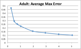
(a)

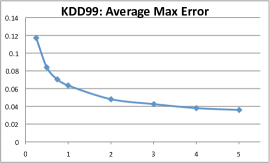
(b)

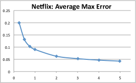
(c)

Figure 2: Average max error of $(\varepsilon,0.001)$-private DualQuery on $500{,}000$ $3$-way marginals versus $\varepsilon$.

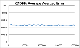
(a)

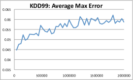
(b)

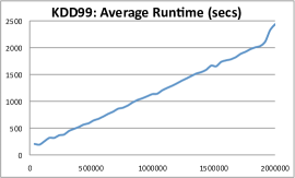
(c)

Figure 3: Error and runtime of $(1,0.001)$-private DualQuery on KDD99 versus number of queries.

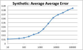
(a)

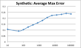
(b)

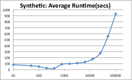
(c)

Figure 4: Error and runtime of $(1,0.001)$-private DualQuery on $100{,}000$ $3$-way marginal queries versus number of attributes.

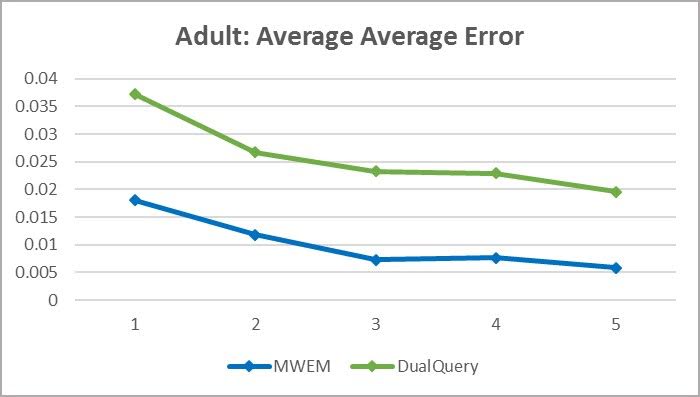
(a)

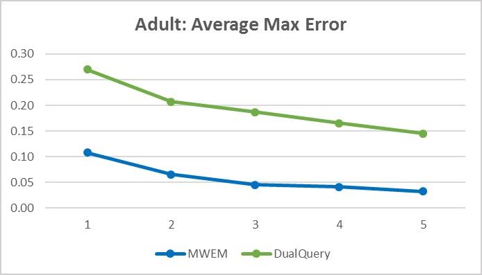
(b)

Figure 5: Comparison of the accuracy performance between DualQuery and MWEM on a low-dimensional dataset with 17 attributes. Both algorithms answer 10,000 queries for the Adult dataset under $(\varepsilon,0)$-differential privacy, where $\varepsilon$ ranges from 1 to 5. In both plots, we show the average and maximum error as a function of the privacy parameter $\varepsilon$.

We evaluate DualQuery on a large collection of $3$-way marginal queries on several real datasets (Figure 1) and high dimensional synthetic data. Adult (census data) and KDD99 (network packet data) are from the UCI repository [2], and have a mixture of discrete (but non-binary) and continuous attributes, which we discretize into binary attributes. We also use the (in)famous Netflix [29] movie ratings dataset, with more than 17,000 binary attributes. More precisely, we can consider each attribute (corresponding to a movie) to be $1$ if a user has watched that movie, and $0$ otherwise.

Rather than set the parameters as in Algorithm 2, we experiment with a range of parameters. For instance, we frequently run for fewer rounds (lower $T$) and take fewer samples (lower $s$). As such, the accuracy guarantee (Theorem 4.6) need not hold for our parameters. However, we find that our algorithm gives good error, often much better than predicted. In all cases, our parameters satisfy the privacy guarantee Theorem 4.3.

We will measure the accuracy of the algorithm using two measures: average error and max error. Given a collection of queries $Q=\{q_{1},\ldots,q_{k}\}$, input database $D$ and the synthetic database $\widehat{D}$ output by our query release algorithm, the average error is defined as

$$\frac{1}{|Q|}\sum_{j}|q_{j}(D)-q_{j}(\widehat{D})|$$

and the max error is defined as

$$\max_{j}|q_{j}(D)-q_{j}(\widehat{D})|.$$

We will run the algorithm multiple times and take the average of both error statistics. While our algorithm uses “negated” $3$-way marginal queries internally, all error figures are for normal, “positive” $3$-way marginal queries only.

Accuracy

We evaluate the accuracy of the algorithm on $500{,}000$ $3$-way marginals on Adult, KDD99 and Netflix. We report maximum error in Figure 2, averaged over $5$ runs. (Marginal queries have range $[0,1]$, so error $1$ is trivial.) Again, all error figures are for normal, “positive” $3$-way marginal queries only. The runs are $(\varepsilon,0.001)$-differentially private, with $\varepsilon$ ranging from $0.25$ to $5$.

For the Adult and KDD99 datasets, we set step size $\eta=2.0$, sample size $s=1000$ while varying the number of steps $T$ according to the privacy budget $\varepsilon$, using the formula from Theorem 4.3. For the Netflix dataset, we adopt the same heuristic except we set $s$ to be $5000$.

The accuracy improves noticeably when $\varepsilon$ increases from $0.25$ to $1$ across 3 datasets, and the improvement diminishes gradually with larger $\varepsilon$. With larger sizes, both KDD99 and Netflix datasets allow DualQuery to run with more steps and get significantly better error.

Scaling to More Queries

Next, we evaluate accuracy and runtime when varying the number of queries. We use a set of $40{,}000$ to $2$ million randomly generated marginals $\mathcal{Q}$ on the KDD99 dataset and run DualQuery with $(1,0.001)$-privacy. For all experiments, we use the same set of parameters: $\eta=1.2,T=170$ and $s=1750$. By Theorem 4.3, each run of the experiment satisfies $(1,0.001)$-differential privacy. These parameters give stable performance as the query class $\mathcal{Q}$ grows. As shown in Figure 3, both average and max error remain mostly stable, demonstrating improved error compared to simpler perturbation approaches. For example, the Laplace mechanism’s error growth rate is $O(\sqrt{|\mathcal{Q}|})$ under $(\varepsilon,\delta)$-differential privacy. The runtime grows almost linearly in the number of queries, since we maintain a distribution over all the queries.

Scaling to Higher Dimensional Data

We also evaluate accuracy and runtime behavior for data dimension ranging from $50$ to $512{,}000$. We evaluate DualQuery under $(1,0.001)$-privacy on $100{,}000$ $3$-way marginals on synthetically generated datasets. We report runtime, max, and average error over $3$ runs in Figure 4; note the logarithmic scale for attributes axis. We do not include query evaluation in our time measurements—this overhead is common to all approaches that answer a set of queries.

When generating the synthetic data, one possibility is to set each attribute to be $0$ or $1$ uniformly at random. However, this generates very uniform synthetic data: a record satisfies any $3$-way marginal with probability $1/8$, so most marginals will have value near $1/8$. To generate more challenging and realistic data, we pick a separate bias $p_{i}\in[0,1]$ uniformly at random for each attribute $i$. For each data point, we then set attribute $i$ to be $1$ independently with probability equal to $p_{i}$. As a result, different $3$-way marginals have different answers on our synthetic data.

For parameters, we fix step size $\eta$ to be $0.4$, and increase the sample size $s$ with the dimension of the data (from $200$ to $50{,}000$) at the expense of running fewer steps. For these parameters, our algorithm is $(1,0.001)$-differentially private by Theorem 4.3. With this set of parameters, we are able to obtain $8\%$ average error in an average of $10$ minutes of runtime, excluding query evaluation.

Comparison with a Simple Baseline

When interpreting our results, it is useful to compare them to a simple baseline solution as a sanity check. Since our real data sets are sparse, we would expect the answer of most queries to be small. A natural baseline is the zeros data set, where all records have all attributes set to $0$.

For the experiments reporting max-error on real datasets, shown in Figure 2, the accuracy of DualQuery out-performs the zeros data set: the zeros data set has a max error of $1$ on both Adult and KDD99 data sets, and a max error of $0.51$ on the Netflix data set. For the experiments reporting average error in Figure 3, the zeros data set also has worse accuracy—it has an average error of $0.11$ on the KDD dataset, whereas DualQuery has an average error below $0.01$.

For synthetic data we can also compare to the zeros dataset, but it is a poor benchmark since the dataset is typically not sparse. Hence, we also compare to a uniform data set containing one of each possible record. Recall that we generate our synthetic data by first selecting a bias $p_{i}$ uniformly at random from $[0,1]$ for each attribute $i$, then setting each record’s attribute $i$ to be $1$ with probability $p_{i}$ (independently across the attributes).

Given this data generation model, we can analytically compute the expected average error on both benchmarks. Consider a query $q$ on literals $a,b,c$. The probability that $q$ evaluates to $1$ on a randomly generated record is $p_{a}\cdot p_{b}\cdot p_{c}$. So, the expected value of $q$ when evaluated on the synthetic data is

$$\mathbb{E}[p_{a}\cdot p_{b}\cdot p_{c}]=0.125$$

since $p_{a},p_{b},p_{c}$ are drawn independently and uniformly from $[0,1]$.

On the zeros data set, $q$ takes value $0$ unless it is of the form $\neg a\land\neg b\land\neg c$, when it takes value $1$. If we average over all queries $q$, this occurs on exactly $1/8$ of the queries. Thus, the expected average error of the zeros database is

$$1/8\cdot\mathbb{E}[1-p_{a}\cdot p_{b}\cdot p_{c}]+7/8\cdot\mathbb{E}[p_{a}\cdot p_{b}\cdot p_{c}]=7/32=0.21875.$$

Similarly, the max-error will tend to $1$ as the size of the data set and number of queries performed grows large. In practice, the max-error in our experiments was above $0.98$.

We can perform a similar calculation with respect the uniform benchmark. Fix any query $q$ on three literals $a,b,$ and $c$. Every query $q$ evaluates to exactly $1/8$ on the uniform benchmark. Thus, the expected error of the uniform benchmark on $q$ is

$$\mathbb{E}[|1/8-p_{a}\cdot p_{b}\cdot p_{c}|],$$

where $p_{a},p_{b},p_{c}$ are drawn independently and randomly from $[0,1]$. This error is

$$\mathbb{E}[|1/8-p_{a}\cdot p_{b}\cdot p_{c}|]=1/256\cdot(7+18\ln 2+2(\ln 8)^{3})\approx 0.11,$$

by a direct calculation.

Similarly, the max-error will tend to $1-1/8=0.875$ as the size of the data set and number of queries performed grows large. In practice, the max-error in our experiments was above $0.85$. Thus, we see that DualQuery outperforms both of these baseline comparisons on synthetic data.

Comparison with MWEM

Finally, we give a brief comparison between the algorithm MWEM of Hardt et al. [20] and DualQuery in terms of the accuracy performance. We tested both algorithms on the Adult dataset with a selection of $17$ attributes to answer $10{,}000$ queries. The accuracy performance of MWEM is better than DualQuery on this low-dimensional dataset (shown in Figure 5). Note that this matches with theoretical guarantees—our theoretical accuracy bounds are worse than MWEM as shown by Hardt and Rothblum [19], Hardt et al. [20]. More generally, for low dimensional datasets for which it is possible to maintain a distribution over records, MWEM likely remains the state of the art. Our work complements MWEM by allowing private data analysis on higher-dimensional data sets. In this experiment, we fix the step size of DualQuery to be $\eta=0.4$, and set the sample size and number of steps to be $(s,T)=(35,47),(40,62),(45,71),(50,78),(55,83)$ to achieve privacy levels of $\varepsilon=1,2,3,4,5$ respectively. For the instantiation of MWEM, we set the number of steps to be $T=15$ (see [20] for more details of the algorithm).

Methodology

In this section, we discuss our experimental setup in more detail.

Implementation details.

The implementation is written in OCaml, using the CPLEX constraint solver. We ran the experiments on a mid-range desktop machine with a 4-core Intel Xeon processor and 12 Gb of RAM. Heuristically, we set a timeout for each CPLEX call to $20$ seconds, accepting the best current solution if we hit the timeout. For the experiments shown, the timeout was rarely reached.

Data discretization.

We discretize KDD99 and Adult datasets into binary attributes by mapping each possible value of a discrete attribute to a new binary feature. We bucket continuous attributes, mapping each bucket to a new binary feature. We also ensure that our randomly generated $3$-way marginal queries are sensible (i.e., they don’t require an original attribute to take two different values).

Setting free attributes.

Since the collection of sampled queries may not involve all of the attributes, CPLEX often finds solutions that leave some attributes unspecified. We set these free attributes heuristically: for real data, we set the attributes to $0$ as these datasets are fairly sparse; for synthetic data, we set attributes to $0$ or $1$ uniformly at random.

Parameter tuning.

DualQuery has three parameters that can be set in a wide variety of configurations without altering the privacy guarantee (Theorem 4.3): number of iterations ($T$), number of samples ($s$), and learning rate ($\eta$), which controls how aggressively to update the distribution. For a fixed level of $\varepsilon$ and $\delta$, there are many feasible private parameter settings.

Performance depends strongly on the choice of parameters: $T$ has an obvious impact—runtime scales linearly with $T$. Other parameters have a more subtle impact on performance—increasing $s$ increases the number of constraints in the integer program for CPLEX, for example. We have investigated a range of parameters, and for the experiments we have used informal heuristics coming from our observations. We briefly describe some of them here. For sparse datasets like the ones in Figure 1, with larger $\eta$ (in the range of 1.5 to 2.0) and smaller $s$ (in the same order as the number of attributes), we obtain good accuracy when we set the free attributes to be $0$. But for denser data like our synthetic data, we get better accuracy when we have smaller $\eta$ (around 0.4) and set the free attributes randomly. As for runtime, we observe that CPLEX could finish running quickly (in seconds) when the sample size is in about the same range as the number of attributes (factor of 2 or 3 different).

Ultimately, our parameters are chosen on a case-by-case basis for each data-set, which is not differentially private. Parameter setting should be done under differential privacy for a truly realistic evaluation (which we do not do). Overall, we do not know of an approach that is both principled and practical to handle this issue end-to-end; private parameter tuning is an area of active research (see e.g., Chaudhuri and Vinterbo [8]).

8 Discussion and conclusion

We have given a new private query release mechanism that can handle datasets with dimensionality multiple orders of magnitude larger than what was previously possible. Indeed, it seems we have not reached the limits of our approach—even on synthetic data with more than $500{,}000$ attributes, DualQuery continues to generate useful answers with about $30$ minutes of overhead on top of query evaluation (which by itself is on the scale of hours). We believe that DualQuery makes private analysis of high dimensional data practical for the first time.

There is still plenty of room for further research. For example, can our approach be improved to match the optimal theoretical accuracy guarantees for query release? We do not know of any fundamental obstacles, but we do not know how to give a better analysis of our current methods. The projection-based approach of Nikolov et al. [30], Dwork et al. [15] seems promising—it achieves theoretically optimal bounds, and like in our approach, the “hard” projection step does not need to be solved privately. It deserves to be studied empirically. On the other hand this approach does not produce synthetic data.

Acknowledgments

We thank Adam Smith, Cynthia Dwork and Ilya Mironov for productive discussions, and for suggesting the Netflix dataset. This work was supported in part by NSF grants CCF-1101389 and CNS-1065060. Marco Gaboardi has been supported by the European Community’s Seventh Framework Programme FP7/2007-2013 under grant agreement No. 272487. This work was partially supported by a grant from the Simons Foundation (#360368 to Justin Hsu).

References

- Arora et al. [2012] Sanjeev Arora, Elad Hazan, and Satyen Kale. The multiplicative weights update method: a meta-algorithm and applications. Theory of Computing, 8(1):121–164, 2012.
- Bache and Lichman [2013] K. Bache and M. Lichman. UCI machine learning repository, 2013.
- Beimel et al. [2013] Amos Beimel, Kobbi Nissim, and Uri Stemmer. Characterizing the sample complexity of private learners. In ACM SIGACT Innovations in Theoretical Computer Science (ITCS), Berkeley, California, pages 97–110, 2013.
- Blum et al. [2013] A. Blum, K. Ligett, and A. Roth. A learning theory approach to noninteractive database privacy. Journal of the ACM, 60(2):12, 2013.
- Blum et al. [2005] Avrim Blum, Cynthia Dwork, Frank McSherry, and Kobbi Nissim. Practical privacy: the sulq framework. In ACM SIGACT–SIGMOD–SIGART Symposium on Principles of Database Systems (PODS), Baltimore, Maryland, pages 128–138, 2005.
- Chaudhuri and Hsu [2011] Kamalika Chaudhuri and Daniel Hsu. Sample complexity bounds for differentially private learning. Journal of Machine Learning Research, 19:155–186, 2011.
- Chaudhuri and Monteleoni [2008] Kamalika Chaudhuri and Claire Monteleoni. Privacy-preserving logistic regression. In Conference on Neural Information Processing Systems (NIPS), Vancouver, British Colombia, pages 289–296, 2008.
- Chaudhuri and Vinterbo [2013] Kamalika Chaudhuri and Staal A. Vinterbo. A stability-based validation procedure for differentially private machine learning. pages 2652–2660, 2013.
- Chaudhuri et al. [2011] Kamalika Chaudhuri, Claire Monteleoni, and Anand D. Sarwate. Differentially private empirical risk minimization. Journal of Machine Learning Research, 12:1069–1109, 2011.
- Chaudhuri et al. [2012] Kamalika Chaudhuri, Anand Sarwate, and Kaushik Sinha. Near-optimal differentially private principal components. In Conference on Neural Information Processing Systems (NIPS), Lake Tahoe, California, pages 998–1006, 2012.
- Duchi et al. [2013] J.C. Duchi, M.I. Jordan, and M.J. Wainwright. Local privacy and statistical minimax rates. In IEEE Symposium on Foundations of Computer Science (FOCS), Berkeley, California, 2013.
- Dwork et al. [2009] C. Dwork, M. Naor, O. Reingold, G.N. Rothblum, and S.P. Vadhan. On the complexity of differentially private data release: efficient algorithms and hardness results. In ACM SIGACT Symposium on Theory of Computing (STOC), Bethesda, Maryland, pages 381–390, 2009.
- Dwork et al. [2010] C. Dwork, G.N. Rothblum, and S. Vadhan. Boosting and differential privacy. In IEEE Symposium on Foundations of Computer Science (FOCS), Las Vegas, Nevada, pages 51––60, 2010.
- Dwork et al. [2006] Cynthia Dwork, Frank McSherry, Kobbi Nissim, and Adam Smith. Calibrating noise to sensitivity in private data analysis. In IACR Theory of Cryptography Conference (TCC), New York, New York, pages 265–284, 2006.
- Dwork et al. [2014] Cynthia Dwork, Aleksandar Nikolov, and Kunal Talwar. Using convex relaxations for efficiently and privately releasing marginals. In SIGACT–SIGGRAPH Symposium on Computational Geometry (SOCG), Kyoto, Japan, page 261, 2014.
- Freund and Schapire [1996] Y. Freund and R.E. Schapire. Game theory, on-line prediction and boosting. In Conference on Computational Learning Theory (CoLT), Desenzano sul Garda, Italy, pages 325–332, 1996.
- Gupta et al. [2012] A. Gupta, A. Roth, and J. Ullman. Iterative constructions and private data release. In IACR Theory of Cryptography Conference (TCC), Taormina, Italy, pages 339–356, 2012.
- Gupta et al. [2013] Anupam Gupta, Moritz Hardt, Aaron Roth, and Jonathan Ullman. Privately releasing conjunctions and the statistical query barrier. SIAM Journal on Computing, 42(4):1494–1520, 2013.
- Hardt and Rothblum [2010] Moritz Hardt and Guy N. Rothblum. A multiplicative weights mechanism for privacy-preserving data analysis. In IEEE Symposium on Foundations of Computer Science (FOCS), Las Vegas, Nevada, pages 61–70, 2010.
- Hardt et al. [2012] Moritz Hardt, Katrina Ligett, and Frank McSherry. A simple and practical algorithm for differentially private data release. In Conference on Neural Information Processing Systems (NIPS), Lake Tahoe, California, pages 2348–2356, 2012.
- Hsu et al. [2013] Justin Hsu, Aaron Roth, and Jonathan Ullman. Differential privacy for the analyst via private equilibrium computation. In ACM SIGACT Symposium on Theory of Computing (STOC), Palo Alto, California, pages 341–350, 2013.
- Kasiviswanathan et al. [2011] Shiva Prasad Kasiviswanathan, Homin K. Lee, Kobbi Nissim, Sofya Raskhodnikova, and Adam Smith. What can we learn privately? SIAM Journal on Computing, 40(3):793–826, 2011.
- Kearns [1998] Michael J. Kearns. Efficient noise-tolerant learning from statistical queries. Journal of the ACM, 45(6):983–1006, 1998.
- Kifer et al. [2012] Daniel Kifer, Adam Smith, and Abhradeep Thakurta. Private convex empirical risk minimization and high-dimensional regression. Journal of Machine Learning Research, 1:41, 2012.
- Li and Miklau [2012] Chao Li and Gerome Miklau. An adaptive mechanism for accurate query answering under differential privacy. volume 5, pages 514–525, 2012.
- Li et al. [2010] Chao Li, Michael Hay, Vibhor Rastogi, Gerome Miklau, and Andrew McGregor. Optimizing linear counting queries under differential privacy. In ACM SIGACT–SIGMOD–SIGART Symposium on Principles of Database Systems (PODS), Indianapolis, Indiana, pages 123–134, 2010.
- McSherry and Talwar [2007] F. McSherry and K. Talwar. Mechanism design via differential privacy. In IEEE Symposium on Foundations of Computer Science (FOCS), Providence, Rhode Island, pages 94–103, 2007.
- Narayanan and Shmatikov [2008] A. Narayanan and V. Shmatikov. Robust de-anonymization of large sparse datasets. In IEEE Symposium on Security and Privacy (S&P), Oakland, California, pages 111–125, 2008.
- [29] Netflix. Netflix prize.
- Nikolov et al. [2013] Aleksandar Nikolov, Kunal Talwar, and Li Zhang. The geometry of differential privacy: the sparse and approximate cases. In ACM SIGACT Symposium on Theory of Computing (STOC), Palo Alto, California, pages 351–360, 2013.
- [31] Aaron Roth and Tim Roughgarden. Interactive privacy via the median mechanism. In ACM SIGACT Symposium on Theory of Computing (STOC), Cambridge, Massachusetts, pages 765–774.
- Rubinstein et al. [2012] Benjamin I. P. Rubinstein, Peter L. Bartlett, Ling Huang, and Nina Taft. Learning in a large function space: Privacy-preserving mechanisms for SVM learning. Journal of Privacy and Confidentiality, 4(1):4, 2012.
- Thakurta and Smith [2013] Abhradeep G. Thakurta and Adam Smith. (Nearly) optimal algorithms for private online learning in full-information and bandit settings. In Conference on Neural Information Processing Systems (NIPS), Lake Tahoe, California, pages 2733–2741, 2013.
- Thaler et al. [2012] Justin Thaler, Jonathan Ullman, and Salil Vadhan. Faster algorithms for privately releasing marginals. In International Colloquium on Automata, Languages and Programming (ICALP), Warwick, England, pages 810–821, 2012.
- Ullman [2013] J. Ullman. Answering counting queries with differential privacy is hard. In ACM SIGACT Symposium on Theory of Computing (STOC), Palo Alto, California, pages 361–370, 2013.
- Ullman and Vadhan [2011] J. Ullman and S.P. Vadhan. PCPs and the hardness of generating private synthetic data. In IACR Theory of Cryptography Conference (TCC), Providence, Rhode Island, pages 400–416, 2011.
- Yaroslavtsev et al. [2013] Grigory Yaroslavtsev, Graham Cormode, Cecilia M. Procopiuc, and Divesh Srivastava. Accurate and efficient private release of datacubes and contingency tables. In IEEE International Conference on Data Engineering (ICDE), Brisbane, Australia, pages 745–756, 2013.
- Zhang et al. [2014] Jun Zhang, Graham Cormode, Cecilia M. Procopiuc, Divesh Srivastava, and Xiaokui Xiao. Privbayes: Private data release via bayesian networks. In ACM SIGMOD International Conference on Management of Data (SIGMOD), Snowbird, Utah, 2014.