Colored noise induces synchronization of limit cycle oscillators

Abstract

Driven by various kinds of noise, ensembles of limit cycle oscillators can synchronize. In this Letter, we propose a general formulation of synchronization of the oscillator ensembles driven by common colored noise with an arbitrary power spectrum. To explore statistical properties of such colored noise-induced synchronization, we derive the stationary distribution of the phase difference between two oscillators in the ensemble. This analytical result theoretically predicts various synchronized and clustered states induced by colored noise and also clarifies that these phenomena have a different synchronization mechanism from the case of white noise.

1 Introduction

Driven by common noise, many nonlinear dynamical systems can synchronize. This phenomenon is called noise-induced synchronization, which is observed in various kinds of the nonlinear dynamical systems, for example, neural networks [1, 2], electric circuits [3], electronic devices [4], microbial cells [5], lasers [6] and chaotic dynamical systems [7, 8]. It has been theoretically proven that limit cycle oscillators can synchronize driven by common noise [9]. Many studies have investigated the synchronization property in case of various types of drive noises, for example, Gaussian white noise [10, 11, 12] and Poisson impulses [13]. In ref. [10], using a formulation of limit cycle oscillators driven by common and independent Gaussian white noises, Nakao et al. analytically obtained the probability density function (PDF) of phase differences between two oscillators, which enables us to effectively characterize the synchronization property. However, although there are some numerical studies[8, 14, 15], analytical conventional studies are limited to the case that drive signals are white noise (temporally uncorrelated noise). If we can assume that the drive signal is white noise, we can use the Fokker-Planck approximation [16] to explore statistical properties of oscillator ensembles. However, such an ideal condition is rare in the real world. For example, in neural circuits, it is known that colored noise with negative autocorrelation plays a key role to propagate synchronous activities [17]. However, it still remains unclear how the oscillators behave if they are driven by common colored noise.

Recently, it has been clarified how a limit cycle oscillator behaves if it is driven by colored non-Gaussian noise [18, 19, 20]. In this Letter, utilizing effective white-noise Langevin description proposed in ref. [19], we extend the formulation in ref. [10] to colored noise that has an arbitrary power spectrum. We then analytically derive the PDF of the phase difference between the oscillators if these oscillators are driven by common colored noise. We also conducted numerical simulations to verify our analytical results. The results show that the PDF of the phase difference explicitly depends on the power spectrum of the drive noise.

2 Model

We used the following system that consists of $N$ identical limit cycle oscillators subject to common and independent multiplicative colored noises. The dynamics of the $j$th oscillator is described by

$$\dot{\bm{X}}^{(j)} = \bm{F}(\bm{X}^{(j)})+\sqrt{D}\bm{G}(\bm{X}^{(j)})\bm{\xi}(t)$$ (1)

$$+\sqrt{\epsilon}\bm{H}(\bm{X}^{(j)})\bm{\eta}^{(j)}(t),$$

for $j=1,\ldots,N$, where $\bm{X}^{(j)}\in\mathbb{R}^{n}$ is the $n$-dimensional state variable of the $j$th oscillator; $\bm{F}(\bm{X}^{(j)})\in\mathbb{R}^{n}$ is an unperturbed vector field that has a stable $T$-periodic limit cycle orbit $\bm{S}(t)$; $\bm{\xi}(t)\in\mathbb{R}^{m}$ is the common noise, which drives all of the oscillators; $\bm{\eta}^{(j)}(t)\in\mathbb{R}^{m}$ ($j=1,\ldots,N$) is the independent noise, which is received independently by each oscillator; $\bm{G}(\bm{X}^{(j)})\in\mathbb{R}^{n\times m}$ and $\bm{H}(\bm{X}^{(j)})\in\mathbb{R}^{n\times m}$ represent how the oscillators are coupled to the common and independent noises; $D$ and $\epsilon$ are parameters to control the intensities of the common and independent noises. We introduced the following three assumptions: (i) $\bm{\xi}(t)\in\mathbb{R}^{m}$ and $\bm{\eta}^{(j)}(t)\in\mathbb{R}^{m}$ are independent, identically distributed zero-mean colored noises, namely, $\langle\bm{\xi}(t)\rangle=\bm{0}$, $\langle\bm{\eta}^{(j)}(t)\rangle=\bm{0}$, $\langle\bm{\xi}(t)\bm{\eta}^{(j)}(s)^{\top}\rangle=\bm{O}$, and $\langle\bm{\eta}^{(j)}(t)\bm{\eta}^{(k)}(s)^{\top}\rangle=\bm{O}$ ($j\neq k$), where $\top$ denotes the transpose and $\langle\cdot\rangle$ represents the temporal average; (ii) $\bm{\xi}(t)$ and $\bm{\eta}^{(j)}(t)$ can be approximated as the convolution of an arbitrary filter function and white noise; and (iii) $\bm{\xi}(t)$ and $\bm{\eta}^{(j)}(t)$ have correlation times shorter than the time scale of the phase diffusion ($\sim O(D^{-\frac{1}{2}},\epsilon^{-\frac{1}{2}})$).

To characterize the statistical properties of the drive noises $\bm{\xi}(t)$ and $\bm{\eta}^{(j)}(t)$, we define correlation matrices $\bm{C}_{\xi}(\tau)\in\mathbb{R}^{m\times m}$ and $\bm{C}_{\eta}(\tau)\in\mathbb{R}^{m\times m}$ as $\bm{C}_{\xi}(\tau)=\langle\bm{\xi}(t)\bm{\xi}(t-\tau)^{\top}\rangle$ and $\bm{C}_{\eta}(\tau)=\langle\bm{\eta}^{(j)}(t)\bm{\eta}^{(j)}(t-\tau)^{\top}\rangle$ ($j=1,\ldots,N$). For the sake of simplicity, we assumed that all independent noises $\bm{\eta}^{(j)}(t)$ have the same statistical property characterized by $\bm{C}_{\eta}(\tau)$. The ($i$, $j$)th element of $\bm{C}_{\xi}(\tau)$ is the cross correlation function of the $i$th and $j$th elements of the common noise $\bm{\xi}(t)$. The diagonal elements of $\bm{C}_{\xi}(\tau)$ are autocorrelation functions. In the same way, we can characterize the statistical property of $\bm{\eta}^{(j)}(t)$ by using $\bm{C}_{\eta}(\tau)$.

3 Phase reduction

Under the assumption that the noise intensity is sufficiently weak ($D\ll 1$ and $\epsilon\ll 1$), we can apply the phase reduction method [21, 20] to eq. (1). By introducing a phase variable $\phi^{(j)}$, eq. (1) is reduced to the following phase equation:

$$\dot{\phi}^{(j)} = \omega+\sqrt{D}\bm{Z}_{\rm G}(\phi^{(j)})\cdot\bm{\xi}(t)$$ (2)

$$+\sqrt{\epsilon}\bm{Z}_{\rm H}(\phi^{(j)})\cdot\bm{\eta}^{(j)}(t)+O(D,\epsilon),$$

where $\phi^{(j)}(t)\in[-\pi,+\pi]$ is a phase variable that corresponds to the state of the $j$th oscillator $\bm{X}^{(j)}$, $\omega$ ($=2\pi T^{-1}$) is the natural frequency, and $\bm{Z}_{G}(\phi^{(j)})$ and $\bm{Z}_{H}(\phi^{(j)})$ are the phase sensitivity functions that represent the linear response of the phase variable $\phi^{(j)}$ to the drive noises[21, 20]. The phase sensitivity functions $\bm{Z}_{G}(\phi^{(j)})$ and $\bm{Z}_{H}(\phi^{(j)})$ are defined as $\bm{Z}_{G}(\phi^{(j)})=\nabla_{\bm{X}}\phi^{(j)}|_{\bm{X}=\bm{S}(\phi^{(j)})}\cdot\bm{G}(\bm{S}(\phi^{(j)}))$ and $\bm{Z}_{H}(\phi^{(j)})=\nabla_{\bm{X}}\phi^{(j)}|_{\bm{X}=\bm{S}(\phi^{(j)})}\cdot\bm{H}(\bm{S}(\phi^{(j)}))$. As discussed in Ref. [20], the $O(D,\epsilon)$ term is necessary to describe the exact phase dynamics, while the phase diffusion is not affected by the $O(D,\epsilon)$ term. As we will focus on the phase diffusion in the following sections, we do not take this term into account.

4 Effective Langevin description

To quantify the synchronization property without loss of generality, we consider the relationship of only two oscillators, that is, the two-body problem of ${\phi}^{(1)}(t)$ and ${\phi}^{(2)}(t)$, and define the phase difference $\theta$ ($:={\phi}^{(1)}-{\phi}^{(2)}$). As we focus on the stochastic dynamics of $\theta$, we define $f(\theta,t)$ as the PDF of the phase difference $\theta$. Utilizing the effective white-noise Langevin description [19], the evolution of $f(\theta,t)$ is described by the following effective Fokker-Planck equation:

$$\frac{\partial f}{\partial t}+\frac{\partial}{\partial\theta}v^{(1)}(\theta)f-\frac{1}{2}\cdot\frac{\partial^{2}}{\partial\theta^{2}}v^{(2)}(\theta)f=0,$$ (3)

where $v^{(1)}(\theta)$ and $v^{(2)}(\theta)$ are effective drift and diffusion coefficients. We have the drift coefficient $v^{(1)}(\theta)=0$ because $\langle\dot{\theta}\rangle=\langle\dot{{\phi}}^{(1)}-\dot{{\phi}}^{(2)}\rangle=0$. Meanwhile, the diffusion coefficient $v^{(2)}(\theta)$ is obtained as

$$v^{(2)}(\theta) = \int_{-\infty}^{+\infty}d\tau\big{\langle}\big{[}\dot{\theta}(t)-\langle\dot{\theta}\rangle\big{]}\big{[}\dot{\theta}(t-\tau)-\langle\dot{\theta}\rangle\big{]}\big{\rangle}$$ (4)

$$= \int_{-\infty}^{+\infty}d\tau\big{\langle}\big{[}\dot{{\phi}}^{(1)}(t)-\dot{{\phi}}^{(2)}(t)\big{]}$$

$$\ \ \big{[}\dot{{\phi}}^{(1)}(t-\tau)-\dot{{\phi}}^{(2)}(t-\tau)\big{]}\big{\rangle}$$

where $\langle\cdot\rangle$ represents the temporal average. For simplicity of notation, we define $d_{jk}$ as $d_{jk}=\int_{-\infty}^{+\infty}d\tau\big{\langle}[\dot{\phi}^{(j)}(t)-\omega][\dot{\phi}^{(k)}(t-\tau)-\omega]\big{\rangle}$. Then, we obtain

$$v^{(2)}(\theta)=d_{11}+d_{22}-d_{12}-d_{21}=2d_{11}-2d_{12}.$$ (5)

The phase variable $\phi^{(j)}(t)$ can be expanded as $\phi^{(j)}(t)=\phi^{(j)}_{0}(t)+\sqrt{D}\phi^{(j)}_{D,1}(t)+\sqrt{\epsilon}\phi^{(j)}_{\epsilon,1}(t)+D\phi^{(j)}_{D,2}(t)+\epsilon\phi^{(j)}_{\epsilon,2}(t)+\cdots$ by using $\sqrt{D}$ and $\sqrt{\epsilon}$ as expansion parameters, where $\phi^{(j)}_{0}(t)$, $\phi^{(j)}_{D,k}(t)$ and $\phi^{(j)}_{\epsilon,k}(t)$ ($k=1,2,\ldots$) are approximate perturbed solutions of $\phi^{(j)}(t)$. We have $\phi^{(j)}_{0}(t)=\phi^{(j)}_{0}(0)+\omega t$, $\dot{\phi}^{(j)}_{D,1}(t)=\bm{Z}_{G}(\phi^{(j)}_{0}(t))\cdot\bm{\xi}(t)$ and $\dot{\phi}^{(j)}_{\epsilon,1}(t)=\bm{Z}_{H}(\phi^{(j)}_{0}(t))\cdot\bm{\eta}^{(j)}(t)$. Using these perturbed solutions, eq. (2) can be written as $\dot{\phi}^{(j)}=\omega+\sqrt{D}\dot{\phi}^{(j)}_{D,1}+\sqrt{\epsilon}\dot{\phi}^{(j)}_{\epsilon,1}+O(D,\epsilon)$. Using this approximation and the fact that $\langle\phi^{(j)}_{D,1}(t)\phi^{(k)}_{\epsilon,1}(t-\tau)\rangle=0$ and $\langle\phi^{(j)}_{\epsilon,1}(t)\phi^{(k)}_{D,1}(t-\tau)\rangle=0$, we obtain

$$d_{jk} = D\int_{-\infty}^{+\infty}d\tau\big{\langle}\dot{\phi}^{(j)}_{D,1}(t)\dot{\phi}^{(k)}_{D,1}(t-\tau)\big{\rangle}$$ (6)

$$+\epsilon\int_{-\infty}^{+\infty}d\tau\big{\langle}\dot{\phi}^{(j)}_{\epsilon,1}(t)\dot{\phi}^{(k)}_{\epsilon,1}(t-\tau)\big{\rangle}$$

$$+O(D^{\frac{3}{2}},\epsilon^{\frac{3}{2}}).$$

Thus, using eq. (6), we can calculate $d_{11}$ as follows:

$$d_{11} = \frac{D}{2\pi}\int_{-\infty}^{+\infty}d\tau\int_{-\pi}^{+\pi}d\phi$$ (7)

$$\ \ \bm{Z}_{G}(\phi)^{\top}\bm{C}_{\xi}(\tau)\bm{Z}_{G}(\phi-\omega\tau)$$

$$+\frac{\epsilon}{2\pi}\int_{-\infty}^{+\infty}d\tau\int_{-\pi}^{+\pi}d\phi$$

$$\ \ \bm{Z}_{H}(\phi)^{\top}\bm{C}_{\eta}(\tau)\bm{Z}_{H}(\phi-\omega\tau)+O(D^{\frac{3}{2}},\epsilon^{\frac{3}{2}}).$$

In the same way, $d_{12}$ is given by

$$d_{12} = \frac{D}{2\pi}\int_{-\infty}^{+\infty}d\tau\int_{-\pi}^{+\pi}d\phi$$ (8)

$$\ \ \bm{Z}_{G}(\phi)^{\top}\bm{C}_{\xi}(\tau)\bm{Z}_{G}(\phi-\theta-\omega\tau)$$

$$+O(D^{\frac{3}{2}},\epsilon^{\frac{3}{2}}).$$

The detailed derivations of eqs. (7) and (8) are shown in Appendix A.

Finally, from eqs. (5), (7) and (8), we have the efficient diffusion coefficient $v^{(2)}(\theta)$:

$$v^{(2)}(\theta)=2D\big{[}g(0)-g(\theta)\big{]}+2\epsilon h(0),$$ (9)

where $g(\theta)$ and $h(\theta)$ are correlation functions defined as

$$g(\theta) = \frac{1}{2\pi}\int_{-\infty}^{+\infty}d\tau\int_{-\pi}^{+\pi}d\phi$$ (10)

$$\ \ \bm{Z}_{G}(\phi)^{\top}\bm{C}_{\xi}(\tau)\bm{Z}_{G}(\phi-\theta-\omega\tau),$$

$$h(\theta) = \frac{1}{2\pi}\int_{-\infty}^{+\infty}d\tau\int_{-\pi}^{+\pi}d\phi$$ (11)

$$\ \ \bm{Z}_{H}(\phi)^{\top}\bm{C}_{\eta}(\tau)\bm{Z}_{H}(\phi-\theta-\omega\tau).$$

If we assume that the drive noise is white, namely, $\bm{C}_{\xi}(\tau)=\bm{C}_{\eta}(\tau)=\delta(\tau)\bm{E}_{m}$, eqs. (10) and (11) are exactly equivalent to eq. (6) in Ref. [10], where $\bm{E}_{m}$ is an $m\times m$ identity matrix. The results show that eqs. (10) and (11) are a natural generalization of eq. (6) in Ref. [10].

We obtain the explicit form of the Fokker-Planck equation of eq. (3) from eqs. (9)–(11). The stationary distribution of the phase difference $f_{0}(\theta)$ is given as the stationary solution of eq. (3). Then, if we put $\partial f/\partial t=0$ in eq. (3), we obtain

$$f_{0}(\theta)=\frac{\nu}{v^{(2)}(\theta)}=\frac{\nu^{\prime}}{D\big{[}g(0)-g(\theta)\big{]}+\epsilon h(0)},$$ (12)

where $\nu$ and $\nu^{\prime}$ ($=\nu/2$) are normalization constants.

5 Fourier representation

To understand the results obtained in the previous section, we rewrite the correlation functions defined in eqs. (10) and (11) by using the Fourier representation. We introduced the Fourier series expansion of the phase sensitivity functions $\bm{Z}_{G}(\phi)$ and $\bm{Z}_{H}(\phi)$ as $\bm{Z}_{G}(\phi)=\sum_{l=-\infty}^{+\infty}\bm{Y}_{G,l}e^{il\phi}$ and $\bm{Z}_{H}(\phi)=\sum_{l=-\infty}^{+\infty}\bm{Y}_{H,l}e^{il\phi}$ , where $i$ denotes the imaginary unit and $\bm{Y}_{G,l}\in\mathbb{C}^{m}$ ($=\frac{1}{2\pi}\int_{-\pi}^{+\pi}d\phi\bm{Z}_{G}(\phi)e^{-il\phi}$) and $\bm{Y}_{H,l}\in\mathbb{C}^{m}$ ($=\frac{1}{2\pi}\int_{-\pi}^{+\pi}d\phi\bm{Z}_{H}(\phi)e^{-il\phi}$) are Fourier coefficients ($l=-\infty,\ldots,\infty$).

Subsequently, we define $\bm{P}_{\xi}(\Omega)\in\mathbb{C}^{m\times m}$ and $\bm{P}_{\eta}(\Omega)\in\mathbb{C}^{m\times m}$ as the Fourier transforms of $\bm{C}_{\xi}(\tau)$ and $\bm{C}_{\eta}(\tau)$, that is, $\bm{P}_{\xi}(\Omega)=\int_{-\infty}^{+\infty}dt\bm{C}_{\xi}(t)e^{-i\Omega t}$ and $\bm{P}_{\eta}(\Omega)=\int_{-\infty}^{+\infty}dt\bm{C}_{\eta}(t)e^{-i\Omega t}$. Let us note that $\bm{P}_{\xi}(\Omega)$ and $\bm{P}_{\eta}(\Omega)$ are Hermitian matrices, namely, $\bm{P}_{\xi}(\Omega)=\bm{P}_{\xi}(\Omega)^{{\dagger}}$ and $\bm{P}_{\eta}(\Omega)=\bm{P}_{\eta}(\Omega)^{{\dagger}}$ because $\bm{C}_{\xi}(\tau)=\bm{C}_{\xi}(-\tau)^{\top}$ and $\bm{C}_{\eta}(\tau)=\bm{C}_{\eta}(-\tau)^{\top}$ from their definitions, where ${\dagger}$ denotes the adjoint. The $(i,j)$th elements of $\bm{P}_{\xi}(\Omega)$ and $\bm{P}_{\eta}(\Omega)$ represent the cross spectra of the $i$th and $j$th elements of $\bm{\xi}(t)$ and $\bm{\eta}^{(j)}(t)$. In particular, the diagonal elements of $\bm{P}_{\xi}(\Omega)$ and $\bm{P}_{\eta}(\Omega)$ represent the power spectra.

Using the Fourier representations defined above, we can obtain the Fourier representations of the correlation functions $g(\theta)$ and $h(\theta)$:

$$g(\theta)=\sum_{l=-\infty}^{+\infty}g_{l}e^{il\theta},\ h(\theta)=\sum_{l=-\infty}^{+\infty}h_{l}e^{il\theta},$$ (13)

where $g_{l}$ ($=\bm{Y}_{G,l}^{{\dagger}}\bm{P}_{\xi}(l\omega)\bm{Y}_{G,l}$) and $h_{l}$ ($=\bm{Y}_{H,l}^{{\dagger}}\bm{P}_{\eta}(l\omega)\bm{Y}_{H,l}$) are Fourier coefficients ($l=-\infty,\ldots,\infty$). The derivations of $g_{l}$ and $h_{l}$ will be shown in Appendix B.

These expressions clearly suggest that the correlation functions $g(\theta)$ and $h(\theta)$ only depend on $\bm{P}_{\xi}(\pm l\omega)$ and $\bm{P}_{\eta}(\pm l\omega)$ ($l=0,1,2,\ldots$), that is, the other frequency components can be neglected. In the next section, we will demonstrate that colored noise induces various synchronized and clustered states, which are clearly explained by eq. (13).

6 Numerical simulations

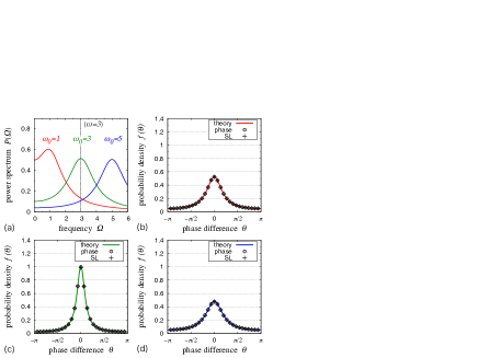
Figure 1: (Color online) Simulation results of the Stuart-Landau oscillator (crosses) and the corresponding phase oscillator (open circles). (a) Power spectra of the common noises are shown for $\omega_{0}=1$, 3 and 5. The PDFs of $\theta$ show the frequency dependency of the synchronization property for (b) $\omega_{0}=1$, (c) $\omega_{0}=3$ ($=\omega$), and (d) $\omega_{0}=5$.

To demonstrate the validity of our results, we perform numerical experiments for two types of limit cycle oscillators. The first example is the Stuart-Landau oscillator, which takes the normal form of the supercritical Hopf bifurcation [21]: $\dot{x}=x-c_{0}y-(x^{2}+y^{2})(x-c_{2}y)$, $\dot{y}=y+c_{0}x-(x^{2}+y^{2})(y+c_{2}x)$, where $\bm{X}=[x,y]^{\top}$ is a state variable and $c_{0}$ and $c_{2}$ are parameters. In the simulation, we fixed $c_{0}=1$, $c_{2}=-2$, $\bm{G}=\bm{H}={\rm diag}(1,1)$, $D=0.0095$ and $\epsilon=0.0005$, where ${\rm diag}(\lambda_{1},\ldots,\lambda_{m})$ denotes an $m\times m$ diagonal matrix that has the diagonal elements $\lambda_{1},\ldots,\lambda_{m}$. This model is reduced to the phase equation that has the natural frequency $\omega=c_{0}-c_{2}=3$ and the phase sensitivity function $\bm{Z}(\phi)=\sqrt{2}[\sin(\phi+3\pi/4),\sin(\phi+\pi/4)]^{\top}$.

In the simulation, we use a two-dimensional drive noise that has the correlation matrix $\bm{C}_{\rm ex}(\tau)\in\mathbb{R}^{2\times 2}$ defined as $\bm{C}_{\rm ex}(\tau)={\rm diag}(C_{\rm ex}(\tau),C_{\rm ex}(\tau))$ and $C_{\rm ex}(\tau)=\frac{\gamma}{2}e^{-\gamma|\tau|}\cos\omega_{0}\tau$, where $\omega_{0}$ and $\gamma$ are parameters that represent the peak frequency and the characteristic decay time. We define $P_{\rm ex}(\Omega)$, the Fourier transform of $C_{\rm ex}(\tau)$, as $P_{\rm ex}(\Omega)=\frac{\gamma^{2}}{2}\{[\gamma^{2}+(\Omega+\omega_{0})^{2}]^{-1}+[\gamma^{2}+(\Omega-\omega_{0})^{2}]^{-1}\}$. A drive noise characterized by $C_{\rm ex}(\tau)$ can be generated by the damped noisy harmonic oscillator (See eqs. (43)–(49) in Ref. [19] for details).

We use the common noises with $(\omega_{0},\gamma)=(1,1)$, $(3,1)$ and $(5,1)$ and the independent noise with $(\omega_{0},\gamma)=(0,3)$. The power spectra of these common noises are shown in fig. 1 (a). From eq. (13), the correlation functions $g(\theta)$ and $h(\theta)$ are given by $g(\theta)=\{[1+(\omega_{0}+3)^{2}]^{-1}+[1+(\omega_{0}-3)^{2}]^{-1}\}\cos\theta$ and $h(\theta)=\cos\theta$, for $\omega_{0}=$ 1, 3 and 5, which correspond to the three types of the common noise. The derivations of $g(\theta)$ and $h(\theta)$ will be shown in Appendix C.

The correlation function $g(\theta)$ calculated above indicate that the effective intensity of the common noise depends on the peak frequency $\omega_{0}$ and is maximal at $\omega_{0}=\omega$. It means that the synchronous degree is maximized at $\omega_{0}=\omega$. In fig. 1 (b)–(d), we compared the results of the direct numerical simulation using the Stuart-Landau oscillator and its corresponding phase oscillator with the analytical results. All PDFs are well fitted by the theoretical curves. Our theory clearly predicts that the highest synchronous degree is realized at $\omega_{0}=\omega$.

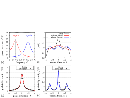
Figure 2: (Color online) Simulation results of the FitzHugh-Nagumo oscillator. (a) Power spectra of the common noises are shown for $\omega_{0}=\omega$ and $3\omega$. For these drive noises, (b) $g(\theta)$ ($=h(\theta)$) is shown. The PDFs of $\theta$ for (c) $\omega_{0}=\omega$ (synchronized state) and for (d) $\omega_{0}=3\omega$ (3-cluster state) are shown.

The second example is the FitzHugh-Nagumo oscillator [22, 23]: $\dot{v}=v-v^{3}/3-u+I_{0}$, $\dot{u}=\mu(v+a-bu)$, where $\bm{X}=[v,u]^{\top}$ is a state variable and $a$, $b$, $\mu$ and $I_{0}$ are parameters. In the simulation, we fixed $a=0.7$, $b=0.8$, $\mu=0.08$, $I_{0}=0.875$, $\bm{G}=\bm{H}={\rm diag}(1,0)$, $D=0.045$ and $\epsilon=0.005$. For these parameters, this oscillator has the natural frequency $\omega\simeq 0.1725$. This oscillator models bursting behavior of a neuron, and only the first variable $v$, which corresponds to the membrane potential of a neuron, is subject to noise.

In the simulation, we use the one-dimensional noise that has the correlation function $C_{\rm ex}(\tau)$. Different from the first example, we use the same parameters $(\omega_{0},\gamma)$ for both the common and independent noises. We used two parameter sets $(\omega_{0},\gamma)=(\omega,0.1)$ and $(3\omega,0.1)$. The power spectra of these drive noises are shown in fig. 2 (a). We obtain the correlation function $g(\theta)$ ($=h(\theta)$) numerically as shown in fig. 2 (b).

In fig. 2 (c) and (d), we compared the results of the direct numerical simulation with the analytical results. The numerical results are in good agreement with the theoretical results. As theoretically predicted, a 3-cluster state is realized as shown in fig. 2 (d). If oscillators are driven by white noise, clustered states are induced only by multiplicative noise [10]. However, in case of colored noise, clustered states are induced not only by multiplicative noise but also by additive noise.

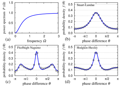
Figure 3: (Color online) Simulation results of the limit cycle oscillators subject to green noise. (a) Power spectra of the drive noises. The PDFs of $\theta$ obtained by the theory (lines) and numerical simulations (circles) for (b) the Stuart-Landau oscillator, (c) the FitzHugh-Nagumo oscillator and (d) the Hodgkin-Huxley oscillator.

In the third example, we used the Hodgkin-Huxley oscillator[25], which enables us to demonstrate whether the theory is applicable to higher-dimensional limit cycle systems. We use green noise used in ref. [8], which is generated by applying a high-pass filter to white noise. The power spectrum is shown in fig. 3 (a). Different from the periodic noise characterized by $C_{\rm ex}(\tau)$, the green noise has a vanishing spectrum as $\Omega\to 0$. In the simulation, for the sake of simplicity, we used the same type of drive noise for the common and independent noises, and we set the noise intensities $(D,\epsilon)=(0.0002,0.0001)$. Fig. 3 (b)–(d) compare the theoretical and numerical results, which show that our theory is also valid for these cases.

7 Summary and discussions

In this Letter, we extended a formulation to analyze various synchronized and clustered states of uncoupled limit cycle oscillators driven by common and independent colored noises. Using this formulation, we derived the probability density function of the phase difference and rewrote it by the Fourier representation. The obtained expressions clearly show that the synchronization property depends on the power spectrum of the drive noises. Such dependency has already been reported experimentally. For example, in ref. [24], the reliability, or synchronization across trials, is explored in neuronal responses to periodic drive inputs with various frequencies. The reliability is maximized at a certain frequency, which is similar to our results shown in fig. 1. Our results in this Letter supports the results in ref. [24] theoretically, because a neuron in a oscillatory state can be regarded as a noisy limit cycle oscillator.

Generally, noise in the real world often has a non-flat and characteristic power spectrum. In this sense, our formulation is a useful tool to estimate the synchronization property for both theoretical and practical aspects. Namely, the results obtained in this Letter can be applied to a wide range of purposes from mathematical modelings to technological problems.

8 Appendix A: Derivations of eqs. (7) and (8)

Substituting $\dot{\phi}_{D,1}^{(j)}=\bm{Z}_{G}(\phi_{0}^{(j)}(t))\cdot\bm{\xi}(t)$ and $\dot{\phi}_{\epsilon,1}^{(j)}=\bm{Z}_{H}(\phi_{0}^{(1)}(t))\cdot\bm{\eta}^{(1)}(t)$ into eq. (6), we obtain

$$d_{11} = D\int_{-\infty}^{+\infty}d\tau\big{\langle}[\bm{Z}_{G}(\phi_{0}^{(1)}(t))^{\top}\bm{\xi}(t)]$$ (A.2 )

$$\ \ [\bm{Z}_{G}(\phi_{0}^{(1)}(t-\tau))^{\top}\bm{\xi}(t-\tau)]\big{\rangle}$$

$$+\epsilon\int_{-\infty}^{+\infty}d\tau\big{\langle}[\bm{Z}_{H}(\phi_{0}^{(1)}(t))^{\top}\bm{\eta}^{(1)}(t)]$$

$$\ \ [\bm{Z}_{H}(\phi_{0}^{(1)}(t-\tau))^{\top}\bm{\eta}^{(1)}(t-\tau)]\big{\rangle}$$

$$+O(D^{\frac{3}{2}},\epsilon^{\frac{3}{2}})$$

$$= D\int_{-\infty}^{+\infty}d\tau\big{\langle}\bm{Z}_{G}(\phi_{0}^{(1)}(t))^{\top}\bm{\xi}(t)$$

$$\ \ \bm{\xi}(t-\tau)^{\top}\bm{Z}_{G}(\phi_{0}^{(1)}(t-\tau))\big{\rangle}$$

$$+\epsilon\int_{-\infty}^{+\infty}d\tau\big{\langle}\bm{Z}_{H}(\phi_{0}^{(1)}(t))^{\top}\bm{\eta}^{(1)}(t)$$

$$\ \ \bm{\eta}^{(1)}(t-\tau)^{\top}\bm{Z}_{H}(\phi_{0}^{(1)}(t-\tau))\big{\rangle}$$

$$+O(D^{\frac{3}{2}},\epsilon^{\frac{3}{2}}).$$

We rewrite $\bm{Z}_{G}(\phi)$, $\bm{Z}_{H}(\phi)$, $\bm{\xi}(t)$ and $\bm{\eta}^{(1)}(t)$ by using their elements and obtain

$$d_{11} = D\int_{-\infty}^{+\infty}d\tau\sum_{k=1}^{m}\sum_{l=1}^{m}\big{\langle}Z_{H,k}(\phi_{0}^{(1)}(t))$$ (A.3 )

$$\ \ \xi_{k}(t)\xi_{l}(t-\tau)Z_{H,l}(\phi_{0}^{(1)}(t-\tau))\big{\rangle}$$

$$+\epsilon\int_{-\infty}^{+\infty}d\tau\ \sum_{k=1}^{m}\sum_{l=1}^{m}\big{\langle}Z_{H,k}(\phi_{0}^{(1)}(t))$$

$$\ \ \eta^{(1)}_{k}(t)\eta^{(1)}_{l}(t-\tau)Z_{H,l}(\phi_{0}^{(1)}(t-\tau))\big{\rangle}$$

$$+O(D^{\frac{3}{2}},\epsilon^{\frac{3}{2}}),$$

where $Z_{G,l}(\phi)$ and $Z_{H,l}(\phi)$ are the $l$th elements of $\bm{Z}_{G}(\phi)$ and $\bm{Z}_{H}(\phi)$, and $\xi_{l}(t)$ and $\eta_{l}^{(1)}(t)$ are the $l$th elements of $\bm{\xi}(t)$ and $\bm{\eta}^{(1)}(t)$.

We assume that the phase variable $\phi^{(1)}$ and the drive noises $\bm{\xi}(t)$ and $\bm{\eta}^{(1)}(t)$ are approximately independent. Under this assumption, the temporal average $\langle\cdot\rangle$ can be divided into two parts; $\langle\cdot\rangle_{\phi}$ ($:=(2\pi)^{-1}\int_{-\pi}^{+\pi}d\phi\,\cdot\,$) and $\langle\cdot\rangle_{t}$ ($:=\lim_{s\to\infty}(2s)^{-1}\int_{-s}^{+s}dt\,\cdot\,$). Thus, we obtain

$$d_{11} = D\int_{-\infty}^{+\infty}d\tau\sum_{k=1}^{m}\sum_{l=1}^{m}\big{\langle}Z_{G,k}(\phi_{0}^{(1)}(t))$$ (A.4 )

$$\ \ Z_{G,l}(\phi_{0}^{(1)}(t-\tau))\big{\rangle}_{\phi}\big{\langle}\xi_{k}(t)\xi_{l}(t-\tau)\big{\rangle}_{t}$$

$$+\epsilon\int_{-\infty}^{+\infty}d\tau\ \sum_{k=1}^{m}\sum_{l=1}^{m}\big{\langle}Z_{H,k}(\phi_{0}^{(1)}(t))$$

$$\ \ Z_{H,l}(\phi_{0}^{(1)}(t-\tau))\big{\rangle}_{\phi}\big{\langle}\eta^{(1)}_{k}(t)\eta^{(1)}_{l}(t-\tau)\big{\rangle}_{t}$$

$$+O(D^{\frac{3}{2}},\epsilon^{\frac{3}{2}})$$

$$= \frac{D}{2\pi}\int_{-\infty}^{+\infty}d\tau\int_{-\pi}^{+\pi}d\phi$$

$$\ \ \sum_{k=1}^{m}\sum_{l=1}^{m}Z_{G,k}(\phi)Z_{G,l}(\phi-\omega\tau)C_{\xi,kl}(\tau)$$

$$+\frac{\epsilon}{2\pi}\int_{-\infty}^{+\infty}d\tau\ \int_{-\pi}^{+\pi}d\phi$$

$$\ \ \sum_{k=1}^{m}\sum_{l=1}^{m}Z_{H,k}(\phi)Z_{H,l}(\phi-\omega\tau)C_{\eta,kl}(\tau)$$

$$+O(D^{\frac{3}{2}},\epsilon^{\frac{3}{2}}),$$

where $C_{\xi,kl}$ and $C_{\eta,kl}$ are the $(k,l)$th elements of $\bm{C}_{\xi}(\phi)$ and $\bm{C}_{\eta}(\phi)$. Finally, we rewrite eq. (A.4) by using $\bm{Z}_{G}(\phi)$, $\bm{Z}_{H}(\phi)$, $\bm{C}_{\xi}(\tau)$ and $\bm{C}_{\eta}(\tau)$ and obtain

$$d_{11} = \frac{D}{2\pi}\int_{-\infty}^{+\infty}d\tau\int_{-\pi}^{+\pi}d\phi$$ (A.5 )

$$\ \ \bm{Z}_{G}(\phi)^{\top}\bm{C}_{\xi}(\tau)\bm{Z}_{G}(\phi-\omega\tau)$$

$$+\frac{\epsilon}{2\pi}\int_{-\infty}^{+\infty}d\tau\int_{-\pi}^{+\pi}d\phi$$

$$\ \ \bm{Z}_{H}(\phi)^{\top}\bm{C}_{\eta}(\tau)\bm{Z}_{H}(\phi-\omega\tau)$$

$$+O(D^{\frac{3}{2}},\epsilon^{\frac{3}{2}}).$$

In the same way, one can calculate $d_{12}$ as follows. We use the fact that $\langle\phi^{(1)}_{\epsilon,1}(t)\phi^{(2)}_{\epsilon,1}(t-\tau)\rangle=0$ and eliminate the phase variable of the second oscillator $\phi^{(2)}_{0}$ by substituting $\phi^{(2)}_{0}=\phi^{(1)}_{0}-\theta$ into $\phi^{(2)}_{0}$, and then, we obtain

$$d_{12} = D\int_{-\infty}^{+\infty}d\tau\big{\langle}[\bm{Z}_{G}(\phi_{0}^{(1)}(t))^{\top}\bm{\xi}(t)]$$ (A.6 )

$$\ \ [\bm{Z}_{G}(\phi_{0}^{(2)}(t-\tau))^{\top}\bm{\xi}(t-\tau)]\big{\rangle}$$

$$+O(D^{\frac{3}{2}},\epsilon^{\frac{3}{2}})$$

$$= D\int_{-\infty}^{+\infty}d\tau\big{\langle}\bm{Z}_{G}(\phi_{0}^{(1)}(t))^{\top}\bm{\xi}(t)$$

$$\ \ \bm{\xi}(t-\tau)^{\top}\bm{Z}_{G}(\phi_{0}^{(2)}(t-\tau))\big{\rangle}$$

$$+O(D^{\frac{3}{2}},\epsilon^{\frac{3}{2}})$$

$$= \frac{D}{2\pi}\int_{-\infty}^{+\infty}d\tau\int_{-\pi}^{+\pi}d\phi$$

$$\ \ \bm{Z}_{G}(\phi)^{\top}\bm{C}_{\xi}(\tau)\bm{Z}_{G}(\phi-\theta-\omega\tau)$$

$$+O(D^{\frac{3}{2}},\epsilon^{\frac{3}{2}}).$$

9 Appendix B: Derivation of eq. (13)

From eq. (10), one can calculate the Fourier coefficient $g_{l}$ as follows. We introduce a new variable $\chi$ ($:=\phi-\theta-\omega\tau$) and use the fact that $\bm{P}_{\xi}(\Omega)$ is a Hermitian matrix. Then, we obtain

$$g_{l} = \frac{1}{2\pi}\int_{-\pi}^{+\pi}d\theta g(\theta)e^{-il\theta}$$ (B.1 )

$$= \frac{1}{2\pi}\int_{-\pi}^{+\pi}d\theta\frac{1}{2\pi}\int_{-\infty}^{+\infty}d\tau\int_{-\pi}^{+\pi}d\phi\bm{Z}_{G}(\phi)^{\top}$$

$$\ \ \bm{C}_{\xi}(\tau)\bm{Z}_{G}(\phi-\theta-\omega\tau)e^{-il\theta}$$

$$= \bigg{(}\frac{1}{2\pi}\int_{-\pi}^{+\pi}d\phi\bm{Z}_{G}(\phi)^{\top}e^{-il\phi}\bigg{)}$$

$$\bigg{(}\int_{-\infty}^{+\infty}d\tau\bm{C}_{\xi}(\tau)e^{il\omega\tau}\bigg{)}\bigg{(}\frac{1}{2\pi}\int_{-\pi}^{+\pi}d\chi\bm{Z}_{G}(\chi)e^{il\chi}\bigg{)}$$

$$= \bm{Y}_{G,l}^{\top}\overline{\bm{P}_{\xi}(l\omega)}\,\overline{\bm{Y}_{G,l}}=\bm{Y}_{G,l}^{{\dagger}}\bm{P}_{\xi}(l\omega)^{{\dagger}}\bm{Y}_{G,l}$$

$$= \bm{Y}_{G,l}^{{\dagger}}\bm{P}_{\xi}(l\omega)\bm{Y}_{G,l},$$

where $\overline{\ \cdot\ }$ denotes the complex conjugate. From eq. (11), $h_{l}$ can be derived likewise.

10 Appendix C: Derivations of the correlation functions $g(\theta)$ and $h(\theta)$

For the Stuart-Landau oscillator we used in the simulations, we can calculate the Fourier coefficients $\bm{Y}_{G,l}$ and $\bm{Y}_{H,l}$ as $\bm{Y}_{G,\pm 1}=\bm{Y}_{H,\pm 1}=\frac{1}{2}[1\pm i,1\mp i]^{\top}$ and $\bm{Y}_{G,l}=\bm{Y}_{H,l}=\bm{0}\ (l\neq\pm 1)$. Thus, from eq. (13), the Fourier coefficient $g_{l}$ is given by $g_{\pm 1}=\bm{Y}_{G,\pm l}^{{\dagger}}\bm{Y}_{G,\pm l}P_{\rm ex}(\omega)|_{\gamma=1}=\frac{1}{2}\{[1+(\omega_{0}+3)^{2}]^{-1}+[1+(\omega_{0}-3)^{2}]^{-1}\}$ and $g_{l}=0\ \ (l\neq\pm 1)$, where $\omega_{0}$ is a parameter. In the same way, the Fourier coefficient $h_{l}$ is given by $h_{\pm 1}=\bm{Y}_{H,\pm l}^{{\dagger}}\bm{Y}_{H,\pm l}P_{\rm ex}(\omega)|_{\omega_{0}=0,\gamma=3}=\frac{1}{2}$ and $h_{l}=0\ \ (l\neq\pm 1)$. Substituting $g_{l}$ and $h_{l}$ to eq. (13), we can obtain the explicit forms of $g(\theta)$ and $h(\theta)$.

References

[1]\NameMainen Z. F. Sejnowski T. J. \REVIEWScience26819951503.
[2]\NameGalán R. F., Fourcaud-Trocmé N., Ermentrout G. B. Urban N. N.
\REVIEWJ. Neurosci.2620063646.
[3]\NameYoshida K., Sato K. Sugamata A. \REVIEWJ. Sound Vib.290200634.
[4]\NameUtagawa A., Asai T., Hirose T. Amemiya Y. \REVIEWIEICE Trans.
Fundam.9120082475.
[5]\NameZhou T., Chen L. Aihara K. \REVIEWPhys. Rev. Lett.952005178103.
[6]\NameUchida A., McAllister R. Roy R. \REVIEWPhys. Rev. Lett.932004244102.
[7]\NameZhou C. Kurths J. \REVIEWPhys. Rev. Lett.882002230602.
[8]\NameWang Y., Lai Y.-C., Zheng Z.\REVIEWPhys. Rev. E792009056210.
[9]\NameTeramae J.-N. Tanaka D. \REVIEWPhys. Rev. Lett.932004204103.
[10]\NameNakao H., Arai K. Kawamura Y. \REVIEWPhys. Rev. Lett.982007184101.
[11]\NameYoshimura K., Davis P. Uchida A. \REVIEWProg. Theor. Phys.1202008621.
[12]\NameNagai K. H. Kori H. \REVIEWPhys. Rev. E812010065202.
[13]\NameNakao H., Arai K., Nagai K., Tsubo Y. Kuramoto Y. \REVIEWPhysical
Review E72200526220.
[14]\NameYoshimura K., Valiusaityte I. Davis P. \REVIEWPhys. Rev. E752007026208.
[15]\NameHata S., Shimokawa T., Arai K. Nakao H. \REVIEWPhys. Rev. E822010036206.
[16]\NameRisken H. \BookThe Fokker-Planck equation: Methods of solution and
applications (Springer Verlag) 1996.
[17]\NameCâteau H. Reyes A. D. \REVIEWPhys. Rev. Lett.962006058101.
[18]\NameTeramae J. Tanaka D. \REVIEWProg. Theor. Phys.1612006360.
[19]\NameNakao H., Teramae J.-N., Goldobin D. S. Kuramoto Y. \REVIEWChaos2020103126.
[20]\NameGoldobin D. S., Teramae J.-N., Nakao H. Ermentrout G. B.
\REVIEWPhys. Rev. Lett.1052010154101.
[21]\NameKuramoto Y. \BookChemical oscillations, waves, and turbulence (Dover
Publications) 2003.
[22]\NameFitzHugh R.
\REVIEWBiophys. J.11961445.
[23]\NameNagumo J., Arimoto S. Yoshizawa S.
\REVIEWProc. IRE5019622061.
[24]\NameFellous J. M., Houweling A. R., Modi R. H., Rao R. P. N., Tiesinga
P. H. E. Sejnowski T. J. \REVIEWJ. Neurophysiol.8520011782.
[25]\NameHodgkin A. Huxley A. \REVIEWJ. Physiol.1171952500.