An empirical model for $pp$ scattering and geometrical scaling

Abstract

We present the result of an empirical model for elastic $pp$ scattering at LHC which indicates that the asymptotic black disk limit ${\cal R}=\sigma_{elastic}/\sigma_{total}\rightarrow 1/2$ is not yet reached and discuss the implications on classical geometrical scaling behavior. We propose a geometrical scaling law for the position of the dip in elastic $pp$ scattering which allows to make predictions valid both for intermediate and asymptotic energies.

1 An empirical model for $pp$ scattering

The measurements of the total and differential elastic $pp$ cross-section at LHC at $\sqrt{s}=7\ TeV$ (LHC7) [1] and $\sqrt{s}=8\ TeV$ (LHC8) [2] have presented, once more, the question of asymptotic behavior in hadron-hadron scattering [3, 4]. In this note, we shall discuss this behavior through the results of an empirical model for the elastic amplitude, [3], i.e.

$$\mathcal{A}(s,t)=i[G(s,t)\sqrt{A(s)}e^{B(s)t/2}+e^{i\phi(s)}\sqrt{C(s)}e^{D(s)t/2}].$$ (1)

The above expression for the case $G(s,t)\equiv 1$ gives the well known Barger and Philips (“model independent”) parametrization proposed in [5], which reproduces very well the $-t$-region before, at, and after the dip, from ISR to LHC, except for what concerns the $-t\approx 0$ behavior. This model fails to reproduce with good accuracy the optical point, i.e. the total cross section. The description was improved through a modification of Eq. (1) which incorporated the proton e.m. form factor, namely

$$G(s,t)=F^{2}_{P}(t)=1/(1-t/t_{0})^{4}$$ (2)

With all the parameters in Eqs.  (1, 2) as free parameters, the resulting analysis of elastic $pp$ data from ISR to LHC7 is shown in Fig. 1. In this figure, the right hand panel includes a comparison with a parametrization of the tail of the distribution given by the TOTEM collaboration (dotted line). Such parametrization, $(-t)^{-8}$, was suggested in [6], and recently proposed again in [7], where it is shown to describe large $-t$ data from ISR to LHC8, and for both $pp$ and $\bar{p}p$, whenever available. The proposed behaviour is independent of energy in the common range of momentum transfer, is purely real, and arising from a 3-gluon exchange term with $C=-1$. Work to incorporate such behaviour in the present empirical model is under consideration.

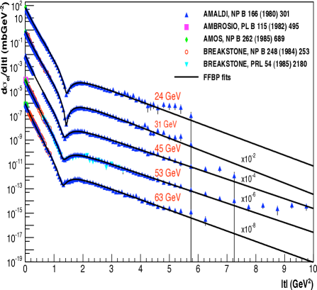
Figure 1: Fits to the ISR and LHC7 data sets with model of Eqs. (1,2) (labeled FFBP in the frame), with $t_{0}$ a free parameter. Data sets and parameter values for ISR data can be found in [3]. Inset: LHC7 data near the optical point are shown in comparison with the present model, which includes the proton form factor modification. Figure is from [3].

From our fits with the empirical model of Eqs. (1,2), we extract the elastic profile, through the Hankel transform of the amplitude Eqs. (1, 2):

$$A_{el}(s,b)=-i\int_{0}^{\infty}qdqJ_{0}(qb)\mathcal{A}(s,t).$$ (3)

This amplitude in $b-$ space is shown in Fig.  2.

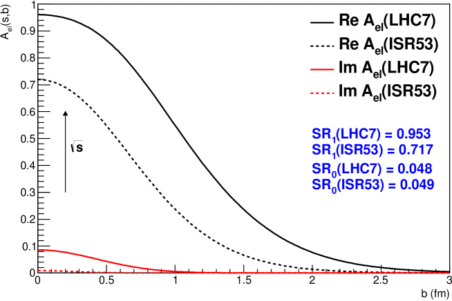
Figure 2: Imaginary and real parts of the Hankel transform of the amplitude obtained with the empirical model of Eqs. (1,2) from parameter values as in [3]. The values of two sum rules for the amplitude, $SR_{1}$ and $SR_{0}$, also from [3] are displayed for the c.m energies 7 TeV and 53 GeV.

The energy dependence of the 6 free parameters, two amplitudes $A(s),\ C(s)$, two slopes $B(s),\ D(s)$, a phase $\phi$ and the scale $t_{0}$, is a priori unknown, although an interpretation in terms of a Regge model can be obtained [8]. However, maintaining a model independent point of view, we have resorted to asymptotic theorems to make an ansatz concerning the energy dependence of the parameters. We have proposed the following energy behavior:

$$4\sqrt{\pi A(s)}(mb)=47.8-3.8\ln s+0.398(\ln s)^{2}$$ (4)

$$B(s)(GeV^{-2})=1.04+0.028(\ln s)^{2}-\frac{8}{0.71}=-0.23+0.028(\ln s)^{2}$$ (5)

$$4\sqrt{\pi C(s)}(mb)=\frac{9.6-1.8\ln s+0.01(\ln s)^{3}}{1.2+0.001(\ln s)^{3}}$$ (6)

$$D(s)(GeV^{-2})=-0.41+0.29\ln s$$ (7)

The parametrization for $C(s)$ is empirical, $\sqrt{A(s)}$ and $B(s)$ follow asymptotic maximal energy saturation behavior of the total cross-section (Froissart limit), $D(s)$ shows normal Regge behavior. The scale in the logarithmic terms is understood to be $s_{0}=1\ GeV^{2}$. Notice that ${\bar{p}}p$ data were not used to determine the parametrization given in Eqs. (4), (5), (6) and (7). For application of this model to ${\bar{p}}p$, see [3].

Two more parameters need to be specified in order to present higher energy predictions, namely the phase $\phi$ and the scale parameter $t_{0}$. In Regge models, the phase $\phi$ can have both $t$ and $s$ dependence. In this application of the original BP model, we have chosen $\phi$ to describe an average value through the $-t$ momentum range under consideration. The fits to ISR and LHC data presented in Fig.  1 indicate such mean value of the phase to be approximately constant in energy. Taking $\phi\approx constant\simeq 2.7\div 2.9\ rad$ and an asymptotic value for the scale $t_{0}$ given by the proton e.m. form factor, i.e. $t_{0}=0.71\ GeV^{2}$, we have studied the behavior of the amplitude at LHC8 and beyond, as well as the total and elastic cross-section, as indicated by this model. This leads to the behavior shown in Fig. 3 from [3] for the ratio ${\cal R}_{el}=\sigma_{elastic}/\sigma_{total}$.

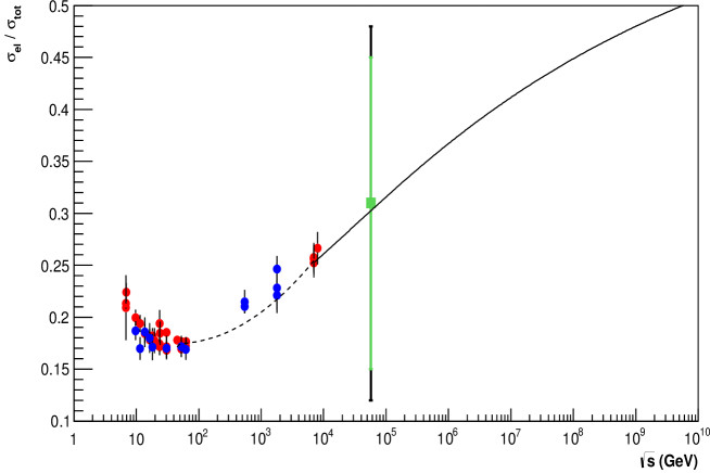
Figure 3: Experimental data from accelerators for the ratio ${\cal R}_{el}=\sigma_{elastic}/\sigma_{total}$ as compiled in [3]. The AUGER datum has been extracted from the ratio $\sigma_{inel}/\sigma_{total}$ at $\sqrt{s}=57$ TeV, as coming from estimates presented in [9]. For this point, the inner bars (green) comprise only statistical and systematic uncertainties combined quadratically and the outer bars (black) incorporate the total uncertainty, with errors from Glauber calculations also summed in quadrature. Inner bars: ${\cal R}_{el}^{\textit{stat+sys}}(57TeV)=0.31^{+0.14}_{-0.16}$, outer bars: ${\cal R}_{el}^{\textit{stat+sys+Glauber}}(57TeV)=0.31^{+0.17}_{-0.19}$.

According to the empirical model presented in this paper, the immediate consequence of this figure is that asymptotia, if defined by the Black Disk (BD) limit ${\cal R}_{el}=1/2$, is still far from having been reached.

2 Geometrical Scaling and the empirical model

In [3] we have assumed Geometrical Scaling (GS) to study the dip shrinkage with growing energy. To do so, we resorted to the ansatz presented in [10]:

$$-t_{dip}(s)=\frac{\tau_{BD}}{2\pi R^{2}(s)[f(s)]^{\alpha}}$$ (8)

where $\tau_{BD}=35.92$ mbGeV² [12] and the function $f(s)$ [11] reflects the evolution of the ratio $\mathcal{R}_{el}$ towards unitarity saturation. The BD model describes the scattering through a purely imaginary one-channel amplitude in b-space, $iR(s)\theta(R(s)-b)$, which is different from zero in a limited region and leads to

$$\sigma_{tot}(s) = 2\pi R^{2}(s),$$ (9)

$$\sigma_{el}(s) = \pi R^{2}(s),$$ (10)

$$\frac{d\sigma_{el}}{dt} = \pi R^{4}\left[\frac{J_{1}(qR)}{qR}\right]^{2}.$$ (11)

The value $\tau_{BD}$ is obtained in the BD model as corresponding to the first zero of the $J_{1}$ function, $x_{0}=\sqrt{-t_{dip}}b_{max}=\sqrt{|t|_{dip}\sigma_{total}/(2\pi)}=\sqrt{\tau_{BD}/2\pi}\approx 3.83$ . In general, the value $\tau_{BD}$ is obtained asymptotically for any one-eikonal model, when the imaginary part of the eikonal function in $b-$space goes to $+\infty$ and the amplitude is just $\theta(b_{max}-b)$ and in momentum space is proportional to a $J_{1}$ function.
We present here a different way to analyze and predict the position of the dip. We start from the consideration that both the experimental data and the empirical model extended to very high energies as seen from Fig. 3, indicate that we are still in a region where there exist two distinct energy scales, one for $\sigma_{total}$ and another for $\sigma_{elastic}$. This is why the variable

$$\tau_{GS}(-t,s)=-t\sigma_{total},$$ (12)

traditionally proposed as proof of geometrical scaling, is not so very precise in predicting the position of the dip at present accelerator energies [10]. Instead, we propose a modified form of GS which is related to the geometric mean of the two still distinct energy scales present at non-asymptotic energies, $\sigma_{total}$ and $\sigma_{elastic}$, namely

$$\tau_{GS}^{mean}(-t,s)=-t\sqrt{\sigma_{elastic}\sigma_{total}}.$$ (13)

Plotting $\tau_{GS}^{mean}(-t_{dip},s)\equiv\tau^{dip}_{GS}$ for energies from ISR to LHC, as we show in Fig. 4, one can compare the behavior with energy of both the traditional and the new variable at $-t=t_{dip}$. We see that the variable $\tau^{dip}_{GS}$ is almost constant within the experimental errors through the entire energy range, from ISR to LHC. The new variable thus appears to be a good predictor for the position of the dip.

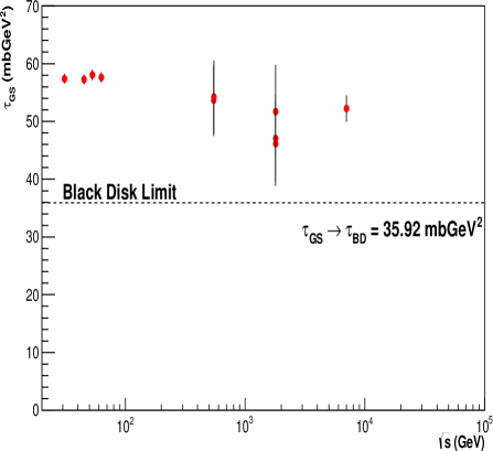
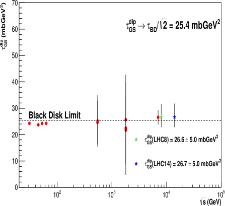
Figure 4: Energy dependence of two possible scaling variables at $-t=t_{dip}$ from ISR to LHC: traditional geometrical scaling at left and the new variable $\tau_{GS}^{mean}$ which uses geometric mean between $\sigma_{total}$ and $\sigma_{elastic}$, at right.

In this figure, the two last points (green and blue stars) are the results from the empirical asymptotic model [3, 4], based on [5], and shown in Eq.  (2). The dashed line in both plots refer to what Refs. [10, 12] define as the Black Disk value.
For the BD model, the two different energy scales, $\sqrt{\sigma_{total}}$ and $\sqrt{\sigma_{elastic}}$ correspond to two radii in $b$-space, $b_{tot}$ and $b_{el}$, which evolve differently as the energy increases. At the BD limit, the two areas will grow together, at the same pace. But until then, one has to live with two scales, namely two areas and thus two radii. In Fig. 5 we show the predictions of model (11) to the differential elastic cross section at $\sqrt{s}=7$ TeV according to the scaling regimes of Eqs. (12) and (13). In this figure the full line shows the predictions of model (11) to the differential elastic cross section at $\sqrt{s}=7$ TeV according to Eqs. (12), and we see that the dip occurs too early, although the optical point is obviously reproduced. The dotted line is a first attempt to incorporate the existence of two radii at non-asymptotic energies, one referring to the elastic cross-section and the other to the total. The dotted curve uses $R^{2}(s)=b_{el}b_{tot}=\sqrt{(\sigma_{elastic}/\pi)(\sigma_{total}/2\pi)}=\sqrt{(\sigma_{elastic}\sigma_{total}/2\pi^{2})}$ in (11) . It gives a good reproduction of the dip position, but the optical point obviously cannot be reproduced.

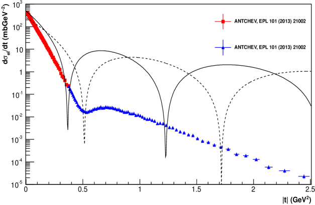
Figure 5: Differential elastic cross section and predictions of the black disk model from Eq. (14-15). The solid curve gives the scaling at the dip according to $\tau_{GS}$ while dashed curve scales with $\tau_{GS}^{mean}$ at $t_{dip}$. Dashed curve is not compatible with the optical point.

More precisely, we have:

• Solid line

  $$\frac{d\sigma_{el}}{dt}=\pi b_{tot}^{4}\left[\frac{J_{1}(qb_{tot})}{qb_{tot}}\right]^{2}\quad;\quad b_{tot}=\sqrt{\frac{\sigma_{tot}}{2\pi}}=6.3\ {GeV}^{-1}$$ (14)

• Dashed line

  $$\frac{d\sigma_{el}}{dt}=\pi R^{4}\left[\frac{J_{1}(qR)}{qR}\right]^{2}\quad;\quad R=\sqrt{b_{el}b_{tot}}=(\sigma_{tot}\sigma_{el}/2\pi^{2})^{1/4}=5.4\ {GeV}^{-1}$$ (15)

The above plot confirms what was shown in Fig. 4, namely that the position of the dip is in fact determined with $1/\sqrt{\sigma_{tot}\sigma_{el}}$ and not with $1/\sigma_{tot}$. Nevertheless, the first scaling gives the proper normalization at the optical point, while the second one does not. Not surprisingly this normalization problem goes away when true asymptotia is achieved, as $\sigma_{el}=\sigma_{tot}/2$ and $R=b_{tot}$, and these curves become essentially one.
However, the obvious fact that the BD model does not reproduce at all the shape of the measured differential elastic cross-section should be noticed: the Fourier transform of the BD amplitude being a step function, quite unlike the shape shown in Fig. 2.

3 New scaling and the differential elastic cross-section data

We have applied the hypothesis of geometric mean scaling to the experimental data for the elastic differential cross-section from ISR to LHC. The result is shown in Fig. 6, with the left hand plot scaling data in the variable $\tau_{GS}$, while the right hand plot shows the behavior in the new variable.

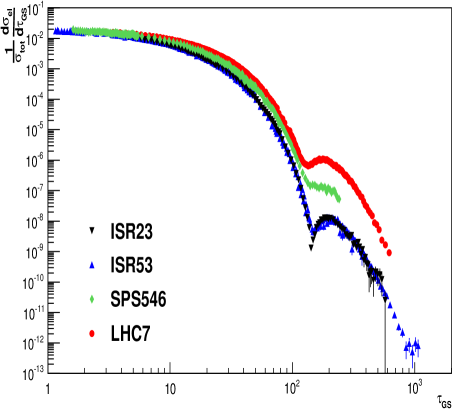
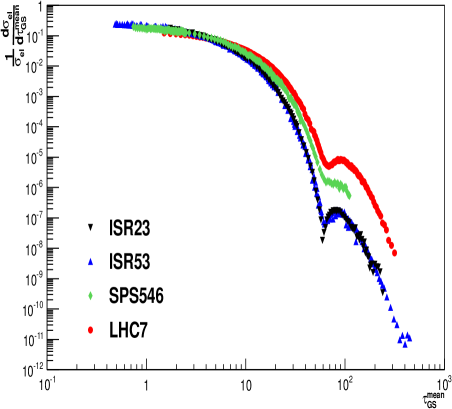
Figure 6: Differential elastic cross section from ISR to LHC as a function of the scaling variable $\tau_{GS}=-t\sigma_{total}(s)$ in the left panel, and $\tau_{GS}^{mean}=-t\sqrt{\sigma_{total}\sigma_{elastic}}$ in the right hand panel.

We see that in both cases there is scaling at ISR energies, but not at higher energy, except that the situation improves for what concerns the position of the dip when scaling is tested in the new variables, $\tau_{GS}^{mean}$.

Similar applications of the scaling hypothesis have been recently tested by Dremin and Nechitailo [13], plotting distributions such as $t^{n}d\sigma_{el}/dt\times t^{m}\sigma_{tot}$ (with $n,m$ reals and $n\neq m$). No genuine scaling was found in the energy region spanning from ISR to LHC.

4 Conclusions

We have presented an analysis of the differential elastic $proton-proton$ cross-section using an empirical model, built with two amplitudes and a relative phase. The model giving a good reproduction of data from ISR to LHC, we have extrapolated it to study the energy behavior of the ratio ${\cal R}_{el}=\sigma_{elastic}/\sigma_{total}$. The fact that we are still very far away from the Black Disk limit ${\cal R}_{el}=1/2$ confirms the already known failure of the variable $\tau_{GS}=|t|\sigma_{total}$ as a valid scaling quantity as the energy increases. In its place, we propose a new scaling variable which takes into account the different energy evolution of $\sigma_{elastic}$ and $\sigma_{total}$.

We find the new variable to be consistent with scaling of the dip position. As for the overall normalization, the differential elastic cross-section confirms scaling of ISR cross-sections, but as the energy increases the curves do not scale.

- [1] \BYAntchev, G. and others \INEurophys.Lett. 101 2013 21002.
- [2] \BYAntchev, G. and others \INPhys. Rev. Lett. 1112013012001.
- [3] \BYFagundes D.A., Grau A., Pacetti S., Pancheri G. \atqueSrivastava, Y.N. \IN Phys. Rev. D88 2013 094019.
- [4] \BYGrau A., Pacetti S., Pancheri G. \atqueSrivastava, Y.N. \IN Phys.Lett. B 714 2012 70.
- [5] \BYPhillips, R. J. N. \atqueBarger, V. D. \INPhys. Lett. B461973412.
- [6] \BYA. Donnachie, A. \atqueLandshoff, P.\INZeit. Phys. C2197955
- [7] \BYA. Donnachie, A. \atqueLandshoff, P.\INPhys. Lett. B7272013500.
- [8] \BYJenkowszky, L. These Proceedings.
- [9] \BYAbreu, P. et al \INPhys.Rev.Lett.1092012062002.
- [10] \BYBautista, I. \atqueDias de Deus, J. \INPhys. Lett. B71820131571.
- [11] \BYFagundes, D.A. \atqueMenon, M.J. \INNucl.Phys. A88020121.
- [12] \BYBrogueira, P. \atquede Deus, J. Dias \INJ.Phys.G392012055006.
- [13] \BYDremin, I.M. \atqueNechitailo, V.A. \INPhys. Lett.B7202013177.