Manipulation of tripartite-to-bipartite entanglement localization under quantum noises and its application to entanglement distribution

Abstract

This paper is to investigate the effects of quantum noises on entanglement localization by taking an example of reducing a three-qubit Greenberger-Horne-Zeilinger (GHZ) state to a two-qubit entangled state. We consider, respectively, two types of quantum decoherence, i.e., amplitude-damping and depolarizing decoherence, and explore the best von Neumann measurements on one of three qubits of the triple GHZ state for making the amount of entanglement of the collapsed bipartite state be as large as possible. The results indicate that different noises have different impacts on entanglement localization, and that the optimal strategy for reducing a three-qubit GHZ state to a two-qubit one via local measurements and classical communications in the amplitude-damping case is different from that in the noise-free case. We also show that the idea of entanglement localization could be utilized to improve the quality of bipartite entanglement distributing through amplitude-damping channels. These findings might shed a new light on entanglement manipulations and transformations.

I Introduction

Establishment of entanglement among distant parties is a prerequisite for implementing lots of remote quantum-information processing tasks 81RMP865 ; 84RMP777 . In situations of practical interest, most of these scenarios involve many parties, and the specific subsets which will carry out quantum communications are not known when the entangled resources are generated and distributed among all of the parties. Particularly, different nodes in a quantum network are usually connected by multipartite entangled states 3NP256 ; 453N1023 , and the two-party quantum communication protocols between any two possible parities are not set in advance. For accomplishing two-party quantum communications, they need to previously establish bipartite entanglement between them via the help of other parties 77PRA022308 . It is hence interesting to search efficient ways to extract entangled states with fewer particles (e.g., two particles) from multiparticle entangled states.

Many theoretical works study, as a method of establishing entanglement between two of many parties who previously share a multipartite entangled state, a reduction the multipartite entangled state to a bipartite entangled state via local measurements assisted by classical communications. Such a paradigm of localizing bipartite entanglement is related to the notions of entanglement-of-assistance EOA ; 3QIC64 , localizable-entanglement 92PRL027901 ; 71PRA042306 , and entanglement-of-collaboration 74PRA052307 . They quantify the maximal average amount of entanglement of two parties that can be extracted from a multipartite entangled state via (local) measurements and different ways of classical communications. From the practical point of view, however, it may be more important to maximize the entanglement between the chosen two parties for specific events, where the desired measurement outcomes of other parties are gotten, as shown in this paper.

The idea of entanglement localization works perfectly for ideally isolated systems. In practice, however, no system can be completely isolated from surroundings 82RMP1155 , and the system will experience decoherence because of the interaction with environment. Multipartite entanglement, which holds much richer quantum correlations than bipartite entanglement, is known to be very fragile to decoherence and to display subtle decay features 100PRL080501 ; 78PRA064301 ; 81PRA064304 ; 45JPB225503 , especially when an entangled multiparticle state is distributed into several distant recipients 453N1023 ; 76RPP096001 . Then the conventional entanglement localization strategies may achieves no longer the optimization. Therefore, it is important to understand and optimize techniques to realize effective entanglement localization in the face of noise and decoherence.

In this paper, we investigate the effects of quantum noises on the tripartite-to-bipartite entanglement localization and the optimal single-particle measurement strategy for reducing a three-qubit Greenberger-Horne-Zeilinger (GHZ) state GHZ to a two-qubit entangled state. We show that the amplitude and depolarizing noises have different impacts on entanglement localization, and that the best von Neumann measurement on one of three qubits of a triple GHZ state for extracting a two-qubit entangled state in the amplitude-damping environment is different from that in the noise-free and depolarizing cases. These results indicate that when considering the amplitude-damping decoherence, the three parties who previously share a three-qubit GHZ state should take different entanglement localization strategy from that in the ideal case, for increasing the amount of entanglement of the final two-qubit entangled state. In addition, we also demonstrate that the idea of entanglement localization could be utilized to improve the quality of bipartite entanglement distribution.

The paper is organized as follows. In section II, we describe the process of entanglement localization from a three-qubit GHZ state to a two-qubit entangled state and give the optimal measurement basis of anyone of the three qubits. In section III, we show how can the idea of entanglement localization boost the quality of bipartite entanglement distribution. Concluding remarks are given in section IV.

II Tripartite-to-bipartite entanglement localization under quantum noises

GHZ states, typical multipartite maximally entangled states, are usually employed for entanglement distribution among different nodes of a quantum network 57PRA822 ; 103PRL020501 , due to the fact that they can be used to implement numerous quantum information protocols 81RMP865 ; 84RMP777 . On the other hand, the characteristics of a GHZ state with many bodies could be usually obtained by straightforwardly generalizing that of tripartite GHZ states 155PLA441 ; 59PRA1829 ; 69PRA052307 ; 8IJQI1301 . In consequence of these facts, we here focus on entanglement localization of tripartite GHZ states. Considering the case that Alice, Bob, and Charlie, staying far away from each other, previously share a three-qubit GHZ state

$$|\psi\rangle^{(123)}=\frac{1}{\sqrt{2}}(|000\rangle+|111\rangle)_{123},$$ (1)

where $\{|0\rangle,|1\rangle\}$ is the computational basis of a qubit. Qubits 1, 2, and 3 are in the labs of Alice, Bob, and Charlie, respectively. Now two of them, e.g., Alice and Bob, want to implement private quantum communication with the existing quantum resource, the GHZ-type entangled state. To this end, they need to first establish bipartite entanglement between them through the assistance of the third party, Charlie. The easiest and robust method is that Charlie performs a local measurement on qubit 3 and broadcasts the outcome, this is so called entanglement localization 92PRL027901 ; 71PRA042306 . Ideally, that is, in the noise-free case, the best measurement that Charlie should adopt is a projective measurement with basis $\left\{|\pm\rangle=(|0\rangle\pm|1\rangle)/\sqrt{2}\right\}$, because Alice and Bob can attain a maximally entangled state, the Bell state $|B_{+}\rangle^{(12)}=(|00\rangle+|11\rangle)_{12}/\sqrt{2}$ or $|B_{-}\rangle^{(12)}=(|00\rangle-|11\rangle)_{12}/\sqrt{2}$, for each possible measurement outcome, $|+\rangle$ or $|-\rangle$. As a matter of fact, the average amount of entanglement between Alice and Bob is one being equivalent to the localizable-entanglement allowed in this case 92PRL027901 ; 71PRA042306 . The procedure of the entanglement localization is schematically sketched in Fig. 1 (a).

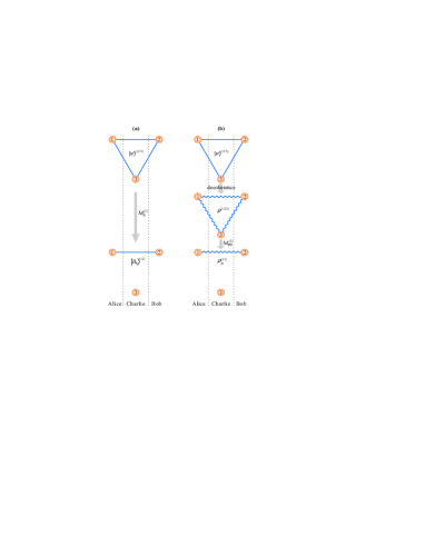
Figure 1: (Color online) Sketch map of entanglement localization for the initial three-qubit GHZ state. Diagram (a) describes the ideal case where the system is isolated perfectly from its surroundings and does not suffer from decoherence; diagram (b) describes the case where each qubit undergoes decoherence before the performance of entanglement localization protocol. The qubits that are linked by straight lines are in a maximally entangled pure state, and that are linked by wave lines are in a mixed state. $M^{(3)}_{\theta\pm}$ ($M^{(3)}_{\pm}$) denotes a von Neumann measurement on qubit 3 with projectors $M^{(3)}_{\theta+}=|+_{\theta}\rangle_{3}\langle+_{\theta}|$ ($M^{(3)}_{+}=|+\rangle_{3}\langle+|$) and $M^{(3)}_{\theta-}=|-_{\theta}\rangle_{3}\langle-_{\theta}|$ ($M^{(3)}_{-}=|-\rangle_{3}\langle-|$), where the measurement basis $\{|+_{\theta}\rangle,|-_{\theta}\rangle\}$ is given in Eq. (II.1).

In practice, qubits 1, 2, and 3 will undergo independently decoherence induced by local noises, and the canonical GHZ state will be converted into a mixed state before we preforming the entanglement localization procedure, as shown in Fig. 1 (b). We first consider the amplitude noise Nielsen in section A, and then discuss other noise models, e.g., depolarizing model Nielsen , in section B.

II.1 Entanglement localization under amplitude-damping decoherence

Amplitude-damping decoherence is suited to many practical qubit systems, including vacuum-single-photon qubit with photon loss, atomic qubit with spontaneous decay, and superconducting qubit with zero-temperature energy relaxation. The action of amplitude noise can be described by two Krauss operators,

$$K_{0}=\left(\begin{array}[]{cc}1&0\\ 0&\sqrt{\overline{d}}\end{array}\right),~{}~{}~{}~{}K_{1}=\left(\begin{array}[]{cc}0&\sqrt{d}\\ 0&0\end{array}\right)$$ (6)

with $0\leqslant d\leqslant 1$ and $\bar{d}=1-d$. $K_{1}$ describes the transition of $|1\rangle$ to $|0\rangle$, while $K_{0}$ describes the evolution of the system without such a transition. Note that $d=0$ denotes the noise-free case and $d=1$ means the interactional time or strength between the system and environment tending to infinity. Therefore, the decoherence strength $d$ is acquiesced in the range $(0,1)$ in the following discussion.

After each qubit interacting with a local amplitude-damping environment, the standard GHZ state in Eq. (1) degenerates to a mixed state

$$\rho^{(123)} = \sum\limits_{l,m,n=0}^{1}K_{l}\otimes K_{m}\otimes K_{n}|\psi\rangle^{(123)}\langle\psi|K_{l}^{+}\otimes K_{m}^{+}\otimes K_{n}^{+}$$ (7)

$$= \frac{1}{2}(1+d_{1}d_{2}d_{3})|000\rangle\langle 000|+\frac{1}{2}\bar{d}_{1}\bar{d}_{2}\bar{d}_{3}|111\rangle\langle 111|$$

$$+\frac{1}{2}\sqrt{\bar{d}_{1}\bar{d}_{2}\bar{d}_{3}}|000\rangle\langle 111|+\frac{1}{2}\sqrt{\bar{d}_{1}\bar{d}_{2}\bar{d}_{3}}|111\rangle\langle 000|$$

$$+\frac{1}{2}d_{1}d_{2}\bar{d}_{3}|001\rangle\langle 001|+\frac{1}{2}d_{1}\bar{d}_{2}d_{3}|010\rangle\langle 010|$$

$$+\frac{1}{2}\bar{d}_{1}d_{2}d_{3}|100\rangle\langle 100|+\frac{1}{2}d_{1}\bar{d}_{2}\bar{d}_{3}|011\rangle\langle 011|$$

$$+\frac{1}{2}\bar{d}_{1}d_{2}\bar{d}_{3}|101\rangle\langle 101|+\frac{1}{2}\bar{d}_{1}\bar{d}_{2}d_{3}|110\rangle\langle 110|,$$

where $d_{1}$, $d_{2}$, and $d_{3}$ denote the decoherence strengths of qubits 1, 2, and 3, respectively. For helping Alice and Bob to establish a two-qubit entangled state with as much entanglement as possible, Charlie needs to make a suitable local measurement on qubit 3 and informs them of the outcome. We here only pay attention to the von Neumann measurement. The general single-qubit projective measurement basis can be described by

$$|+_{\theta}\rangle = \cos\frac{\theta}{2}|0\rangle+\sin\frac{\theta}{2}e^{i\varphi}|1\rangle,$$

$$|-_{\theta}\rangle = \sin\frac{\theta}{2}e^{-i\varphi}|0\rangle-\cos\frac{\theta}{2}|1\rangle,$$ (8)

where $\theta\in[0,\pi]$ and $\varphi\in[0,2\pi]$. When $\theta=\pi/2$ and $\varphi=0$, $|\pm_{\theta}\rangle$ reduce to $|\pm\rangle$. The probability of getting the outcome $|+_{\theta}\rangle_{3}$ is given by

$$P_{+}(d,\theta) = \mathrm{Tr}\left[|+_{\theta}\rangle_{3}\langle+_{\theta}|\rho^{(123)}\right]$$ (9)

$$= \frac{1}{2}+\frac{d_{3}}{2}\cos\theta.$$

The occurrence of this event will lead to the fact that qubits 1 and 2 are projected in the state

$$\rho^{(12)}_{+} = \frac{1}{P_{+}}\mathrm{Tr}_{3}\left[|+\rangle_{3}\langle+|\rho^{(123)}\right]$$ (10)

$$= \frac{1}{P_{+}}\left(\gamma_{+}|00\rangle\langle 00|+\kappa_{+}|01\rangle\langle 01|+\tau_{+}|10\rangle\langle 10|\right.$$

$$\left.+\eta_{+}|11\rangle\langle 11|+\xi|00\rangle\langle 11|+\xi^{*}|11\rangle\langle 00|\right),$$

where

$$\gamma_{+} = \frac{1}{2}(1+d_{1}d_{2}d_{3})\cos^{2}\frac{\theta}{2}+\frac{1}{2}d_{1}d_{2}\bar{d}_{3}\sin^{2}\frac{\theta}{2},$$

$$\kappa_{+} = \frac{1}{2}d_{1}\bar{d}_{2}d_{3}\cos^{2}\frac{\theta}{2}+\frac{1}{2}d_{1}\bar{d}_{2}\bar{d}_{3}\sin^{2}\frac{\theta}{2},$$

$$\tau_{+} = \frac{1}{2}\bar{d}_{1}d_{2}d_{3}\cos^{2}\frac{\theta}{2}+\frac{1}{2}\bar{d}_{1}d_{2}\bar{d}_{3}\sin^{2}\frac{\theta}{2},$$

$$\eta_{+} = \frac{1}{2}\bar{d}_{1}\bar{d}_{2}d_{3}\cos^{2}\frac{\theta}{2}+\frac{1}{2}\bar{d}_{1}\bar{d}_{2}\bar{d}_{3}\sin^{2}\frac{\theta}{2},$$

$$\xi = \frac{1}{2}\sqrt{\bar{d}_{1}\bar{d}_{2}\bar{d}_{3}}\sin\frac{\theta}{2}\cos\frac{\theta}{2}e^{i\varphi}.$$ (11)

If the measurement outcome on qubit 3 is $|-_{\theta}\rangle_{3}$, which happens with probability

$$P_{-}(d,\theta) = \mathrm{Tr}\left[|-\rangle_{3}\langle-|\rho^{(123)}\right]=1-P_{+}(d,\theta)$$ (12)

$$= \frac{1}{2}-\frac{d_{3}}{2}\cos\theta,$$

qubits 1 and 2 will be projected in the state

$$\rho^{(12)}_{-} = \frac{1}{P_{-}}\mathrm{Tr}_{3}\left[|-\rangle_{3}\langle-|\rho^{(123)}\right]$$ (13)

$$= \frac{1}{P_{-}}\left(\gamma_{-}|00\rangle\langle 00|+\kappa_{-}|01\rangle\langle 01|+\tau_{-}|10\rangle\langle 10|\right.$$

$$\left.+\eta_{-}|11\rangle\langle 11|-\xi|00\rangle\langle 11|-\xi^{*}|11\rangle\langle 00|\right),$$

where

$$\gamma_{-} = \frac{1}{2}(1+d_{1}d_{2}d_{3})\sin^{2}\frac{\theta}{2}+\frac{1}{2}d_{1}d_{2}\bar{d}_{3}\cos^{2}\frac{\theta}{2},$$

$$\kappa_{-} = \frac{1}{2}d_{1}\bar{d}_{2}d_{3}\sin^{2}\frac{\theta}{2}+\frac{1}{2}d_{1}\bar{d}_{2}\bar{d}_{3}\cos^{2}\frac{\theta}{2},$$

$$\tau_{-} = \frac{1}{2}\bar{d}_{1}d_{2}d_{3}\sin^{2}\frac{\theta}{2}+\frac{1}{2}\bar{d}_{1}d_{2}\bar{d}_{3}\cos^{2}\frac{\theta}{2},$$

$$\eta_{-} = \frac{1}{2}\bar{d}_{1}\bar{d}_{2}d_{3}\sin^{2}\frac{\theta}{2}+\frac{1}{2}\bar{d}_{1}\bar{d}_{2}\bar{d}_{3}\cos^{2}\frac{\theta}{2}.$$ (14)

Next, we use two measures, negativity 58PRL883 ; 65PRA032314 and fully entangled fraction (FEF) 54PRA3824 ; 60PRA1888 , to quantify the entanglement of $\rho_{+}^{(12)}$ and $\rho_{-}^{(12)}$, respectively, and analyze their features. Negativity has been considered as a dependable measure of entanglement for bipartite entangled states 58PRL883 ; 65PRA032314 . FEF, which expresses the purity of a bipartite mixed state, plays a central role in quantum teleportation and entanglement distillation 54PRA3824 ; 60PRA1888 ; 76PRL722 ; 78PRL574 , and may behave differently from negativity as shown later.

II.1.1 Negativity of the collapsed state of qubits 1 and 2

Following Ref. 58PRL883 , we use the following definition of negativity:

$$N(\rho)=\max\left\{0,-2\lambda_{\mathrm{min}}(\rho)\right\},$$ (15)

with $\lambda_{\mathrm{min}}$ the minimal eigenvalue of the partial transpose of $\rho$ denoted as $\rho^{T}$. After straightforward calculations we obtain the negativity of $\rho_{+}^{(12)}$ and $\rho_{-}^{(12)}$ as

$$N_{+}(\rho_{+})=\max\left\{0,-2\mu_{+}\right\},$$ (16)

$$N_{-}(\rho_{-})=\max\left\{0,-2\mu_{-}\right\},$$ (17)

where $\mu_{+}$ and $\mu_{-}$ are, respectively, the minimal eigenvalues of $\rho_{+}$ and $\rho_{-}$, given by

$$\mu_{+}=\frac{1}{2P_{+}}\left(\kappa_{+}+\tau_{+}-\sqrt{(\kappa_{+}-\tau_{+})^{2}+4|\xi|^{2}}\right),$$ (18)

$$\mu_{-}=\frac{1}{2P_{-}}\left(\kappa_{-}+\tau_{-}-\sqrt{(\kappa_{-}-\tau_{-})^{2}+4|\xi|^{2}}\right).$$ (19)

For clarity, we give a detailed analysis on $N_{+}$ and $N_{-}$ for the case $d_{1}=d_{2}=d_{3}=d$ (which is not a necessary assumption but only simplifies the degree of algebraic complexity). In this case, $\mu_{+}$ and $\mu_{-}$ reduce, respectively, to

$$\mu^{s}_{+}=\frac{\bar{d}}{2P_{+}}\left(d^{2}\cos^{2}\frac{\theta}{2}+d\bar{d}\sin^{2}\frac{\theta}{2}-\sqrt{\bar{d}~{}}\sin\frac{\theta}{2}\cos\frac{\theta}{2}\right),$$ (20)

$$\mu^{s}_{-}=\frac{\bar{d}}{2P_{-}}\left(d^{2}\sin^{2}\frac{\theta}{2}+d\bar{d}\cos^{2}\frac{\theta}{2}-\sqrt{\bar{d}~{}}\sin\frac{\theta}{2}\cos\frac{\theta}{2}\right).$$ (21)

The clear dependence of $N_{+}$ and $N_{-}$ on $d$ and $\theta$ is plotted in Fig. 2.

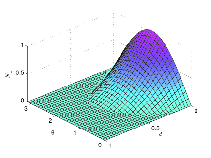
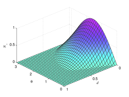
Figure 2: (Color online) The function graph of $N_{+}$ and $N_{-}$ with respect to $d$ and $\theta$.

It can be seen from Fig. 2 that when $d$ increases to a threshold, being away from one, for a given $\theta$, both $N_{+}$ and $N_{-}$ decrease to zero. This indicates that the entanglement vanishes in a finite time, which is referred to as entanglement sudden death 316S579 ; 93PRL140404 ; 99PRL180504 ; 99PRL160502 ; 76PRA062322 . More interesting and important information that can be obtained from Fig. 2 is as follows. If $d=0$ (corresponding to the absence of noise), both of $N_{+}$ and $N_{-}$ attain their maximal values at $\theta=\pi/2$, meaning that $\{|\pm\rangle_{3}\}$ is the optimal measurement basis. This result is in accordance with the discussion before. For $d>0$, however, both $N_{+}$ and $N_{-}$ are asymmetric with respect to $\theta=\pi/2$ in the region that $d$ is less than the threshold defined above. This feature implies that $N_{+}$ and $N_{-}$ reach their maximums at the points that deviate from $\theta=\pi/2$, respectively. Such phenomena can be observed clearly in Fig. 3 which gives the bivariate functions $\Delta N_{+}(d,\theta)=N_{+}(d,\theta)-N_{+}(d,\theta=\pi/2)$ and $\Delta N_{-}(d,\theta)=N_{-}(d,\theta)-N_{-}(d,\theta=\pi/2)$ with independent variables $\theta$ and $d$. We can see that there exist different regimes of $\theta$ in which $\Delta N_{+}$ and $\Delta N_{-}$ are larger than zero, respectively; that is, $N_{+}(d,\theta\neq\pi/2)$ and $N_{-}(d,\theta\neq\pi/2)$ are indeed larger than $N_{+}(d,\pi/2)$ and $N_{-}(d,\pi/2)$, respectively. These results indicate that Charlie can enhance probabilistically the entanglement distributed between Alice and Bob by selecting an appropriate measurement basis $\{|+_{\theta\neq\pi/2}\rangle,|-_{\theta\neq\pi/2}\rangle\}$ instead of $\{|+\rangle,|-\rangle\}$.

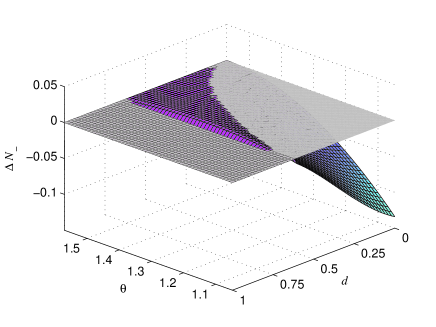
Figure 3: (Color online) The dependence of $\Delta N_{+}$ and $\Delta N_{-}$ on $d$ and $\theta$, where $\theta$ ranges from $\pi/2$ to $2\pi/3$ in the upper graph and from $\pi/3$ to $\pi/2$ in the lower graph.

The average amount of entanglement between qubits 1 and 2 for two possible measurement outcomes $|+_{\theta}\rangle$ and $|-_{\theta}\rangle$ is given by

$$N_{\mathrm{ave}}(d,\theta)=P_{+}N_{+}+P_{-}N_{-}.$$ (22)

It can be easily verified that when $d$ is smaller than a threshold, the maximal value of $N_{\mathrm{ave}}(d,\theta)$ is $N_{\mathrm{ave}}(d,\pi/2)$ for a given $d$. When $d$ goes beyond the threshold, however, $N_{\mathrm{ave}}(d,\theta)$ can attain its maximum at two different values of $\theta$, situating symmetrically on the two sides of $\theta=\pi/2$, provided that $N_{\mathrm{ave}}(d,\theta)$ is not always equal to zero, as shown in Fig. 4; this fact means that $\{|\pm\rangle\}$ is no longer the optimal measurement basis of qubit 3. Figure 4 also indicates that the existing time of the entanglement of the state $\rho_{+}$ or $\rho_{-}$ can be protracted by taking an appropriate measurement basis $\{|+_{\theta\neq\pi/2}\rangle,|-_{\theta\neq\pi/2}\rangle\}$ instead of $\{|+\rangle,|-\rangle\}$.

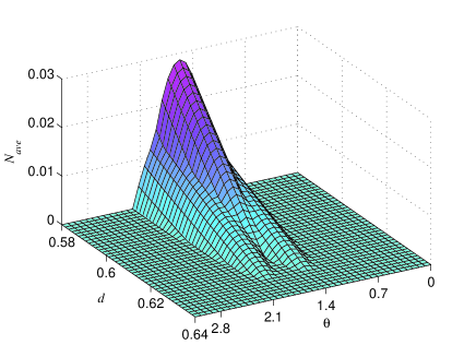
Figure 4: (Color online) $N_{\mathrm{ave}}$ versus $d$ and $\theta$. The figure only plots the region of $0.58\leqslant d\leqslant 0.64$.

In the discussion above, we supposed that everyone of three qubits suffer decoherence. The obtained result is naturally applicable to special cases. That is, when only one or two qubits sustain decoherence, the optimal measurement basis of qubit 3 is also not $\{|+\rangle,|-\rangle\}$. Let us take an example of $d_{3}=0$ and $d_{1}=d_{2}=d$. Then $N_{+}$ and $N_{-}$ in Eqs. (16) and (17) reduce, respectively, to

$$N_{+}=\max\left\{0,~{}2\bar{d}\sin\frac{\theta}{2}\left(\cos\frac{\theta}{2}-d\sin\frac{\theta}{2}\right)\right\},$$ (23)

$$N_{-}=\max\left\{0,~{}2\bar{d}\cos\frac{\theta}{2}\left(\sin\frac{\theta}{2}-d\cos\frac{\theta}{2}\right)\right\},$$ (24)

Evidently, the points of maximum of both $N_{+}$ and $N_{-}$ are not at $\theta=\pi/2$. That is to say, the best measurement basis of qubit 3 is not $\{|+\rangle,|-\rangle\}$ in the aforementioned entanglement localization protocol.

II.1.2 FEF of the collapsed state of qubits 1 and 2

FEF of a state $\rho$ is defined as the maximum overlap of $\rho$ with a maximally entangled state 54PRA3824 ; 60PRA1888 , that is,

$$F(\rho)=\max\limits_{|\phi\rangle}\langle\phi|\rho|\phi\rangle,$$ (25)

where the maximization is taken over all maximally entangled states $|\phi\rangle$. For two-qubit systems $F(\rho)$ can be analytically expressed as 62PRA012311

$$F(\rho)=\frac{1}{4}\left\{1+\mu_{1}+\mu_{2}-\mathrm{sgn}[\det(\tilde{R})]\mu_{3}\right\},$$ (26)

where $\{\mu_{i}\}$ are the decreasingly ordered singular values of the $3\times 3$ real matrix $\tilde{R}=\left[\mathrm{tr}(\rho\sigma_{i}\otimes\sigma_{j})\right]_{3\times 3}$ with $\{\sigma_{i},i=1,2,3\}$ the Pauli matrices and $\mathrm{sgn}[\det(\tilde{R})]$ is the sign of the determinant of $\tilde{R}$.

The FEF of the states $\rho_{+}$ and $\rho_{-}$ in Eq. (10) and Eq. (13) can be calculated to be

$$F_{+}(\rho_{+}) = \frac{1}{4}+\frac{\left(4|\xi|+\gamma_{+}+\eta_{+}-\kappa_{+}-\tau_{+}\right)}{4P_{+}},$$ (27)

$$F_{-}(\rho_{-}) = \frac{1}{4}+\frac{\left(4|\xi|+\gamma_{-}+\eta_{-}-\kappa_{-}-\tau_{-}\right)}{4P_{-}}.$$ (28)

As before, we still discuss the case $d_{1}=d_{2}=d_{3}=d$. Then $F_{+}(\rho_{+})$ and $F_{-}(\rho_{-})$ reduce, respectively, to

$$F_{+}(d,\theta) = \frac{1}{2}-\mu^{s}_{+},$$ (29)

$$F_{-}(d,\theta) = \frac{1}{2}-\mu^{s}_{-}.$$ (30)

Then the FEF $F_{+}$ and $F_{-}$ have the similar behaviors to the negativity $N_{+}$ and $N_{-}$, respectively. That is, $F_{+}$ and $F_{-}$ reach their maximal values at $\theta\neq\pi/2$. As a matter of fact, $F_{+}$ ($F_{-}$) and $N_{+}$ ($N_{-}$) have the same extremal point, and there exist the same scale of $d$ in which $F_{+}(d,\theta)$ [$F_{-}(d,\theta)$] and $N_{+}(d,\theta)$ [$N_{-}(d,\theta)$] are larger than $F_{+}(d,\theta=\pi/2)$ [$F_{-}(d,\theta=\pi/2)$] and $N_{+}(d,\theta=\pi/2)$ [$N_{-}(d,\theta=\pi/2)$], respectively. Thus Charlie can also increase the FEF of the state shared by Alice and Bob by adopting a suitable measurement basis $\{|+_{\theta\neq\pi/2}\rangle,|-_{\theta\neq\pi/2}\rangle\}$ instead of $\{|+\rangle,|-\rangle\}$.

The mean value of $F_{+}$ and $F_{-}$ can be calculated as

$$F_{\mathrm{ave}} = P_{+}F_{+}+P_{-}F_{-}$$

$$= \frac{3}{8}+\sqrt{\bar{d}_{1}\bar{d}_{2}\bar{d}_{3}}\sin\frac{\theta}{2}\cos\frac{\theta}{2}+\frac{1}{8}(2d_{1}-1)(2d_{2}-1).$$

For $d_{1}=d_{2}=d_{3}=d$, $F_{\mathrm{ave}}$ reduces to

$$F_{\mathrm{ave}}(d,\theta)=\frac{3}{8}+\bar{d}\sqrt{\bar{d}~{}}\sin\frac{\theta}{2}\cos\frac{\theta}{2}+\frac{1}{8}(2d-1)^{2}.$$ (32)

Obviously, the maximal value of $F_{\mathrm{ave}}(d,\theta)$ is $F_{\mathrm{ave}}^{\mathrm{max}}(d)=F_{\mathrm{ave}}(d,\theta=\pi/2)$ which is independent of the parameter $\theta$. This result indicates that $F_{\mathrm{ave}}$ has different behavior to $N_{\mathrm{ave}}(d,\theta)$ which reaches the maximal value at $\theta\neq\pi/2$ when $d$ oversteps a critical value (see Fig. 4).

In view of practice, however, what we are interested in is to maximize $F_{+}$ or $F_{-}$, due to the fact that the larger the FEF is, the higher teleportation fidelity and entanglement purification efficiency can be achieved 54PRA3824 ; 60PRA1888 ; 76PRL722 ; 78PRL574 . Moreover, we notice that if and only if the FEF of a two-qubit state $\rho$ is larger than 1/2, quantum teleportation can exhibit its superiority over state estimation based on classical strategies and entanglement purification can be carried out effectively using the resource state $\rho$ 54PRA3824 ; 60PRA1888 ; 76PRL722 ; 78PRL574 . We observe that $F_{\mathrm{ave}}(d,\theta)\leqslant 1/2$ does not mean $F_{+}(d,\theta)$ and $F_{-}(d,\theta)$ are simultaneously less than $1/2$. In deed, when $d\geqslant\left(\sqrt{5}-1\right)/2$, $F_{\mathrm{ave}}^{\mathrm{max}}\leqslant 1/2$ [obtained from Eq. (32)], indicating that the resource state is useless for quantum teleportation and entanglement distillation, while $F_{+}(d,\theta>\pi/2)$ or $F_{-}(d,\theta<\pi/2)$ can overtop $1/2$ as displayed in Fig. 5. Thus we could safely conclude that when we take the measurement strategy that maximizes $F_{\mathrm{ave}}$, both $\rho_{+}$ and $\rho_{-}$ may be useless for quantum teleportation and entanglement distillation; in contrast, if we select an appropriate measurement basis $\{|\pm_{\theta\neq\pi/2}\rangle\}$ rather than $\{|\pm\rangle\}$ such that $F_{\mathrm{ave}}<F_{\mathrm{ave}}^{\mathrm{max}}$, Alice and Bob can implement effective teleportation and entanglement distillation with a nonzero probability. In other words, $\{|\pm\rangle_{3}\}$ is not the best measurement basis for optimizing the robustness of the entangled state of qubits 1 and 2.

It has been mentioned before that maximizing the average amount of entanglement between two particles of a multiparticle state by performing local measurements on the other particles is defined as localizable-entanglement 92PRL027901 ; 71PRA042306 . The conclusions presented above imply that localizable-entanglement is not suitable to be described by the entanglement measure of FEF from the practical point of view.

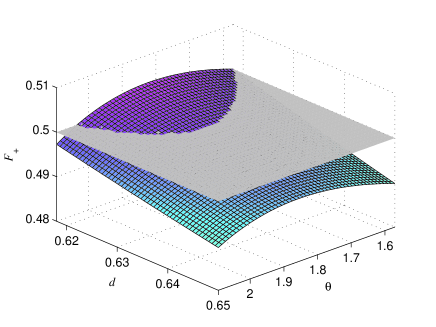
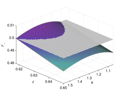
Figure 5: (Color online) $F_{+}$ and $F_{-}$ versus $d$ and $\theta$, where $d$ is in the range $[(\sqrt{5}-1)/2,0.65]$ and $\theta$ is in the range $[\pi/2,2\pi/3]$ for the upper diagram and $[\pi/3,\pi/2]$ for the lower diagram.

Although FEF may be not monotonic in the regime of small values under trace-preserving local operations and classical communication (TPLOCC) for mixed states 62PRA012311 ; 65PRA022302 ; 90PRL097901 ; 86PRA020304 , the aforesaid conclusions are reliable as explained below. The expressions of FEF in Eq. (29) and Eq. (30) can be rewritten as

$$F_{+}(d,\theta)=\left\{\begin{array}[]{ll}\frac{1}{2}(1-2\mu^{s}_{+})&~{}~{}~{}\mathrm{for}~{}~{}N_{+}=0~{}~{}(\mu^{s}_{+}\geqslant 0),\\ \\ \frac{1}{2}(1+N_{+})&~{}~{}~{}\mathrm{for}~{}~{}N_{+}>0~{}~{}(\mu^{s}_{+}<0),\end{array}\right.$$ (36)

$$F_{-}(d,\theta)=\left\{\begin{array}[]{ll}\frac{1}{2}(1-2\mu^{s}_{-})&~{}~{}~{}\mathrm{for}~{}~{}N_{-}=0~{}~{}(\mu^{s}_{-}\geqslant 0),\\ \\ \frac{1}{2}(1+N_{-})&~{}~{}~{}\mathrm{for}~{}~{}N_{-}>0~{}~{}(\mu^{s}_{-}<0).\end{array}\right.$$ (40)

It is well known that TPLOCC cannot create entanglement and thus cannot increase $N_{+}$ or $N_{-}$. Then, TPLOCC cannot increase $F_{+}$ or $F_{-}$ in the present case because of the relationships given in Eqs. (29) and (30), which is in accordance with the result of Ref. 66PRA022307 . In fact, both states $\rho_{+}$ and $\rho_{-}$ do not belong to the class of states presented in Refs. 62PRA012311 ; 65PRA022302 whose FEF may be slightly raised by TPLOCC operations. The same argument could be obtained for the results in the following context. Thus we will not consider the local manipulations on qubits 1 and 2 and the classical communications between Alice and Bob themselves later.

II.2 Entanglement localization under depolarizing decoherence

In the former subsection, we have shown that the optimal strategy for extracting a two-qubit entangled state from a three-qubit GHZ state via local measurements in the amplitude-damping case is different from that in the noise-free case. Particularly, in the ideal case, the best measurement basis of qubit 3 for reducing the three-qubit GHZ state $|\psi\rangle^{(123)}$ to a two-qubit entangled state $\rho^{(12)}$ is $\{|+\rangle_{3},|-\rangle_{3}\}$; while considering the amplitude-damping decoherence of part or all of these qubits, the best measurement basis of qubit 3 is no longer $\{|+\rangle_{3},|-\rangle_{3}\}$. This phenomenon does not necessarily occur under other noise models. We here take an example of depolarizing model.

The single-qubit depolarizing channel is described as

$$\mathcal{E}(\rho)=\sum\limits_{i=0}^{3}p_{i}\sigma_{i}\rho\sigma_{i}$$ (41)

where $\rho$ is the input state of the qubit, $p_{0}=1-d$ and $p_{i}=d/3$ ($i=1,2,3$) with $d$ being the degree of decoherence ($0\leq d\leq 1$), $\sigma_{0}$ is the identity operator, and $\{\sigma_{i}\}$ ($i=1,2,3$) are the Pauli operators $\sigma_{x}$, $\sigma_{y}$, $\sigma_{z}$, respectively.

For the initial three-qubit GHZ state $|\psi\rangle^{(123)}$ in Eq. (1), the depolarizing operation on each qubit will result in it becoming

$$\rho\prime^{(123)}=\sum\limits_{i,j,k=0}^{3}p_{i}p_{j}p_{k}\sigma_{i}\otimes\sigma_{j}\otimes\sigma_{k}|\psi\rangle\langle\psi|\sigma_{i}\otimes\sigma_{j}\otimes\sigma_{k}.$$ (42)

Without loss of generality, we consider that the degree of decoherence of every qubit is not zero. For simplicity, we suppose the qubits have the same degree of decoherence $d$. After the aforementioned entanglement localization process, the negativity of the final state of qubits 1 and 2 is

$$\mathcal{N}=\max\left\{0,-2\lambda\right\},$$ (43)

where $\lambda=2(3-2d)d/9-|3-4d|^{3}\sin\theta/54$ for both the measurement outcomes $|+_{\theta}\rangle_{3}$ and $|-_{\theta}\rangle_{3}$ of qubit 3. In order to guarantee $\mathcal{N}>0$, the condition

$$\sin\theta>\frac{12(3-2d)d}{|3-4d|^{3}}$$ (44)

should be satisfied. Then the point of maximum of $\mathcal{N}$ is at $\theta=\pi/2$ for any $d$. Moreover, the condition of Eq. (44) in the case $\theta=\pi/2$ can be satisfied more easily than in the case $\theta\neq\pi/2$. Thus, the optimal measurement basis of qubit 3 is $\{|+_{\theta=\pi/2}\rangle=|+\rangle,|-_{\theta=\pi/2}\rangle=|-\rangle\}$. Similarly, using the entanglement measure of FEF, the same conclusion can be obtained. In a word, the optimal strategy for reducing a three-qubit GHZ state to a two-qubit entangled state via local measurements in the depolarizing case is the same as that in the noise-free case.

The results above indicate that depolarizing and amplitude-damping noises have different effects on entanglement localization. It tells us that in different environments, we should take different strategies for optimizing the entanglement localization schemes.

III Bipartite entanglement distribution assisted by three-particle entangled states

Inspired by the afore-cited phenomena in section II, we find that multiparticle entangled states could help to improve the quality of entanglement distribution between two distant parties in noisy environments, as demonstrated in this section.

A routine way of bipartite entanglement distributing between two distant parties, Alice and Bob, is to generate a two-qubit entangled state, e.g., a Bell state, in a server, say Charlie, and then physically send the two qubits to the labs of Alice and Bob, respectively. We here propose another way that first preparing a three-qubit entangled state, GHZ state, in Charlie’s site and then send any two qubits, e.g., qubits 1 and 2, to Alice and Bob, one person one qubit, followed by the entanglement localization procedure introduced in the former section. In the noise-free case, the two methods will achieve the same result in terms of the shared entanglement between Alice and Bob. However, when considering the unavoidable effect of noises on the systems during their transmission, the latter scheme could boost probabilistically the amount of entanglement of the two-qubit state shared by Alice and Bob, as shown below. For clarity, the first method will be called direct distribution scheme, DDS for short, and the second one will be referred to as ancilla-assisted distribution scheme abbreviated to ADS. The schematic diagrams of both DDS and ADS are sketched in Fig. 6. The detailed descriptions on the DDS and ADS are given in sections A and B, respectively.

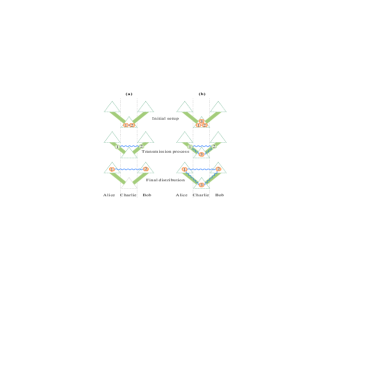
Figure 6: (Color online) Two schemes for distributing bipartite entanglement. (a) Direct distribution scheme (DDS). (b) Ancilla-assisted distribution scheme (ADS), where the process of entanglement localization is not shown in the diagram and the detailed description on it is given in the context (see also Fig. 1). The green bars denote the quantum channels with which Charlie sends particles 1 and 2 to Alice and Bob, respectively. Linking the qubits by beelines denote that these qubits are in a maximally entangled pure state, while linking the qubits by wave lines denote these qubits being in a mixed state.

III.1 DDS for distributing bipartite entanglement via noisy quantum channels

In order to display the advantages of ADS later, we first recapitulate the results of DDS for providing a sharp contrast. Suppose that qubits 1 and 2 are initially prepared in a Bell state

$$|\phi\rangle_{12}=\frac{1}{\sqrt{2}}(|00\rangle+|11\rangle)_{12}.$$ (45)

After the two qubits independently interacting with their environments via amplitude-damping channels, the Bell state evolves into a mixed state

$$\varrho_{12} = \sum\limits_{m,n=0}^{1}K_{m}\otimes K_{n}|\phi\rangle_{12}\langle\phi|K_{m}^{+}\otimes K_{n}^{+}$$ (46)

$$= \frac{1}{2}(1+d_{1}d_{2})|00\rangle\langle 00\rangle+\frac{1}{2}\bar{d}_{1}\bar{d}_{2}|11\rangle\langle 11|$$

$$+\frac{1}{2}\sqrt{\bar{d}_{1}\bar{d}_{2}}|00\rangle\langle 11|+\frac{1}{2}\sqrt{\bar{d}_{1}\bar{d}_{2}}|11\rangle\langle 00|$$

$$+\frac{1}{2}d_{1}\bar{d}_{2}|01\rangle\langle 01|+\frac{1}{2}\bar{d}_{1}d_{2}|10\rangle\langle 10|.$$

The negativity and FEF of $\varrho$ can be calculated, respectively, to be

$$N(\varrho) = \max\left\{0,-2\lambda_{\mathrm{min}}(\varrho)\right\},$$ (47)

$$\lambda_{\mathrm{min}} = \frac{1}{4}\left(d_{1}\bar{d}_{2}+\bar{d}_{1}d_{2}\right)-\frac{1}{4}\sqrt{(d_{1}-d_{2})^{2}+4\bar{d}_{1}\bar{d}_{2}},$$

$$F(\varrho) = \frac{1}{4}\left(2+2\sqrt{\bar{d}_{1}\bar{d}_{2}}+2d_{1}d_{2}-d_{1}-d_{2}\right).$$ (48)

We assume $d_{1}=d_{2}=d$, that is, the decoherence strengths of both qubits are the same. This is not a necessary assumption but only simplifies the degree of algebraic complexity, which makes no difference to the final conclusion. Then $N(\varrho)$ and $F(\varrho)$ reduce to

$$N^{\prime}(\varrho) = (1-d)^{2},$$ (49)

$$F^{\prime}(\varrho) = \frac{1}{2}\left(1+N^{\prime}\right).$$ (50)

III.2 ADS for distributing bipartite entanglement via noisy quantum channels

Some results in Sec. II can be transplanted to this section for simplifying the discussion on the ADS of bipartite entanglement distribution. It is observed from Sec. II that the negativity and FEF of the states $\rho_{+}$ and $\rho_{-}$ are symmetric about $\theta=\pi/2$. Thus we here only discuss the entanglement properties of $\rho_{+}$, and the counterparts for $\rho_{-}$ can be directly obtained using the symmetry.

Following Eq. (16) and Eq. (27), when $d_{1}=d_{2}=d$, $N_{+}(\rho_{+})$ and $F_{+}(\rho_{+})$ reduce to

$$N^{\prime}_{+}(\rho_{+}) = \max\left\{0,\frac{2}{P_{+}}\left(|\xi^{\prime}|-\kappa^{\prime}_{+}\right)\right\},$$ (51)

$$F^{\prime}_{+}(\rho_{+}) = \left\{\begin{array}[]{ll}\frac{1}{2}+\frac{1}{P_{+}}\left(\kappa^{\prime}_{+}-|\xi^{\prime}|\right)&~{}~{}\mathrm{for}~{}N_{+}=0,\\ \\ \frac{1}{2}(1+N^{\prime}_{+})&~{}~{}\mathrm{for}~{}N_{+}>0,\end{array}\right.$$ (55)

where

$$\kappa^{\prime}_{+} = \frac{d\bar{d}}{2}\left(d_{3}\cos^{2}\frac{\theta}{2}+\bar{d}_{3}\sin^{2}\frac{\theta}{2}\right),$$

$$|\xi^{\prime}| = \frac{\bar{d}}{2}\sqrt{\bar{d}_{3}}\sin\frac{\theta}{2}\cos\frac{\theta}{2}.$$ (56)

We now make a comparison between the aforementioned two strategies, DDS and ADS, by analyzing the differences of the negativity and FEF of the state $\rho_{+}$ with that of the state $\varrho$, which are given by

$$\delta N = N^{\prime}_{+}(\rho_{+})-N^{\prime}(\varrho),$$ (57)

$$\delta F = F^{\prime}_{+}(\rho_{+})-F^{\prime}(\varrho).$$ (58)

What we are interested in is whether $\delta N$ and $\delta F$ could be larger than zero. This expectation is possible if and only if $N^{\prime}_{+}(\rho_{+})>0$ and $F^{\prime}_{+}(\rho_{+})>1/2$. According to Eqs. (49)-(55), it can be acquired that $\delta N$ and $\delta F$ have the same behavior in the regime of $N^{\prime}_{+}(\rho_{+})>0$ and $F^{\prime}_{+}(\rho_{+})>1/2$. Thus we only need to analyze the characteristics of $\delta N$, with which the features of $\delta F$ can also be derived straightforwardly.

To exhibit ADS’s superiority clearly, we first assume $d_{3}=0$, meaning that qubit 3 is well isolated from the noisy environment in Charlie’s lab. In this case, the dependence of $\delta N$ on $d$ and $\theta$ is given in Fig. 7 with $0\leqslant\theta\leqslant\pi/2$. When $\pi/2<\theta\leqslant\pi$, $\delta N\leqslant 0$ (i.e., $N^{\prime}_{+}\leqslant N^{\prime}$) for all $d$. Figure 7 shows that $\delta N$ can be indeed larger than zero, i.e., $N^{\prime}_{+}(\rho_{+})>N^{\prime}(\varrho)$, in a large region of $d$ and $\theta$. More importantly, when $d$ is very large and close to one, meaning the quantum channels are very noisy and the coherence of the transmitted particles degenerate heavily, $N^{\prime}_{+}(\rho_{+})$ can overstep $N^{\prime}(\varrho)$ in almost all the range $0<\theta<\pi/2$. As a matter of fact, the larger $d$ is, the larger range of $\theta$ is allowed to be selected for ensuring $\delta N>0$. It implies that the larger $d$ is, the more flexible the ADS is. Moreover, if we take a measurement angle $\theta^{\prime}$ that is slightly less than $\pi/2$, $N^{\prime}_{+}(\rho_{+})$ is nearly always larger than $N^{\prime}(\varrho)$.

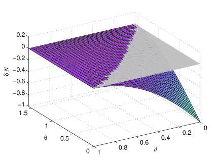
Figure 7: (Color online) $\delta N$ as a function of $d$ and $\theta$, where $\theta$ ranges from 0 to $\pi/2$.

As to $d_{3}>0$, we only consider $d_{3}$ is very small relative to $d$, due to the fact that qubit 3 is not transmitted remotely. That is to say, the ratio of $d_{3}$ to $d$ is far less than unit. On the other hand, it has been pointed out that if one selects a measurement angle $\theta^{\prime}$ which is close to but less than $\pi/2$, $N^{\prime}_{+}(\rho_{+})$ is larger than $N^{\prime}(\varrho)$ for almost the whole regime of $0<d<1$. Based on these considerations, we plot $\delta N$ as a function of $d$ and $r=d_{3}/d$ in Fig. 8 with $\theta\equiv\theta^{\prime}=1.5$ and $0\leqslant r\leqslant 0.1$. It can be seen that even when $d_{3}$ takes nonzero values, $N^{\prime}_{+}(\rho_{+})$ can be larger than $N^{\prime}(\varrho)$ for almost all values of $d$. It is worth pointing out that the increase in $d_{3}$ will lead to the increase in the probability $P_{+}$ of obtaining the state $\rho_{+}^{(12)}$ for a fixed $\theta$, because $P_{+}$ is proportional to the product of $d_{3}$ and $\cos\theta$ as given in Eq. (9). Now we can safely conclude that the aforementioned ADS is able to enhance, with a certain probability, the quality of bipartite entanglement distribution, compared to DDS in the above-mentioned case.

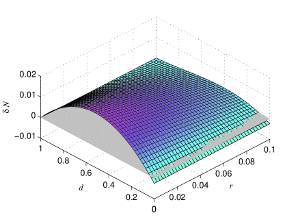
Figure 8: (Color online) $\delta N$ versus $d$ and $r$ ($=d_{3}/d$), where $r\in[0,0.1]$ and $\theta\equiv\theta^{\prime}=1/5$.

IV Concluding remarks

In summary, we have investigated the effect of quantum decoherence on the localization of a three-qubit GHZ state to a two-qubit entangled state. We used two different entanglement measures, negativity and FEF, to quantify the resulting bipartite entanglement after localization procedure. It turns out that the optimal measurement basis in the noise-free case is no more the optimal one under the amplitude noise. Moreover, the depolarizing noise has different influence from amplitude noise on the entanglement localization. The difference of the effects and the change of the optimal measurement bases justify the necessity of investigating the entanglement localization in various noisy environments. It has also been shown that the optimal measurement basis in the concept of localizable-entanglement does not match to the one for optimizing the practical applications of entanglement localization. Furthermore, we found that the idea of entanglement localizing could be used to probabilistically improve the equality of bipartite entanglement distribution. These findings shed new insights into entanglement manipulations and transformations, and provide a new idea of entanglement distributing against decoherence as well.

Although the results above are obtained from the case that the initial multipartite entangled resource is a three-qubit GHZ state, the conclusions could be directly generalized to the case involving $N$-qubit ($N>3$) GHZ states. It is deserved to research the effects of different types of quantum noises on entanglement localization and distribution for a variety of multipartite entangled states.

- (1) Horodecki R, Horodecki P, Horodecki M and Horodecki K 2009 Rev. Mod. Phys. 81 865-942
- (2) Pan J W, Chen Z B, Lu C Y, Weinfurter H, Zeilinger A and Żukowski M 2012 Rev. Mod. Phys. 84 777-838
- (3) Acín A, Cirac J I and Lewenstein M 2007 Nature Phys. 3 256-259
- (4) Kimble H J 2008 Nature 453 1023-1030
- (5) Perseguers S, Cirac J I, Acín A, Lewenstein M and Wehr J 2008 Phys. Rev. A 77 022308
- (6) DiVincenzo D P, et al, “The entanglement of assistance”, in Lecture Notes in Computer Science (Springer-Verlag, Berlin, 1999) 1509 247-257
- (7) Laustsen T, Verstraete F and van Enk S J 2003 Quantum Inf. and Comp. 3 64-83
- (8) Verstraete F, Popp M and Cirac J I 2004 Phys. Rev. Lett. 92 027901
- (9) Popp M, Verstraete F, Martin-Delgado M A and Cirac J I 2005 Phys. Rev. A 71 042306
- (10) Gour G 2006 Phys. Rev. A 74 052307
- (11) Clerk A A, Devoret M H, Girvin S M, Marquardt F and Schoelkopf R J 2010 Rev. Mod. Phys. 82 1155-1208
- (12) Aolita L, Chaves R, Cavalcanti D, Acín A and Davidovich L 2008 Phys. Rev. Lett. 100 080501
- (13) Man Z X, Xia Y J and An N B 2008 Phys. Rev. A 78 064301
- (14) Huang J H, Wang L G, and Zhu S Y 2010 Phys. Rev. A 81 064304
- (15) Zhou J and Guo H 2012 J. Phys. B: At. Mol. Opt. Phys. 45 225503
- (16) Perseguers S, Lapeyre Jr G J, Cavalcanti D, Lewenstein M and Acín A 2013 Rep. Prog. Phys. 76 096001.
- (17) Greenberger D M, Horne M A, Shimony A and Zeilinger A 1990 Am. J. Phys. 58 1131-43
- (18) Bose S, Vedral V and Knight P L 1998 Phys Rev A 57 822-29
- (19) Lu C Y, Yang T and Pan J W 2009 Phys Rev Lett 103 020501
- (20) Pagonis C, Redhead M L G, Clifton R K 1991 Phys. Lett. A 155 441-44
- (21) Hillery M, Bužek V and Berthiaume A 1999 Phys. Rev. A 59 1829-34
- (22) Xiao L, Long G L, Deng F G and Pan J W 2004 Phys. Rev. A 69 052307
- (23) Wang X W, Zhang D Y, Tang S Q and Gao F 2010 Int. J. Quantum Inf. 8 1301-14
- (24) Nielsen M and Chuang I, Quantum Computation and Quantum Information (Cambridge Univ. Press, Cambridge, 2000).
- (25) Zyczkowski K, Horodecki P, Sanpera A and Lewenstein M 1998 Phys. Rev. A 58 883-92
- (26) Vidal G and Werner R F 2002 Phys. Rev. A 65 032314
- (27) Bennett C H, DiVincenzo D P, Smolin J A and Wootters W K 1996 Phys. Rev. A 54 3824-51
- (28) Horodecki M, Horodecki P and Horodecki R 1999 Phys. Rev. A 60 1888-98
- (29) Bennett C H, Brassard G, Popescu S, Schumacher B, Smolin J A and Wootters W K 1996 Phys. Rev. Lett. 76 722-725
- (30) Horodecki M, Horodecki P and Horodecki R 1997 Phys. Rev. Lett. 78 574-77
- (31) Almeida M P, de Melo F, Hor-Meyll M, Salles A, Walborn S P, Souto Ribeiro P H and Davidovich L 2007 Science 316 579-82
- (32) Yu T and Eberly J H 2004 Phys. Rev. Lett. 93 140404
- (33) Laurat J, Choi K S, Deng H, Chou C W and Kimble H J 2007 Phys. Rev. Lett. 99 180504
- (34) Bellomo B, Lo Franco R and Compagno G 2007 Phys. Rev. Lett. 99 160502
- (35) Huang J H and Zhu S Y 2007 Phys. Rev. A 76 062322
- (36) Badziag P, Horodecki M, Horodecki P and Horodecki R 2000 Phys. Rev. A 62 012311
- (37) Bandyopadhyay S 2002 Phys. Rev. A 65 022302
- (38) Verstraete F and Verschelde H 2003 Phys. Rev. Lett. 90 097901
- (39) Bandyopadhyay S and Ghosh A 2012 Phys. Rev. A 86 020304(R)
- (40) Verstraete F and Verschelde H 2002 Phys. Rev. A 66 022307