Magnetic helicity of global field in cycles 23 and 24

Abstract

For the first time we reconstruct the magnetic helicity density of global axisymmetric field of the Sun using method proposed by Brandenburg et al. (2003) and Pipin et al. (2013b). To determine the components of the vector potential, we apply the gauge which is typically employed in mean-field dynamo models. This allows for a direct comparison of reconstructed helicity with the predictions from the mean-field dynamo models. We apply the method to two different data sets: the synoptic maps of line-of-sight (LOS) magnetic field from the Michelson Doppler Imager (MDI) on board of Solar and Heliospheric Observatory (SOHO) and vector magnetic field measurements from Vector Spectromagnetograph (VSM) on Synoptic Optical Long-term Investigations of the Sun (SOLIS) system. Based on the analysis of MDI/SOHO data, we find that in solar cycle 23 the global magnetic field had positive (negative) magnetic helicity in the northern (southern) hemisphere. This hemispheric sign asymmetry is opposite to helicity of solar active regions, but it is in agreement with the predictions of mean-field dynamo models. The data also suggest that the hemispheric helicity rule may have reversed its sign in early and late phases of cycle 23. Furthermore, the data indicate an imbalance in magnetic helicity between the northern and southern hemispheres. This imbalance seem to correlate with the total level of activity in each hemisphere in cycle 23. Magnetic helicity for rising phase of cycle 24 is derived from SOLIS/VSM data, and qualitatively, its latitudinal pattern is similar to the pattern derived from SOHO/MDI data for cycle 23.

1 Introduction

The generation of the magnetic field in the Sun is tightly related with the convective helical motions. In the framework of axisymmetric dynamos, the magnetic field is typically decomposed into toroidal and poloidal components. Parker (1955) suggested that solar dynamo can be represented as a periodic transformation of poloidal magnetic field, $\bar{\mathbf{B}}^{(p)}={\bar{B}}_{r}\mathbf{e}_{r}+{\bar{B}}_{\theta}\mathbf{e}_{\theta}$, into toroidal field $\bar{\mathbf{B}}^{(t)}={\bar{B}}_{\phi}\mathbf{e}_{\phi}$ (via the differential rotation) and the reverse transformation of $\bar{\mathbf{B}}^{(t)}$ to $\bar{\mathbf{B}}^{(p)}$ by helical convective motions. Further development of dynamo theory showed that the two processes produce helical magnetic fields on both small and large spatial scales (Frisch et al., 1975; Pouquet et al., 1975), and that the conservation of magnetic helicity is an important factor for the dynamical quenching of large-scale magnetic field generation (Kleeorin & Ruzmaikin, 1982; Cattaneo & Vainshtein, 1991; Vainshtein & Cattaneo, 1992; Kleeorin & Rogachevskii, 1999; Kleeorin et al., 2000; Brandenburg & Subramanian, 2005).

Early observations of various proxies of magnetic/current helicity established what is now known as the hemispheric helicity rule: magnetic fields of active regions exhibit preferentially negative (positive) helicity in the northern (southern) hemisphere (Seehafer, 1990; Pevtsov et al., 1995; Zhang et al., 2010, and references therein).

On the other hand, some researchers (e.g., Brandenburg et al., 2003; Blackman & Brandenburg, 2003; Warnecke et al., 2011; Pipin et al., 2013a, b) argued that magnetic helicity of large-scale (global) axisymmetric field should be positive/negative in the northern/southern hemisphere. Furthermore, the mean-field dynamo models predict reversals of the sign of helicity in association with the propagation of dynamo wave inside the convection zone (e.g., Warnecke et al., 2011; Pipin et al., 2013b). Reversals of the hemispheric helicity rule have been reported in observations, but the results seems inconclusive, with some researchers reporting the presence of such reversals in early/late phases of solar cycle (Bao et al., 2000; Hagino & Sakurai, 2005), while others are questioning their existence (Pevtsov et al., 2001, 2008; Gosain et al., 2013). Such apparent controversy may be resolved via direct comparison of observations with the model predictions. Since dynamo models can provide a detailed information about the distribution of magnetic helicity of global axisymmetric field in the convection zone and near the photosphere, it is highly desirable to directly compare these model estimates with the observations.

Theory suggests that magnetic helicity on small and large scales should have opposite sign (e.g., Pouquet et al., 1976; Seehafer, 1996; Blackman & Brandenburg, 2003; Brandenburg & Subramanian, 2005; Pipin et al., 2013a, b). Then, the small-scale helicity may dissipate on small spatial scales subject to the Ohmic dissipation (e.g., Pouquet et al., 1976) or the helicity of both signs could emerge through the solar photosphere. Early measurements of vertical component of large-scale current helicity density, (e.g., Pevtsov & Latushko, 2000; Wang & Zhang, 2010) found that in its sign, the large-scale magnetic fields follow the same hemispheric helicity rule as the active regions. These early studies concentrated on spatial scales larger than the active regions but smaller then the solar hemisphere. One should note that in the framework of mean-field dynamo, the magnetic fields of active regions represent the “small-scale” fields, while the large-scale fields refer to spatial scales comparable with the size of solar hemisphere. In this article, we address the helicity determination for large-scale magnetic fields as defined by mean-field dynamo theory. To avoid confusion with previous studies, we use the terms “global” and “large-scale” to refer to magnetic fields on spatial scales much larger then active regions. We reconstruct the magnetic helicity of global axisymmetric field using the approach suggested by Brandenburg et al. (2003) and Pipin et al. (2013b, see Section 2 below). Section 3 describes the data sets and the reduction procedure. Section 4 presents our main results, and in Section 5 we discuss our findings.

2 The formalism behind the computation of helicity of global axisymmetric field

Let us represent the axisymmetric magnetic field $\mathbf{\bar{B}}$ as

$$\bar{\mathbf{B}} = \mathbf{e_{\phi}}\bar{B}_{\phi}+\nabla\times\left(\bar{A}_{\phi}\mathbf{e_{\phi}}\right)=\nabla\times\bar{\mathbf{A}},$$ (1)

$$\bar{\mathbf{A}} = \mathbf{r}\bar{A}_{r}+\bar{A}_{\phi}\mathbf{e_{\phi}}=\mathbf{r}T+\nabla\times\left(\mathbf{r}S\right),$$ (2)

where, $\mathbf{r}=r\mathbf{e}_{r}$, $\nabla\times\left(\mathbf{r}\bar{A}_{r}\right)=\mathbf{e_{\phi}}\bar{B}_{\phi}$. Representation of the vector potential by equation (2) is often employed in mean-field dynamo models. In the spherical coordinates, the scalar functions $S$ (poloidal potential) and $T$ (toroidal potential), which are functions of $t$ (time), $r$ (radius), $\theta$ (polar angle) and $\phi$ (azimuth), are uniquely determined with the gauge (e.g., Krause & Rädler, 1980; Bigazzi & Ruzmaikin, 2004):

$$\int_{0}^{2\pi}\int_{-1}^{1}Sd\mu d\phi=\int_{0}^{2\pi}\int_{-1}^{1}Td\mu d\phi=0,$$ (3)

where $\mu=\cos\theta$. Equation (3) is time-dependent, and it is applicable to arbitrary $r$ including the solar surface at $r=R_{\sun}=R$. The magnetic helicity density is given by $\bar{\mathbf{A}}\cdot\bar{\mathbf{B}}$. In this study we concentrate on the axisymmetric magnetic field, and thus, ignore a dependence of magnetic field components on azimuth $\phi$.

Let us suppose that we have information about the axisymmetric components of the toroidal field, $\bar{B}_{\phi}$ and the poloidal field, $\bar{B}_{r}$ from the observations. Then, decomposing $r$ and $\phi$ components of magnetic field and its vector potential on series of the Legendre polynomial $P_{n}$ and $P_{n}^{1}$:

$$\bar{A}_{\phi}\left(t,\theta\right)=\sum_{n=1}^{N}a_{\phi}^{(n)}\left(t\right)P_{n}^{1}\left(\cos\theta\right),$$ (4)

$$\bar{B}_{r}\left(t,\theta\right)=\sum_{n=1}^{N}b_{r}^{(n)}\left(t\right)P_{n}\left(\cos\theta\right),$$ (5)

$$\bar{B}_{\phi}\left(t,\theta\right)=\sum_{n=1}^{N}b_{\phi}^{(n)}\left(t\right)P_{n}^{1}\left(\cos\theta\right),$$ (6)

$$\bar{A}_{r}\left(t,\theta\right)=\sum_{n=1}^{N}a_{r}^{(n)}\left(t\right)P_{n}\left(\cos\theta\right),$$ (7)

and using a known relation between $P_{n}$ and $P_{n}^{1}$,

$$P_{n}^{1}=-\sin\theta\frac{\partial P_{n}}{\partial\mu},\,-\frac{\partial P_{n}^{1}}{\partial\mu}=n\left(n+1\right)P_{n},$$

one can derive the following algebraic relations between the coefficients for magnetic field and the vector potential Legendre polynomial series:

$$a_{\phi}^{(n)}\left(t\right) = -\frac{Rb_{r}^{(n)}\left(t\right)}{n\left(n+1\right)},$$ (8)

$$a_{r}^{(n)}\left(t\right) = -Rb_{\phi}^{(n)}\left(t\right),$$ (9)

where $R$ is the radius of the Sun and $n$ is some finite (reasonably large) number. In the study we adopt n$\geq 48$.

The derivations of the vector potential and helicity in Brandenburg et al. (2003) are based on odd modes of equation (8). Here, we take into account both the radial and the toroidal magnetic fields, and we use information from both even and odd modes of the coefficients in equations (4-7). This approach allows us to study both symmetric (relative to the solar equator) and antisymmetric components of magnetic helicity density. To calculate a proxy for poloidal component of large-scale current helicity density, $\bar{B}_{r}\left(\nabla\times\mathbf{\bar{B}}\right)_{r}$, we employ the following identities:

$$\left(\nabla\times\bar{\mathbf{B}}\right)_{r}\left(t,\theta\right) = \sum_{n=1}^{N}\left(\nabla\times\bar{\mathbf{B}}\right)_{r}^{(n)}\left(t\right)P_{n}\left(\cos\theta\right),$$ (10)

$$\left(\nabla\times\bar{\mathbf{B}}\right)_{r}^{(n)}\left(t\right) = -\frac{n\left(n+1\right)b_{\phi}^{(n)}\left(t\right)}{R}$$ (11)

Scalar function $S$ (poloidal potential, see equation 2) can be determined within the uncertainty of a gauge (constant), which does not affect the vector potential of poloidal field (toroidal part of the vector potential $\mathcal{A}_{\phi}$). The gauge in equation (3) only affects the vector potential of the toroidal field (poloidal component of vector potential $\mathcal{A}_{r}$). This component of vectors potential is determined via equations (7,9). In the reconstruction of vector potential, equation(3) can be satisfied numerically by re-defining $\bar{A}_{r}(t,\mu)=\bar{A}_{r}^{(0)}(t,\mu)-\pi C(t)$, where $\bar{A}_{r}^{(0)}\left(t,\mu\right)={\displaystyle\sum_{n=1}^{N}a_{r}^{(n)}\left(t\right)P_{n}\left(\mu\right)}$ and $C$ can be determined numerically from the integration:

$$\int_{0}^{2\pi}\int_{-1}^{1}\bar{A}_{r}^{(0)}\left(t,\mu\right)d\mu d\phi=2\pi\int_{-1}^{1}\bar{A}_{r}^{(0)}\left(t,\mu\right)d\mu=C\left(t\right),$$ (12)

In the course of the reconstruction, we found that the amplitude of $C\left(t\right)$ is rather small in comparison with $\bar{A}_{r}^{(0)}(t,\mu)$. Equations (1–3,12) ensure that $\int_{-1}^{1}\bar{A}_{\phi}\bar{B}_{\phi}d\mu=\int_{-1}^{1}\bar{A}_{r}\bar{B}_{r}d\mu$ which should be expected from the topological considerations (see Section 4 and Brandenburg et al., 2003). Additional details about the formalism employed in computation of helicity of global field can be found in Pipin et al. (2013b).

3 Data reduction

3.1 The construction of maps

a)

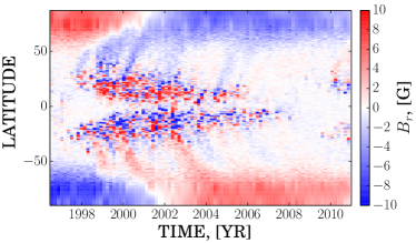
b)

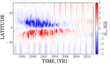
c)

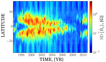
Figure 1: The time-latitude evolution of the large-scale magnetic field derived from MDI synoptic charts: a) the $\bar{B}_{r}$ component; b) the $\bar{B}_{\phi}$ component; the standard error of the $\bar{B}_{\phi}$. Vertical stripes in the toroidal flux and its error are the results of annual variations in the latitude of solar disk center (so called B₀–angle).

Next, we employed the synoptic maps of line-of sight (LOS) magnetic fields from the Solar and Heliospheric Observatory/Michelson Doppler Imager (SOHO/MDI) data set (Scherrer et al., 1995; Liu et al., 2004; Hoeksema et al., 2010; Sun et al., 2011). The $\bar{B}_{r}$ and $\bar{B}_{\phi}$ components of magnetic field are derived from a set of synoptic maps constructed using 10-degree wide longitudinal segments of solar disk image centred at the following longitudes relative to the central meridian: $\phi_{i}=0,\pm(15,30,45$^∘ and $60$${}^{\circ})$.

The poloidal and toroidal components of magnetic field can be determined following Duvall et al. (1979) approach, under the assumption that the observed changes in the magnetic fields over several days are entirely due to the change in the projection of the same magnetic field vector. Ideally, the method requires to compare the same feature on all images (see, Duvall et al., 1979; Grigoryev et al., 1986; Pevtsov & Latushko, 2000; Wang & Zhang, 2010). Instead, we employ a more simplified approach by comparing areas with the same latitudes and longitudes in synoptic maps constructed for different longitudinal offsets.

For each pixel on these synoptic maps of LOS field

$$B_{l}\left(t,\phi_{i},\theta\right)=\bar{B}^{\prime}_{r}\left(t,\theta\right)\sin\theta\cos\phi_{i}+\bar{B}_{\phi}\left(t,\theta\right)\sin\phi_{i},$$ (13)

where $B_{l}$ is the line-of-sight component of magnetic field and $\bar{B}^{\prime}_{r}$ and $\bar{B}_{\phi}$ are its radial (poloidal) and toroidal component of global magnetic field (here we introduce $\bar{B}^{\prime}_{r}$ notation to distinguish from $\bar{B}_{r}$ computed by SOHO/MDI team using a different approach). One can see that a simple addition/subtraction of synoptic maps taken with longitudinal offsets symmetric relative to the central meridian (e.g., $\pm$ 30^∘) allows to determine $\bar{B}^{\prime}_{r}$ and $\bar{B}_{\phi}$ from the equation 13. To lessen the effects of magnetic field evolution, we smooth each synoptic map by convolving it with a symmetric 2D Gaussian function with the FWHM of four solar degrees. Next, we determine the toroidal and poloidal components by fitting equation (13) for each Carrington longitude using the data taken with different longitudinal offsets. Finally, we average the obtained components of the magnetic field vector over each Carrington rotation to derive the latitudinal profiles of $\bar{B}^{\prime}_{r}$ and $\bar{B}_{\phi}$. As a test, we compared the $\bar{B}^{\prime}_{r}$ with $\bar{B}_{r}$ from the synoptic charts of radial solar magnetic field provided by the MDI team (Sun et al., 2011). We found that the latitudinal profiles of $\bar{B}^{\prime}_{r}$ derived by us agrees well with $\bar{B}_{r}$ profiles derived by SOHO/MDI team. Some minor deviations were found at very high latitudes near the polar regions. The latter could be explained by the fact that SOHO/MDI synoptic maps of radial ($\bar{B}_{r}$) field employ the polar field filling, while we employ $B_{l}$ synoptic charts without pole-filling. In further computations we use the latitudinal profiles of $\bar{B}_{r}$. As other test, for three solar rotations (CR1913, 1979, 2058), we compared the latitudinal profiles of radial and toroidal fields derived by us with those from Wang & Zhang (2010). We found a good agreement between two independent derivations.

Figure 1 demonstrates the derived distribution of radial and toroidal components of magnetic field for the entire SOHO/MDI data set. One can see several well-known patterns. For example, at high latitudes, the radial flux (Figure 1a) shows weak polar fields of correct sign, as well as the polar field reversals shortly after the maximum of cycle 23. In mid-latitudes, the prevailing polarity field is positive/negative in the northern/southern hemisphere, in agreement with the leading polarity of active region fields for cycle 23. As the leading polarity flux in active regions is more compact (and hence, may last longer) in comparison with the following polarity flux, average synoptic charts such as Figure 1 tend to emphasize the leading fields. The toroidal field (Figure 1b)in active region belts is negative/eastward in the northern hemisphere (and it is positive/westward in the southern hemisphere) in agreement with the prevailing polarity orientation of active regions in cycle 23 (i.e., Hale polarity rule). The data also show a weak (but persistent) pattern of east-west inclination of solar magnetic field, which is in agreement with Lo et al. (2010) and Sun et al. (2011) findings.

Figure 1b shows that at high latitude (near polar) regions there is a weak but persistent toroidal field oriented in opposite direction to the field of active regions. Thus, for example, weak fields in the declining phase of cycle 23 are oriented westward (positive)/eastward (negative) in the northern/southern hemisphere. In combination with the polarity of polar field in cycle 23, this implies that the weak fields outside of active regions are inclined (pointing towards) up-eastward in the southern hemisphere and down-westward in the northern hemisphere. Such tilt was previously noted by Duvall et al. (1979); Pevtsov & Latushko (2000). One could also note, that at high latitudes, the sign of the toroidal component of weak field corresponds to the orientation of active region magnetic fields in the next cycle 24 as if these weak fields herald the cycle 24 starting at high latitudes well before the first active region of this cycle emerges. Tlatov et al. (2010, 2013) found signs of the extended solar cycle in the orientation of ephemeral active regions several years prior to beginning of sunspot cycle, which qualitatively agrees with high latitude patterns shown in Figure 1.

3.2 Mitigation of orbital periodicity and the reduction of noise

Toroidal flux shows the effects related to a one year orbital periodicity and the presence of a noise component. To mitigate the effects of orbital periodicity, we employ the following strategy. Since the toroidal magnetic field and the toroidal vector potential should be zero at the poles, we restricted the computation of $\bar{B}_{\phi}$ to $\pm$70^∘ latitudes. For latitudes between 70^∘ and 90^∘ the toroidal field was extrapolated linearly from lower latitudes.

Noise in toroidal flux was reduced by convolving the data (Figure 1) with 2D Gaussian function:

$$G(\mu,t)=\exp\left(-\frac{\mu^{2}}{2b^{2}}\right)\left[\exp\left(-\frac{t^{2}}{2a^{2}}\right)-e^{-2}\left(3-\frac{t^{2}}{2a^{2}}\right)\right],$$ (14)

where $t$ is a discrete time given in units of Carrington rotations (CR). The data are defined at the homogeneous mesh in $\mu$. For spatial $\mu$ coordinate we employ the filter with the full width at half maximum (FWHM) to be equal to 20 points of mesh, which corresponds to $b\approx 0.04$ in equation 14. For time coordinate, the FWHM is equal to 24 CR, i.e, $a=12$ CR. In addition, we apply reflection conditions at the boundaries for spatial component of filter and vanishing first derivative at the end-points for the time component of the filter (second term in square brackets in equation 14). Similar filter is usually applied for sunspot number analysis (Hathaway, 2009).

3.3 The derivation of vector potentials

Figure 2 shows the derived symmetric and asymmetric (relative to equator) components of radial and toroidal magnetic fields. (One can note that the amplitude of solar cycle variations in symmetric components is smaller as compared with the asymmetric one. We postpone the discussion of this till Section 4.) Following Zhang et al. (2010), the window sizes of temporal and spatial scales involved in equation (14) are chosen to correspond to the scales of turbulent diffusion (we thanks K.M. Kuzanyan for this idea), which is about $10^{12}$cm${}^{2}/$sec (Abramenko et al., 2011).

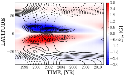
a)b)

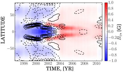
Figure 2: The time-latitude variations of the toroidal (background image), $\bar{B}_{\phi}$, and the radial field, $\bar{B}_{r}$ (contours), after convolution with kernel defined by equation (14). Panels (a) and (b) show asymmetric and symmetric components of magnetic field, accordingly. Positive (solid) and negative (dashed) contours are drawn at equal steps in amplitude of $\bar{B}_{r}$ within the range of $\pm 6$G (panel a) and $\pm$3G.

Next, we interpolate the data to the collocation points of the Legendre polynomials, $\mu_{j}=\cos\theta_{j}$, which are taken at zeros of $P_{n}\left(\mu\right)$. The order of the polynomial approximation, n, should be sufficiently high. We found that the results do not change significantly for $n\geq 48$, which was the basis for selecting N$=$48 as upper limit for summation in equation 15. The coefficients $a_{\phi}^{(n)}(t)$ in equation(4) can be found using the equation(1) and properties of the Legendre polynomials. The matrix equation for $a_{\phi}^{(n)}\left(t\right)$ becomes

$$R\bar{B}_{r}\left(t,\mu_{j}\right) = -\sum_{n=1}^{N}a_{\phi}^{(n)}\left(t\right)n\left(n+1\right)P_{n}\left(\mu_{j}\right),$$ (15)

$$\bar{B}_{\phi}\left(t,\mu_{j}\right) = \sum_{n=1}^{N}b_{\phi}^{(n)}\left(t\right)P_{n}^{1}\left(\mu_{j}\right).$$ (16)

By solving the matrix equations in the collocation points, one can find the coefficients for the vector potential components and restore the distribution of magnetic helicity density. The validity of this reconstruction procedure was tested using the output of a mean-field dynamo model of Pipin et al. (2013b).

The main conclusions of this paper are drawn from the analysis based on LOS magnetic field synoptic maps. These maps cover the solar cycle 23 and the beginning of cycle 24. In addition, for the rising phase of solar cycle 24 we employed the vector synoptic maps from Vector Spectromagnetograph (VSM) on Synoptic Optical Long-term Investigations of the Sun (SOLIS) system (Gosain et al., 2013). The maps cover 20 consecutive solar rotations starting from the CR2109; this data set covers the period from March 2011 to December 2012. Time-latitude distribution of radial and toroidal components of vector magnetic field are shown in Figure 3(a,b). Figure 3(c) shows the average latitudinal profiles of two components of axisymmetric large-scale magnetic field. The profiles were obtained by averaging over the Carrington rotations 2109–2128 and applying the Gaussian filter with FWHM equal 30 pixels in sine of latitude.

a)

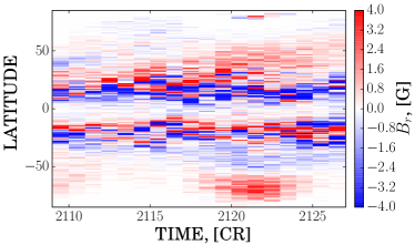
b)

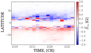
c)

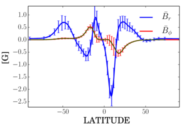
Figure 3: Radial ($\bar{B}_{r}$, panel a) and toroidal ($\bar{B}_{\phi}$, panel b) magnetic fields derived from SOLIS/VSM synoptic vector charts. Panel (c) shows the mean latitudinal profiles of $\bar{B}_{r}$ and $\bar{B}_{\phi}$ together with the 90 % confidence interval.

While there is no overlap between the MDI and VSM datasets to allow for a more direct comparison, we note that the distributions of radial and toroidal fields from two data sets exhibit somewhat similar behavior. For example, similar to Figure 1 mean toroidal field derived from the vector data is mostly negative in the northern hemisphere, and it is mostly positive in the southern hemisphere. The polarity of radial field in the main peak (negative in the northern hemisphere and positive in the southern hemisphere) corresponds to the leading and following polarity fields of dissipating active regions. MDI data (Figure 1a) show similar patterns in some parts of cycles 23 and 24 (e.g., see “tip” of cycle 24 “butterfly” in the northern hemisphere). These general similarities provide some level of confidence for our method of derivation of radial and toroidal components of large-scale magnetic field from MDI synoptic maps of LOS flux.

4 Results

Figure 4(a,b) presents the evolution of power spectra $\sqrt{\left[b_{\phi}^{(n)}\left(t\right)\right]^{2}}$ and $\sqrt{\left[a_{\phi}^{(n)}\left(t\right)\right]^{2}}$. The coefficients $b_{\phi}^{(n)}\left(t\right)$ and $a_{\phi}^{(n)}\left(t\right)$ decay rapidly with the increasing number of modes. Furthermore, we found that the asymmetric component of the magnetic field exhibits a faster decay, which we interpret as if this component being more global in its nature as compared with the symmetric component. In a hindsight, we note that one can draw a similar conclusion using the results of Stenflo & Guedel (1988) study.

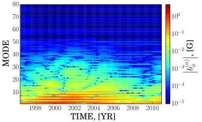
a)b)

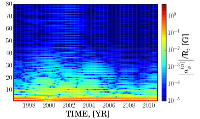
Figure 4: The evolution of power spectra, $\sqrt{\left[b_{\phi}^{(n)}\left(t\right)\right]^{2}}$ (panel a) and $\sqrt{\left[a_{\phi}^{(n)}\left(t\right)\right]^{2}}$ (panel b).

Figure 5 shows the reconstructed components of vector potential which are computed for two cases: (1) taking into account odd and even modes of the spectral harmonics and (2) including only the even modes (associated with the asymmetric part of global magnetic field). There, we used the first 11 modes in equations (4,7). Restricting the expansion to 11 modes is well-justified by a rapid decay of $a^{(n)}\left(t\right)$ for higher modes (Figure 4b).

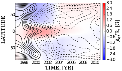
a)b)

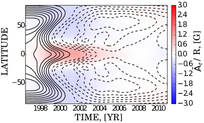
Figure 5: Radial ($\bar{A}_{r}/R$, background images) and toroidal ($\bar{A}_{\phi}/R$, contours) components of vector potential for (a) case 1 (including both odd and even modes) and (b) case 2 (only even modes). Positive (solid) and negative (dashed) contours are drawn at equal steps in amplitude of $\bar{A}_{\phi}/R$ within the range of $\pm 2$G.

The pattern of symmetric (relative to the equator) component of $\bar{A}_{\phi}$ is similar in appearance to reconstruction made by Brandenburg et al. (2003) based on Stenflo & Guedel (1988) data. Note, that in our case we don’t restrict the study to a particular symmetry of the global field about the equator. We find that the poloidal component of vector potential (Figure 5a) exhibits a break in the equatorial symmetry (see change in sign of $\bar{A}_{r}$ around year 2004). The asymmetry between northern and southern hemispheres is also present at high latitudes prior to year 1998. On the other hand, the pattern of the $\bar{A}_{\phi}$ (Figure 5b) exhibits no significant changes over the solar cycle 23.

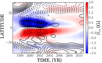
a)b)

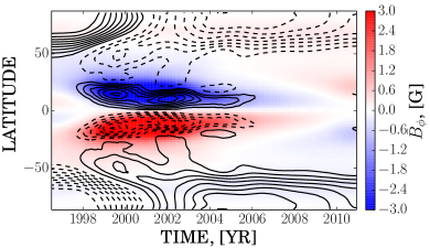
Figure 6: Radial ($\bar{B}_{r}$, contours) and toroidal ($\bar{B}_{\phi}$, background images) components of large-scale magnetic field for (a) case 1 (odd and even modes) and (b) case 2 (even modes, only) computed using first 11 modes in the equations (5,6). Positive (solid) and negative (dashed) contours are drawn at equal steps in amplitude of within the range of $\pm 6$G.

Figure 6 shows the components of the large-scale magnetic field. There, again, we use the first 11 modes in equations (5,6). The obtained evolution of $\bar{{B}}_{r}$ is in agreement with results of Ulrich & Tran (2013). The pattern of $\bar{{B}}_{\phi}$ in Figure 5b (even modes) closely resembles Figure 2a. We also find that the phase relation $\bar{B}_{r}\bar{B}_{\phi}<0$ holds in equatorial region (see also, Stix, 1976; Yoshimura, 1976). Brandenburg et al. (2003) argued that this relation is tightly related with the sign of the magnetic helicity density. Figure 7 supports this conjecture for the asymmetric (relative to solar equator) part of the magnetic helicity density.

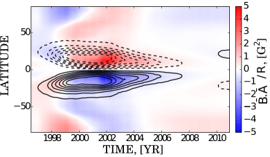
a)b)

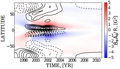
Figure 7: The magnetic helicity density for the asymmetric (relative to solar equator) part of the large-scale magnetic field. The panel a) shows the $\bar{\boldsymbol{\mathbf{A}}}\cdot\bar{\mathbf{B}}$ (background images) and the toroidal magnetic field (contours are within the range of $\pm 3$G); b) for the same case, the $\bar{A}_{\phi}\bar{B}_{\phi}/R$ (background images) and the $\bar{A}_{r}\bar{B}_{r}/R$ (contours are within the range of $\pm 5$G), both values vary within the same range of magnitude.

Having the radial and toroidal components of magnetic field and vector potential, we are now able to compute the corresponding contributions to magnetic helicity density $\bar{\boldsymbol{\mathbf{A}}}\cdot\bar{\mathbf{B}}=\bar{A}_{\phi}\bar{B}_{\phi}+\bar{A}_{r}\bar{B}_{r}$. The distribution of magnetic helicity density in cycle 23 (Figure 7a) shows a strong hemispheric asymmetry, with positive/negative helicity in the northern/southern hemispheres. This hemispheric asymmetry is opposite in sign to the hemispheric helicity rule found in active regions. There is no contradiction here. In the dynamo theory, the active regions are thought to represent the “small-scale” magnetic fields (see Brandenburg et al., 2003, for further discussion), while in this paper we derive helicity of large-scale fields (in mean-field dynamo terminology). The fact that large-scale helicity derived by us has an opposite sign to helicity of active regions is in agreement with the notion that the dynamo produces helicity of two opposite signs segregated by their spatial scales.

Patterns of toroidal ($\bar{A}_{\phi}\bar{B}_{\phi}$) and radial ($\bar{A}_{r}\bar{B}_{r}$) components of magnetic helicity density are quite different (Figure 7b). Comparing Figure 7 and Figure 8a we conclude that the total helicity in polar regions is defined by $\bar{A}_{r}\bar{B}_{r}$ contribution. In equatorial regions, both $\bar{A}_{r}\bar{B}_{r}$ and $\bar{A}_{\phi}\bar{B}_{\phi}$ have the same sign. Despite the difference in spatial distributions of $\bar{A}_{r}\bar{B}_{r}$ and $\bar{A}_{\phi}\bar{B}_{\phi}$, their total surface integrals are about equal ($\int\bar{A}_{\phi}\bar{B}_{\phi}d\mu=\int\bar{A}_{r}\bar{B}_{r}d\mu$), as verified by direct computations using our data (for a mathematical derivation of this equality, see Appendix). Therefore, one can compute the total surface helicity, $\mathcal{H}_{S}=\int\bar{\boldsymbol{\mathbf{A}}}\cdot\bar{\mathbf{B}}d\mu$, using only one of two parts as suggested by Brandenburg et al. (2003). The estimation of $\mathcal{H}_{S}$ separately for the northern and southern hemispheres still requires both $\bar{A}_{r}$ and $\bar{A}_{\phi}$.

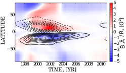
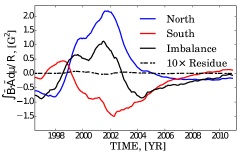
a) b) c)

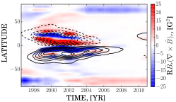
Figure 8: Magnetic helicity density (background image) and the large-scale toroidal field (contours, panel (a), and magnetic helicity density integrated over each hemisphere (panel b). Contribution from the modes with number larger than 11 is shown as “residue”. Panel (c) show current helicity density (background image) and the large-scale toroidal field (contours). Contours are drawn for the same levels as in Figure 7.

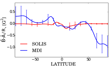
a)b)

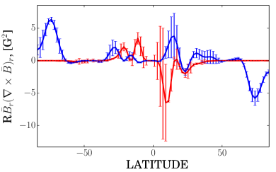
Figure 9: Latitudinal profiles of magnetic helicity density (a) and current helicity density (b) for SOLIS and MDI data sets. The 90 % confidence intervals are shown as error bars.

Modern measurements of solar vector magnetic fields are normally restricted to a single layer in solar atmosphere (typically, the photosphere). These observations are insufficient to derive the true magnetic helicity. Instead, various proxies of helicity are used. Figure 8c shows evolution of one of these helicity proxies, the radial component of current helicity density, $\bar{B}_{r}\left(\nabla\times\bar{\mathbf{B}}\right)_{r}$. In comparison with true magnetic helicity density (Figure 8a), $\bar{B}_{r}\left(\nabla\times\bar{\mathbf{B}}\right)_{r}$ shows a more complex pattern. While on average the current helicity density follows the same hemispheric sign-asymmetry as the magnetic helicity density, during the maximum of solar cycle 23 the $\bar{B}_{r}\left(\nabla\times\bar{\mathbf{B}}\right)_{r}$ exhibits a distinct “zebra” pattern with opposite helicity bands present in both hemispheres. Whatever these bands persist through the minimum of cycle 23 is not clear as our data are insufficient to make a definite conclusion about this. Similar “zebra” patterns in the $\bar{B}_{r}\left(\nabla\times\bar{\mathbf{B}}\right)_{r}$ were found in the past (e.g., Pevtsov & Latushko, 2000; Pevtsov & Balasubramaniam, 2003; Gosain et al., 2013). Pevtsov & Balasubramaniam (2003) speculated about a possible relation between the latitudinal bands of current helicity density and the subphotospheric pattern of torsional oscillations.

Figure 9 compares latitudinal profiles of $\bar{\boldsymbol{A}}\cdot\bar{\mathbf{B}}$ and $\bar{B}_{r}\left(\nabla\times\bar{\mathbf{B}}\right)_{r}$ computed using data from SOHO/MDI (about year 2011) and SOLIS/VSM (Figure 3c, year 2012). The 90 % confidence interval was computed in the same manner as for data shown in Figures 1c and 3c. The residual contribution of modes higher that n=11 (equations(4–7)) is an order of magnitude smaller then the contribution of first 11 modes. While both magnetic helicity density and $\bar{B}_{r}\left(\nabla\times\bar{\mathbf{B}}\right)_{r}$ exhibit the hemispheric helicity rule in both datasets, there are some differences. For example, the latitudinal profiles of helicity can differ because of evolutionary changes (MDI and VSM data included in this comparison correspond to periods, which are about one year apart). Other sources of difference could include difference in sensitivity to magnetic field and the noise levels, as well as the treatment of polar fields.

5 Discussion and Conclusions

Using synoptic charts from SOHO/MDI, we, for the first time, reconstruct the magnetic helicity density of global axisymmetric field of the Sun. In solar cycle 23 the global axisymmetric magnetic field exhibits positive magnetic helicity in the northern hemisphere, and negative one in the southern. In general, such reconstructions require a knowledge of the $\bar{B}_{r}$ and $\bar{B}_{\phi}$ components of the axisymmetric magnetic field. In the past, vector global magnetic field components were reconstructed via various approaches (Pevtsov & Latushko, 2000; Ulrich & Boyden, 2005; Lo et al., 2010; Mordvinov et al., 2012). Here we used synoptic charts of LOS magnetic field corresponding to different longitudinal offsets relative to central meridian to compute $\bar{B}_{r}$ and $\bar{B}_{\phi}$, see equation (13). Derived $\bar{B}_{r}$ agrees well with the $\bar{B}_{r}$ provided by the MDI team, which we see as indirect validation of our method.

Based on the analysis of dynamo equations, Brandenburg et al. (2003) suggested that the magnetic helicity of global magnetic field in solar cycle 23 should be positive/negative in the northern/southern hemisphere. Pipin et al. (2013b) analyzed the distributions of magnetic helicity for large- and small-scale magnetic fields in the axisymmetric mean-field dynamo taking into account the conservation of the total magnetic helicity in the dynamo processes. They concluded (see their Figures 2e,d and 5) that magnetic helicity density of large-scale field should have positive sign in the northern hemisphere and negative sign in the southern hemisphere during the most part of the magnetic cycle. Our present results provide observational support to these early theoretical predictions. We find that during most of cycle 23, global magnetic fields exhibited a persistent pattern of positive/negative helicity in the northern/southern hemispheres.

In respect to helicity of active region magnetic fields (small-scale in the framework of this discussion), the hemispheric helicity rule is negative/positive in the northern/southern hemispheres (Seehafer, 1990; Pevtsov et al., 1995; Zhang et al., 2010, and references therein). Taken together, these two results support the notion that the solar dynamo creates helicity of two opposite signs as was suggested in early papers. However, helicity of both signs seem to cross the solar photosphere. We further found that the hemispheric helicity rule for global magnetic fields exhibits sign-reversals in early and late phases of cycle 23. If the helicities of small- and large-scale fields are tied together, this should imply a need for similar reversals in the hemispheric helicity rule for active regions. Alas, while some researchers claimed observing reversals in the hemispheric helicity rule near the minimum of solar cycle 22 and 23 (Bao et al., 2000; Hagino & Sakurai, 2005), others were not able to find them (Pevtsov et al., 2001, 2008; Gosain et al., 2013). Clearly, this question about possible reversals of the hemispheric helicity rule for active region magnetic fields needs to be re-examined. Although, the predictions of the model by Pipin et al. (2013b) agree qualitatively with the results reported in our paper, there are some differences related to the shape of the helicity density patterns. For example, our present results suggest that magnetic helicity density pattern of the same sign can extend from the equator to the poles which is not seen in the model. Similarly, the pattern of $\bar{\mathbf{A}}\cdot\bar{\mathbf{B}}$ of reverse sign penetrates to equatorial regions during the minima of cycle around year 1997 and 2009. If the reversals of the hemispheric helicity rule are real, this will pose a challenge for some proposed mechanisms of helicity generation (e.g., helicity generation by the differential rotation, Berger & Ruzmaikin, 2000).

As an alternative explanation, our results could be interpreted in the framework of helicity of axisymmetric and non-axisymmetric parts of global magnetic fields. In that model, the axisymmetric component of helicity (derived in this article) follows the hemispheric helicity rule of opposite in sign to the non-axisymmetric component (associated with active regions). Such a possibility was raised by Zhang (2006), who used Berger & Ruzmaikin (2000) data to show that helicity flux of non-axisymmetric modes was opposite in sign to helicity of axisymmetric (m=0) mode.

One may also question the importance of vector magnetic field measurements for studies of global helicity, when the line-of-sight data seem to provide reasonable results. Here we presented the first ever derivations of magnetic helicity density of global field based on vector synoptic maps. While we see similarities in distribution of global helicity derived from LOS and vector data, there are also some differences. For example, synoptic maps of toroidal field derived from LOS data show more or less uniform distribution of the magnetic field polarity of one sign suggested by the the Hale polarity law. In addition to that pattern, vector field maps show mix of two different polarities: one is more concentrated and other is somewhat diffused (Figure 3b). The diffuse component (of toroidal field) seems to correspond to a trailing polarity field. Such component of large-scale field is not present in the maps of toroidal flux derived from the LOS magnetic fields. The vector field data are limited to cycle 24, and thus, are insufficient to conclude if there are any changes in this diffuse component of toroidal field with solar cycle. This and other differences between derivations based on LOS or vector field data require further investigation.

Our findings indicate that helicity of the large-scale magnetic fields is imbalanced between the northern and the southern hemispheres in different phases of solar cycle. However, when taken over the entire cycle, the positive and negative helicity of large-scale magnetic field is well-balanced. Indirectly, this is in agreement with Georgoulis et al. (2009), who found that helicity injection through the solar photosphere associated with active region magnetic fields is well-balanced over the solar cycle 23. On the other hand, Yang & Zhang (2012) reported significant imbalance between helicity fluxes of northern and southern hemispheres. Our findings (Figure 8c) allow to reconcile Georgoulis et al. (2009) and Yang & Zhang (2012) conclusions.

Due to limitations of the existing datasets, the observational studies of helicity often refer to proxies of current helicity density. It is usually assumed that these proxies represent magnetic helicity sufficiently well. Contrary to that, we find that while the general tendencies are similar in magnetic and current helicity densities, there are differences, for example, in small-scale patterns, which may be present in one helicity proxy but are absent in the other. For example, proxy of current helicity, $\bar{B}_{r}\left(\nabla\times\bar{\mathbf{B}}\right)_{r}$, exhibits a distinct “zebra” pattern, but no such pattern is present in the distribution of magnetic helicity. Early, Pevtsov & Latushko (2000) and Gosain et al. (2013) reported similar pattern in current helicity density of large-scale magnetic fields. The pattern could also be expected from spatial structure of the dynamo wave of the large-scale magnetic field components $\bar{B}_{r}$ and $\bar{B}_{\phi}$, which are illustrated in Figure 5a. We note that in the equatorial regions the inequality $\bar{B}_{r}\bar{B}_{\phi}<0$ holds for the most part of the sunspot cycle (see, Figure 5a). We also found that modes $b_{r}^{(3)}$ and $b_{\phi}^{(2)}$ dominate, which means that $\bar{B_{r}}\left(\boldsymbol{\nabla}\times\mathbf{\bar{B}}\right)_{r}\sim b_{\phi}^{(2)}b_{r}^{(3)}P_{2}P_{3}$, here the sign of the $b_{\phi}^{(2)}b_{r}^{(3)}$ defines the hemispheric sign rule and the product $P_{2}P_{3}$ defines that zebra pattern as illustrated in Figure 8c and Figure 9. Thus, the results shown in Figure 8c are expected for any dynamo model that qualitatively reproduces Figure 5a.

Finally, keeping in mind the approximations which were used in the reconstruction of components of the global magnetic field of the Sun, our results should be considered as preliminary. Further development in this direction is likely to shed more light on the role of magnetic helicity in global solar and astrophysical dynamos.

6 Appendix A

The components of large-scale axisymmetric field and the components of its vector potential are related with equations:

$$\bar{B}_{r} = -\frac{1}{r}\frac{\partial\left(\sin\theta\bar{A}_{\phi}\right)}{\partial\mu},$$ (A1)

$$\bar{B}_{\phi} = \frac{\sin\theta}{r}\frac{\partial\bar{A}_{r}}{\partial\mu},$$ (A2)

where $\mu=\cos\theta$. Then, using integration by part, we obtain:

$$\int_{-1}^{1}\bar{A}_{\phi}\bar{B}_{\phi}d\mu = \int_{-1}^{1}\frac{\sin\theta\bar{A}_{\phi}}{r}\frac{\partial\bar{A}_{r}}{\partial\mu}d\mu$$

$$= \left.\frac{\sin\theta\bar{A}_{\phi}\bar{A}_{r}}{r}\right|_{0}^{\pi}-\int_{-1}^{1}\frac{\bar{A}_{r}}{r}\frac{\partial\sin\theta\bar{A}_{\phi}}{\partial\mu}d\mu$$

$$= \int_{-1}^{1}\bar{A}_{r}\bar{B}_{r}d\mu.$$

References

- Abramenko et al. (2011) Abramenko, V. I., Carbone, V., Yurchyshyn, V., Goode, P. R., Stein, R. F., Lepreti, F., Capparelli, V., & Vecchio, A. 2011, ApJ, 743, 133
- Bao et al. (2000) Bao, S. D., Ai, G. X., & Zhang, H. Q. 2000, J. Astrophysics and Astronomy, 21, 303
- Berger & Ruzmaikin (2000) Berger, M. A., & Ruzmaikin, A. 2000, J. Geophys. Res., 105, 10481
- Bigazzi & Ruzmaikin (2004) Bigazzi, A., & Ruzmaikin, A. 2004, ApJ, 604, 944
- Blackman & Brandenburg (2002) Blackman, E. G., & Brandenburg, A. 2002, Astrophys. J., 579, 379
- Blackman & Brandenburg (2003) Blackman, E. G., & Brandenburg, A. 2003, ApJ, 584, L99
- Brandenburg et al. (2003) Brandenburg, A., Blackman, E. G., & Sarson, G. R. 2003, Advances in Space Research, 32, 1835
- Brandenburg & Subramanian (2005) Brandenburg, A., & Subramanian, K. 2005, Phys. Rep., 417, 1
- Cattaneo & Vainshtein (1991) Cattaneo, F., & Vainshtein, S. I. 1991, ApJ, 376, L21
- Duvall et al. (1979) Duvall, Jr., T. L., Scherrer, P. H., Svalgaard, L., & Wilcox, J. M. 1979, Sol. Phys., 61, 233
- Frisch et al. (1975) Frisch, U., Pouquet, A., Léorat, J., & A., M. 1975, J. Fluid Mech., 68, 769
- Georgoulis et al. (2009) Georgoulis, M. K., Rust, D. M., Pevtsov, A. A., Bernasconi, P. N., & Kuzanyan, K. M. 2009, ApJ, 705, L48
- Gosain et al. (2013) Gosain, S., Pevtsov, A. A., Rudenko, G. V., & Anfinogentov, S. A. 2013, ApJ, 772, 52
- Grigoryev et al. (1986) Grigoryev, V. M., Latushko, S. M., & Peshcherov, V. S. 1986, Contributions of the Astronomical Observatory Skalnate Pleso, 15, 481
- Hagino & Sakurai (2005) Hagino, M., & Sakurai, T. 2005, PASJ, 57, 481
- Hathaway (2009) Hathaway, D. 2009, Space Science Reviews, 144, 401, 10.1007/s11214-008-9430-4
- Hoeksema et al. (2010) Hoeksema, J. T., Liu, Y., Sun, X., & Zhao, X. 2010, AGU Fall Meeting Abstracts, D2
- Hubbard & Brandenburg (2012) Hubbard, A., & Brandenburg, A. 2012, ApJ, 748, 51
- Kleeorin et al. (2000) Kleeorin, N., Moss, D., Rogachevskii, I., & Sokoloff, D. 2000, A&A, 361, L5
- Kleeorin & Rogachevskii (1999) Kleeorin, N., & Rogachevskii, I. 1999, Phys. Rev.E, 59, 6724
- Kleeorin & Ruzmaikin (1982) Kleeorin, N. I., & Ruzmaikin, A. A. 1982, Magnetohydrodynamics, 18, 116
- Krause & Rädler (1980) Krause, F., & Rädler, K.-H. 1980, Mean-Field Magnetohydrodynamics and Dynamo Theory (Berlin: Akademie-Verlag), 271
- Kuzanyan et al. (2000) Kuzanyan, K., Zhang, H., & Bao, S. 2000, Solar Phys., 191, 231
- Liu et al. (2004) Liu, Y., Zhao, X., & Hoeksema, J. T. 2004, Sol. Phys., 219, 39
- Lo et al. (2010) Lo, L., Hoeksema, J. T., & Scherrer, P. H. 2010, in Astronomical Society of the Pacific Conference Series, Vol. 428, SOHO-23: Understanding a Peculiar Solar Minimum, ed. S. R. Cranmer, J. T. Hoeksema, & J. L. Kohl, 109
- Mordvinov et al. (2012) Mordvinov, A. V., Grigoryev, V. M., & Peshcherov, V. S. 2012, Sol. Phys., 280, 379
- Parker (1955) Parker, E. 1955, Astrophys. J., 122, 293
- Pevtsov et al. (1995) Pevtsov, A. A., Canfield, R. C., & Metcalf, T. R. 1995, ApJ, 440, L109
- Pevtsov & Balasubramaniam (2003) Pevtsov, A. A., & Balasubramaniam, K. S. 2003, Advances in Space Research, 32, 1867
- Pevtsov et al. (2001) Pevtsov, A. A., Canfield, R. C., & Latushko, S. M. 2001, ApJ, 549, L261
- Pevtsov et al. (2008) Pevtsov, A. A., Canfield, R. C., Sakurai, T., & Hagino, M. 2008, ApJ, 677, 719
- Pevtsov & Latushko (2000) Pevtsov, A. A., & Latushko, S. M. 2000, ApJ, 528, 999
- Pipin et al. (2013a) Pipin, V. V., Sokoloff, D. D., Zhang, H., & Kuzanyan, K. M. 2013a, ApJ, 768, 46
- Pipin et al. (2013b) Pipin, V. V., Zhang, H., Sokoloff, D. D., Kuzanyan, K. M., & Gao, Y. 2013b, MNRAS, 435, 2581
- Pouquet et al. (1975) Pouquet, A., Frisch, U., & Léorat, J. 1975, J. Fluid Mech., 68, 769
- Pouquet et al. (1976) Pouquet, A., Frisch, U., & Leorat, J. 1976, J. Fluid Mech., 77, 321
- Scherrer et al. (1995) Scherrer, P. H., et al. 1995, Sol. Phys., 162, 129
- Seehafer (1990) Seehafer, N. 1990, Sol. Phys., 125, 219
- Seehafer (1996) Seehafer, N. 1996, Phys. Rev. E, 53, 1283
- Stenflo & Guedel (1988) Stenflo, J. O., & Guedel, M. 1988, A&A, 191, 137
- Stix (1976) Stix, M. 1976, Astron. Astrophys., 47, 243
- Sun et al. (2011) Sun, X., Liu, Y., Hoeksema, J. T., Hayashi, K., & Zhao, X. 2011, Sol. Phys., 270, 9
- Tlatov et al. (2010) Tlatov, A. G., Vasil’eva, V. V., & Pevtsov, A. A. 2010, ApJ, 717, 357
- Tlatov et al. (2013) Tlatov, A. G., Illarionov, E., Sokoloff, D. D. & Pipin, V. V. 2013, MNRAS, 432, 2975
- Tiwari et al. (2009) Tiwari, S. K., Venkatakrishnan, P., & Sankarasubramanian, K. 2009, ApJ, 702, L133
- Ulrich & Boyden (2005) Ulrich, R. K., & Boyden, J. E. 2005, ApJ, 620, L123
- Ulrich & Tran (2013) Ulrich, R. K., & Tran, T. 2013, ApJ, 768, 189
- Vainshtein & Cattaneo (1992) Vainshtein, S. I., & Cattaneo, F. 1992, ApJ, 393, 165
- Wang & Zhang (2010) Wang, C., & Zhang, M. 2010, ApJ, 720, 632
- Warnecke et al. (2011) Warnecke, J., Brandenburg, A., & Mitra, D. 2011, A&A, 534, A11
- Yang & Zhang (2012) Yang, S., & Zhang, H. 2012, ApJ, 758, 61
- Yoshimura (1976) Yoshimura, H. 1976, Sol. Phys., 50, 3
- Zhang et al. (2010) Zhang, H., Sakurai, T., Pevtsov, A., Gao, Y., Xu, H., Sokoloff, D. D., & Kuzanyan, K. 2010, MNRAS, 402, L30
- Zhang (2006) Zhang, M. 2006, ApJ, 646, L85