Coincidence Landscapes for Three-Channel Linear Optical Networks

Abstract

We use permutation-group methods plus SU(3) group-theoretic methods to determine the action of a three-channel passive optical interferometer on controllably delayed single-photon pulse inputs to each channel. Permutation-group techniques allow us to relate directly expressions for rates and, in particular, investigate symmetries in the coincidence landscape. These techniques extend the traditional Hong-Ou-Mandel effect analysis for two-channel interferometry to valleys and plateaus in three-channel interferometry. Our group-theoretic approach is intuitively appealing because the calculus of Wigner $D$ functions partially accounts for permutational symmetries and directly reveals the connections among $D$ functions, partial distinguishability, and immanants.

I Introduction

Passive quantum optical interferometry aims to inject classical or nonclassical light into a multichannel interferometer and count photons exiting the output ports or measure coincidences at the exits Hong et al. (1987); Campos (2000) or even measure some outputs to perform post selection of the remaining output state. This post selection procedure is a key element of the nonlinear sign gate for optical quantum computing Knill et al. (2001) and for enhancement of the efficiency of single photons Berry et al. (2004a, b) or of single-rail optical qubits Berry et al. (2006). Another rapidly growing experimental direction in passive quantum optical interferometry is quantum walks Broome et al. (2010); Schreiber et al. (2011, 2012), which are being extended to two-photon inputs for two-walker quantum walks Sansoni et al. (2012).

The Hong-Ou-Mandel dip involves directing two identical photons such that one enters each of the two balanced (50:50) beam splitter inputs with a controllable relative delay $\Delta$ between the pulses Hong et al. (1987). The two photons can exit from the same port or different ports, and these two scenarios are distinguished by two-photon coincidence measurement. If both photons exit from the same port, then the coincidence measurement, which corresponds to the product of the measured signal at the two output ports, yields a 0 (essentially, two photons from one port and zero photons from the other yields a product $2\times 0=0$). On the other hand, one photon exiting each output port yields a coincidence measurement of 1 (because the yield of one photon from each of the two output ports results in the product $1\times 1=1$). Measuring two-photon coincidences resulting from beam-splitter mixing of two single photons underpins much of the field of passive quantum optical interferometry. The term passive is used to distinguish quantum optical interferometry from incorporation of active elements within the interferometer such as linear or parametric amplifiers.

The Hong-Ou-Mandel dip is a decrease in the two-photon coincidence rate $\wp$ near zero delay between identical single photons at each port of a balanced (50:50) beam splitter. This dip can be generalized to more than two channels and to an extension from injecting single photons into each input port to the case of single photons entering some ports and nothing (vacuum) entering other input ports.

Higher-order coincidence dips could be observed by placing detectors at several output ports. Suppose output ports $i$, $j$, $k$, and $l$ each lead to a photo detector and four photons are injected into the interferometer. Then the detectors can “see” $m_{i}$, $m_{j}$, $m_{k}$, and $m_{l}$ photons, respectively, such that $\sum_{a\in\{i,j,k.l\}}m_{a}\leq 4$, where the inequality is saturated only if the photons do not exit other ports or are lost by the detectors.

The four-photon coincidence product is then

$$\prod_{a\in\{i,j,k.l\}}m_{a},$$

which is 0 except for the case where exactly one photon leaves each of the output ports. This product of counts from specified ports, such that a nonzero value is only obtained if a single photon exits each port, is the generalization of the Hong-Ou-Mandel dip two-photon coincidence rate for multiple channels, several single-photon inputs, and multiphoton coincidence detection.

Recently generalizing the Hong-Ou-Mandel dip has been the subject of considerable interest because of the BosonSampling problem. The BosonSampling problem demands sampling of the output photon coincidence distribution given an interferometric input comprising single-photon and vacuum states. The output coincidence distribution is computationally hard to sample classically but efficiently simulatable with a quantum optical interferometer (subject to some conjectures and an assumption about scalability) Aaronson and Arkhipov (2011). The BosonSampling problem has led to several reports of experimental success based on generalizing the Hong-Ou-Mandel dip Metcalf et al. (2013); Broome et al. (2013); Spring et al. (2013); Tillmann et al. (2013); Crespi et al. (2013); Rohde et al. (including experimental verification Spagnolo et al. (2013); Carolan et al. (2013)).

Theoretical analysis of the generalized Hong-Ou-Mandel dip typically focuses on simultaneous arrival of the identical photons. With arbitrary delays between photons, the Hilbert space $\mathscr{H}$ for the system is large because single-mode treatments of input photons give way to an infinite (temporal) mode continuum for each input photon. Another complication in studies of generalized Hong-Ou-Mandel dips is that the number $m$ of channels can exceed the number $n$ of photons ($m\geq n$). In this general case the Hilbert space dimension is $\text{dim}\mathscr{H}=m^{n}$. On the other hand, when all delays between photons are $0$ so each photons can be treated within the single-mode framework and the set of all photons is symmetric under exchange, the only subspace of the full Hilbert space with nonzero support (i.e., the largest subspace such that the overlap of states in this subspace with the multi-photon state is not zero) is the subspace of states fully symmetric under permutation of frequencies; the Hilbert spaces dimension is then exponentially smaller:

$${m+n-1\choose n}.$$

This emphasis on simultaneity for higher-order Hong-Ou-Mandel dip contrasts sharply with experimental practice for the standard Hong-Ou-Mandel dip, which utilizes a controllable time delay $\tau$ between the two photons. Controlling $\tau$ is essential to verify that the dip is behaving approximately as expected and, furthermore, to calibrate the extent of the dip relative to the background coincidence rate. Ideas in this direction have also been developed for two photons arriving in each of the beam-splitter ports Ra et al. (2013).

Some of us recently showed that nonsimultaneity breaks the full permutation symmetry of the input state Tan et al. (2013). This broken permutation symmetry causes the output coincidence rate to depend on immanants Littlewood and Richardson (1934); Littlewood (1950); Valiant (1979); Bürgisser (2000) of the interferometer transition matrix. The immanant is a generalization of the permanent, which is relevant for permutation-symmetric input states, and the determinant, which holds for the antisymmetric case.

Our previous work focused on determining and explaining the “coincidence landscape” for three-channel passive optical interferometry with single photons injected into each of three input ports. Each photon can be delayed independently and controllably. The time delay vector

$$\bm{\tau}:=(\tau_{1},\tau_{2},\tau_{3})$$ (1)

represents the time delays for the first, second, and third photon, respectively. An overall time reference frame can be ignored so only two time delays are required, given by the two-component relative vector

$$\bm{\Delta}:=(\Delta_{1},\Delta_{2})=(\tau_{2}-\tau_{1},\tau_{3}-\tau_{2}).$$ (2)

Therefore,

$$\bm{\tau}=(\tau_{1},\tau_{1}+\Delta_{1},\tau_{2}+\Delta_{2}),$$ (3)

The coincidence rate $\wp(\bm{\Delta})$ is thus a function of two independent variables and can be represented as a surface plot. This landscape is observed experimentally, albeit in more complicated three-photon-through-five-channel interferometry suitable for first-principle tests of experimental BosonSampling Metcalf et al. (2013); Broome et al. (2013); Spring et al. (2013); Tillmann et al. (2013); Crespi et al. (2013); Spagnolo et al. (2013); Rohde et al. .

Our earlier brief results in three-channel interferometry with single photons injected into each input port indicate the role of immanants but do not delve into rich aspects of the coincidence landscapes. Our aim here is to present the following new results as well as to clarify subtleties in the earlier work. We provide a thorough, comprehensive explanation of the three-photon coincidence rate $\wp$ with controlled timing delays  $\bm{\Delta}$. Earlier we determined coincidence landscapes based on photon counting operators that were dual to the source-field operators Tan et al. (2013); this time we forgo the mathematically elegant dual approach in favor of the detector model matching current experimental implementations Rohde and Ralph (2006). Also we analyze and explain the extremal cases for which two photons arrive simultaneously and one arrives significantly later or earlier so is distinguishable. Furthermore, we study the case where all three photons are distinct due to long pairwise time delays.

Our analysis serves to explain in detail the three-photon generalized Hong-Ou-Mandel dips and its extreme cases of complete distinguishability of one or all photons. This work not only lays a foundation for generalizing the Hong-Ou-Mandel dip theory beyond the three-photon level but also emphasizes the connection between these generalized dips and immanants, thus extending the paradigm of the BosonSampling problem from permanents to immanants. Our group-theoretic methods elucidate the role of immanants in the features of the photon-coincidence landscape beyond the simultaneous–photon-arrival limit and furthermore, exploits SU(3) group-theoretic properties in the photon-number-conserving case to reduce the overhead for calculating and numerically computing photon-coincidence rates compared to not using these relations. The reduction in computational cost (but not a reduction in algorithmic complexity scaling per se) by using our methods, instead of brute-force techniques based on working directly with mappings of creation operators according to the interferometer transition matrix, is due in part to the built-in exploitation of permutation symmetries in our mathematical framework.

II Two input ports and SU(2)

Although the focus of this work is on three-channel passive quantum optical interferometry with one photon injected into each input port, a thorough understanding of the humble beam splitter (balanced or otherwise) is needed first. The reason for this need is that the beam splitter is the basic building block of general passive quantum optical interferometric transformations. Despite its simplicity, the beam splitter still holds surprises such as the recent universality proof for beam splitters Bouland and Aaronson (2014).

II.1 Two monochromatic photons

In this section we expound on the example of two monochromatic photons entering a four-port system, i.e., two input ports and two output ports. For $\hat{a}_{j,\text{in}}^{\dagger}(\omega)$ the creation operator for an input monochromatic photon in mode $j$, a monochromatic single-photon state in mode $j$ is

$$|\,1(\omega)_{j}):=\hat{a}_{j}^{\dagger}(\omega)\ket{0},\,j=1,2.$$ (4)

We use the parenthetical (rounded) bra-ket notation to denote the purely monochromatic states. The commutator relation for monochromatic creation and annihilation operators is

$$[\hat{a}_{k}(\omega_{i}),\hat{a}^{\dagger}_{\ell}(\omega_{j})]=\delta_{k\ell}\delta(\omega_{i}-\omega_{j})\mathds{1}\ ,$$ (5)

with $\mathds{1}$ the identity operator.

A beam splitter is equivalent to a four-port passive interferometer, with two input ports and two output ports. Mapping the two input modes to the two output modes is achieved by the photon-number-conserving linear transformations scattering single-input to single-output photons as

$$\hat{a}_{1,\text{out}}^{\dagger}(\omega) =U_{11}\hat{a}_{1,\text{in}}^{\dagger}(\omega)+U_{12}\hat{a}_{2,\text{in}}^{\dagger}(\omega),$$

$$\hat{a}_{2,\text{out}}^{\dagger}(\omega) =U_{21}\hat{a}_{1,\text{in}}^{\dagger}(\omega)+U_{22}\hat{a}_{2,\text{in}}^{\dagger}(\omega),$$ (6)

from which

$$\bm{U}=\begin{pmatrix}U_{11}&U_{12}\\ U_{21}&U_{22}\end{pmatrix}$$ (7)

is constructed with each entry $U_{ij}$ in the matrix $\bm{U}$ being treated as a frequency-independent quantity. In practical optical systems, this assumption is desirable and approximately valid for narrow-band optical fields.

Conservation of total photon number of photons requires that

$$\bm{U}^{\dagger}\bm{U}=\bm{U}\bm{U}^{\dagger}=\mathds{1};$$ (8)

hence $\bm{U}$ is unitary with determinant det$\bm{U}=\text{e}^{\text{i}\varphi}$. Therefore, $\bm{U}$ can be rewritten as

$$\bm{U}=R(\Omega)\cdot\begin{pmatrix}\text{e}^{\text{i}\varphi/2}&0\\ 0&\text{e}^{\text{i}\varphi/2}\end{pmatrix},$$ (9)

with the matrix

$$R(\Omega) =\begin{pmatrix}\text{e}^{-\frac{1}{2}\text{i}(\alpha+\gamma)}\cos\frac{\beta}{2}&-\text{e}^{-\frac{1}{2}\text{i}(\alpha-\gamma)}\sin\frac{\beta}{2}\\ \text{e}^{\frac{1}{2}\text{i}(\alpha-\gamma)}\sin\frac{\beta}{2}&\text{e}^{\frac{1}{2}\text{i}(\alpha+\gamma)}\cos\frac{\beta}{2}\\ \end{pmatrix}$$ (10)

special and unitary, i.e., unitary with determinant $+1$ depending on the three parameters

$$\Omega:=(\alpha,\beta,\gamma).$$ (11)

The matrix $R$ in Eq. (10) is a three-parameter $2\times 2$ special unitary matrix. The unitarity of the matrix is evident by computing $RR^{\dagger}$ and $R^{\dagger}R$ and obtaining the $2\times 2$ identity matrix $\mathds{1}$ in each case. Therefore, $R\in$U($2$). Furthermore, det$R=1$ so $R$ is “special”, implying that $R\in$SU($2$). The fact that the group SU(2) represents the action of the beam splitter is because the passive lossless beam-splitter preserves the total photon number: the number of photons entering the beam-splitter input ports equals the number of photons exiting the beam-splitter output ports. The $2\times 2$ matrix representation arises for just one photon entering the beam-splitter. In general, the matrices are of size $(2j+1)\times(2j+1)$ for a total of $2j$ photons entering the beam-splitter, with $j$ either an integer or a half-odd integer Campos et al. (1989).

We now introduce the SU(2) $D$ function for the irreducible representation (irrep) $j$,

$$D^{j}_{mm^{\prime}}(\Omega):=\langle jm|\text{e}^{-i\alpha\hat{J}_{z}}\text{e}^{-i\beta\hat{J}_{y}}\text{e}^{-i\gamma\hat{J}_{z}}|jm^{\prime}\rangle,$$ (12)

with $\hat{J}_{k}$ the $(2j+1)\times(2j+1)$ matrix representation of the three $\mathfrak{su}(2)$ algebra generators. We use a standard abuse of language and refer to the $\mathfrak{su}(2)$ algebra generators as “angular momentum operators”, although there is no connection with the physical angular momentum. In other words, the analogy with angular momentum reflects the abstract notation that the beam-splitter action on incoming photons can be regarded as an abstract photon-number- preserving “rotation” of the photonic state in the two (input or output) modes.

From this formalism of “angular momentum” operators $\{\hat{J}_{k}\}$, we see that $\Omega$ (11) is just the Euler-angle triplet for the SU(2) transformation

$$\text{e}^{-i\alpha\hat{J}_{z}}\text{e}^{-i\beta\hat{J}_{y}}\text{e}^{-i\gamma\hat{J}_{z}},$$

and the entries of the matrix $R(\Omega)$ are Wigner $D$ functions for the SU(2) representation of $j=1/2$:

$$R(\Omega)=\begin{pmatrix}D^{\frac{1}{2}}_{\frac{1}{2},\frac{1}{2}}(\Omega)&D^{\frac{1}{2}}_{\frac{1}{2},-\frac{1}{2}}(\Omega)\\ D^{\frac{1}{2}}_{-\frac{1}{2},\frac{1}{2}}(\Omega)&D^{\frac{1}{2}}_{-\frac{1}{2},-\frac{1}{2}}(\Omega)\end{pmatrix}.$$ (13)

General expressions for $D^{j}_{mm^{\prime}}(\Omega)$ are known, and tables of explicit functions for various $j$ and $m$ and $m^{\prime}$ exist Varshalovich et al. (1988).

If two photons of frequencies $\omega_{a}$ and $\omega_{b}$ enter ports $1$ and $2$, respectively, and exit in distinct ports – say ports $2$ and $1$ – this post selected output state is constructed by applying the product

$$\hat{a}_{1,\text{out}}^{\dagger}(\omega_{b})\hat{a}_{2,\text{out}}^{\dagger}(\omega_{a})=\left[U_{21}\hat{a}_{1,\text{in}}^{\dagger}(\omega_{a})\right]\left[U_{12}\hat{a}_{2,\text{in}}^{\dagger}(\omega_{b})\right]$$ (14)

to the vacuum. The diagonal matrix on the right-hand side of Eq. (9) is constant so, for this specific case,

$$\hat{a}_{1,\text{out}}^{\dagger}(\omega_{b})\hat{a}_{2,\text{out}}^{\dagger}(\omega_{a})$$

$$\ =\text{e}^{\text{i}\varphi}D^{\frac{1}{2}}_{-\frac{1}{2},\frac{1}{2}}(\Omega)D^{\frac{1}{2}}_{\frac{1}{2},-\frac{1}{2}}(\Omega)\hat{a}_{1,\text{in}}^{\dagger}(\omega_{a})\hat{a}_{2,\text{in}}^{\dagger}(\omega_{b}).$$ (15)

The overall phase $\text{e}^{\text{i}\varphi}$ is not of operational importance and, hence, safely discarded.

We employ the obvious relationship

$$D^{\frac{1}{2}}_{-\frac{1}{2},\frac{1}{2}}D^{\frac{1}{2}}_{\frac{1}{2},-\frac{1}{2}}= \frac{1}{2}\left(D^{\frac{1}{2}}_{-\frac{1}{2},\frac{1}{2}}D^{\frac{1}{2}}_{\frac{1}{2},-\frac{1}{2}}-D^{\frac{1}{2}}_{\frac{1}{2},\frac{1}{2}}D^{\frac{1}{2}}_{-\frac{1}{2},-\frac{1}{2}}\right)$$

$$+\frac{1}{2}\left(D^{\frac{1}{2}}_{-\frac{1}{2},\frac{1}{2}}D^{\frac{1}{2}}_{\frac{1}{2},-\frac{1}{2}}+D^{\frac{1}{2}}_{\frac{1}{2},\frac{1}{2}}D^{\frac{1}{2}}_{-\frac{1}{2},-\frac{1}{2}}\right)$$ (16)

where the explicit dependence of each term on $\Omega$ is suppressed. Henceforth, we suppress explicit $\Omega$ dependence when the nature of the dependence on $\Omega$ is self-evident. The first term on the right-hand side of Eq. (II.1) is

$$D^{\frac{1}{2}}_{-\frac{1}{2},\frac{1}{2}}D^{\frac{1}{2}}_{\frac{1}{2},-\frac{1}{2}}-D^{\frac{1}{2}}_{\frac{1}{2},\frac{1}{2}}D^{\frac{1}{2}}_{-\frac{1}{2},-\frac{1}{2}}=-\text{det}\,R=-1$$ (17)

for $R(\Omega)$ given in Eq. (13).

For the second term on the right-hand side of Eq. (II.1), we resort to the formula for the permanent of a matrix $2\times 2$ matrix $X:(x_{ij})$, which is

$$\text{per}X=x_{11}x_{22}+x_{12}x_{21}.$$ (18)

Thus,

$$D^{\frac{1}{2}}_{-\frac{1}{2},\frac{1}{2}}D^{\frac{1}{2}}_{\frac{1}{2},-\frac{1}{2}}+D^{\frac{1}{2}}_{\frac{1}{2},\frac{1}{2}}D^{\frac{1}{2}}_{-\frac{1}{2},-\frac{1}{2}}$$

$$=\cos\beta=\text{per}R.$$ (19)

From the expressions for the determinant and permanent of a $2\times 2$ matrix, we can rewrite the amplitude in Eq. (II.1) as

$$\text{e}^{\text{i}\varphi}D^{\frac{1}{2}}_{-\frac{1}{2},\frac{1}{2}}(\Omega)D^{\frac{1}{2}}_{\frac{1}{2},-\frac{1}{2}}(\Omega)$$ (20)

so the scattering

$$\hat{a}_{1,\text{in}}^{\dagger}(\omega_{a})\hat{a}_{2,\text{in}}^{\dagger}(\omega_{b})\to\hat{a}_{1,\text{out}}^{\dagger}(\omega_{b})\hat{a}_{2,\text{out}}^{\dagger}(\omega_{a})$$ (21)

can be written, up to an overall and unimportant $\text{e}^{\text{i}\varphi}$, as

$$D^{\frac{1}{2}}_{-\frac{1}{2},\frac{1}{2}}D^{\frac{1}{2}}_{\frac{1}{2},-\frac{1}{2}}=\frac{1}{2}\left(\text{per}\,R-\text{det}\,R\right).$$ (22)

Equation (22) shows, on general grounds, that the amplitude for coincidence counts in distinct output ports can be written in terms of the permanent and the determinant of the matrix $R(\Omega)$; these are in turn expressed as combinations of products of elements of the matrix $R(\Omega)$.

Consider, instead of Eq. (14), scattering of the input state $\hat{a}_{1,\text{in}}^{\dagger}(\omega_{a})\hat{a}_{2,\text{in}}^{\dagger}(\omega_{b})\ket{0}$ to the other possible post selected output state

$$\hat{a}_{1,\text{out}}^{\dagger}(\omega_{a})\hat{a}_{2,\text{out}}^{\dagger}(\omega_{b})\ket{0}$$

$$=\left[U_{11}\hat{a}_{1,\text{in}}^{\dagger}(\omega_{a})\right]\left[U_{22}\hat{a}_{2,\text{in}}^{\dagger}(\omega_{b})\right]\ket{0}$$ (23)

with the resulting scattering amplitude

$$\text{e}^{\text{i}\varphi}D^{\frac{1}{2}}_{\frac{1}{2},\frac{1}{2}}(\Omega)D^{\frac{1}{2}}_{-\frac{1}{2},-\frac{1}{2}}(\Omega)=\frac{\text{e}^{\text{i}\varphi}}{2}\left(\text{per}\,R+\text{det}\,R\right).$$ (24)

This scattering amplitude is related to that resulting from Eq. (14) as follows. The output states are related by a permutation of the frequencies of photons in modes 1 and 2. To this end, we introduce the matrix

$$R^{21}=\begin{pmatrix}D^{\frac{1}{2}}_{-\frac{1}{2},\frac{1}{2}}&D^{\frac{1}{2}}_{-\frac{1}{2},-\frac{1}{2}}\\ D^{\frac{1}{2}}_{\frac{1}{2},\frac{1}{2}}&D^{\frac{1}{2}}_{\frac{1}{2},-\frac{1}{2}}\end{pmatrix},$$ (25)

which is obtained by permuting rows of $R(\Omega)$ in Eq. (13) so that row 1 of $R(\Omega)$ is row 2 of $R^{21}(\Omega)$, and row 2 of $R(\Omega)$ is row 1 of $R^{21}(\Omega)$. In fact, we can rewrite Eq. (22) as

$$D^{\frac{1}{2}}_{-\frac{1}{2},\frac{1}{2}}D^{\frac{1}{2}}_{\frac{1}{2},-\frac{1}{2}}=\frac{1}{2}\left(\text{per}\,R^{21}+\text{det}\,R^{21}\right).$$ (26)

We see that this scattering amplitude has the same form (up to an overall phase) as the amplitude of Eq. (24) (they are “covariant”). The scattering amplitude of Eq. (26) is obtained (up to an overall phase) by substituting $R$ with $R^{21}$ in Eq. (24). Thus, permuting the output frequencies induces a permutation of the rows that transforms $R\to R^{21}$ but does not change the expression of the scattering amplitude when written in terms of the permanent and the determinant.

Another observation is linked to the permutation of frequencies. The effect of such a permutation can also be made explicit by introducing the states

$$|\Psi^{\pm}\rangle=\frac{1}{\sqrt{2}}\left(\hat{a}^{\dagger}_{1}(\omega_{a})\hat{a}^{\dagger}_{2}(\omega_{b})\pm\hat{a}^{\dagger}_{1}(\omega_{b})\hat{a}^{\dagger}_{2}(\omega_{a})\right)|0\rangle,$$ (27)

which are clearly symmetric and antisymmetric with respect to the permutation group $S_{2}$ for the two frequencies $\omega_{a,b}$. States (27) are, respectively, the $\ell=1,m=0$ (triplet) state and the $\ell=0,m=0$ (singlet) state, which can be obtained from the usual theory of two-mode systems in terms of angular momentum. The interferometric input and output states can be expanded in terms of $|\Psi^{\pm}\rangle$, and the effect of permuting frequencies of the output state is determined from the permutation of frequencies on $|\Psi^{\pm}\rangle$.

The group $S_{2}$ contains two elements represented by the identity $\mathds{1}$ and the permutation $P_{12}$, which exchanges $\omega_{1}$ with $\omega_{2}$). Representations of $S_{2}$ are conveniently labeled using the method of Young diagrams Wybourne (1970); Tung (1985); Fulton and Harris (1991); Yong (2007): $\Yboxdim{6pt}\yng(2)$ for the symmetric representation, and $\Yboxdim{6pt}\yng(1,1)$ for the antisymmetric representation.

We emphasize the role of the permutation group by writing

$$\left|\Psi^{+}\right\rangle\to\left|\Psi^{\Yboxdim{4pt}\yng(2)}\right\rangle,\left|\Psi^{-}\right\rangle\to\left|\Psi^{\Yboxdim{4pt}\yng(1,1)}\right\rangle;$$ (28)

i.e., we can explicitly identify the $\ell=1$ SU(2) state $|\Psi^{+}\rangle$ with one of the basis states for the $\Yboxdim{6pt}\yng(2)$ representation of $S_{2}$, and the $\ell=0$ SU(2) state $|\Psi^{-}\rangle$ with the basis state for the $\Yboxdim{6pt}\yng(1,1)$ representation. This identification of representations of the symmetric group and representations of SU(2) is an example of Schur-Weyl duality Weyl (1939); Lichtenberg (1978); Rowe and Wood (2010), which proves invaluable in our discussion of SU(3) irreps later.

The scattering amplitudes

$$\langle\Psi^{\Yboxdim{4pt}\yng(2)}|R|\Psi^{\Yboxdim{4pt}\yng(2)}\rangle= D^{\frac{1}{2}}_{\frac{1}{2},\frac{1}{2}}D^{\frac{1}{2}}_{-\frac{1}{2},-\frac{1}{2}}+D^{\frac{1}{2}}_{-\frac{1}{2},\frac{1}{2}}D^{\frac{1}{2}}_{\frac{1}{2},-\frac{1}{2}},$$

$$= \cos\beta=\text{per}R=D^{1}_{00}\equiv D^{\Yboxdim{4pt}\yng(2)}_{00},$$ (29)

and

$$\langle\Psi^{\Yboxdim{4pt}\yng(1,1)}|R|\Psi^{\Yboxdim{4pt}\yng(1,1)}\rangle= D^{\frac{1}{2}}_{\frac{1}{2},\frac{1}{2}}D^{\frac{1}{2}}_{-\frac{1}{2},-\frac{1}{2}}{-}D^{\frac{1}{2}}_{-\frac{1}{2},\frac{1}{2}}D^{\frac{1}{2}}_{\frac{1}{2},-\frac{1}{2}}$$

$$= 1=\text{det}R=D^{0}_{00}\equiv D^{\Yboxdim{4pt}\yng(1,1)}_{00}$$ (30)

are easily verified. In the case of the 50-50 beam-splitter, $\beta=\pi/2$ such that the scattering amplitude for indistinguishable single photons in Eq. (29) vanishes. Thus, we have determined the roles of the permanent and determinant of the matrix $R$, the $S_{2}$ permutation symmetry of the input state, and higher $D$ functions of the group SU(2) for the two-channel interferometer and the beam-splitter. Higher $D$ functions arise as linear combinations of products of basic $D^{1/2}$ functions entering in the $2\times 2$ matrix $R$ of Eq. (10), as per Eqs. (17) and (II.1).

Finally, we can use Young diagrams to summarize neatly the contents of Eqs. (24) and (26) so as to display the covariance explicitly:

$$\bra{0}a_{i}(\omega_{a})a_{j}(\omega_{b})R\,a^{\dagger}_{1}(\omega_{a})a^{\dagger}_{2}(\omega_{b})\ket{0}=\textstyle\frac{1}{2}{\Yboxdim{6pt}\yng(2)}_{ij}+\textstyle\frac{1}{2}{\Yboxdim{6pt}\yng(1,1)}_{ij},$$ (31)

where ${\Yboxdim{4pt}\yng(2)}_{ij}:=\text{per}\,R^{ij}$ is the permanent of the matrix $R^{ij}$, and where ${\Yboxdim{4pt}\yng(1,1)}_{ij}:=\text{det}\,R^{ij}$ is the determinant of $R^{ij}$.

II.2 Pulsed sources and finite-bandwidth detectors

For realistic systems the input photons are not monochromatic, nor should they be. If photons are to be delayed relatively to each other, their temporal envelopes need to be of finite duration. This temporal-mode envelope is sometimes called the photon wavepacket. Detectors are not strictly monochromatic either, as the duration of the detection must be finite. In practice, detectors are often preceded by spectral filters so are close to monochromatic. Mathematically the source field and the detector response should be modeled not as monochromatic functions as in the previous section but, rather, in terms of the appropriate temporal mode.

Mathematically the state of one photon in each of $n$ modes is a complex-value-weighted multifrequency integral of monochromatic single-photon states in each mode (4) given by

$$\ket{n}=\frac{1}{\sqrt{n!}}\int\text{d}^{n}\bm{\omega}\tilde{\phi}(\omega_{1})\cdots\tilde{\phi}(\omega_{n})|1(\omega_{1})_{1}\ldots 1(\omega_{n})_{n})\ ,$$ (32)

for $\bm{\omega}:=(\omega_{1},\dots,\omega_{n})$ the $n$-dimensional frequency, d${}^{n}\bm{\omega}$ the $n$-dimensional measure over this domain, and $\tilde{\phi}(\omega)$ the spectral function. For the source spectral function, we choose a Gaussian Tan et al. (2013)

$$\tilde{\phi}(\omega)=\frac{1}{\left(2\pi\sigma_{0}^{2}\right)^{1/4}}\exp\left[-\frac{(\omega-\omega_{0})^{2}}{4\sigma_{0}^{2}}\right]$$ (33)

with $\omega_{0}$ the carrier frequency and $\sigma_{0}$ the half-width of the Gaussian distribution.

Previously we treated the detector as dual Tan et al. (2013) in the sense that photon counting corresponds to the Fock number-state projector $|n\rangle\langle n|$, for $|n\rangle$ the number state (32), but here we employ the flat-spectrum incoherent Fock-number state measurement operator Rohde and Ralph (2006)

$$\int\text{d}^{n}\bm{\omega}|1(\omega_{1})_{1}\ldots 1(\omega_{n})_{n})(1(\omega_{1})_{1}\cdots 1(\omega_{n})_{n}|$$ (34)

that is applicable to detectors currently used in photon-coincidence experiments such as the BosonSampling type Metcalf et al. (2013); Broome et al. (2013); Spring et al. (2013); Tillmann et al. (2013); Crespi et al. (2013); Rohde et al. . A further adjustment accounts for the threshold nature of single-photon counting modules: due to saturation they either see nothing or measure inefficiently at least one photon without number-resolving capability Bartlett and Sanders (2002).

In the case of the two-photon Hong-Ou-Mandel dip experiment Hong et al. (1987), the coincidence rate is a linear combination of the determinant, (17), and permanent, (II.1), of the $2\times 2$ matrix. The coefficients of this combination are controlled through an adjustable time delay $\tau$ between the pulses arriving at respective times $\tau_{1}$ and $\tau_{2}$ such that $\Delta:=\tau_{1}-\tau_{2}$. For identical Gaussian pulses of unit width ($\sigma_{0}=1$) and the detector measurement, (34), the resultant coincidence rate is

$$\wp_{11}(\Delta)= \frac{1}{2}\Bigg{[}\left(1+\text{e}^{-\Delta^{2}}\right)\left|D^{\Yboxdim{4pt}\yng(2)}_{00}(\Omega)\right|^{2}$$

$$+\left(1-\text{e}^{-\Delta^{2}}\right)\left|D^{\Yboxdim{4pt}\yng(1,1)}_{00}(\Omega)\right|^{2}\Bigg{]}.$$ (35)

For zero time delay $\Delta=0$, the pulses are indistinguishable. For $\Delta=0$, Eq. (II.2) reduces to

$$\wp_{11}(\Delta)=\left|D^{\Yboxdim{4pt}\yng(2)}_{00}(\Omega)\right|^{2}.$$ (36)

Thus, the antisymmetric part $D^{\Yboxdim{4pt}\yng(1,1)}_{00}(\Omega)$ of Eq. (II.2) has vanished, and only the symmetric part of the amplitude $D^{\Yboxdim{4pt}\yng(2)}_{00}(\Omega)$ survives: $D^{\Yboxdim{4pt}\yng(2)}_{00}(\Omega)=\cos\beta$. The balanced beam splitter has $\beta=\pi/2$ so $D^{\Yboxdim{4pt}\yng(2)}_{00}(\Omega)=0$ thereby leading to $\wp_{11}(\Delta=0)=0$.

This null amplitude thus results in the Hong-Ou-Mandel dip corresponding to a nil coincidence rate at $\Delta=0$ in the ideal limit; i.e., the nil coincidence rate shows that the two photons entering the beam splitter are operationally indistinguishable. Under these conditions the two photons are forbidden to yield a coincidence because the probability amplitudes for the two cases where both photons are transmitted and both photons are reflected (the two cases that would yield a coincidence) cancel each other, leaving only the noncoincidence events of both photons being in a superposition of going one way or the other.

III Three monochromatic photons and SU(3)

In this section we establish the necessary notation and develop the mathematical framework concerning three monochromatic photons, each entering a different input port of a passive three-channel optical interferometer and undergoing coincidence detection at the three output ports. As in the previous section, arguments such as $\Omega$ for transformations $R$ and functions $D$ are suppressed when obvious so as not to overcomplicate the expressions and equations.

III.1 Preface

In Sec. III.2 we generalize Eq. (9) to the case $3\times 3$ matrices. The SU(2) $R$ matrix of Eq. (9) become an SU(3) matrix. We report in Appendix A essential details on the Lie algebra $\mathfrak{s}u$(3) and their representations Baird and Biedenharn (1963); Slansky (1981). Representations of SU(3) are obtained by exponentiating the corresponding representations of $\mathfrak{su}$(3). In Sec. III.3 we briefly discuss the SU(3) $D$ functions using standard labeling and construction for SU(3) $D$ functions Rowe et al. (1999).

We employ appropriate basis states, endowed with “nice” properties under permutation of output modes, to obtain the $D$ functions Rowe et al. (1999). Some of these “nice” properties are given explicitly in Eqs. (A) and (114) in Appendix A. The required states are either symmetric or antisymmetric under permutation of modes 2 and 3. The action of elements of the permutation group of three objects ($S_{3}$) on these basis states and thus on the $D$ functions has been discussed earlier Rowe et al. (1999).

The connection between scattering amplitudes and $D$ functions is given in Eq. (III.3) and Table 1. As in Sec. II, we eventually label the SU(3) irreps with Young diagrams. For an interferometer containing 3 photons, the Young diagram have 3 boxes. Young diagrams with 3 boxes also label representations of the permutation group $S_{3}$.

We briefly discussed in Subsec. II.1 the effect on scattering amplitudes of permuting two of the output photons. An important part of our work is to generalize this discussion to the three-photon case. We start this in Subsec. III.4 where we introduce the permutation group $S_{3}$ of three objects.

The permutation group $S_{3}$ has a richer structure than does the permutation group of two objects. In addition to defining the permanent and the determinant of a $3\times 3$ matrix, we define additionally another type of matrix function known as an immanant Littlewood and Richardson (1934); Littlewood (1950); Valiant (1979); Bürgisser (2000). The permanent and the determinant are in fact special cases of immanants. The immanants of the $3\times 3$ matrix $R$ are constructed as linear combinations containing in general six triple products of entries of $R$. Here we provide few explicit expression as the expressions are excessively complicated to include in full. Whereas the permanent and determinant can be expressed in terms of a single SU(3) $D$-function, thereby generalizing Eqs. (29) and (30) of the previous section, the last immanant of the SU(3) matrix is a linear combination of SU(3) $D$-functions as introduced earlier Rowe et al. (1999).

In Subsec. III.5 we generalize our previous discussion of the effect of permutation of frequencies on rates in the two-mode problem to the effect of permuting the frequencies for the three-mode case. We also discuss the connection between $D$-functions and immanants of matrices $R^{ijk}$ where rows have been permuted. The permanent and determinant transform back into themselves (up to maybe a sign in the case of the determinant) under such a permutation of rows. In general immanants do not satisfy such a simple relation: their transformation rules are more complicated. We provide in Eq. (71) of Subsec. III.5 the explicit expression of the ${\Yboxdim{6pt}\Yvcentermath 1\yng(2,1)}_{ijk}$ immanants in terms of SU(3) $D$-functions Tan et al. (2013).

Finally, in Sec. III.6, we provide details on the relation between rates and immanants. Just as the scattering rate for two monochromatic photons can be expressed in terms of the permanent and the determinant of the appropriate $2\times 2$ scattering matrix, the scattering rate for three monochromatic photons can be written in terms of the immanants of the appropriate $3\times 3$ scattering matrix.

We have shown explicitly in Sec. II.1 how the scattering rates can be written in a covariant form by using the permanent and determinant of the $2\times 2$ matrix $R(\Omega)$. Previously we found in Tan et al. (2013) that the same observation holds for the case of three photons in a three-channel interferometer. This result is summarized in Eq. (75), which leads to the result that, for monochromatic photons, the rates have simple expressions in terms of immanants of the matrices $R^{ijk}$.

III.2 The interferometric transformation

A general interferometer with three input and three output ports transforms the creation operators for input photons to the output creation operators, where the action on the basis vectors of each photon is

$$\begin{pmatrix}\hat{a}_{1,\text{out}}^{\dagger}(\omega)\\ \hat{a}_{2,\text{out}}^{\dagger}(\omega)\\ \hat{a}_{3,\text{out}}^{\dagger}(\omega)\end{pmatrix}=\bm{U}\begin{pmatrix}\hat{a}_{1,\text{in}}^{\dagger}(\omega)\\ \hat{a}_{2,\text{in}}^{\dagger}(\omega)\\ \hat{a}_{3,\text{in}}^{\dagger}(\omega)\end{pmatrix}\ ,$$ (37)

where $\bm{U}$ must be a $3\times 3$ matrix and is treated here as being frequency independent. For photon-number-conserving scattering, $\bm{U}$ is now a $3\times 3$ unitary matrix with determinant $\text{e}^{i\xi}$. Thus, the unitary matrix can be expressed as

$$\bm{U}=R(\Omega)\cdot\begin{pmatrix}\text{e}^{i\xi/3}&0&0\\ 0&\text{e}^{i\xi/3}&0\\ 0&0&\text{e}^{i\xi/3}\end{pmatrix}$$ (38)

with $R(\Omega)$ now a special unitary $3\times 3$ matrix, i.e., an SU(3) matrix. In contrast to Sec. II, $\Omega$ now labels the parameter element of SU(3).

In fact $\Omega$ is an 8-tuple of angles, as the matrix $R(\Omega)$ can be written as the product  Klimov and de Guise (2010)

$$R(\Omega)\equiv T_{23}(\alpha_{1},\beta_{1},-\alpha_{1})T_{12}(\alpha_{2},\beta_{2},-\alpha_{2})$$

$$\times T_{23}(\alpha_{3},\beta_{3},-\alpha_{3})\Phi(\gamma_{1},\gamma_{2})$$ (39)

with

$$\Omega=\left(\alpha_{1},\beta_{1},\alpha_{2},\beta_{2},\alpha_{3},\beta_{3},\gamma_{1},\gamma_{2}\right)$$ (40)

the octuple of SU(3) Euler-like angles. The set $\{T_{ij}\}$ comprises SU(2) subgroup matrices

$$T_{23}(\alpha,\beta,\gamma)=\begin{pmatrix}1&0&0\\ 0&\text{e}^{-\frac{1}{2}\text{i}(\alpha+\gamma)}\cos\frac{\beta}{2}&-\text{e}^{-\frac{1}{2}\text{i}(\alpha-\gamma)}\sin\frac{\beta}{2}\\ 0&\text{e}^{\frac{1}{2}\text{i}(\alpha-\gamma)}\sin\frac{\beta}{2}&\text{e}^{\frac{1}{2}\text{i}(\alpha+\gamma)}\cos\frac{\beta}{2}\end{pmatrix}$$ (41)

or

$$T_{12}(\alpha,\beta,\gamma)=\begin{pmatrix}\text{e}^{-\frac{1}{2}\text{i}(\alpha+\gamma)}\cos\frac{\beta}{2}&-\text{e}^{-\frac{1}{2}\text{i}(\alpha-\gamma)}\sin\frac{\beta}{2}&0\\ \text{e}^{\frac{1}{2}\text{i}(\alpha-\gamma)}\sin\frac{\beta}{2}&\text{e}^{\frac{1}{2}\text{i}(\alpha+\gamma)}\cos\frac{\beta}{2}&0\\ 0&0&1\end{pmatrix},$$ (42)

depending on the values of $(ij)$. Also

$$\Phi(\gamma_{1},\gamma_{2})=\text{diag}(\text{e}^{-2\text{i}\gamma_{1}},\text{e}^{\text{i}(\gamma_{1}-\gamma_{2}/2)},\text{e}^{\text{i}(\gamma_{1}+\gamma_{2}/2)}).$$ (43)

Factorizing Eq. (III.2) into SU(2) submatrices corresponds physically to a sequence of SU(2) phase-shifter/beamsplitter/phase-shifter transformations on modes (23), (12), and (23), with SU(2) parameters defined by the Euler angles Yurke et al. (1986).

III.3 Wigner $D$ functions and representations

Representations of SU(3) are labeled by two non-negative integers $(p,q)$ Baird and Biedenharn (1963); Slansky (1981). This two-integer labeling is a natural extension from the SU(2) labeling of representations by a single non-negative integer $2j$, which is the total photon number in the two-mode case and is thus analogous to twice the angular momentum. The $(p,q)$ labels are defined explicitly in Eq. (57), but the essence of this definition is that, for three photons entering three ports, outputs depend on interference between various outcomes (generalizing the idea that the Hong-Ou-Mandel dip is due to destructive interference between both photons being transmitted and both being reflected as discussed at the end of Sec. II). These inferences are accounted for by considering how to partition the cases where three photons are divided according to a partition $[\lambda_{1},\lambda_{2},\lambda_{3}]$ into three output ports such that

$$\lambda_{1}+\lambda_{2}+\lambda_{3}=3.$$ (44)

Only the difference between total photon numbers in the three partitions are needed so just the pair $(p,q)$ defined in Eq. (57) is needed, not a triple; hence $(p,q)$ serves as a good labeling for states corresponding to partitioning photons into channels.

The $3\times 3$ matrices of the form given in Eq. (III.2) carry the SU(3) irrep $(1,0)$. The generalization to SU(3) of Eq. (13) is thus

$$R=\begin{pmatrix}D^{(1,0)}_{(100),(100)}&D^{(1,0)}_{(100),(010)}&D^{(1,0)}_{(100),(001)}\\ D^{(1,0)}_{(010),(100)}&D^{(1,0)}_{(010),(010)}&D^{(1,0)}_{(010),(001)}\\ D^{(1,0)}_{(001),(100)}&D^{(1,0)}_{(001),(010)}&D^{(1,0)}_{(001),(001)}\end{pmatrix},$$ (45)

with dependence of $R$ and $D$ on $\Omega$ implicit.

An expression for the matrix entries in Eq. (45) is easily obtained by explicit multiplication of the matrices of Eqs. (41)-(43) per the sequence of Eq. (III.2); e.g.,

$$D^{(1,0)}_{(010),(100)}=\text{e}^{i(\alpha_{2}-2\gamma_{1})}\cos\frac{\beta_{1}}{2}\sin\frac{\beta_{2}}{2}.$$ (46)

In $D^{(1,0)}_{\bm{\nu},\bm{n}}$, the triple

$$\bm{\nu}:=(\nu_{1}\nu_{2}\nu_{3})$$ (47)

is the occupancy of the output state in channels (1,2,3), and

$$\bm{n}:=(n_{1}n_{2}n_{3})$$ (48)

is the occupancy of the input channel.

Consequently, for specified $\Omega$, $D^{(1,0)}_{(010),(100)}$ is the amplitude for scattering with one photon entering port 1 and exiting port 2. The input state

$$|\,1(\omega_{1})1(\omega_{2})1(\omega_{3}))^{\text{S}}:=\hat{a}_{1,\text{in}}^{\dagger}(\omega_{1})\hat{a}_{2,\text{in}}^{\dagger}(\omega_{2})\hat{a}_{3,\text{in}}^{\dagger}(\omega_{3})\ket{0}$$ (49)

can scatter to $3^{3}=27$ possible output states:

$$U|\,1(\omega_{1}) 1(\omega_{2})1(\omega_{3}))^{\text{S}}$$

$$= [U\hat{a}_{1,\text{in}}^{\dagger}(\omega_{1})][U\hat{a}_{2,\text{in}}^{\dagger}(\omega_{2})][U\hat{a}_{3,\text{in}}^{\dagger}(\omega_{3})]\ket{0}.$$

If the output state is one of the six possible states containing photons in distinct ports (here post selected for outputs in ports $i$, $j$, and $k$),

$$\hat{a}_{i,\text{out}}^{\dagger}(\omega_{1})\hat{a}_{j,\text{out}}^{\dagger}(\omega_{2})\hat{a}_{k,\text{out}}^{\dagger}(\omega_{3})\ket{0},i\neq j\neq k\neq i,$$ (50)

then the amplitude for scattering from the initial to this final state is, up to a constant overall phase $\text{e}^{i\xi}$, given by

$$D^{(1,0)}_{i,(100)}D^{(1,0)}_{j,(010)}D^{(1,0)}_{k,(001)}$$ (51)

where $\text{e}^{i\xi/3}D^{(1,0)}_{i,(100)}$ denotes the scattering amplitude

$$U\hat{a}_{1,\text{in}}^{\dagger}(\omega_{1})\ket{0}\to\hat{a}_{i,\text{out}}^{\dagger}(\omega_{1})\ket{0}.$$ (52)

To avoid repetitions of products like

$$D^{(1,0)}_{i,(100)}D^{(1,0)}_{j,(010)}D^{(1,0)}_{k,(001)},$$

we introduce the shorthand $R_{ij}$ as the entry $(i,j)$ in the unitary matrix $R$ of Eq. (45) and introduce a shorthand notation:

$$a_{ijk}:=R_{i1}R_{j2}R_{k3}.$$ (53)

Thus, for instance,

$$a_{231}=R_{21}R_{32}R_{13}=D^{(1,0)}_{(010),(100)}D^{(1,0)}_{(001),(010)}D^{(1,0)}_{(100),(001)}.$$ (54)

Products of the type (51) can be expanded in terms of SU(3) $D^{(p,q)}_{\bm{\nu},\bm{n}}$-functions for higher representations [compare Eq. (29)]. Which values $(p,q)$ to use in the expansion of Eq. (51) can be determined as follows.

Because each monochromatic photon state

$$\hat{a}_{i,\text{out}}^{\dagger}(\omega)|0\rangle$$

is a basis state for the (three-dimensional) representation $(1,0)$, with the SU(3) scattering matrix given in Eq. (45), the product of three photon states is an element in the Hilbert space that carries the tensor product $(1,0)\otimes(1,0)\otimes(1,0)$ of SU(3). This Hilbert space decomposes into the sum of SU(3) irreps given by Baird and Biedenharn (1963); Speiser (1963); Lichtenberg (1978); O’Reilly (1982)

$$\setcounter{MaxMatrixCols}{13}\begin{matrix}(1,0)&\otimes&(1,0)&\otimes&(1,0)&\to&(3,0)&\oplus&(1,1)&\oplus&(1,1)&\oplus&(0,0)\\ \Yboxdim{6pt}\yng(1)&\otimes&\Yboxdim{6pt}\yng(1)&\otimes&\Yboxdim{6pt}\yng(1)&\to&\Yboxdim{6pt}\yng(3)&\oplus&\Yboxdim{6pt}\yng(2,1)&\oplus&\Yboxdim{6pt}\yng(2,1)&\oplus&\Yboxdim{6pt}\yng(1,1,1)\end{matrix}$$ (55)

where, in addition to the labeling of SU(3) irreps by non-negative integers $(p,q)$, we also provide the labeling and decomposition in terms of Young diagrams. The connection between the partition $[\lambda_{1},\lambda_{2},\lambda_{3}]$ such that the sum (44) holds and

$$\lambda_{1}\geq\lambda_{2}\geq\lambda_{3},$$ (56)

the Young diagram containing $\lambda_{i}$ boxes on row $i$ and the labels $(p,q)$ and is simple:

$$p:=\lambda_{1}-\lambda_{2},\;q{:}=\lambda_{2}-\lambda_{3}.$$ (57)

From this decomposition we infer that, in general, only functions with $(p,q)=(3,0)$,$(1,1)$ or $(0,0)$ can occur, so that

$$a_{ijk}:= D^{(1,0)}_{i,(100)}D^{(1,0)}_{j,(010)}D^{(1,0)}_{k,(001)}$$

$$= c^{\Yboxdim{4pt}\yng(3)}_{ijk}D^{\Yboxdim{4pt}\yng(3)}_{(111)1;(111)1}+c^{\Yboxdim{4pt}\yng(1,1,1)}_{ijk}D^{\Yboxdim{4pt}\yng(1,1,1)}_{(111)0;(111)0}$$

$$+c^{\Yboxdim{4pt}\yng(2,1)}_{ijk,(11)}D^{\Yboxdim{4pt}\yng(2,1)}_{(111)1;(111)1}+c^{\Yboxdim{4pt}\yng(2,1)}_{ijk,(00)}D^{\Yboxdim{4pt}\yng(2,1)}_{(111)0;(111)0}$$

$$+c^{\Yboxdim{4pt}\yng(2,1)}_{ijk,(10)}D^{\Yboxdim{4pt}\yng(2,1)}_{(111)1;(111)0}$$

$$+c^{\Yboxdim{4pt}\yng(2,1)}_{ijk,(01)}D^{\Yboxdim{4pt}\yng(2,1)}_{(111)0;(111)1},$$ (58)

where, for later convenience, Young diagrams are used to label all SU(3) irrep except the $(1,0)$ case, which does not appear in Eq. (III.3) anyway. We employ standard expressions for the

$$D^{(p,q)}_{\bm{\nu}I,\bm{n}J}$$

functions of the irrep $(p,q)$ and notation Rowe et al. (1999). The extra indices $I$ and $J$, which are not strictly required for labeling states of $(1,0)$, are used to refer to the transformation properties of the output and input states, respectively, under the SU(2) subgroup of matrices of type $T_{23}(\alpha,\beta,\gamma)$ given in Eq. (41).

Table 1 lists the expansion coefficient of Eq. (III.3) needed to decompose various relevant triple products of $D^{(1,0)}$ functions. The various $c$ coefficients can be obtained by using Clebsch-Gordan techniques or by comparing the explicit expressions of the $D$ functions on the left-hand side and right-hand side of Eq. (III.3).

Table 1: Coefficients occurring in the expansion of Eq. (III.3).

$(ijk)$	$c^{\Yboxdim{4pt}\yng(3)}_{ijk}$	$c^{\Yboxdim{4pt}\yng(2,1)}_{ijk,(11)}$	$c^{\Yboxdim{4pt}\yng(2,1)}_{ijk,(00)}$	$c^{\Yboxdim{4pt}\yng(2,1)}_{ijk,(10)}$	$c^{\Yboxdim{4pt}\yng(2,1)}_{ijk,(01)}$	$c^{\Yboxdim{4pt}\yng(1,1,1)}_{ijk}$
(123)	$\frac{1}{6}$	$\frac{1}{3}$	$\frac{1}{3}$	0	0	$\frac{1}{6}$
(132)	$\frac{1}{6}$	$\frac{1}{3}$	$-\frac{1}{3}$	0	0	$-\frac{1}{6}$
(213)	$\frac{1}{6}$	$-\frac{1}{6}$	$\frac{1}{6}$	$\frac{1}{2\sqrt{3}}$	$\frac{1}{2\sqrt{3}}$	$-\frac{1}{6}$
(231)	$\frac{1}{6}$	$-\frac{1}{6}$	$-\frac{1}{6}$	$-\frac{1}{2\sqrt{3}}$	$\frac{1}{2\sqrt{3}}$	$\frac{1}{6}$
(312)	$\frac{1}{6}$	$-\frac{1}{6}$	$-\frac{1}{6}$	$\frac{1}{2\sqrt{3}}$	$-\frac{1}{2\sqrt{3}}$	$\frac{1}{6}$
(321)	$\frac{1}{6}$	$-\frac{1}{6}$	$\frac{1}{6}$	$-\frac{1}{2\sqrt{3}}$	$-\frac{1}{2\sqrt{3}}$	$-\frac{1}{6}$

Thus, for $(ijk)=(132)$, we have

$$a_{132}= D^{(1,0)}_{(100),(100)}D^{(1,0)}_{(001),(010)}D^{(1,0)}_{(010),(001)}$$

$$= \frac{1}{6}D^{\Yboxdim{4pt}\yng(3)}_{(111)1;(111);1}-\frac{1}{6}D^{\Yboxdim{4pt}\yng(1,1,1)}_{(111)0;(111);0}$$

$$+\frac{1}{3}D^{\Yboxdim{4pt}\yng(2,1)}_{(111)1;(111);1}-\frac{1}{3}D^{\Yboxdim{4pt}\yng(2,1)}_{(111)0;(111);0}.$$ (59)

The SU$(3)$ irrep 1$\yng(2,1)$ occurs twice in Eq. (55). The two copies of the 1$\yng(2,1)$ representation are mathematically indistinguishable, although the states in each representation are distinct. Note that even if the states are in different copies of 1$\yng(2,1)$, the $D^{\Yboxdim{4pt}\yng(2,1)}$ functions are identical. Further discussion and examples are given in Appendix A. A similar situation occurs in treating a system comprising three spin-1/2 particles: the final set of states contains two distinct sets of $s=1/2$; although the states in the sets are distinct, both sets transform as $s=1/2$ objects.

III.4 $S_{3}$, partitions and immanants

In addition to labelling SU(3) irreps, the Young diagrams of Eq. (55), namely

$$\Yboxdim{6pt}\yng(3),\;\yng(2,1),\;\yng(1,1,1),$$ (60)

also label the representations of $S_{3}$, which is the six-element permutation group of three objects. The permutation group $S_{3}$ has three irreducible representations: two are of dimension 1 and one is of dimension 2. Certain matrix functions called immanants are constructed from the entries of a $3\times 3$ matrix using elements in $S_{3}$ and their irrep characters. (The characters of a representation are the traces of the matrix representing elements in the group. Characters are fundamental to representation theory Littlewood (1950); Dresselhaus et al. (2007).)

For $S_{3}$ there are three immanants: the permanent, the determinant, and another immanant (the permanent and the determinant are special cases of immanants). Because specific immanants are constructed using characters of a specific irrep of $S_{3}$ denoted by a Young diagram, this Young diagram can also represent the corresponding immanant. Table 2 is the character table of $S_{3}$. The values in this table are required to construct the permanent, immanant, and determinant of a $3\times 3$ matrix Littlewood (1950), respectively.

Elements	$\mathds{1}$	$\sigma_{ab}$	$\sigma_{abc}$
		$=\{P_{12},P_{13},P_{23}\}$	$=\{P_{123},P_{132}\}$
irrep $\lambda$	$\chi^{\lambda}(\mathds{1})$	$\chi^{\lambda}(\sigma_{ab})$18pt$\yng(1,1)$	$\chi^{\lambda}(\sigma_{abc})$	dim.
6pt(3)	1	1	1	1
6pt(2,1)	2	0	-1	2
6pt(1,1,1)	1	-1	1	1

Table 2: Character table for $S_{3}$ Littlewood (1950).

One immanant exists for each irrep of $S_{3}$. An immanant of a $3\times 3$ matrix $X:=\left(x_{ij}\right)$, with $x_{ij}$ the entry in the $i^{\text{th}}$ row and $j^{\text{th}}$ column of $X$, is Wybourne (1970)

$$\text{imm}^{\lambda}X:=\sum_{\sigma}\chi^{\lambda}(\sigma)P_{\sigma}(x_{11}x_{22}x_{33}).$$ (61)

Here $\chi^{\lambda}(\sigma)$ denotes the character of the element $\sigma\in S_{n}$ for irrep $\lambda$, and

$$P_{\sigma}(x_{1j}x_{2k}x_{3\ell})=x_{1,\sigma(j)}x_{2,\sigma(k)}x_{3,\sigma(\ell)}$$ (62)

exchanges entry $x_{aj}$ with entry $x_{a,\sigma(j)}$ where $\sigma(j)$ is the image of $j$ under the element $P_{\sigma}$ of $S_{3}$.

As

$$\chi^{\Yboxdim{4pt}\yng(3)}(P_{\sigma})\equiv 1\;\forall\sigma\in S_{3},$$ (63)

the permanent, which corresponds to the Young diagram $\Yboxdim{6pt}\yng(3)$, is obtained from Eq. (61) and yields

$$\text{per}X:= \Yboxdim{6pt}\yng(3)(X)$$

$$= x_{11}x_{22}x_{33}+x_{11}x_{23}x_{32}$$

$$+x_{12}x_{21}x_{33}+x_{12}x_{23}x_{31}$$

$$+x_{13}x_{21}x_{32}+x_{13}x_{22}x_{31}.$$ (64)

The determinant corresponds to the Young diagram 14pt$\yng(1,1,1)$ and is simply

$$\text{det}X= \Yboxdim{4pt}\yng(1,1,1)(X)$$

$$= x_{11}x_{22}x_{33}-x_{11}x_{23}x_{32}$$

$$-x_{12}x_{21}x_{33}+x_{12}x_{23}x_{31}$$

$$+x_{13}x_{21}x_{32}-x_{13}x_{22}x_{31}.$$ (65)

Finally, the mixed-symmetry immanant, associated with the Young diagram 14pt$\yng(2,1)$, is given by

$$\Yboxdim{4pt}\yng(2,1)(X)= 2\times\mathds{1}(x_{11}x_{22}x_{33})$$

$$+0\times\left(P_{12}+P_{13}+P_{23}\right)\left(x_{11}x_{22}x_{33}\right)$$

$$-1\times\left(P_{123}+P_{132}\right)(x_{11}x_{22}x_{33})$$

$$= 2x_{11}x_{22}x_{33}-x_{12}x_{23}x_{31}-x_{13}x_{21}x_{32}.$$ (66)

As this is the only immanant for SU(3) that is neither a permanent nor a determinant, we refer to this intermediate immanant as “the immanant” and denote this immanant of $X$ by $\text{imm}X$.

III.5 $D$ functions and immanants

In this subsection we reprise our earlier observations that link immanants of matrices to $D$-functions for SU(3) Tan et al. (2013). Then we extend this work with Eqs. (71) and (72) being new results.

Generalizing Eq. (25), we denote by $R^{ijk}$ the matrix obtained from $R$ in Eq. (45) by permuting rows of $R$. The permutation is done such that the first row of $R$ becomes row $i$ of $R^{ijk}$, the second row of $R$ becomes row $j$ of $R^{ijk}$, and the third row of $R$ becomes row $k$ of $R^{ijk}$. The rows of $R$ and of $R^{ijk}$ are thus related by the permutation

$$P^{ijk}(123):(123)\to(ijk).$$ (67)

Then, with reference to the coefficients of table 1, the following key results for the permanent, the immanant and the determinant can be verified from the explicit expressions of the SU(3) $D$ functions supplied in the appendices.

The permanent of $R^{ijk}$, which we denote by ${\Yboxdim{6pt}\Yvcentermath 1\yng(3)}_{\,ijk}$, is

$$\text{per}R^{ijk}={\Yboxdim{6pt}\Yvcentermath 1\yng(3)}_{\,ijk}=6c^{\Yboxdim{4pt}\yng(3)}_{ijk}D^{\Yboxdim{4pt}\yng(3)}_{(111)1;(111)1}.$$ (68)

The immanant of $R^{ijk}$, which we denote by ${\Yboxdim{6pt}\Yvcentermath 1\yng(2,1)}_{\,ijk}$, is

$$\text{imm}R^{ijk}= {\Yboxdim{6pt}\Yvcentermath 1\yng(2,1)}_{\,ijk}$$

$$= 3\Big{(}c^{\Yboxdim{4pt}\yng(2,1)}_{ijk,(11)}D^{\Yboxdim{4pt}\yng(2,1)}_{(111)1;(111)1}$$

$$+c^{\Yboxdim{4pt}\yng(2,1)}_{ijk,(00)}D^{\Yboxdim{4pt}\yng(2,1)}_{(111)0;(111)0}$$

$$+c^{\Yboxdim{4pt}\yng(2,1)}_{ijk,(10)}D^{\Yboxdim{4pt}\yng(2,1)}_{(111)1;(111)0}$$

$$+c^{\Yboxdim{4pt}\yng(2,1)}_{ijk,(01)}D^{\Yboxdim{4pt}\yng(2,1)}_{(111)0;(111)1}\Big{)}.$$ (69)

In particular, using the expression for $c^{\Yboxdim{4pt}\yng(2,1)}_{ijk}$, we obtain

$$\text{imm}R^{231}= -\text{imm}R^{123}-\text{imm}R^{312},$$

$$\text{imm}R^{321}= -\text{imm}R^{213}-\text{imm}R^{132},$$ (70)

thereby showing that there are only four linearly independent immanants. Conversely, it is possible to express the various $D^{\Yboxdim{4pt}\yng(2,1)}_{(111)I;(111)J}$ in terms of the immanants:

$$\begin{pmatrix}D^{\Yboxdim{4pt}\yng(2,1)}_{(111)1;(111)1}\\ D^{\Yboxdim{4pt}\yng(2,1)}_{(111)0;(111)0}\\ D^{\Yboxdim{4pt}\yng(2,1)}_{(111)1;(111)0}\\ D^{\Yboxdim{4pt}\yng(2,1)}_{(111)0;(111)1}\end{pmatrix}$$

$$=\frac{1}{2}\begin{pmatrix}1&0&1&0\\ 1&0&-1&0\\ \frac{1}{\sqrt{3}}&\frac{2}{\sqrt{3}}&\frac{1}{\sqrt{3}}&\frac{2}{\sqrt{3}}\\ -\frac{1}{\sqrt{3}}&\frac{2}{\sqrt{3}}&\frac{1}{\sqrt{3}}&-\frac{2}{\sqrt{3}}\end{pmatrix}\begin{pmatrix}{\Yboxdim{6pt}\yng(2,1)}_{123}\\ {\Yboxdim{6pt}\yng(2,1)}_{213}\\ {\Yboxdim{6pt}\yng(2,1)}_{132}\\ {\Yboxdim{6pt}\yng(2,1)}_{312}\end{pmatrix}.$$ (71)

The determinant of $R^{ijk}$, which we denote by ${\Yboxdim{6pt}\Yvcentermath 1\yng(1,1,1)}_{\,ijk}$, is

$$\text{det}R^{ijk}={\Yboxdim{6pt}\Yvcentermath 1\yng(1,1,1)}_{\,ijk}=6c^{\Yboxdim{4pt}\yng(1,1,1)}_{ijk}D^{\Yboxdim{4pt}\yng(1,1,1)}_{(111)0;(111)0}.$$ (72)

III.6 Amplitudes and immanants

Using the relations between immanants and $D$ functions in the previous subsection, we see that the amplitude in Eq. (III.3) can also be written as a linear combination of the immanants, the permanent, and the determinant. Using the shorthand notation, (53), we obtain

$$\begin{pmatrix}a_{123}\\ a_{132}\\ a_{213}\\ a_{231}\\ a_{312}\\ a_{321}\\ \end{pmatrix}=M\begin{pmatrix}{\Yboxdim{6pt}\yng(3)}_{123}\\ {\Yboxdim{6pt}\yng(2,1)}_{123}\\ {\Yboxdim{6pt}\yng(2,1)}_{132}\\ {\Yboxdim{6pt}\yng(2,1)}_{213}\\ {\Yboxdim{6pt}\yng(2,1)}_{312}\\ {\Yboxdim{6pt}\yng(1,1,1)}_{123}\end{pmatrix}$$ (73)

for

$$M=\begin{pmatrix}\frac{1}{6}&\frac{1}{3}&0&0&0&\frac{1}{6}\\ \frac{1}{6}&0&\frac{1}{3}&0&0&-\frac{1}{6}\\ \frac{1}{6}&0&0&\frac{1}{3}&0&-\frac{1}{6}\\ \frac{1}{6}&-\frac{1}{3}&0&0&-\frac{1}{3}&\frac{1}{6}\\ \frac{1}{6}&0&0&0&\frac{1}{3}&\frac{1}{6}\\ \frac{1}{6}&0&-\frac{1}{3}&-\frac{1}{3}&0&-\frac{1}{6}\end{pmatrix}$$ (74)

Finally, in view of Eqs. (70) and (73), the connection with amplitudes for monochromatic input states is neatly summarized by

$${}^{S}\big{(}1(\omega_{i})1(\omega_{j})1(\omega_{k})\big{|}R|\,1(\omega_{1})1(\omega_{2})1(\omega_{3}))^{S}$$

$$=\frac{1}{6}{\Yboxdim{6pt}\Yvcentermath 1\yng(3)}_{ijk}+\frac{1}{3}{\Yboxdim{6pt}\Yvcentermath 1\yng(2,1)}_{ijk}+\frac{1}{6}{\Yboxdim{6pt}\Yvcentermath 1\yng(1,1,1)}_{ijk},$$ (75)

where ${\Yboxdim{6pt}\Yvcentermath 1\yng(3)}_{ijk}$ is the permanent of the matrix $R^{ijk}$, ${\Yboxdim{6pt}\Yvcentermath 1\yng(1,1,1)}_{ijk}$ is the determinant of the matrix $R^{ijk}$, and ${\Yboxdim{6pt}\Yvcentermath 1\yng(2,1)}_{ijk}$ is the immanant of the matrix $R^{ijk}$.

Equation (75) is an elegant connection between amplitudes and immanants for the special case of monochromatic photon inputs. It generalizes the analogous result of Eq. (31) in the two-photon case. These relations can be verified from the explicit expressions of the SU(3) $D$ functions supplied in the Appendices.

We observe that Eq. (75) is surprisingly simple. The amplitude is a product of $D^{(1,0)}$ functions, and this product decomposes into a nontrivial sum of $D^{(p,q)}$ functions, which themselves are nontrivial linear combinations of immanants. In particular, it is surprising that a single ${\Yboxdim{6pt}\Yvcentermath 1\yng(2,1)}_{ijk}$ immanant should appear. We note that the coefficients of ${\Yboxdim{6pt}\Yvcentermath 1\yng(3)}_{ijk}$ and ${\Yboxdim{6pt}\Yvcentermath 1\yng(1,1,1)}_{ijk}$ are identical, and the coefficient of ${\Yboxdim{6pt}\Yvcentermath 1\yng(2,1)}_{ijk}$ is twice that of ${\Yboxdim{6pt}\Yvcentermath 1\yng(3)}_{ijk}$. The proportions $1:1:2$ are also the proportions of the dimension of the respective irreps of $S_{3}$.

IV Three-photon coincidence and immanants

In this section we develop the general formula for three-photon coincidence rate $\wp$ given one photon entering each input port of a passive three-channel optical interferometer at arbitrary times $\bm{\tau}$ (1). In Sec. IV.1 we introduce the formalism for the general input and resultant output state and the consequent formula for the coincidence rate. Then Sec. IV.2 focuses on the special case where all photons are simultaneous, i.e., where $\bm{\tau}\equiv(\tau,\tau,\tau)$. This case of no delays is the case normally assumed in the literature on BosonSampling.

The case where two photons arrive simultaneously and one either precedes or follows those two by a significant time duration is the topic of Sec. IV.3. This subsection probes the Hong-Ou-Mandel dip limit where two photons can exhibit a dip given the right choice of $\Omega$ and a third photon is independent. Finally, in Sec. IV.4 we deal with the case where the photon arrival times are far apart but yield coincidences because the detector integration time is of course sufficiently long.

IV.1 General case

A three-photon input state with general spectral profile, but identical for each of the three incoming modes, is written as

$$\ket{\psi}_{\text{in}}= \int\text{d}^{3}\bm{\omega}\text{e}^{-\text{i}\bm{\omega}\cdot\bm{\tau}}\tilde{\phi}(\omega_{1})\tilde{\phi}(\omega_{2})\tilde{\phi}(\omega_{3})$$

$$\times\hat{a}_{1}^{\dagger}(\omega_{1})\hat{a}_{2}^{\dagger}(\omega_{2})\hat{a}_{3}^{\dagger}(\omega_{3})\ket{0}$$ (76)

for $\bm{\omega}:=(\omega_{1},\omega_{2},\omega_{3})$ the three-dimensional frequency and d${}^{3}\bm{\omega}$ the three-dimensional measure over this domain. The exponential involves the dot product between $\bm{\omega}$, and the three-vector time-of-entry vector $\bm{\tau}$ for the photons, (1).

Passage through the interferometer produces

$$\ket{\psi}_{\rm out}= \int\text{d}^{3}\bm{\omega}\text{e}^{-\text{i}\bm{\omega}\cdot\bm{\tau}}\tilde{\phi}(\omega_{1})\tilde{\phi}(\omega_{2})\tilde{\phi}(\omega_{3})$$

$$\times\left(U\hat{a}_{1}^{\dagger}(\omega_{1})\right)\left(U\hat{a}_{2}^{\dagger}(\omega_{2})\right)\left(U\hat{a}_{3}^{\dagger}(\omega_{3})\right)\ket{0}.$$ (77)

The coincidence rate depends only on pairwise time delays given by the two-component vector, $\bm{\Delta}$ (2), but the expressions for the coincidence rate $\wp$ are easier to understand in terms of the three-component vector $\bm{\tau}$ (1). Therefore, we express the three-photon coincidence rate in the form

$$\wp(\bm{\Delta};\Omega)= \int\text{d}^{3}\tilde{\bm{\omega}}\left|\phi(\tilde{\omega}_{1})\right|^{2}\left|\phi(\tilde{\omega}_{2})\right|^{2}\left|\phi(\tilde{\omega}_{3})\right|^{2}\Big{|}\,a_{123}\text{e}^{i\bm{\tilde{\omega}}\cdot\bm{\tau}}+a_{132}\text{e}^{\text{i}(\tilde{\omega}_{1}\tau_{1}+\tilde{\omega}_{3}\tau_{2}+\tilde{\omega}_{2}\tau_{3})}+a_{213}\text{e}^{\text{i}(\tilde{\omega}_{2}\tau_{1}+\tilde{\omega}_{1}\tau_{2}+\tilde{\omega}_{3}\tau_{3})}$$

$$+a_{231}\text{e}^{\text{i}(\tilde{\omega}_{2}\tau_{1}+\tilde{\omega}_{3}\tau_{2}+\tilde{\omega}_{1}\tau_{3})}+a_{312}\text{e}^{\text{i}(\tilde{\omega}_{3}\tau_{1}+\tilde{\omega}_{1}\tau_{2}+\tilde{\omega}_{2}\tau_{3})}+a_{321}\text{e}^{\text{i}(\tilde{\omega}_{3}\tau_{1}+\tilde{\omega}_{2}\tau_{2}+\tilde{\omega}_{1}\tau_{3})}\Big{|}^{2}$$ (78)

where $\tau_{1}$ can be set to 0 but is kept arbitrary in the explicit expression, and $\bm{\tau}$ and $\bm{\Delta}$ are related by Eq. (3). Each $a_{ijk}$ can be written in terms of $D^{(p,q)}$ functions per Eq. (III.3) or in terms of immanants per Eq. (73). For the explicit dependence of the three-photon coincidence rate in Eq. (78) in terms of $D^{(p,q)}$ functions upon integration over the frequencies, please refer to Appendix C.

IV.2 Simultaneity

We first consider $\wp(\bm{\Delta}=\bm{0};\Omega)$ corresponding to all photons arriving simultaneously, in which case the phases in Eq. (78) effectively disappear upon taking the squared modulus. The sum of $a_{ijk}$ coefficients is easily evaluated using Eq. (73) to be the permanent of the matrix. Therefore, the three-photon coincidence rate

$$\wp(\bm{0};\Omega)\propto|{\rm per}(\Omega)|^{2}$$ (79)

adopts a simple form with respect to the octuple $\Omega$.

The proportionality of the coincidence rate to the squared modulus of the permanent, (79), is the heart of the BosonSampling Problem and its interferometrically friendly test Aaronson and Arkhipov (2011). This case of simultaneity is also the focus of research into the Hong-Ou-Mandel dip extension to three-channel passive optical interferometry Campos (2000).

IV.3 Two simultaneous photons and one delayed

Suppose now that two of the delays are the same, but a third is different in the sense that its arrival time is significantly earlier or later than when the other two arrive. This significant delay $\tau$ corresponds to a duration longer than the photon pulse duration. In this case we write $\bm{\Delta}=(\tau,0)$.

Photons $2$ and $3$ are then simultaneous, and the input state can be written in the reduced form

$$\ket{111}_{\rm sym}= \frac{1}{2}\int\text{d}^{3}\bm{\omega}\phi(\omega_{1})\phi(\omega_{2})\phi(\omega_{3})$$

$$\times\text{e}^{-\text{i}\omega_{1}\tau_{1}}\text{e}^{-i(\omega_{2}+\omega_{3})\tau}\hat{a}_{1}^{\dagger}(\omega_{1})$$

$$\times\left(\hat{a}_{2}^{\dagger}(\omega_{2})\hat{a}_{3}^{\dagger}(\omega_{3})+\hat{a}_{2}^{\dagger}(\omega_{3})\hat{a}_{3}^{\dagger}(\omega_{2})\right)\ket{0},$$ (80)

which is symmetric under exchange of the $2$ and $3$ labels.

The coincidence rate is then given by the expression

$$\wp(\bm{\Delta};\Omega)= |A|^{2}+|B|^{2}+|C|^{2}+\text{e}^{-\sigma^{2}\tau^{2}}\big{[}(A^{*}+B^{*})C$$

$$+(A^{*}+C^{*})B+(B^{*}+C^{*})A\big{]}$$ (81)

where the functions $A$, $B$ and $C$ are related to immanants by

$$A =a_{123}+a_{132}=\frac{1}{3}\left({\Yboxdim{6pt}\Yvcentermath 1\yng(3)}+{\Yboxdim{6pt}\Yvcentermath 1\yng(2,1)}_{123}+{\Yboxdim{6pt}\Yvcentermath 1\yng(2,1)}_{132}\right),$$

$$B =a_{213}+a_{231}=\frac{1}{3}\left({\Yboxdim{6pt}\Yvcentermath 1\yng(3)}+{\Yboxdim{6pt}\Yvcentermath 1\yng(2,1)}_{213}+{\Yboxdim{6pt}\Yvcentermath 1\yng(2,1)}_{231}\right),$$ (82)

$$C =a_{321}+a_{312}=\frac{1}{3}\left({\Yboxdim{6pt}\Yvcentermath 1\yng(3)}+{\Yboxdim{6pt}\Yvcentermath 1\yng(2,1)}_{312}+{\Yboxdim{6pt}\Yvcentermath 1\yng(2,1)}_{321}\right).$$

Alternatively, $A$, $B$ and $C$ are given in terms of $D^{(p,q)}$ functions by

$$A= \frac{1}{3}\left(D^{\Yboxdim{4pt}\Yvcentermath 1\yng(3)}_{(111)1;(111)1}+2D^{\Yboxdim{4pt}\Yvcentermath 1\yng(2,1)}_{(111)1;(111)1}\right)$$

$$B= \frac{1}{3}\left(D^{\Yboxdim{4pt}\Yvcentermath 1\yng(3)}_{(111)1;(111)1}-D^{\Yboxdim{4pt}\Yvcentermath 1\yng(2,1)}_{(111)1;(111)1}\right.$$

$$\left.+\sqrt{3}D^{(1,1)}_{(111)0;(111)1}\right)$$ (83)

$$C= \frac{1}{3}\left(D^{\Yboxdim{4pt}\Yvcentermath 1\yng(3)}_{(111)1;(111)1}-D^{\Yboxdim{4pt}\Yvcentermath 1\yng(2,1)}_{(111)1;(111)1}\right.$$

$$\left.-\sqrt{3}D^{\Yboxdim{4pt}\Yvcentermath 1\yng(2,1)}_{(111)0;(111)1}\right).$$

For $\tau\to\infty$, the rate collapses to

$$\lim_{\Delta\to\infty}\wp((\Delta,0);\Omega)\to|A|^{2}+|B|^{2}+|C|^{2}.$$ (84)

Further insight into the connection between immanants and $D$-functions is gained by noting that insertion of expressions of Eqs. (IV.3) into Eq. (IV.3) yields

$$|A|^{2} +|B|^{2}+|C|^{2}$$

$$= \frac{2}{3}\left[\left|D^{\Yboxdim{4pt}\Yvcentermath 1\yng(2,1)}_{(111)0;(111)1}\right|^{2}+\left|D^{\Yboxdim{4pt}\Yvcentermath 1\yng(2,1)}_{(111)1;(111)1}\right|^{2}\right]$$

$$+\frac{1}{3}\left|D^{\Yboxdim{4pt}\Yvcentermath 1\yng(3)}_{(111)1;(111)1}\right|^{2}$$ (85)

whereas

$$(A^{*}+B^{*}) C+(A^{*}+C^{*})B+(B^{*}+C^{*})A$$

$$= -\frac{2}{3}\left[|D^{\Yboxdim{4pt}\Yvcentermath 1\yng(2,1)}_{(111)0;(111)1}|^{2}+|D^{\Yboxdim{4pt}\Yvcentermath 1\yng(2,1)}_{(111)1;(111)1}|^{2}\right]$$

$$+\frac{2}{3}\left|D^{\Yboxdim{4pt}\Yvcentermath 1\yng(3)}_{(111)1;(111)1}\right|^{2}.$$ (86)

From Eqs. (85) and (86), we see that coincidence measurements with $\Delta_{2}=0$ only yields information only about the sum

$$\left|D^{\Yboxdim{4pt}\Yvcentermath 1\yng(2,1)}_{(111)0;(111)1}\right|^{2}+\left|D^{\Yboxdim{4pt}\Yvcentermath 1\yng(2,1)}_{(111)1;(111)1}\right|^{2}$$ (87)

and not about

$$D^{\Yboxdim{4pt}\Yvcentermath 1\yng(2,1)}_{(111)0;(111)1}\text{ or }D^{\Yboxdim{4pt}\Yvcentermath 1\yng(2,1)}_{(111)1;(111)1}$$

separately.

The reason that these specific $D$-functions occur can be understood by observing that the state

$$\left[\hat{a}_{2}^{\dagger}(\omega_{2})\hat{a}_{3}^{\dagger}(\omega_{3})+\hat{a}_{2}^{\dagger}(\omega_{3})\hat{a}_{3}^{\dagger}(\omega_{2})\right]\ket{0}$$ (88)

is obviously symmetric under permutation of the frequencies. Consequently, the state (88) is also a state of angular momentum $I_{23}=1$ with the angular momentum label $I_{23}$ referring to the subgroup SU(2)₂₃ of matrices mixing modes $2$ and $3$, as discussed in Appendix A. Permutation symmetry explains why only $D$ functions of the type

$$D^{(p,q)}_{(111)I_{23},(111)1}$$

can enter into the rate when $\Delta_{2}=0$.

Furthermore the state of Eq. (88) belongs to the $(2,0)$ irrep of SU(3). The resultant three-photon Hilbert space is thus the subspace of the full Hilbert space decomposed in Eq. (55) and is now spanned by states in the SU(3) irreps

$$\begin{matrix}\Yboxdim{6pt}\yng(1)&\otimes&\Yboxdim{6pt}\yng(2)&\to&\Yboxdim{6pt}\yng(3)&\oplus&\Yboxdim{6pt}\yng(2,1)\\ (1,0)&\otimes&(2,0)&\to&(3,0)&\oplus&(1,1).\end{matrix}$$ (89)

As a consequence, only functions in the $(3,0)$ and $(1,1)$ irreps can appear in the final rate.

This symmetry property under exchange of modes $2$ and $3$ can be made explicit in terms of immanants. First, note that the right-hand side of

$$D^{\Yboxdim{4pt}\Yvcentermath 1\yng(2,1)}_{(111)1;(111)1}=\frac{1}{2}\left({\Yboxdim{6pt}\Yvcentermath 1\yng(2,1)}_{123}+{\Yboxdim{6pt}\Yvcentermath 1\yng(2,1)}_{132}\right)$$ (90)

is evidently symmetric under exchange of $2$ and $3$. The symmetry of

$$D^{(1,1)}_{(111)0;(111)1}$$

is slightly more delicate. We start by observing that this function can be written in two ways, namely,

$$D^{\Yboxdim{4pt}\Yvcentermath 1\yng(2,1)}_{(111)0;(111)1}= \frac{1}{2\sqrt{3}}\left({\Yboxdim{6pt}\Yvcentermath 1\yng(2,1)}_{123}+{\Yboxdim{6pt}\Yvcentermath 1\yng(2,1)}_{132}\right)$$

$$+\frac{1}{\sqrt{3}}\left({\Yboxdim{6pt}\Yvcentermath 1\yng(2,1)}_{213}+{\Yboxdim{6pt}\Yvcentermath 1\yng(2,1)}_{231}\right)$$ (91)

or, alternatively, as

$$D^{\Yboxdim{4pt}\Yvcentermath 1\yng(2,1)}_{(111)0;(111)1}= -\frac{1}{2\sqrt{3}}\left({\Yboxdim{6pt}\Yvcentermath 1\yng(2,1)}_{123}+{\Yboxdim{6pt}\Yvcentermath 1\yng(2,1)}_{132}\right)$$

$$-\frac{1}{\sqrt{3}}\left({\Yboxdim{6pt}\Yvcentermath 1\yng(2,1)}_{312}+{\Yboxdim{6pt}\Yvcentermath 1\yng(2,1)}_{321}\right).$$ (92)

Exchanging the labels $2$ and $3$ in Eq. (IV.3) transforms this expression into the negative of Eq. (IV.3). In other words, the function

$$D^{\Yboxdim{4pt}\Yvcentermath 1\yng(2,1)}_{(111)0;(111)1}$$

is antisymmetric under exchange of output photons $2$ and $3$, as expected from the $I_{23}=0$ (singlet) nature of the output state. However, the rate is expressed in terms of the modulus square of the function so the rate is actually symmetric under exchange of output photons $2$ and $3$.

Now suppose instead that $\bm{\Delta}=(0,\tau)$. Photons $1$ and $2$ are now identical and the input state can be written as

$$\ket{111}_{\rm sym}= \frac{1}{2}\int\text{d}^{3}\bm{\omega}\phi(\omega_{1})\phi(\omega_{2})\phi(\omega_{3})\hat{a}_{3}^{\dagger}(\omega_{3})$$

$$\times\left(\hat{a}_{1}^{\dagger}(\omega_{1})\hat{a}_{2}^{\dagger}(\omega_{2})+\hat{a}_{1}^{\dagger}(\omega_{2})\hat{a}_{2}^{\dagger}(\omega_{1})\right)\ket{0},$$ (93)

which is symmetric now under exchange of the $1$ and $2$ labels. The coincidence rate now takes the form of Eq. (IV.3), but with $A,B$ and $C$ now given by

$$A =a_{123}+a_{213}$$

$$=\frac{1}{3}\left({\Yboxdim{6pt}\Yvcentermath 1\yng(3)}+{\Yboxdim{6pt}\Yvcentermath 1\yng(2,1)}_{123}+{\Yboxdim{6pt}\Yvcentermath 1\yng(2,1)}_{213}\right)\ ,$$ (94)

$$B =a_{132}+a_{312}$$

$$=\frac{1}{3}\left({\Yboxdim{6pt}\Yvcentermath 1\yng(3)}+{\Yboxdim{6pt}\Yvcentermath 1\yng(2,1)}_{132}+{\Yboxdim{6pt}\Yvcentermath 1\yng(2,1)}_{312}\right)\ ,$$ (95)

$$C =a_{231}+a_{321}$$

$$=\frac{1}{3}\left({\Yboxdim{6pt}\Yvcentermath 1\yng(3)}+{\Yboxdim{6pt}\Yvcentermath 1\yng(2,1)}_{231}+{\Yboxdim{6pt}\Yvcentermath 1\yng(2,1)}_{321}\right).$$ (96)

Note that $A$, $B$, and $C$ are now symmetric under interchange of the first two indices of each term.

The state

$$\left(\hat{a}_{1}^{\dagger}(\omega_{1})\hat{a}_{2}^{\dagger}(\omega_{2})+\hat{a}_{1}^{\dagger}(\omega_{2})\hat{a}_{2}^{\dagger}(\omega_{1})\right)\ket{0},$$ (97)

now has a definite angular momentum $I_{12}=1$, where this angular momentum label now refers to the subgroup SU(2)₁₂ of matrices mixing modes 1 and 2. Let us denote by

$${\tilde{D}}^{(p,q)}_{(111)J_{12};(111)1}$$

the group functions obtained when working with basis states labeled using $I_{12}$. Some details concerning these functions, and their connection with the usual $D$ functions, can be found at the end of Appendix A and in Eqs. (120) and (121).

By simple inspection we anticipate that the coefficients $A,B$ and $C$ of Eqs. (94)–(96) have an expression in terms of $\tilde{D}^{(p,q)}$ functions given by Eq. (IV.3), provided that we replace in Eq. (IV.3) the usual $D^{(p,q)}$ functions defined in Rowe et al. (1999) by the corresponding $\tilde{D}^{(p,q)}$:

$$D^{(p,q)}_{(111)J_{23};(111)1}\to{\tilde{D}}^{(p,q)}_{(111)J_{12};(111)1}.$$ (98)

This substitution rule is in fact correct: we thus find that, when two photons are identical, the expression for the rate is “covariant”. The term “covariant” is used in the sense that the expression is equivalent to Eq. (IV.3) but where, in the expressions for $A$, $B$ and $C$, Eq. (98) is substituted and the delay $\tau$ is now interpreted as the delay between photon 3 and the simultaneous arrival of photons 1 and 2. In general, the $\tilde{D}^{(p,q)}$ functions in the $I_{12}$ basis are linear combinations of the $D^{(p,q)}$ in the $I_{23}$ basis. The explicit substitution of Eq. (98) is easily obtained following  Rowe et al. (1999) and is given explicitly in Appendix B.

The same reasoning applies to the case that photons 1 and 3 are identical: $(\Delta,-\Delta)$. The expression for the coincidence rate $\wp$ is most simply expressed now in terms of $\bar{D}$ functions where $I_{13}$ is a good quantum number; again only states with $I_{13}=1$ can appear at the input. The $\bar{D}$ functions for $I_{13}$ are again linear combinations of those where $I_{23}$ is a good quantum number.

We conclude our analysis of the case where two or more photons are indistinguishable with the following observation: the rate depends on four distinct $D^{\Yboxdim{4pt}\Yvcentermath 1\yng(2,1)}$ functions (in any basis) as well as one $D^{\Yboxdim{4pt}\Yvcentermath 1\yng(3)}$ function, so there are five functions in total. However, we can obtain at most four rate equations. The first three rate equations are obtained when the photon pairs $(12)$, $(13)$, and $(23)$ are made to be indistinguishable and when the last rate equation is obtained by requiring that all photons are indistinguishable. This last rate is proportional to the permanent alone.

Assuming that we have inferred the permanent from the empirical rate when all delays are $0$, and then we use this value in the remaining three equations, we are still left with four distinct $D^{\Yboxdim{4pt}\Yvcentermath 1\yng(2,1)}$. Thus, we have more unknown functions than equations. From these considerations we see that it is not possible to completely solve the resultant coupled nonlinear quadratic equations and find all the immanants and the permanent when two or mode photons are identical. Gröbner basis methods (as implemented, for instance, in Mathematica^®) Lazard (1983) could be used to solve for three $|D^{\Yboxdim{4pt}\Yvcentermath 1\yng(2,1)}|^{2}$ in terms of the fourth $|D^{\Yboxdim{4pt}\Yvcentermath 1\yng(2,1)}|^{2}$ and $|D^{\Yboxdim{4pt}\Yvcentermath 1\yng(3)}|^{2}$ (although the solution is not unique, and it is not yet clear how to choose the correct one).

IV.4 All distinguishable photons

We limit our discussion of this case to the case where the three photons are equally spaced in time. This can be accomplished by setting $\bm{\Delta}=(\Delta,\Delta)$ for $\Delta$ sufficiently large compared to the pulse duration. The coincidence rate is then

$$\wp\left((\Delta,\Delta);\Omega\right)= C_{A}+\frac{1}{6}\text{e}^{-4\sigma^{2}\Delta^{2}}\Bigg{(}\left|D^{\Yboxdim{4pt}\Yvcentermath 1\yng(3)}_{(111)1;(111)1}\right|^{2}$$

$$-\left(D^{\Yboxdim{4pt}\Yvcentermath 1\yng(1,1,1)}_{(111)0;(111)0}\right)^{2}+C_{B}\Bigg{)}$$

$$+\frac{1}{2}\text{e}^{-3\sigma^{2}\Delta^{2}}\Bigg{(}\left|D^{\Yboxdim{4pt}\Yvcentermath 1\yng(3)}_{(111)1;(111)1}\right|^{2}$$

$$+\left(D^{\Yboxdim{4pt}\Yvcentermath 1\yng(1,1,1)}_{(111)0;(111)0}\right)^{2}-2C_{A}\Bigg{)}$$

$$+\frac{1}{3}\text{e}^{-\sigma^{2}\Delta^{2}}\Bigg{(}\left|D^{\Yboxdim{4pt}\Yvcentermath 1\yng(3)}_{(111)1;(111)1}\right|^{2}$$

$$-\left(D^{\Yboxdim{4pt}\Yvcentermath 1\yng(1,1,1)}_{(111)0;(111)0}\right)^{2}-\frac{1}{2}C_{B}\Bigg{)}$$ (99)

with

$$C_{A}=\sum_{i\neq j\neq k\neq i}|a_{ijk}|^{2}$$ (100)

and

$$C_{B}= |D^{{\Yboxdim{4pt}\Yvcentermath 1\yng(2,1)}}_{(111)0;(111)0}|^{2}-2\sqrt{3}D^{\Yboxdim{4pt}\Yvcentermath 1\yng(2,1)}_{(111)0;(111)0}D^{\Yboxdim{4pt}\Yvcentermath 1\yng(2,1)}_{(111)0;(111)1}$$

$$-|D^{\Yboxdim{4pt}\Yvcentermath 1\yng(2,1)}_{(111)0;(111)1}|^{2}+|D^{\Yboxdim{4pt}\Yvcentermath 1\yng(2,1)}_{(111)1;(111)0}|^{2}$$

$$-2\sqrt{3}D^{\Yboxdim{4pt}\Yvcentermath 1\yng(2,1)}_{(111)1;(111)0}D^{\Yboxdim{4pt}\Yvcentermath 1\yng(2,1)}_{(111)1;(111)1}$$

$$-\left|D^{\Yboxdim{4pt}\Yvcentermath 1\yng(2,1)}_{(111)1;(111)1}\right|^{2},$$ (101)

where we note that the $D^{\Yboxdim{4pt}\Yvcentermath 1\yng(2,1)}_{(111)J;(111)I}$ are real for all values of $\Omega$. Equation (101) appears to contribute a fourth equation in addition to the three equations from Section IV.3 that would allow us to solve for all four $D^{(1,1)}$ functions. Surprisingly, Eq. (101) can be written as a linear combination of the three rates with two identical time delays and hence does not contribute additional information that can be used towards a solution.

For comparison, we plot the coincidence rate for the same interferometer but with three different photon frequencies in Fig. 1.

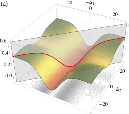
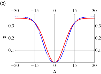
Figure 1: (Color online) Three-photon coincidence rate $\wp(\mathbf{\Delta},\Omega)$ for a three- photon passive optical interferometer with one photon entering each input port shown. The rate is shown as (a) a surface plot, with the solid (red) line corresponding to $(\Delta,-\Delta)$ for photons 1 and 3 arriving at the same time, and (b) the $(\Delta,-\Delta)$ and $(\Delta,\Delta)$ lines as the solid (red) and dashed (blue) loci, respectively. Here $\Omega=(\pi/3,0,\pi/5,\pi/2,\pi/3,\pi/4,0,0)$, and the single-photon spectral widths are identically $\sigma_{0}=0.1$.

We can clearly see from Fig. 1(b) that the backgrounds given at $\Delta\to\infty$ of the diagonal and antidiagonal lines are different. The diagonal is given by a Gaussian, whereas the antidiagonal is a linear combination of Gaussians. Of course at $\tau=0$ both the diagonal and the antidiagonal collapses to a single value and that is the modulus square of the permanent.

V Conclusions

We have developed a theory and a formalism for studying three-photon coincidence rates at the output of a three-channel passive optical interferometer. The input is three photons, one of which enters each of the three input ports of the interferometer. The photons are in pulse modes in order to ensure that controllable delays can be applied to each photon independently. Other than the delay times, the photons are treated as identical in every way. The three-photon coincidence rate is calculated by using integrals over frequency modes and exploiting permutation groups, SU(3) Lie group theory, representation theory, and the theory of immanants, which includes determinants and permanents of matrices as special cases.

The analysis we present here builds on our earlier brief study of non-simultaneous identical photons and their coincidences in passive three-channel optical interferometry, but here we elaborate on the many technical aspects and study asymptotic behavior, which helps us to characterize and understand the photon-coincidence-rate landscape. Furthermore, we employ here a distinct description of the photon counters: in contrast to our earlier work, which employed an idealistic dualism between source photons and photon detection, here we discuss the coincidence-rate landscape in terms of the measurement operator corresponding to currently used detectors.

A key contribution of our work is as a generalization of the Hong-Ou-Mandel dip, which is one of the most important demonstrations and tools used in quantum optics. The Hong-Ou-Mandel dip phenomenon hinges on the observation that identical photons entering two ports of a balanced beam splitter yield an output corresponding to a superposition of both photons exiting the two ports together in tandem. Experimentally the dip is observed by varying the relative delay time between the arrival of the two photons, thus controlling their mutual degree of distinguishability from indistinguishable where the photon arrivals are simultaneously to completely distinguishable when the photon arrivals are separated by more than the duration of the photon pulses.

We have generalized to controllable distinguishability of the three photons entering a general three-channel passive linear optical interferometer. Although this controllability is desirable for practical reasons, the mathematics used to describe this three-photon generalization of the Hong-Ou-Mandel dip is nontrivial and beautiful in its application of group theory.

Our work shows the path forward to considering more photons entering interferometers with at least as many channels as photons, which is the case of interest for BosonSampling. Whereas the BosonSampling problem is framed in the context of simultaneous photon arrival times, thereby leading to matrix permanents in the sampling computations, our work opens BosonSampling to nonsimultaneity of photons, hence the role of immanants in the sampling of photon coincidence rates. The case of three photons in three modes is the simplest situation where the theory requires immanants beyond the permanent and the determinant.

In summary, our work generalizes the Hong-Ou-Mandel dip to the three-photon, three-channel case and points the way forward to analyze further multi-photon, multichannel generalizations. Our work is important for characterizing and understanding the consequent photon-coincidence landscapes. In addition, our use of group theory to study controllable delays in photon arrival times shows how the BosonSampling device can yield rates that depend on matrix immanants, which generalizes the matrix permanent analysis in the original BosonSampling studies.

Appendix A Essentials concerning $\mathfrak{su}$(3) and SU(3)

The Lie algebra $\mathfrak{su}$(3) is spanned by six ladder operators

$$\hat{C}_{12},\hat{C}_{13},\hat{C}_{23},\hat{C}_{21},\hat{C}_{31},\hat{C}_{32}$$ (102)

and two commuting ‘weight’ operators expressed here as

$$\hat{h}_{1}:=\hat{C}_{11}-\hat{C}_{22},\;\hat{h}_{2}:=\hat{C}_{22}-\hat{C}_{33}.$$ (103)

The operators $\hat{C}_{ij}$ satisfy the commutation relations

$$\left[\hat{C}_{ij},\hat{C}_{k\ell}\right]=\hat{C}_{i\ell}\delta_{jk}-\hat{C}_{kj}\delta_{\ell i}.$$ (104)

Within the context of our work, it is convenient to realize these operators in terms of photon creation and destruction operators as

$$\hat{C}_{ij}=\hat{a}^{\dagger}_{i}(\omega_{1})\hat{a}_{j}(\omega_{1})+\hat{a}^{\dagger}_{i}(\omega_{2})\hat{a}_{j}(\omega_{2})+\hat{a}^{\dagger}_{i}(\omega_{3})\hat{a}_{j}(\omega_{3}).$$ (105)

Note that $\hat{C}_{ij}$ is invariant (unchanged) by permutation of the frequencies. Thus, if a state is constructed to have specific symmetries under permutation of the frequencies, the action of $\hat{C}_{ij}$ maps this state to another having the same specific symmetries under permutation of the frequencies.

Of fundamental importance in representations of $\mathfrak{su}$(3) is the so–called highest-weight state. This is a state annihilated by all the “raising operators”: $\hat{C}_{12},\hat{C}_{13}$, and $\hat{C}_{23}$. For instance, the states

$$\left|\hbox{\small\Yvcentermath 1$\young(12,3)$}\right\rangle= \frac{1}{\sqrt{2}}\Big{(}\hat{a}_{1}^{\dagger}(\omega_{1})\hat{a}_{2}^{\dagger}(\omega_{3})$$

$$-\hat{a}_{2}^{\dagger}(\omega_{1})\hat{a}_{1}^{\dagger}(\omega_{3})\Big{)}\hat{a}_{1}^{\dagger}(\omega_{2})|0\rangle$$ (106)

and

$$\left|\hbox{\small\Yvcentermath 1$\young(13,2)$}\right\rangle= \frac{1}{\sqrt{2}}\Big{(}\hat{a}_{1}^{\dagger}(\omega_{1})\hat{a}_{2}^{\dagger}(\omega_{2})$$

$$-\hat{a}_{2}^{\dagger}(\omega_{1})\hat{a}_{1}^{\dagger}(\omega_{2})\Big{)}\hat{a}_{1}^{\dagger}(\omega_{3})|0\rangle$$ (107)

are both highest-weight states (under the action of the raising operators given in Eq. (105).)

The weight of a state is the vector $(p,q)$ of eigenvalues of the operators $\hat{h}_{1}$ and $\hat{h}_{2}$. In terms of occupation number $(n_{1},n_{2},n_{3})$, the weight of a state is therefore simply $(n_{1}-n_{2},n_{2}-n_{3})$ and is frequency independent.

The two states of Eqs. (A) and (A) both have weight $(1,1)$. Because all the states of a representation can be obtained by repeatedly acting on the highest-weight state using the lowering operators $\hat{C}_{21},\hat{C}_{31}$, and $\hat{C}_{32}$, the weight of the highest weight state is used to label states in the whole representation.

For finite-dimensional unitary representations of $\mathfrak{su}$(3), one can always choose the components $(p,q)$ of the highest-weight to be non-negative integers. The dimensionality of the representation $(p,q)$ is

$$(p+1)(q+1)(p+q+2)/2,$$ (108)

so that dim$[(1,1)]=8$.

The two states of Eqs. (A) and (A) are not orthogonal; however, since a linear combination of those states is also a highest-weight state, it is possible to orthonormalize them using the usual Gram-Schmidt method. For instance,

$$\ket{1} =\left|\hbox{\small\Yvcentermath 1$\young(12,3)$}\right\rangle\,,$$ (109)

$$\ket{2} =\frac{1}{\sqrt{3}}\left|\hbox{\small\Yvcentermath 1$\young(12,3)$}\right\rangle-\frac{2}{\sqrt{3}}\left|\hbox{\small\Yvcentermath 1$\young(13,2)$}\right\rangle.$$ (110)

These can serve as distinct highest-weight states for the two distinct copies of the irrep $(1,1)$ or ${\Yboxdim{6pt}\Yvcentermath 1\yng(2,1)}$ that occur in the decomposition of our Hilbert state. Obviously the choice of $\ket{1}$ and $\ket{2}$ as highest-weight states with weight (1,1) is not unique, but all other highest-weight states with weight (1,1) can be written as a linear combination of $\ket{1}$ and $\ket{2}$; if not, there would be a third copy of (1,1) in the Hilbert space.

The matrix representations of elements of $\mathfrak{su}$(3) obtained using either highest-weight state is equivalent ; i.e., they differ by at most a common unitary change of basis. Nevertheless, any state obtained by lowering operators acting on $\ket{1}$ are always orthogonal to states obtained by lowering operators acting on $\ket{2}$.

Now consider states of the form

$$\ket{(1,1)111;0}_{ijk}= \frac{1}{\sqrt{2}}\Big{(}\hat{a}_{2}^{\dagger}(\omega_{i})\hat{a}_{3}^{\dagger}(\omega_{j})$$

$$-\hat{a}_{2}^{\dagger}(\omega_{j})\hat{a}_{3}^{\dagger}(\omega_{i})\Big{)}\hat{a}_{1}^{\dagger}(\omega_{k})|0\rangle,$$ (111)

for $i\neq j\neq k\neq i$.

The triple $111$ indicates that they are constructed as superpositions of states with one quantum in each mode; the weight of these states is $(0,0)$. They are obviously antisymmetric under permutation of modes 2 and 3, and under permutation of frequencies $\omega_{i}$ and $\omega_{j}$. They are also annihilated by the operators $\hat{C}_{23}$ and $\hat{C}_{32}$; they are eigenstates of $\hat{h}_{2}$ with eigenvalue 0. If we observe that the operators $\{\hat{C}_{23},\hat{C}_{32},\frac{1}{2}\hat{h}_{2}\}$ have the same commutation relations as the angular momentum operators, we conclude that $\ket{(1,1)111;0}_{ijk}$ are in fact states of angular momentum $I_{23}=0$ (i.e., singlet) states. This is the interpretation of the last index $0$ in the states.

States with weight $(0,0)$ and $I=0$ in both ${\Yboxdim{6pt}\Yvcentermath 1\yng(2,1)}$ representations are linear combinations of the $\ket{(1,1)111;0}_{ijk}$ states. For instance, the state

$$\left|(1,1)111;0\right\rangle_{1}= -\frac{\ket{(1,1)111;0}_{231}}{\sqrt{6}}$$

$$-\frac{\sqrt{2}\ket{(1,1)111;0}_{132}}{\sqrt{3}}$$

$$+\frac{\ket{(1,1)111;0}_{213}}{\sqrt{6}}$$ (112)

is in the representation having $\ket{1}$ of Eq. (109) as the highest weight. As a linear combination of states antisymmetric under exchange of modes 2 and 3, $\left|(1,1)111;0\right\rangle_{1}$ is itself antisymmetric under such exchange.

On the other hand, states of the form

$$\ket{(1,1)111;1}_{ijk}= \frac{1}{\sqrt{2}}\Big{(}\hat{a}_{2}^{\dagger}(\omega_{i})\hat{a}_{3}^{\dagger}(\omega_{j})$$

$$+\hat{a}_{2}^{\dagger}(\omega_{j})\hat{a}_{3}^{\dagger}(\omega_{i})\Big{)}\hat{a}_{1}^{\dagger}(\omega_{k})|0\rangle,$$ (113)

where $i\neq j\neq k\neq i$ can be shown to have angular momentum $I_{23}=1$. They are symmetric under permutation of modes 2 and 3 and under permutation of frequencies $\omega_{i}$ and $\omega_{j}$.

States with weight $(0,0)$ and $I=1$ in both ${\Yboxdim{6pt}\Yvcentermath 1\yng(2,1)}$ representations are linear combinations of the $\ket{(1,1)111;1}_{ijk}$ states. For instance, the state

$$|(1,1)111;1\rangle_{1}=\frac{\ket{(1,1)111;1}_{231}}{\sqrt{2}}-\frac{\ket{(1,1)111;1}_{213}}{\sqrt{2}}$$ (114)

is in the representation having $\ket{1}$ of Eq. (109) as the highest weight. As it is constructed from states explicitly symmetric under exchange of modes 2 and 3, $|(1,1)111;1\rangle_{1}$ is itself symmetric under this permutation of modes.

Hence we see a feature of the irrep ${\Yboxdim{6pt}\Yvcentermath 1\yng(2,1)}$ of $\mathfrak{su}$(3) that does not occur in angular momentum theory: it is possible to have distinct states such as $|(1,1)111;0\rangle_{1}$ and $|(1,1)111;1\rangle_{1}$, with the same weight ; i.e. the weight is not enough to uniquely identify the state. [This multiplicity of weight never occurs in $\mathfrak{su}(2)$, where the integral weight $2m$ is enough to completely identify the state in the irrep.] In addition to the weight, one must in general supply an additional index, $I_{23}$. In $\mathfrak{su}$(3) representations of type $(p,0)$ or $(0,q)$ this extra label is not necessary and often not indicated.

The states $|(1,1)111;0\rangle_{ijk}$ and $\ket{(1,1)111;1}_{ijk}$ of Eqs. (A) and (A) are not the only possible states that can be used to construct zero-weight states with desirable permutation symmetries: labeling states with the weight using $I_{23}$ is not the only possible choice. We can consider, for instance,

$$\widetilde{\left|(1,1)111;0\right\rangle}_{ijk}$$

$$=\left(\hat{a}_{1}^{\dagger}(\omega_{i})\hat{a}_{2}^{\dagger}(\omega_{j})-\hat{a}_{2}^{\dagger}(\omega_{j})\hat{a}_{1}^{\dagger}(\omega_{i})\right)\hat{a}_{3}^{\dagger}(\omega_{k})|0\rangle$$ (115)

and

$$\widetilde{\ket{(1,1)111;1}}_{ijk}$$

$$\quad=\left(\hat{a}_{1}^{\dagger}(\omega_{i})\hat{a}_{2}^{\dagger}(\omega_{j})+\hat{a}_{2}^{\dagger}(\omega_{j})\hat{a}_{1}^{\dagger}(\omega_{i})\right)\hat{a}_{3}^{\dagger}(\omega_{k})|0\rangle.$$ (116)

These states are now obviously states of angular momentum $I_{12}=0$ and $I_{12}=1$ respectively, where the angular momentum algebra $\mathfrak{su}(2)_{12}$ is spanned by $\{\hat{C}_{12},\hat{C}_{12},\frac{1}{2}\hat{h}_{1}\}$.

The states (115) and (116) can be used to construct an alternative basis for the weight-$0$ subspace of the irrep with highest weight state $\ket{1}$. In other words states $\widetilde{\ket{(1,1)111;0}}_{1}$ and $\widetilde{\ket{(1,1)111;1}}_{1}$ can be defined such that they carry the angular momentum labels $I_{12}=0$ and $1$ respectively, defined in terms of $\mathfrak{su}(2)_{12}$. These states are appropriate linear combinations of $\widetilde{\ket{(1,1)111;0}}_{ijk}$ or $\widetilde{\ket{(1,1)111;1}}_{ijk}$ states and so antisymmetric (respectively symmetric) under exchange of modes 1 and 2. The group functions defined in terms of basis states like

$$\widetilde{\ket{(1,1)111;0}}_{1}\text{ and }\widetilde{\ket{(1,1)111;1}}_{1}$$

with $I_{12}$ labeling the angular momentum properties of the states are denoted $\tilde{D}^{(p,q)}_{(111)J_{12};(111)I_{12}}$.

Using $\mathfrak{su}(2)_{12}$ to label states represents a change of basis from a previous labeling scheme Rowe et al. (1999), where $\mathfrak{su}(2)_{23}$ is used. Thus, the states in $\mathfrak{su}(2)_{12}$ are linear combinations of those in $\mathfrak{su}(2)_{23}$, so that

$$\tilde{D}^{(p,q)}_{(111)J_{12};(111)I_{12}}$$

are linear combinations of the

$$D^{(p,q)}_{(111)J;(111)I}$$

states used previous Rowe et al. (1999) and in Appendix B. Some explicit examples of transformations, required for our analysis, are given in Eqs. (120) and (121).

Finally, we note that it is also possible, following exactly the same procedure as above, to use the subalgebra $\mathfrak{su}(2)_{13}$ to label states. This procedure corresponds to just another change of basis, and the resulting $D$ functions are denoted $\bar{D}$.

Appendix B Explicit expression of some SU(3) D-functions

Some functions of the $D^{(p,q)}_{(111)J;(111)I}$ type useful in constructing permanents and immanents are listed in Table III.

Table 3: Functions of the $D^{(p,q)}_{(111)J;(111)I}$ type useful in constructing permanents and immanants.

$(p,q)$	Diagram	$(J,I)$	$D^{(p,q)}_{(111)J;(111)I}(\Omega)$
(3,0)	(3)	(1,1)	$\cos\beta_{1}\cos\beta_{2}\cos\beta_{3}$
			$-\frac{1}{4}\sin\beta_{1}\cos\frac{\beta_{2}}{2}\sin\beta_{3}\left(3\text{e}^{i(\alpha_{1}-\alpha_{3})}\cos\beta_{2}-\text{e}^{i(\alpha_{1}-\alpha_{3})}+2\text{e}^{-i(\alpha_{1}-\alpha_{3})}\right)$
(1,1)	1 $\yng(2,1)$	(1,1)	$\frac{1}{4}\left(\cos\beta_{1}\cos\beta_{3}(\cos\beta_{2}+3)-4\cos(\alpha_{1}-\alpha_{3})\,\sin\beta_{1}\cos\frac{\beta_{2}}{2}\sin\beta_{3}\right)$
		(1,0)	$-\frac{1}{2}\sqrt{3}\cos\beta_{1}\sin^{2}\frac{\beta_{2}}{2}$
		(0,1)	$-\frac{1}{2}\sqrt{3}\sin^{2}\frac{\beta_{2}}{2}\cos\beta_{3}$
		(0,0)	$\frac{1}{4}(3\cos\beta_{2}+1)$

The functions

$$\tilde{D}^{\Yboxdim{4pt}\Yvcentermath 1\yng(2,1)}_{(111)J_{12};(111)I_{12}},$$

with $I_{12}$ a good quantum number, are related by a linear transformation to the functions

$$D^{\Yboxdim{4pt}\Yvcentermath 1\yng(2,1)}_{(111)J_{23};(111)I_{23}},$$

with $I_{23}$ a good quantum number. Explicitly, using the notation of  Rowe et al. (1999), the states in the $I_{12}$ basis are defined by

$$|(1,1)111;I_{12}\rangle:=\left[\psi_{\nu_{3}}(3)\otimes\left[\psi_{\nu_{1}}(1)\otimes\psi_{\nu_{2}}(2)\right]^{I_{12}}\right]^{1/2}_{1/2}$$ (117)

and can be expanded in terms of the $I_{23}$ states so that

$$|(1,1)111;I_{12}=0\rangle= -\frac{1}{2}|(1,1)111;I_{23}=0\rangle+\frac{\sqrt{3}}{2}|(1,1)111;I_{23}=1\rangle\,,$$ (118)

$$|(1,1)111;I_{12}=1\rangle= -\frac{\sqrt{3}}{2}|(1,1)111;I_{23}=0\rangle-\frac{1}{2}|(1,1)111;I_{23}=1\rangle.$$ (119)

Therefore,

$$\tilde{D}^{\Yboxdim{4pt}\Yvcentermath 1\yng(2,1)}_{(111)0;(111)1}= \frac{\sqrt{3}}{4}D^{\Yboxdim{4pt}\Yvcentermath 1\yng(2,1)}_{(111)0;(111)0}-\frac{\sqrt{3}}{4}D^{\Yboxdim{4pt}\Yvcentermath 1\yng(2,1)}_{(111)1;(111)1}-\frac{3}{4}D^{\Yboxdim{4pt}\Yvcentermath 1\yng(2,1)}_{(111)1;(111)0}+\frac{1}{4}D^{\Yboxdim{4pt}\Yvcentermath 1\yng(2,1)}_{(111)0;(111)1},$$ (120)

$$\tilde{D}^{\Yboxdim{4pt}\Yvcentermath 1\yng(2,1)}_{(111)1;(111)1}= \frac{3}{4}D^{\Yboxdim{4pt}\Yvcentermath 1\yng(2,1)}_{(111)0;(111)0}+\frac{\sqrt{3}}{4}D^{\Yboxdim{4pt}\Yvcentermath 1\yng(2,1)}_{(111)0;(111)1}+\frac{\sqrt{3}}{4}D^{\Yboxdim{4pt}\Yvcentermath 1\yng(2,1)}_{(111)1;(111)0}+\frac{1}{4}D^{\Yboxdim{4pt}\Yvcentermath 1\yng(2,1)}_{(111)1;(111)1}.$$ (121)

and

$$\tilde{D}^{\Yboxdim{4pt}\Yvcentermath 1\yng(3)}_{(111)1;(111)1}=D^{\Yboxdim{4pt}\Yvcentermath 1\yng(3)}_{(111)1;(111)1}.$$ (122)

As discussed in the text and Appendix A, these functions are useful when analyzing the symmetry properties of states under permutations of modes 1 and 2.

Appendix C Explicit expression of rates

In order to obtain a general expression for the rate, we need first to expand the square of the modulus of Eq. (78) and then integrate. The resultant expression thus contains sums of products of the type

$$(a_{ijk})^{*}(a_{i^{\prime}j^{\prime}k^{\prime}})M_{ijk,i^{\prime}j^{\prime}k^{\prime}},$$

where $M_{ijk,i^{\prime}j^{\prime}k^{\prime}}$ is a factor obtained by integration of the frequencies in the term containing $(a_{ijk})^{*}(a_{i^{\prime}j^{\prime}k^{\prime}})$. These $M_{ijk,i^{\prime}j^{\prime}k^{\prime}}$ factors can be collected in a matrix with column labeled by $a_{ijk}$ and rows labeled by $(a_{ijk})^{*}$.

Upon integration, Eq. (78) for the three-photon coincidence rate is written explicitly in terms of the time-of-arrival vector $\bm{\tau}$ of the photons in mode 1, 2, and 3 respectively. For $\bm{\tau}$ and $\bm{\Delta}$ related by expression (3), this rate is given by

$$\wp(\bm{\Delta};\Omega)= \bm{a}(\Omega)^{\dagger}M_{\text{rate}}(\bm{\tau})\bm{a}(\Omega).$$ (123)

Here $M_{\text{rate}}$ is the $6\times 6$ symmetric matrix

$$M_{\text{rate}}=\begin{pmatrix}1&\text{e}^{-\sigma^{2}(\tau_{2}-\tau_{3})^{2}}&\text{e}^{-\sigma^{2}(\tau_{1}-\tau_{2})^{2}}&\text{e}^{-\sigma^{2}\tau_{C}^{2}}&\text{e}^{-\sigma^{2}\tau_{C}^{2}}&\text{e}^{-\sigma^{2}(\tau_{1}-\tau_{3})^{2}}\\ \text{e}^{-\sigma^{2}(\tau_{2}-\tau_{3})^{2}}&1&\text{e}^{-\sigma^{2}\tau_{C}^{2}}&\text{e}^{-\sigma^{2}(\tau_{1}-\tau_{3})^{2}}&\text{e}^{-\sigma^{2}(\tau_{1}-\tau_{2})^{2}}&\text{e}^{-\sigma^{2}\tau_{C}^{2}}\\ \text{e}^{-\sigma^{2}(\tau_{1}-\tau_{2})^{2}}&\text{e}^{-\sigma^{2}\tau_{C}^{2}}&1&\text{e}^{-\sigma^{2}(\tau_{2}-\tau_{3})^{2}}&\text{e}^{-\sigma^{2}(\tau_{1}-\tau_{3})^{2}}&\text{e}^{-\sigma^{2}\tau_{C}^{2}}\\ \text{e}^{-\sigma^{2}\tau_{C}^{2}}&\text{e}^{-\sigma^{2}(\tau_{1}-\tau_{3})^{2}}&\text{e}^{-\sigma^{2}(\tau_{2}-\tau_{3})^{2}}&1&\text{e}^{-\sigma^{2}\tau_{C}^{2}}&\text{e}^{-\sigma^{2}(\tau_{1}^{2}-\tau_{2})^{2}}\\ \text{e}^{-\sigma^{2}\tau_{C}^{2}}&\text{e}^{-\sigma^{2}(\tau_{1}-\tau_{2})^{2}}&\text{e}^{-\sigma^{2}(\tau_{1}-\tau_{3})^{2}}&\text{e}^{-\sigma^{2}\tau_{C}^{2}}&1&\text{e}^{-\sigma^{2}(\tau_{2}-\tau_{3})^{2}}\\ \text{e}^{-\sigma^{2}(\tau_{1}-\tau_{3})^{2}}&\text{e}^{-\sigma^{2}\tau_{C}^{2}}&\text{e}^{-\sigma^{2}\tau_{C}^{2}}&\text{e}^{-\sigma^{2}(\tau_{1}-\tau_{2})^{2}}&\text{e}^{-\sigma^{2}(\tau_{2}-\tau_{3})^{2}}&1\end{pmatrix}$$ (124)

with

$$\tau_{C}=\sqrt{|\bm{\tau}|^{2}-\tau_{2}\tau_{3}-\tau_{1}\tau_{2}-\tau_{1}\tau_{3}}$$ (125)

and

$$\bm{a}(\Omega)=\begin{pmatrix}a_{123}(\Omega)\\ a_{132}(\Omega)\\ a_{213}(\Omega)\\ a_{231}(\Omega)\\ a_{312}(\Omega)\\ a_{321}(\Omega)\end{pmatrix}.$$ (126)

for which $\{a_{ijk}\}$ is defined in Eq. (53).

References

• Hong et al. (1987) C. K. Hong, Z. Y. Ou,  and L. Mandel, Phys. Rev. Lett. 59, 2044 (1987).
• Campos (2000) R. A. Campos, Phys. Rev. A 62, 013809 (2000).
• Knill et al. (2001) E. Knill, R. Laflamme,  and G. J. Milburn, Nature 409, 46 (2001).
• Berry et al. (2004a) D. W. Berry, S. Scheel, B. C. Sanders,  and P. L. Knight, Phys. Rev. A 69, 031806 (2004a).
• Berry et al. (2004b) D. W. Berry, S. Scheel, C. R. Myers, B. C. Sanders, P. L. Knight,  and R. Laflamme, New J. Phys. 6, 93 (2004b).
• Berry et al. (2006) D. W. Berry, A. I. Lvovsky,  and B. C. Sanders, Opt. Lett. 31, 107 (2006).
• Broome et al. (2010) M. A. Broome, A. Fedrizzi, B. P. Lanyon, I. Kassal, A. Aspuru-Guzik,  and A. G. White, Phys. Rev. Lett. 104, 153602 (2010).
• Schreiber et al. (2011) A. Schreiber, K. N. Cassemiro, V. Potoček, A. Gábris, I. Jex,  and C. Silberhorn, Phys. Rev. Lett. 106, 180403 (2011).
• Schreiber et al. (2012) A. Schreiber, A. Gábris, P. P. Rohde, K. Laiho, M. S̆tefan̆ák, V. Potoc̆ek, C. Hamilton, I. Jex,  and C. Silberhorn, Science 336, 55 (2012)http://www.sciencemag.org/content/336/6077/55.full.pdf .
• Sansoni et al. (2012) L. Sansoni, F. Sciarrino, G. Vallone, P. Mataloni, A. Crespi, R. Ramponi,  and R. Osellame, Phys. Rev. Lett. 108, 010502 (2012).
• Aaronson and Arkhipov (2011) S. Aaronson and A. Arkhipov, in Proc. 43rd Ann. ACM Symp. Theory Comp., STOC ’11 (2011).
• Metcalf et al. (2013) B. J. Metcalf, N. Thomas-Peter, J. B. Spring, D. Kundys, M. A. Broome, P. C. Humphreys, X.-M. Jin, M. Barbieri, W. S. Kolthammer, J. C. Gates, B. J. Smith, N. K. Langford, P. G. R. Smith,  and I. A. Walmsley, Nat. Commun. 4, 1356 (2013).
• Broome et al. (2013) M. A. Broome, A. Fedrizzi, S. Rahimi-Keshari, J. Dove, S. Aaronson, T. C. Ralph,  and A. G. White, Science 339, 794 (2013).
• Spring et al. (2013) J. B. Spring, B. J. Metcalf, P. C. Humphreys, W. S. Kolthammer, X.-M. Jin, M. Barbieri, A. Datta, N. Thomas-Peter, N. K. Langford, D. Kundys, J. C. Gates, B. J. Smith, P. G. R. Smith,  and I. A. Walmsley, Science 339, 798 (2013).
• Tillmann et al. (2013) M. Tillmann, B. Dakić, R. Heilmann, S. Nolte, A. Szameit,  and P. Walther, Nat. Phot. 7, 3 (2013).
• Crespi et al. (2013) A. Crespi, R. Osellame, R. Ramponi, D. J. Brod, E. F. Galvao, N. Spagnolo, C. Vitelli, E. Maiorino, P. Mataloni,  and F. Sciarrino, Nat. Phot. 7, 545 (2013).
• (17) P. P. Rohde, K. R. Motes, A. Peruzzo, M. A. Broome, A. G. White,  and W. J. Munro, “Boson-sampling: A new route towards linear optics quantum computing,” Private Communication.
• Spagnolo et al. (2013) N. Spagnolo, C. Vitelli, M. Bentivegna, D. J. Brod, A. Crespi, F. Flamini, S. Giacomini, G. Milani, R. Ramponi, P. Mataloni, R. Osellame, E. F. Galvao,  and F. Sciarrino, “Efficient experimental validation of photonic bosonic sampling against the uniform distribution,”  (2013), arXiv:1311.1622.
• Carolan et al. (2013) J. Carolan, J. D. A. Meinecke, P. Shadbolt, N. J. Russell, N. Ismail, K. Wörhoff, T. Rudolph, M. G. Thompson, J. L. O’Brien, J. C. F. Matthews,  and A. Laing, “On the experimental verification of quantum complexity in linear optics,”  (2013), arXiv:1311.2913.
• Ra et al. (2013) Y.-S. Ra, M. C. Tichy, H.-T. Lim, O. Kwon, F. Mintert, A. Buchleitner,  and Y.-H. Kim, Proceedings of the National Academy of Sciences  (2013), 10.1073/pnas.1206910110.
• Tan et al. (2013) S.-H. Tan, Y. Y. Gao, H. de Guise,  and B. C. Sanders, Phys. Rev. Lett. 110, 113603 (2013).
• Littlewood and Richardson (1934) D. E. Littlewood and A. R. Richardson, Phil. Trans. R. Soc. Lond. A 233, 99 (1934).
• Littlewood (1950) D. E. Littlewood, The Theory of Group Characters and Matrix Representations of Groups, 2nd ed. (Clarendon, Oxford University Press, 1950).
• Valiant (1979) L. Valiant, Theor. Comput. Sci. 8, 189 (1979).
• Bürgisser (2000) P. Bürgisser, SIAM J. Comput. 30, 1023 (2000).
• Rohde and Ralph (2006) P. P. Rohde and T. C. Ralph, Journal of Modern Optics 53, 1589 (2006).
• Bouland and Aaronson (2014) A. Bouland and S. Aaronson, Phys. Rev. A 89, 062316 (2014).
• Campos et al. (1989) R. A. Campos, B. E. A. Saleh,  and M. C. Teich, Phys. Rev. A 40, 1371 (1989).
• Varshalovich et al. (1988) D. A. Varshalovich, A. N. Moskalev,  and V. K. Khersonskii, Quantum Theory of Angular Momentum (World Scientific, Singapore, 1988).
• Wybourne (1970) B. G. Wybourne, Symmetry Principle and Atomic Spectroscopy, 1st ed. (Wiley, New York, 1970).
• Tung (1985) W.-K. Tung, Group Theory in Physics (World Scientific, Singapore, 1985).
• Fulton and Harris (1991) W. Fulton and J. Harris, Representation Theory (Springer, New York, 1991).
• Yong (2007) A. Yong, Notices of the AMS 54, 240 (2007).
• Weyl (1939) H. Weyl, The Classical Groups. Their Invariants and Representations (Princeton University Press, Princeton, 1939).
• Lichtenberg (1978) D. B. Lichtenberg, Unitary Symmetry and Elementary Particles, 2nd ed. (Academic, New York, 1978).
• Rowe and Wood (2010) D. J. Rowe and J. L. Wood, Fundamentals of Nuclear Models (World Scientific, 2010).
• Bartlett and Sanders (2002) S. D. Bartlett and B. C. Sanders, Phys. Rev. A 65, 042304 (2002).
• Baird and Biedenharn (1963) G. E. Baird and L. C. Biedenharn, J. Math. Phys. 4, 1449 (1963).
• Slansky (1981) R. Slansky, Phys. Rep. 79, 1 (1981).
• Rowe et al. (1999) D. J. Rowe, B. C. Sanders,  and H. de Guise, J. Math. Phys. 40, 3604 (1999).
• Klimov and de Guise (2010) A. B. Klimov and H. de Guise, J, Phys. A 43, 402001 (2010).
• Yurke et al. (1986) B. Yurke, S. L. McCall,  and J. R. Klauder, Phys. Rev. A 33, 4033 (1986).
• Speiser (1963) D. Speiser, Lectures of the Istanbul Summer School of Theoretical Physics, Vol. 1 (Gordon and Breach, New York, 1963).
• O’Reilly (1982) M. F. O’Reilly, J. Math. Phys. 23, 2022 (1982).
• Dresselhaus et al. (2007) M. S. Dresselhaus, G. Dresselhaus,  and A. Jorio, Group theory (Springer, Berlin, 2007).
• Lazard (1983) D. Lazard, “Computer algebra,”  (Springer, Berlin, 1983) Chap. Gröbner bases, Gaussian elimination and resolution of systems of algebraic equations, pp. 146–156.