Single-Photon Storing in Coupled Non-Markovian Atom-Cavity System

Abstract

Taking the non-Markovian effect into account, we study how to store a single photon of arbitrary temporal shape in a single atom coupled to an optical cavity. Our model applies to Raman transitions in three-level atoms with one branch of the transition controlled by a driving pulse, and the other coupled to the cavity. For any couplings of input field to the optical cavity and detunings of the atom from the driving pulse and cavity, we extend the input-output relation from Markovian dynamics to non-Markovian one. For most possible photon shapes, we derive an analytic expression for the driving pulse in order to completely map the input photon into the atom. We find that, the amplitude of the driving pulse depends only on the detuning of the atom from the frequency of the cavity, i.e., the detuning of the atom to the driving pulse has no effect on the strength of the driving pulse.

I Introduction

Quantum networks composed of local nodes and quantum channels have attracted much attention in recent years due to a wide range of possible applications in quantum information science DiVincenzo1998393 ; Knill2001409 ; Cirac199959 ; DiVincenzo200048 ; Cirac199778 ; Duan200367 ; Liu201059 , for example, quantum communication and distributed quantum computing. An important class of schemes for quantum communication and computing is based on an elementary process in which single quanta of excitation are transferred back and forth between an atom and a photonOxborrow200546 . This is achieved within the framework of cavity electrodynamics, which is also the most promising candidate for deterministically producing streams of single photons Law199744 ; Kuhn199969 ; Kuhn200289 ; Sun200469 ; McKwwver2004303 ; Keller2004431 of narrowband and indistinguishable radiation modesLegero200493 .

Dissipative dynamics of cavity-atom system has been well investigated and deeply understood under the Markovian approximationCarmichael1993 . This approximation is valid when the coupling between system and bath is weak such that the perturbation theory can be applied, meanwhile the validity of the Markovian approximation requires that the characteristic time of the bath is sufficiently shorter than that of the system. However, in practice, the coupling of the system to bath is not weak and the memory effect of the bath can not be neglected. Typical examples include optical fields propagating in cavity arrays or in an optical fiberHartmann20062 ; Pellizzari199779 ; Biswas200674 , trapped ions subjected to artificial colored noiseTurchette200062 ; Myatt2000403 ; Maniscalco200469 , and microcavities interacting with a coupled resonator optical waveguide or photonic crystalsStefanou199857 ; Bayindir200084 ; Xu200062 ; Lin200572 ; Longhi200674 , to mention a few.

Previous studies of state transferring (or mapping) between atom and photon in cavity QED are based on Markovian approximation Yao200595 ; Lukin200084 ; Fleischhauer2000179 ; Dilley201285 ; Hong200776 . However, recent studies have shown that Markovian and non-Markovian quantum processesPiilo2008100 ; Piilo200979 ; Maniscalco200673 ; Bellomo200799 play an important role in many fields of physics, e.g., quantum opticsGardiner2000 ; Scully1997 ; Walls1994 and quantum information scienceNielsen2000 ; Bennett2000404 . This motivates us to explore the storing of single photons of arbitrary temporal shape (or a packet) in coupled atom-cavity systems under the non-Markovian approximation.

For this purpose, we first extend the input-output relation in Ref. Dilley201285 from Markovian system to non-Markovian systemZhang201387 . Then we show the difference between Markovian and non-Markovian approximations in the single photon storing. Next we study state transfer from an input photon state to a single-photon cavity dark state by adiabatically evolving the system in the non-Markovian regime, the result is compared with that given by the earlier scheme, we find that these methods are in good agreement with each other.

The remainder of the paper is organized as follows. In Sec. II, we introduce a model to describe the atom-cavity system coupled to input photons and derive the non-Markovian input-output relations, the dynamical equations for the atom-cavity system are also given in this section. In Sec. III, we derive an exact expression for the complex driving pulse with non-zero detunings and non-zero populations of the excited state. In Sec. IV, we study the storing of the single photons taking the non-Markovian processes into account. In Sec. V, we study the adiabatic transfer via dark states between input photon and the cavity-atom system. Discussion and conclusions are given in Sec. VI.

II Equations of motion and non-Markovian input-output relations

We now discuss how to transfer a single-photon state of input field into a single excitation of atom-cavity system. We consider an effective one-dimensional model, which describes a Fabry-Perot cavity coupled to an three-level atom, as shown in Fig. 1. The input and output fields are parallel to the z-axis (perpendicular to the cavity mirrors). The input field partially transmit into the cavity through the mirror at z=0 (the mirror at the right-hand side of the setup), the other mirror of the cavity is assumed to be 100% reflecting.

The input-output field is introduced as a continuum field modeled by a set of oscillators denoted by annihilation operator $\hat{b}(\omega)$, which are coupled to the cavity mode with coupling constants $\kappa(\omega)$. The interaction between the cavity field $\hat{a}$ and the continuum $\hat{b}(\omega)$ is described by the following HamiltonianWalls1994 ; Gardiner198531 ; Fleischhauer2000179 ,

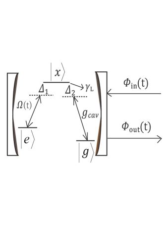
Figure 1: (Color online) Schematic illustration of our system. It consists of a cavity, a three-level atom, and input-output fields. The atom is driven by both the cavity field with coupling constant ${g_{cav}}$ and a classical filed characterized by the driving pulse $\Omega(t)$. The classical and cavity fields are detuning from the atomic resonance by ${\Delta_{1}}$ and ${\Delta_{2}}$, respectively.

$${H_{{\mathop{\rm int}}}}=i\int_{-\infty}^{\infty}{d\omega[\kappa(\omega)\hat{a}{{\hat{b}}^{\dagger}}(\omega)-H.c.}],$$ (1)

where $\left[{b(\omega),{b^{\dagger}}(\omega^{\prime})}\right]=\delta(\omega-\omega^{\prime})$ and $\left[{a,{a^{\dagger}}}\right]=1$. We consider an input field in a general single-photon state $\left|{{\psi_{in}}(t)}\right\rangle=\int{d\omega C_{\omega}^{in}(t){{\hat{b}}^{\dagger}}(\omega)\left|0\right\rangle}$ with $C_{\omega}^{in}(t)=C_{\omega}^{in}({t_{0}}){e^{-i\omega(t-{t_{0}})}}$. Here, $\left|0\right\rangle$ denotes the vacuum state of the continuum $b(\omega)$. In what follows we characterize these fields by an envelope wave function ${\Phi_{in}}(z,t)$ defined by

$${\Phi_{in}}(z,t) = \int d\omega\langle{0_{\omega}}|\hat{b}(\omega){e^{ikz}}\left|{{\psi_{in}}(t)}\right\rangle$$ (2)

$$= \int{d\omega C_{\omega}^{in}(t){e^{ikz}}.}$$

The normalization condition $\int{d\omega{{\left|{C_{\omega}^{in}(t)}\right|}^{2}}}=1$ of the Fourier coefficients implies the normalization of the input wave-function according to Parseval theorem,

$$\int{dt{{\left|{{\Phi_{in}}(z,t)}\right|}^{2}}}=1.$$ (3)

Clearly, $\Phi_{in}(z,t)$ describes a single photon propagating along the z-axis.

To derive an input-output relation for a general non- Markovian quantum system, we write the total Hamiltonian in a rotation frame with respect to the center frequency ${\omega_{c}}$ of the cavity field,

$$H={H_{S}}+{H_{B}}+{H_{{\mathop{\rm int}}}},$$ (4)

with

$${H_{S}}= (\Omega(t){e^{i{\Delta_{1}}t}}{\sigma_{xe}}+{g_{cav}}{\sigma_{xg}}\hat{a}{e^{i{\Delta_{2}}t}}+H.c.)-i{\gamma_{L}}{\sigma_{xx}},$$ (5)

$${H_{B}}= \int_{-\infty}^{\infty}{d\omega{\Omega_{\omega}}{{\hat{b}}^{\dagger}}(\omega)\hat{b}(\omega)},$$

where ${\sigma_{\mu\nu}}=\left|\mu\right\rangle\left\langle\nu\right|(\mu,\nu=x,e,g)$ are the atomic transition operators, and H.c. stands for Hermitian conjugate. $\left|g\right\rangle$ denotes the ground state with energy ${\omega_{g}}=0$ ($\hbar=1$, hereafter), and $\left|e\right\rangle$ denotes the excited state with energy ${\omega_{e}}$. ${\hat{a}}$ is the annihilation operator of the cavity mode with center frequency ${\omega_{c}}$. $\left|e\right\rangle$ to $\left|x\right\rangle$ (with energy ${\omega_{x}}$) transition is driven by the classical field $\Omega(t)$ with frequency ${\nu_{\Omega}}$, the transition from $\left|g\right\rangle$ to $\left|x\right\rangle$ is driven by the cavity mode with coupling constant ${g_{cav}}$. Detuning ${\Delta_{1}}$ is defined as ${\Delta_{1}}={\omega_{x}}-{\omega_{e}}-{\nu_{\Omega}}\equiv{\omega_{xe}}-{\nu_{\Omega}}$, and ${\Delta_{2}}={\omega_{x}}-{\omega_{g}}-{\omega_{c}}\equiv{\omega_{xg}}-{\omega_{c}}$. ${\gamma_{L}}$ denotes the atomic spontaneous emission rate and ${\Omega_{\omega}}=\omega-{\omega_{c}}$ the detuning of the $\omega$-mode from the center frequency of the cavity.

Assuming there is only one photon initially in the input field and the cavity-atom system is not excited, we can restrict the solution and discussion of the total system (4) to the subspace containing zero and a single excitation. This allows us to expand the state vector of the total system at a later time $t$ as,

$$\left|{\psi(t)}\right\rangle= G(t)\left|{g,1,0}\right\rangle+E(t)\left|{e,0,0}\right\rangle+X(t)\left|{x,0,0}\right\rangle$$ (6)

$$+\int_{-\infty}^{\infty}{d\omega{C_{\omega}}(t){{\hat{b}}^{\dagger}}(\omega)\left|{g,0,0}\right\rangle},$$

where $\left|{g,1,0}\right\rangle$ denotes a state with the atom in the ground state $\left|g\right\rangle$, the cavity having a single photon and no photons in the input. $G(t)$ denotes the probability amplitude of the total system being in $\left|{g,1,0}\right\rangle.$ The other states have similar notations. To calculate the probability amplitudes $G(t),E(t),X(t),$ and ${{C_{\omega}}}(t)$, we substitute $\left|{\psi(t)}\right\rangle$ into the Schrödinger equation $i{\partial_{t}}\left|{\psi(t)}\right\rangle=H\left|{\psi(t)}\right\rangle$. Simple calculation yields,

$$\dot{G}= -i{g_{cav}}X{e^{-i{\Delta_{2}}t}}-\int_{-\infty}^{\infty}{d\omega{\kappa^{*}}(\omega){C_{\omega}}},$$ (7)

$$\dot{E}= -i{\Omega^{*}}(t){e^{-i{\Delta_{1}}t}}X,$$

$$\dot{X}= -i\Omega(t){e^{i{\Delta_{1}}t}}E-i{g_{cav}}G{e^{i{\Delta_{2}}t}}-{\gamma_{L}}X,$$

$${{\dot{C}}_{\omega}}= -i{\Omega_{\omega}}{C_{\omega}}+\kappa(\omega)G.$$

Formally integrating the fourth equation of Eq. (7), we obtain

$${{C_{\omega}}(t){\rm{=}}{e^{-i{\Omega_{\omega}}(t-{t_{0}})}}{C_{\omega}}({t_{0}})+\kappa(\omega)\int_{{t_{0}}}^{t}{d\tau G(\tau){e^{-i{\Omega_{\omega}}(t-\tau)}}},}$$ (8)

where ${C_{\omega}}({t_{0}})$ is the initial condition of ${C_{\omega}}(t)$. Similarly,

$${{C_{\omega}}(t){\rm{=}}{e^{-i{\Omega_{\omega}}(t-{t_{1}})}}{C_{\omega}}({t_{1}})-\kappa(\omega)\int_{t}^{{t_{1}}}{d\tau G(\tau){e^{-i{\Omega_{\omega}}(t-\tau)}}},}$$ (9)

where ${t_{1}}\geq t$. The single photon input and output fields ${\Phi_{in}}(0,t)$ and ${\Phi_{out}}(0,t)$ (for simplicity, hereafter we write ${\Phi_{out}}(0,t)$ as ${\Phi_{out}}(t)$, the same notation for ${\Phi_{in}}(t)$) are defined as the Fourier transformation of ${C_{\omega}}({t_{0}})$ and ${C_{\omega}}({t_{1}})$ at $z=0$, respectively.

$${\Phi_{in}}(t)= \frac{{-1}}{{\sqrt{2\pi}}}\int_{-\infty}^{\infty}{d\omega{C_{\omega}}({t_{0}}){e^{-i{\Omega_{\omega}}(t-{t_{0}})}}},$$ (10)

$${\Phi_{out}}(t)= \frac{1}{{\sqrt{2\pi}}}\int_{-\infty}^{\infty}{d\omega{C_{\omega}}({t_{1}}){e^{-i{\Omega_{\omega}}(t-{t_{1}})}}}.$$

Integrating Eq. (8) and Eq. (9) and using Eq. (10), we obtain a non-Markovian input-output relation (change ${t_{1}}\to t$),

$${\Phi_{in}}(t)+{\Phi_{out}}(t)=\int_{{t_{0}}}^{t}{d\tau h(t-\tau)G(\tau)},$$ (11)

where

$$h(t)=\frac{1}{{\sqrt{2\pi}}}\int_{-\infty}^{\infty}{d\omega{e^{-i{\Omega_{\omega}}t}}\kappa(\omega)},$$ (12)

defines the impulse response function that equals the Fourier transform of the coupling strength ${\kappa(\omega)}$. Substituting Eq. (8) into the first equation of Eq. (7), we obtain finally the general equations of motion for the total system,

$$\dot{G}= -i{g_{cav}}X{e^{-i{\Delta_{2}}t}}+N(t)-\int_{0}^{t}{d\tau f(t-\tau)G(\tau)},$$ (13)

$$\dot{E}= -i{\Omega^{*}}(t){e^{-i{\Delta_{1}}t}}X,$$

$$\dot{X}= -i\Omega(t){e^{i{\Delta_{1}}t}}E-i{g_{cav}}G{e^{i{\Delta_{2}}t}}-{\gamma_{L}}X,$$

$${\Phi_{in}}( t)+{\Phi_{out}}(t)=\int_{{t_{0}}}^{t}{d\tau h(t-\tau)G(\tau)},$$

where

$$N(t)=\int_{-\infty}^{\infty}{d\tau{h^{*}}(\tau-t){\Phi_{in}}(\tau)},$$ (14)

is the driving field and

$$f(t-\tau)= \int_{-\infty}^{\infty}{d\zeta{h^{*}}(\tau-\zeta)h(t-\zeta)}$$ (15)

$$= \int_{-\infty}^{\infty}{d\omega{{\left|{\kappa(\omega)}\right|}^{2}}{e^{-i{\Omega_{\omega}}(t-\tau)}}}$$

$$\equiv \int_{-\infty}^{\infty}{d\omega J(\omega){e^{-i{\Omega_{\omega}}(t-\tau)}}},$$

is the memory function of the system, and $J(\omega)=|\kappa(\omega){{\rm{|}}^{2}}$. From the derivation, we find that $h(t)$ and $f(t)$ plays essential roles in the photon storing. Different $h(t)$ and $f(t)$ leads to different non-Markovianity of the dynamics, hence they affect the design of the driving pulse to store a photon into the atom-cavity system.

III driving pulse and excited state population

In this section we present an analytical expression for the driving pulse to completely store an arbitrary photon wave packet ${\Phi_{in}}(t)$ in the atom-cavity system. Obviously completely impedance matching is a necessary condition for this purpose, i.e.,

$${\Phi_{out}}(t)=0,$$ (16)

must be satisfied at any time.

The spectral response function ${\kappa(\omega)}$ for the Fabry-Perot (FP) cavity can be defined by

$$\kappa(\omega)=\sqrt{\frac{\Gamma}{{2\pi}}}\frac{W}{{W-i(\omega-{\omega_{c}})}},$$ (17)

where $\Gamma$ is the cavity-input coupling strength and $W$ is the spectrum bandwidth of the input field. The effective spectral density is then Haikka201081 ; Breuer2002 ; xiong201286

$$J(\omega)=\frac{\Gamma}{{2\pi}}\frac{{{W^{2}}}}{{{W^{2}}+{{(\omega-{\omega_{c}})}^{2}}}}.$$ (18)

In the wide-band limit (i.e., $W\to\infty$), the spectral density approximately takes $J(\omega)\to\frac{\Gamma}{{2\pi}}$, equivalently $\kappa(\omega)\to\sqrt{\frac{\Gamma}{{2\pi}}}$. This describes the case in the Markovian limit. Then according to Eq. (12) and Eq. (15), we have

$$h(t)= \sqrt{\Gamma}\delta(t),$$ (19)

$$f(t)= \Gamma\delta(t).$$

Substituting Eq. (19) into Eq. (13), we obtain the Markovian dynamics of the total systemDilley201285 ; Yao200595 ,

$$\dot{G}= -i{g_{cav}}X{e^{-i{\Delta_{2}}t}}+\sqrt{\Gamma}{\Phi_{in}}(t)-\frac{1}{2}\Gamma G(t),$$ (20)

$$\dot{E}= -i{\Omega^{*}}(t){e^{-i{\Delta_{1}}t}}X,$$

$$\dot{X}= -i\Omega(t){e^{i{\Delta_{1}}t}}E-i{g_{cav}}G{e^{i{\Delta_{2}}t}}-{\gamma_{L}}X,$$

$${\Phi_{in}}( t)+{\Phi_{out}}(t)=\sqrt{\Gamma}G(t).$$

In order to take the non-Markovian effect into account, we calculate the system-field memory function $f(t)$ and the spectral-response function $h(t)$ yu199960 ; Jack199959 ; Breuer2002 by the use of Eq. (17) and Eq. (18), they read,

$${h(t)=W\sqrt{\Gamma}\Theta(t){e^{-Wt}}},$$ (21)

and

$${f(t)=\frac{1}{2}W\Gamma{e^{-W\left|t\right|}}},$$ (22)

where $\Theta(t)$ is the unit step function

$$\Theta(t)=\left\{{\begin{array}[]{*{20}{c}}{1,}&{t\geq 0},\\ {0,}&{t\leq 0}.\end{array}}\right.$$

To store an input photon into the atom-cavity system, it is reasonable to assume that the total system is initially prepared in state ${{{\hat{b}}^{\dagger}}(\omega)\left|{g,0,0}\right\rangle}$, i.e., the initial condition for the equations of motion is,

$$\int{dt{{\left|{{\Phi_{in}}(t)}\right|}^{2}}=1},$$ (24)

$$G(0)=0,$$ (25)

$$X(0)=0,$$ (26)

$$E(0)=0.$$ (27)

Now we calculate the population of the atom in the excited state $\left|{e,0,0}\right\rangle$,

$${\rho_{ee}}(t)= {\rho_{offset}}-{{\tilde{X}}^{2}}(t)$$ (28)

$$+\int_{0}^{t}{dt^{\prime}[2{g_{cav}}\tilde{X}(t^{\prime})G(t^{\prime})-2{\gamma_{L}}{{\tilde{X}}^{2}}(t^{\prime})]}.$$

Eq. (28) shows that the population of excited state ${\rho_{ee}}(t)$ does not depend on the detunings ${\Delta_{1}}$ and ${\Delta_{2}}$. From the derivation below for the complex driving pulse $\Omega(t)$, we see that we should introduce an offset term ${\rho_{offset}}$ phenomenologically to account for the imperfect state preparation–a small initial population in the excited state $\left|e,0,0\right\rangle$. We give the details of the derivations of Eq. (28) in Appendix A.

We can now proceed to derive the complex driving pulse $\Omega(t)$ for completely storing an photon in arbitrary temporal shape with nonzero detunings ${{\Delta_{1}}}$ and ${{\Delta_{2}}}$,

$$\Omega(t)=\alpha(t)+i\beta(t),$$ (29)

where

$$\alpha(t)=[{\partial_{t}}\tilde{X}(t)\cos A(t)-{g_{cav}}G(t)\cos A(t)$$ (30)

$$+{\gamma_{L}}\tilde{X}(t)\cos A(t)+{\Delta_{2}}\tilde{X}(t)\sin A(t)]/\sqrt{{\rho_{ee}}(t)},$$

$$\beta(t)=[{\Delta_{2}}\tilde{X}(t)\cos A(t)-{\partial_{t}}\tilde{X}(t)\sin A(t)$$

$$+{g_{cav}}G(t)\sin A(t)-{\gamma_{L}}\tilde{X}(t)\sin A(t)]/\sqrt{{\rho_{ee}}(t)},$$

with

$$A(t)=-\Delta\cdot t+{\Delta_{2}}\int_{0}^{t}{dt^{\prime}\frac{{{{\tilde{X}}^{2}}(t^{\prime})}}{{{\rho_{ee}}(t^{\prime})}}}.$$ (31)

The details of the derivation of Eq. (29) can also be found in Appendix A.

Modulus and argument of the complex driving pulse $\Omega(t)=\left|{\Omega(t)}\right|{e^{i\theta(t)}}$ is

$$\left|{\Omega(t)}\right|= \sqrt{{\alpha^{2}}(t)+{\beta^{2}}(t)}$$ (32)

$$= \sqrt{\frac{{{{[{\partial_{t}}\tilde{X}(t)-{g_{cav}}G(t)+{\gamma_{L}}\tilde{X}(t)]}^{2}}+{\Delta_{2}}^{2}\tilde{X}{{(t)}^{2}}}}{{{\rho_{ee}}(t)}}},$$ (33)

$$\theta(t)=\arctan\left[{\frac{{\beta(t)}}{{\alpha(t)}}}\right],$$ (34)

which is an analytical expression that defines the complex driving pulse necessary to store completely the desired photon packet. This equation tells us that the modulus of the driving pulse $\Omega(t)$ depends only on the detuning ${{\Delta_{2}}}$, not on the detuning ${{\Delta_{1}}}$.

Under the Markovian approximation (we denote Markovian case by introducing the subscript f) and defining ${X_{f}}(t)=-i{e^{i{\Delta_{2}}t}}{\tilde{X}_{f}}(t)$ and ${E_{f}}(t)={e^{-i{\Delta_{1}}t+i{\Delta_{2}}t}}{\tilde{E}_{f}}(t)$, we obtain from Eq. (20) the following results with nonzero ${\Delta_{1}}$ and ${\Delta_{2}}$

$${G_{f}}(t)= {\Phi_{in}}(t)/\sqrt{\Gamma},$$ (35)

$${{\tilde{X}}_{f}}(t)= [-{{\dot{G}}_{f}}(t)+\frac{1}{2}\Gamma{G_{f}}(t)]/{g_{cav}},$$

$${\rho_{fee}}= {\rho_{offset}}-{{\tilde{X}}_{f}}^{2}$$

$$+\int_{0}^{t}{dt^{\prime}[2{g_{cav}}{{\tilde{X}}_{f}}(t^{\prime}){G_{f}}(t^{\prime})-2{\gamma_{L}}{{\tilde{X}}_{f}}^{2}(t^{\prime})]},$$

$${\Omega_{f}}(t)= {\alpha_{f}}(t)+i{\beta_{f}}(t),$$

where,

$${\alpha_{f}}(t)= [\cos({A_{f}}){\partial_{t}}{{\tilde{X}}_{f}}-{g_{cav}}\cos({A_{f}}){G_{f}}$$ (36)

$$+{\gamma_{L}}\cos({A_{f}}){{\tilde{X}}_{f}}+{\Delta_{2}}\sin({A_{f}}){{\tilde{X}}_{f}}]/\sqrt{{\rho_{fee}}},$$

$${\beta_{f}}(t)= [{\Delta_{2}}\cos({A_{f}}){{\tilde{X}}_{f}}-\sin({A_{f}}){\partial_{t}}{{\tilde{X}}_{f}}$$

$$+{g_{cav}}\sin({A_{f}}){G_{f}}-{\gamma_{L}}\sin({A_{f}}){{\tilde{X}}_{f}}]/\sqrt{{\rho_{fee}}},$$

$${A_{f}}(t)= -\Delta\cdot t+{\Delta_{2}}\int_{0}^{t}{dt^{\prime}\frac{{\tilde{X}_{f}^{2}(t^{\prime})}}{{{\rho_{fee}}(t^{\prime})}}}.$$

Within the Markovian approximation, modulus $\left|{{\Omega_{f}}(t)}\right|$ and argument ${\theta_{f}}(t)$ of the complex driving pulse ${{\Omega_{f}}(t)}$ are formally the same as Eq. (32) and Eq. (34) with the subscript $f$, i.e., $\alpha(t)\to{\alpha_{f}}(t)$ and $\beta(t)\to{\beta_{f}}(t)$. This driving pulse representing the coupling constant between the atom and the driving fields is complex when the detunings are not zero, which is not discussed in the earlier studies.

IV single photons storing and impedance matching

We now consider an realistic input photon packet that starts from time ${t_{0}}$ and ends at time ${t_{e}}$. We assume the packet starts off smoothly, i.e., ${\Phi_{in}}({t_{0}})={\partial_{t}}{\Phi_{in}}({t_{0}})=0$ as described in Vasilev201012 . The second time derivative of the input $\Phi_{in}(t_{0})$ might be nonzero at ${t_{0}}$, thus ${\rm{G(0)}}=0$ in Eq. (54) but

$$\dot{G}({t_{0}})=\frac{{{{\ddot{\Phi}}_{in}}({t_{0}})}}{{W\sqrt{\Gamma}}}\neq 0.$$ (37)

Furthermore, from Eq. (55) together with Eq. (26) and Eq. (25), we find

$$\dot{G}(0)=N(0),$$ (38)

this is the so-called equilibrium condition.

By Eq. (14) and Eq. (21), we can establish a relation between $W$ and $\Gamma$ for arbitrary input photon wave packets ${\Phi_{in}}$

$$\Gamma=\frac{{{{\ddot{\Phi}}_{in}}(0)}}{{{W^{2}}\int_{t}^{\infty}{d\tau{e^{-W(\tau-t)}}{\Phi_{in}}(\tau)}}}.$$ (39)

We should notice that the initial conditions from Eq. (29) now become $A(0)=0$, $\beta(0)=0$, and $\Omega(0)=\alpha(0)=\frac{{{\partial_{t}}\tilde{X}(0)}}{{\sqrt{{\rho_{offest}}}}}\neq 0$. To satisfy the last initial condition, a small but nonvanishing initial population in the state $\left|{e,0,0}\right\rangle$ is required, in other words, perfect impedance matching with ${\rho_{offest}}=0$ would only be possible when the input photon packet lasts for a very long (infinite) time.

To exemplify the scheme and discuss the implications of the constraints to the initial population, we now apply the design to a couple of typical photon shapes (or packets) that are of general interest. First, we consider photon wavepackets on a finite support ranging from $0$ to $T$ symmetric in time. A particular normalization shape (or packets) that meets the above initial condition is

$${\Phi_{in}}(t)=\frac{{8{{\sin}^{2}}(2t\pi/T){{\cos}^{2}}(t\pi/T)}}{{\sqrt{7\pi}}}.$$ (40)

Taking $T=\pi\mu s$, we obtain a constraint on $W$ and $\Gamma$ in the input packet from Eq. (39)

$$\Gamma=\frac{{\left({{W^{2}}+4}\right)\left({{W^{2}}+16}\right)\left({{W^{2}}+36}\right)}}{{W\left({{W^{4}}+28{W^{2}}+72}\right)\left({1-{e^{-\pi{\rm{W}}}}}\right)}}.$$ (41)

Notice the unit step function in $h(t)$, the upper and lower limits of the integral in Eq. (14) are $T$ and $t$, respectively. For zero detunings, ${\Delta_{1}}={\Delta_{2}}=0$, the driving pulse $\Omega(t)$ (29) is real. This together with Eq. (30) and Eq. (31) yields $A(t)=0$, $\beta(t)=0$ and a real $\alpha(t)$

$$\Omega(t)=\alpha(t)=[{\partial_{t}}\tilde{X}(t)-{g_{cav}}G(t)+{\gamma_{L}}\tilde{X}(t)]/\sqrt{{\rho_{ee}}},$$ (42)

For an input photon packet with a duration of $T=\pi\mu s$, we plot ${\Phi_{in}}(t)$, $\Omega(t)$, and the probability amplitude of reflected photon, ${{\Phi_{out}}(t)}$, as a function of time in Fig. 2. ${{\Phi_{out}}(t)}$ is obtained from numerical simulations of Eq. (13) for the following two cases, (1) the system is initially prepared in $\left|{g,0,0}\right\rangle$, i.e., ${\rho_{offset}}=0$, (2) the population of the atom in the excited state is initially not zero (in the figure we choose ${\rho_{offset}}=0.002$), while the cavity is empty. We emphasize that in the numerical simulations here and hereafter, the frequency is re-scaled in units of $MHz$, accordingly the time $t$ is in units of $\mu s$. To be specific, we choose ${g_{cav}}=30\pi MHz,$ and ${\gamma_{L}}=6\pi MHz$ to plot Fig. 2. This choice of parameters was suggested in Vasilev201012 ; Dilley201285 , which is within touch by current technologies. Note that in this plot we use the same driving pulse $\Omega(t)$, which is calculated with ${\rho_{offset}}=0.002$. We should emphasize that the choice of ${\rho_{offset}}$ is arbitrary and limited only by practical considerations, we will discuss this issue again later.

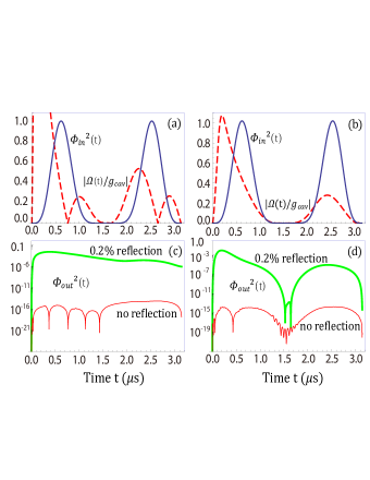
Figure 2: (Color online) Input single photon packet (blue line), the driving pulse (red-dashed line) and ${\left|{{\Phi_{out}}}\right|^{2}}$ as a function of time. The parameters chosen are ${g_{cav}}=30\pi MHz,{\gamma_{L}}=6\pi MHz$. In the numerical simulations here and hereafter, the coupling strength $\Gamma$ is given by Eq. (41). Initially, the system is prepared almost in $\left|{g,0,0}\right\rangle$ with a small probability ${\rho_{offset}}=0.002$ in $\left|{e,0,0}\right\rangle$, which is plotted in (c) and (d)(thin-red lines). For comparison, we plot ${\left|{{\Phi_{out}}}\right|^{2}}$ in (c) and (d)(bold-green lines) for the case in which the system is prepared with probability 1 in $\left|{g,0,0}\right\rangle$. Note that in this case, we still use the driving pulse calculated with ${\rho_{offset}}=0.002$, so the reflection is higher. The other parameters chosen are ${\Delta_{1}}{\rm{=}}{\Delta_{2}}{\rm{=}}0$, $W=1.6716MHz$ for (a) and (c), $W=17.238MHz$ for (b) and (d).

Fig. 2 (a) and (b) show that in order to store the input photon completely, we have to change the driving pulse according to the cavity-input field couplings. From Fig. 2 (c), we can learn that when the initial state of atom matches the conditions used to calculate $\Omega(t)$, i.e., with ${\rho_{offset}}=0.002$, no photon is reflected out (it is below ${10^{-16}}$, almost zero). However, if the initial state deviates from the state used to calculate the driving pulse, say the initial state is $\left|{g,0,0}\right\rangle$, the photon would be reflected off the cavity with an probability of $0.2\%$, which is much larger than ${10^{-16}}$ and can be explained as a mismatch between the initial state used to calculate the driving pulse and the realistic initial state.

In order to compare the results of non-Markovian process with that of Markovian one, we plot the time evolution of the atomic population in the excited state $\left|e\right\rangle$ and the real driving pulse (corresponding to zero detunings) $\Omega(t)$ (42) in Fig. 3. We find that when the coupling $W$ is small (see Fig. 3 (a) and (c)), the so-called back-flowing phenomenon occurs for the population ${\rho_{ee}}$. As $W$ increases, the results given by the non-Markovian Eq. (28) are in good agreement with those given in the Markovian limit (see Fig. 3 (b) and (d)). Besides, from Fig. 4 (a) and (b), we can see that the excited state population ${\rho_{ee}}(t)$ obtained in the non-Markovian case Eq. (28) is different from that ${\rho_{fee}}(t)$ in the Markovian case Eq. (35) when the parameter $W$ runs from $0.5$ to $2$, but the difference is not clear for $W>2$, see Fig. 4 (c) and (d).

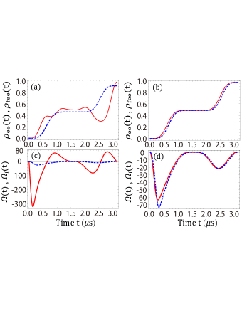
Figure 3: (Color online) The populations of the atom on the excited state ${\rho_{ee}}(t)$ (non-Markovian case) and ${\rho_{fee}}(t)$ (Markovian case), the driving pulse $\Omega(t)$ (non-Markovian case) and ${\Omega_{f}}(t)$ (Markovian case) versus time $t$. The red line denotes the non-Markovian case and the blue-dashed line denotes the Markovian case. Parameters chosen are ${\Delta_{1}}{\rm{=}}{\Delta_{2}}{\rm{=}}0$, ${\rho_{offset}}=0.0075$, ${g_{cav}}=30\pi MHz,{\gamma_{L}}=6\pi MHz.W=0.5MHz,$ for (a) and (c). $W=25MHz$ for (b) and (d).

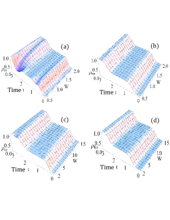
Figure 4: (Color online) The time evolution of the excited state population in non-Markovian limit ${\rho_{ee}}(t)$ and in the Markovian limit ${\rho_{fee}}(t)$ as a function of time $t$ and the coupling strength $W$. Parameters chosen are ${{g_{cav}}=30}\pi MHz,$ ${\gamma_{L}}=6\pi MHz.$

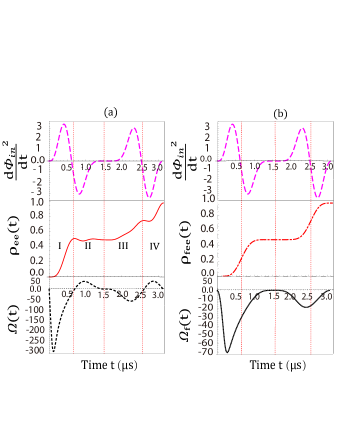
Figure 5: (Color online) Comparison of non-Markovian case to Markovian case in terms of ${\rho}(t)$ and $\Omega(t)$. Parameters chosen are ${\Delta_{1}}{\rm{=}}{\Delta_{2}}{\rm{=}}0$, ${\rm{{g_{cav}}=30}}\pi MHz,{\gamma_{L}}=6\pi MHz,W=1MHz,$ ${\rho_{offset}}=0.004$.

To shed more light on the photon storing in the non-Markovian limit, we compare the non-Markovian results with that in the Markovian case, see Fig. 5 (a). By the input signal ${\left|{{\Phi_{in}}}\right|^{2}}$, we divide the dynamics and the time-dependence of the driving pulse into 4 regimes, labeled by ${\rm I}$, ${\rm II}$, ${\rm III}$ and ${\rm IV}$. In regime ${\rm I}$ and ${\rm III}$, the driving pulse $\Omega(t)$ is negative in both non-Markovian and Markovian cases, while the populations of the atom in the excited state $|e\rangle$ increase continuously in these regimes, i.e., no population backflowing in the dynamics. In contrary, the driving pulse in regime ${\rm II}$ and ${\rm IV}$ are positive, and there are population backflowing in these regimes.

Now we study the effect of detunings ${\Delta_{1}}$ and ${\Delta_{2}}$ on the driving pulse $\Omega(t)$. Examining Eq. (30), we find that $A(t)={\Delta_{1}}t$ and $\Omega(t)={e^{-i{\Delta_{1}}t}}({\partial_{t}}\tilde{X}(t)-{g_{cav}}G(t)+{\gamma_{L}}\tilde{X}(t))$ when the detuning ${\Delta_{2}}=0$. When ${\Delta_{2}}\neq 0$, the modulus $\left|{\Omega(t)}\right|$ of the driving pulse $\Omega(t)$ does not depend on the detuning ${\Delta_{1}}$, while it depends on the absolute value of ${\Delta_{2}}$ only (see Fig. 6). Meanwhile the argument $\theta(t)$ of the $\Omega(t)$ depends on both detunings ${\Delta_{1}}$ and ${\Delta_{2}}$. The argument $\theta(t)$ of the driving pulse ${\Omega(t)}$ is an odd function of ${\Delta_{2}}$ (see Fig. 7 (a) and (b)) when ${\Delta_{1}}=0$ or ${\Delta_{1}}={\Delta_{2}}$.

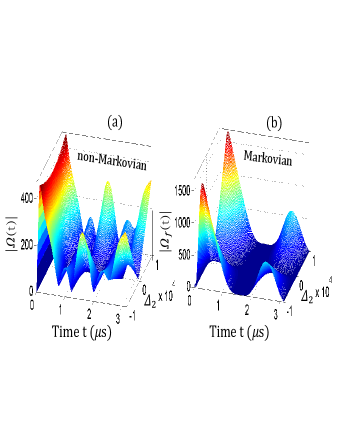
Figure 6: (Color online) The modulus $\left|{\Omega(t)}\right|$ (non-Markovian case, see Eq. (33)) and $\left|{{\Omega_{f}}(t)}\right|$ (Markovian case) of the driving pulse $\Omega(t)$ vary with the detuning ${\Delta_{2}}$ and time $t$. Parameters chosen are ${\rm{{g_{cav}}=30}}\pi MHz,{\gamma_{L}}=6\pi MHz,W=0.5MHz,{\rho_{offset}}=0.003$.

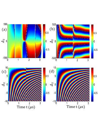
Figure 7: (Color online) The argument $\sin\theta(t)$ ((a) and (c), see Eq. (34)) in the non-Markovian case and $\sin{\theta_{f}}(t)$ ((b) and (d)) in the Markovian case vary with the detuning ${\Delta_{2}}$ and time $t$. Parameters chosen are ${\Delta_{1}}={\Delta_{2}},{\rm{{g_{cav}}=30}}\pi MHz,{\gamma_{L}}=6\pi MHz,W=0.5MHz,{\rho_{offset}}=0.003$, for (a) and (b), and ${\Delta_{1}}=20$, for (c) and (d).

V Photon storing in dark states

We now discuss the problem of transferring a single-photon state of the input field to an atom-cavity dark state, taking the non-Markovian effect into account. We show that these processes can be achieved by adiabatically rotating the cavity dark state in a special way. Before proceeding, we introduce a dark $\left|D(t)\right\rangle$ and its orthogonal bright states $\left|B(t)\right\rangle$Cohen-Tannoudji197710 ; Fleischhauer2000179 ,

$$\left|{D(t)}\right\rangle= -\cos\varphi(t)\left|{g,1,0}\right\rangle+\sin\varphi(t)\left|{e,0,0}\right\rangle,$$ (43)

$$\left|{B(t)}\right\rangle= \sin\varphi(t)\left|{g,1,0}\right\rangle+\cos\varphi(t)\left|{e,0,0}\right\rangle,$$

where $\tan\varphi(t)={g_{cav}}/\Omega(t)$.

Taking the dark and bright states instead of $\left|{g,1,0}\right\rangle$ and $\left|{e,0,0}\right\rangle$ as the basis, we re-expand Eq. (44) as,

$$\left|{\psi(t)}\right\rangle= D(t)\left|D(t)\right\rangle+B(t)\left|B(t)\right\rangle+X(t)\left|{x,0,0}\right\rangle$$ (44)

$$+\int_{-\infty}^{\infty}{d\omega{C_{\omega}}(t){{\hat{b}}^{\dagger}}(\omega)\left|{g,0,0}\right\rangle},$$

The relations between the amplitudes $D(t)$, $B(t)$, $G(t)$ and $E(t)$ can be written as

$$D(t)= -\cos\varphi(t)G(t)+\sin\varphi(t)E(t),$$ (45)

$$B(t)= \sin\varphi(t)G(t)+\cos\varphi(t)E(t).$$

The evolution equations (7) in terms of Eq. (45) then takes (we here consider only the ${\Delta_{1}}={\Delta_{2}}=0$)

$$\dot{X}= -i{\Omega_{1}}(t)B(t)-{\gamma_{L}}X,$$ (46)

$$\dot{D}= \dot{\varphi}B(t)+\cos\varphi\int{d\omega{\kappa^{*}}(\omega){C_{\omega}}},$$

$$\dot{B}= -\dot{\varphi}D(t)-i{\Omega_{1}}(t)X-\sin\varphi\int{d\omega{\kappa^{*}}(\omega){C_{\omega}}},$$

$${{\dot{C}}_{\omega}}= -i{\Omega_{\omega}}{C_{\omega}}+\kappa(\omega)\sin\varphi B(t)-\cos\varphi\kappa(\omega)D(t),$$

where ${\Omega_{1}}(t)=\sqrt{g_{cav}^{2}+{\Omega^{2}}(t)}$, and the terms proportional to $\dot{\varphi}$ describe the coupling between the bright and dark state induced by non-adiabatic evolutions. We now adiabatically eliminate the excited state, this is possible if the characteristic time ${t_{1}}$ of the system is sufficiently longer than the decay time of the excited state (${\gamma_{L}}{t_{1}}\gg 1$). After elimination of the excited state, we adiabatically eliminate the bright-state and neglect terms with $\dot{\varphi}$. The conditions which validate such an elimination will be given later. Defining $D(t)=-{d_{1}}$, we finally arrive atLukin200084 ; Fleischhauer2000179

$$\mathop{{d_{1}}}\limits^{.}= -\cos\varphi(t)\int{d\omega{\kappa^{*}}(\omega){C_{\omega}}(t)},$$ (47)

$${{\dot{C}}_{\omega}}= -i{\Omega_{\omega}}{C_{\omega}}(t)+\cos\varphi(t)\kappa(\omega){d_{1}}(t).$$

One immediately recognizes from these equations that the total probability of finding the system in single photon states of the input field and in the cavity-dark state is conserved

$$\frac{d}{{dt}}\left[{{{\left|{{d_{1}}(t)}\right|}^{2}}+\int{d\omega{{\left|{{C_{\omega}}(t)}\right|}^{2}}}}\right]=0.$$ (48)

Thus with adiabatic evolution, the system can occupy only two states, namely, the input field state and the cavity dark state.

Formally integrating the second equation of Eq. (47) and substituting it into the first (these steps are similar to Eq. (7)-Eq. (13)), we get

$$\mathop{{d_{1}}}\limits^{.}(t)= \cos\varphi(t)N(t)$$ (49)

$$-\cos\varphi(t)\int_{0}^{t}{d\tau\cos\varphi(\tau){d_{1}}(\tau)f(t-\tau)},$$

$${\Phi_{in}}(t)+ {\Phi_{out}}(t)=\int_{0}^{t}{d\tau h(t-\tau)\cos\varphi(\tau){d_{1}}(\tau)}.$$

We note the adiabatic evolution happens whenLukin200084 ; Duan200367 ; Fleischhauer2000179

$$g_{cav}^{2}\gg{\gamma_{L}}\Gamma.$$ (50)

This condition is the same as that for adiabatic storing in the Markovian limit, in other words, the non-Markovian and Markovian systems share the same condition to store a photon adiabatically. Take use of the completely impedance matching condition Eq. (16), we obtain

$$\cos\varphi(t){d_{1}}(t)=G(t).$$ (51)

Substituting Eq. (51) into the first equation of Eq. (49), we get

$${d_{1}}(t)= \sqrt{2\int_{0}^{t}{M(\tau)d\tau}},$$ (52)

$$\Omega(t)= \frac{{{g_{cav}}}}{{\tan\varphi(t)}},$$

where $M(t)=G(t){\rm{N}}(t)-G(t)\int_{0}^{t}G(\tau)f(t-\tau)d\tau,$ $\cos\varphi(t)=\frac{{G(t)}}{{{d_{1}}(t)}}$. In order to compare the analytical results under the adiabatic evolution Eq. (52) with the exact analytical results in Eq. (42) given by

$${D_{dark}}(t)=G(t)\cos{\varphi_{1}}(t)-E(t)\sin{\varphi_{1}}(t),$$ (53)

we plot the time evolution of the population of the dark state and the driving pulse in Fig. 8. Here $G(t)$ and $E(t)=\sqrt{{\rho_{ee}}(t)}$ are the exact analytical expressions in Eq. (54) and Eq. (28), respectively, and ${\varphi_{1}}=arc\tan[{g_{cav}}/\Omega(t)]$ is determined by Eq. (42).

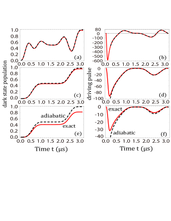
Figure 8: (Color online) This plot shows the comparison of the adiabatic elimination approximation and the exact expression. The red line and black-dashed line denote the exact solution (see Eq. (53) and Eq. (42)) and the solution of adiabatic elimination approximation (see Eq. (52)). Parameters chosen are ${\Delta_{1}}{\rm{=}}{\Delta_{2}}{\rm{=}}0$, ${\rho_{offset}}=0.00075,{\rm{{g_{cav}}=30}}\pi MHz,{\gamma_{L}}=6\pi MHz,W=0.5MHz$ for (a) and (b), ${\rm{{g_{cav}}=30}}\pi MHz,{\gamma_{L}}=6\pi MHz,W=25MHz$ for (c) and (d) and ${{\rm{g}}_{{\rm{cav}}}}{\rm{=14}}\pi{\rm{MHz}},{\gamma_{L}}=6\pi MHz,W=25MHz$ for (e) and (f).

We find from the figure that the results given by the adiabatic elimination Eq. (52) are in good agreement with those obtained by the exact analytical expression Eq. (42) and Eq. (53) when the strong coupling conditions (50) are satisfied (see Fig. 8 (a), (c) and (b), (d)). When the coupling is weak (50) (see Fig. 8 (e) and (f)), the curve obtained by the adiabatic elimination approximation Eq. (52) has serious deviations from those obtained by the exact analytical expression Eq. (42) and Eq. (53). In addition, from Fig. 8 (b), (d), and (f), we can see that the driving pulse $\Omega(t)$ obtained by the adiabatic elimination Eq. (52) shows serious deviations from those obtained by the exact analytical expression Eq. (42) when the time is short (approximately $t=0.2\mu s$), this can be explained as an effect of the imperfect impedance matching, in other words, with ${\rho_{offset}}=0$ the perfect impedance matching can take place only with $\Omega(t)\rightarrow\infty$.

From Fig. 8 (a) and (b), we can learn that the non-Markovianity caused backflowing to the dark state occurs when the parameter $W$ is small. The non-Markovian regime transits to the Markovian regime when the parameter $W$ is large. Therefore by manipulating $W$ we can control the crossover from a non-Markovian process to a Markovian process and verse visa, this provides us with photon storing in the atom-cavity system in both non-Markovian and Markovian limits.

VI Conclusion

The storing of a single photon of arbitrary temporal shape in a single three-level atom coupled to an optical cavity in non-Markovian dynamics has been explored. To calculate the driving pulse, we first extend the input-output relation from Markovian to non-Markovian process, taking the off-resonant couplings between the atom and fields into account. With the extended input-output relation, we have presented a very simple recipe for calculating the driving pulse with non-zero detunings ${\Delta_{1}}$ and ${\Delta_{2}}$, and discuss the features caused by the non-Markovian effect. We also present a proposal to store the single photon in a dark state of the cavity-atom system by adiabatically steering the dark state. In addition, due to the constraint relationship on the strength $\Gamma$ of the coupling and the bandwidth $W$ decided by Eq. (41) , we only discuss the dependence of the non-Markovian effects of the dynamics on the value of the parameter W and find that the jumping continuously from the non-Markovian regime to Markovian regime is got through manipulating width W of the band of the effective spectral density.

VII acknowledgments

This work is supported by the NSF of China under Grants Nos 61078011, 10935010 and 11175032.

Appendix A Calculational details of the population of the atom in the excited state and the complex driving pulse with the detunings

A.1 The population of the atom in the excited state

Substituting Eq. (21) and Eq. (16) into the first and fourth equation of Eq. (13), we obtain

$$G(t)=\frac{{{{\dot{\Phi}}_{in}}(t)+W{\Phi_{in}}(t)}}{{W\sqrt{\Gamma}}},$$ (54)

and

$$\tilde{X}(t)=[-\dot{G}(t)+N(t)-\int_{0}^{t}{d\tau f(t-\tau)G(\tau)}]/{g_{cav}},$$ (55)

here, $\tilde{X}(t)=i{e^{-i{\Delta_{2}}t}}X(t)$. We note that the envelope ${\Phi_{in}}(t)$ of the input is a real function of time, so both $G(t)$ and ${\tilde{X}}$ are real. Defining $E(t)={e^{-i{\Delta_{1}}t+i{\Delta_{2}}t}}\tilde{E}(t)$, we have from Eq. (7)

$$\Omega(t)\tilde{E}(t)={\partial_{t}}\tilde{X}(t)+i{\Delta_{2}}\tilde{X}(t)-{g_{cav}}G(t)+{\gamma_{L}}\tilde{X}(t),$$ (56)

and

$${\Omega^{*}}(t)\tilde{X}(t)=-i\Delta\tilde{E}(t)-{\partial_{t}}\tilde{E}(t),$$ (57)

where $\Delta={\Delta_{2}}-{\Delta_{1}}$. It is easy to find that ${\tilde{E}(t)}$ and $\Omega(t)$ are complex due to nonzero detunings ${\Delta_{1}}$ and ${\Delta_{2}}$, this is one of the differences between our work and the earlier oneDilley201285 . Taking a complex conjugation of both sides of Eq. (56) yields,

$$\Omega{{(t)}^{*}}{{\tilde{E}}^{*}}(t)= {\partial_{t}}\tilde{X}(t)-i{\Delta_{2}}\tilde{X}(t)$$ (58)

$$-{g_{cav}}G(t)+{\gamma_{L}}\tilde{X}(t).$$

Dividing Eq. (57) by Eq. (58), we have

$$-i\Delta{\left|{E(t)}\right|^{2}}-{{\tilde{E}}^{*}}(t){\partial_{t}}\tilde{E}(t)=\tilde{X}(t){\partial_{t}}\tilde{X}(t)$$ (59)

$$-i{\Delta_{2}}{{\tilde{X}}^{2}}(t)-{g_{cav}}\tilde{X}(t)G(t)+{\gamma_{L}}{{\tilde{X}}^{2}}(t).$$

Taking the complex conjugation of both sides of Eq. (57), we have

$${\Omega(t)\tilde{X}(t)=i\Delta{{\tilde{E}}^{*}}(t)-{\partial_{t}}{{\tilde{E}}^{*}}(t).}$$ (60)

Dividing Eq. (56) by Eq. (60), we have

$$-i\Delta{{\left|{E(t)}\right|}^{2}}+\tilde{E}(t){\partial_{t}}{{\tilde{E}}^{*}}(t)=-\tilde{X}(t){\partial_{t}}\tilde{X}(t)$$ (61)

$$-i{\Delta_{2}}{{\tilde{X}}^{2}}(t)+{g_{cav}}\tilde{X}(t)G(t)-{\gamma_{L}}{{\tilde{X}}^{2}}(t).$$

Using Eq. (61), Eq. (59) and ${\partial_{t}}{\rho_{ee}}(t)=\tilde{E}(t){\partial_{t}}{\tilde{E}^{*}}(t)+{\tilde{E}^{*}}(t){\partial_{t}}\tilde{E}(t)$, we get a differential equation of ${\rho_{ee}}(t)$

$${{\dot{\rho}}_{ee}}(t)= -2\tilde{X}(t){\partial_{t}}\tilde{X}(t)+2{g_{cav}}\tilde{X}(t)G(t)$$ (62)

$$-2{\gamma_{L}}{{\tilde{X}}^{2}}(t).$$

Therefore, Eq. (28) is obtained by formally integrating Eq. (62).

A.2 The complex driving pulse with the detunings

Multiplying both sides of Eq. (61) by $-i$ and taking the complex conjugation of the result, we obtain

$$-\Delta{{\left|{\tilde{E}(t)}\right|}^{2}}+i{{\tilde{E}}^{*}}(t){\partial_{t}}\tilde{E}(t)=-i\tilde{X}(t){\partial_{t}}\tilde{X}(t)$$ (63)

$$-{\Delta_{2}}{{\tilde{X}}^{2}}(t)+i{g_{cav}}\tilde{X}(t)G(t)-i{\gamma_{L}}{{\tilde{X}}^{2}}(t).$$

Considering

$${{\tilde{E}}^{*}}(t)= \frac{{{\rho_{ee}}(t)}}{{\tilde{E}(t)}},$$ (64)

$${\rho_{ee}}(t)= {\left|{\tilde{E}(t)}\right|^{2}},$$

substituting Eq. (64) into Eq. (63) and formally integrating the obtained result from $0$ to $t$, we arrive at

$$\tilde{E}(t)=\tilde{E}(0)\exp\int_{0}^{t}{dt^{\prime}\{[\Delta{\rho_{ee}}(t^{\prime})-i\tilde{X}(t^{\prime}){\partial_{t^{\prime}}}\tilde{X}(t^{\prime})-}$$ (65)

$${\Delta_{2}}{{\tilde{X}}^{2}}(t^{\prime})+i{g_{cav}}\tilde{X}(t^{\prime})G(t^{\prime})-i{\gamma_{L}}{{\tilde{X}}^{2}}(t^{\prime})]/(i{\rho_{ee}}(t^{\prime})\},$$

where $\tilde{E}(0)=\sqrt{{\rho_{offset}}}$ representing the initial offset, i.e., the probability amplitude of finding the system in the excited state. Finally, we can obtain Eq. (29) by substituting Eq. (65) into Eq. (56) and separating the real and imaginary part of the complex driving pulse ${\Omega(t)}$.

References

- (1) D. P. DiVincenzo, Nature 393, 113 (1998).
- (2) E. Knill, R. Laflamme, and G. J. Milburn, Nature 409, 46 (2001).
- (3) J. I. Cirac, A. K. Ekert, S. F. Huelga, and C. Macchiavello, Phys. Rev. A 59, 4249 (1999).
- (4) D. P. DiVincenzo, Fortschr. Phys. 48, 771 (2000).
- (5) J. I. Cirac, P. Zoller, H. J. Kimble, and H. Mabuchi, Phys. Rev. Lett. 78, 3221 (1997).
- (6) L.-M. Duan, A. Kuzmich, and H. J. Kimble, Phys, Rev, A 67, 032305 (2003).
- (7) R.-B. Liu, W. Yao, and L. J. Sham, Adv. Phys. 59, 703 (2010).
- (8) M. Oxborrow and A. G. Sinclair, Contemp. Phys. 46, 173 (2005).
- (9) C. K. Law and H. J. Kimble, J. Mod. Opt. 44, 2067 (1997).
- (10) A. Kuhn, M. Hennrich, T. Bondo, and G. Rempe, Appl. Phys. B 69, 373 (1999).
- (11) A. Kuhn , M. Hennrich, and G. Rempe, Phys. Rev. Lett. 89, 067901 (2002).
- (12) B. Sun, M. S. Chapman, and L. You, Phys. Rev. A 69, 042316 (2004).
- (13) J. McKeever, A. Boca, A. D. Boozer, R. Miller, J. R. Buck, A. Kuzmich, and H. J. Kimble, Science 303, 1992 (2004).
- (14) M. Keller, B. Lange, K. Hayasaka, W. Lange, and H. Walther, Nature 431, 1075 (2004).
- (15) T. Legero, T. Wilk, M. Hennrich, G. Rempe, and A. Kuhn, Phys. Rev. Lett. 93, 070503 (2004).
- (16) H. J. Carmichael, An Open Systems Approach to Quantum Optics, Lecture Notes in Physics, Vol. m18 (Springer-Verlag, Berlin, 1993).
- (17) M. J. Hartmann, F. G. S. L. Brandao, and M. B. Plenio, Nature Phys. 2, 849 (2006).
- (18) T. Pellizzari, Phys. Rev. Lett. 79, 5242 (1997).
- (19) A. Biswas and D. A. Lidar, Phys. Rev. A 74, 062303 (2006).
- (20) Q. A. Turchette, C. J. Myatt, B. E. King, C. A. Sackett, D. Kielpinski, W. M. Itano, C. Monroe, and D. J. Wineland, Phys. Rev. A 62, 053807 (2000).
- (21) C. J. Myatt, B. E. King, Q. A. Turchette, C. A. Sackett, D. Kielpinski, W. M. Itano, C. Monroe, and D. J. Wineland, Nature (London) 403, 269 (2000).
- (22) S. Maniscalco, J. Piilo, F. Intravaia, F. Petruccione, and A. Messina, Phys. Rev. A 69, 052101 (2004).
- (23) N. Stefanou and A. Modinos, Phys. Rev. B 57, 12127 (1998).
- (24) M. Bayindir, B. Temelkuran, and E. Ozbay, Phys. Rev. Lett. 84, 2140 (2000).
- (25) Y. Xu, Y. Li, R. K. Lee, and A. Yariv, Phys. Rev. E 62, 7389 (2000).
- (26) L.-L. Lin, Z.-Y. Li, and B. lin, Phys. Rev. B 72, 165330 (2005).
- (27) S. Longhi, Phys. Rev. A 74, 063826 (2006).
- (28) W. Yao, R.-B Liu, and L. J. Sham, Phys. Rev. Lett. 95, 030504 (2005).
- (29) M. D. Lukin, S. F. Yelin, and M. Fleischhauer, Phys. Rev. Lett. 84, 4232 (2000).
- (30) M. Fleischhauer, S. F. Yelin, and M. D. Lukin, Opt. Commun. 179, 395 (2000).
- (31) J. Dilley, P. Nisbet-Jones, B. W. Shore, and A. Kuhn, Phys. Rev. A 85, 023834 (2012).
- (32) F.-Y. Hong and S.-J. Xiong, Phys. Rev. A 76, 052302 (2007).
- (33) J. Piilo, S. Maniscalco, K. Härkönen, and K.-A. Suominen, Phys. Rev. Lett. 100, 180402 (2008).
- (34) J. Piilo, K. Härkönen, S. Maniscalco, and K.-A. Suominen, Phys. Rev. A 79, 062112 (2009).
- (35) S. Maniscalco and F. Petruccione, Phys. Rev. A 73, 012111 (2006).
- (36) B. Bellomo, R. L. Franco, and G. Compagno, Phys. Rev. Lett. 99, 160502 (2007).
- (37) C. W. Gardiner and P. Zoller, Quantum Noise (Springer-Verlag, Berlin, Germany, 2000).
- (38) M. O. Scully and M. S. Zubairy, Quantum Optics (Cambridge University Press, Cambridge, UK, 1997).
- (39) D. F. Walls and G. J. Milburn, Quantum Optics (Springer-Verlag, Berlin, 1994).
- (40) M. A. Nielsen and I. L. Chuang, Quantum Computation and Quantum information (Cambridge University Press, Cambridge, UK, 2000).
- (41) C. H. Bennett and D. P. DiVincenzo, Nature (London) 404, 247 (2000).
- (42) J. Zhang, Y.-X. Liu, R.-B. Wu, K. Jacobs, and F. Nori, Phys. Rev. A 87, 032117 (2013).
- (43) C. W. Gardiner and M. J. Collett, Phys. Rev. A 31, 3761 (1985).
- (44) G. S. Vasilev, D. Ljunggren, and A. Kuhn, New J. Phys. 12, 063024 (2010).
- (45) P. Haikka and S. Maniscalco, Phys. Rev. A 81, 052103 (2010).
- (46) H.-P. Breuer and F. Petruccione, The Theory of Open Quantum Systems (Oxford University Press, Oxford, UK, 2002)
- (47) H.-N. Xiong, W.-M. Zhang, M. W. Y. Tu, and D. Braun, Phys. Rev. A 86, 032107 (2012).
- (48) M. W. Jack, M. J. Collett, and D. F. Walls, Phys. Rev. A 59, 2306 (1999).
- (49) T. Yu, L. Diósi, N. Gisin, and W. T. Strunz, Phys. Rev. A 60, 91 (1999).
- (50) C. Cohen-Tannoudji, and S. Reynaud, J. Phys. B 10, 2311 (1977).