GPU acceleration of Newton’s method
for large systems of polynomial equations
in double double and quad double arithmetic

Abstract

In order to compensate for the higher cost of double double and quad double arithmetic when solving large polynomial systems, we investigate the application of NVIDIA Tesla K20C general purpose graphics processing unit. The focus on this paper is on Newton’s method, which requires the evaluation of the polynomials, their derivatives, and the solution of a linear system to compute the update to the current approximation for the solution. The reverse mode of algorithmic differentiation for a product of variables is rewritten in a binary tree fashion so all threads in a block can collaborate in the computation. For double arithmetic, the evaluation and differentiation problem is memory bound, whereas for complex quad double arithmetic the problem is compute bound. With acceleration we can double the dimension and get results that are twice as accurate in about the same time.

Key words and phrases. compute unified device architecture (CUDA), double double arithmetic, differentiation and evaluation, general purpose graphics processing unit (GPU), Newton’s method, least squares, massively parallel algorithm, modified Gram-Schmidt method, polynomial evaluation, polynomial differentiation, polynomial system, QR decomposition, quad double arithmetic, quality up.

1 Introduction

We investigate the application of general purpose graphics processing units (GPUs) to solving large systems of polynomial equations with numerical methods. Large systems not only lead to an increased number of operations, but also to more accumulation of numerical roundoff errors and therefore to the need to calculate in a precision that is higher than the common double precision. Motivated by the need of higher numerical precision, we can formulate our goal more precisely. With massively parallel algorithms we aim to offset the extra cost of double double and quad double arithmetic [20, 27] and achieve quality up [3], a project we started in [36].

Problem Statement. Our problem is to accelerate Newton’s method for large polynomial systems, aiming to offset the overhead cost of double double and quad double complex arithmetic. We assume the input polynomials are given in their sparse distributed form: all polynomials are fully expanded and only those monomials that have a nonzero coefficient are stored. For accuracy and application to overdetermined systems, we solve linear systems in the least squares sense and implement the method of Gauss-Newton.

Our original massively parallel algorithms for evaluation and differentiation of polynomials [37] and for the modified Gram-Schmidt method [38] were written with a fine granularity, making intensive use of the shared memory. The limitations on the capacity of the shared memory led to restrictions on the dimensions on the problems we could solve. These problems worsened for higher levels of precision, in contrast to the rising need for more precision in higher dimensions.

Related Work. As the QR decomposition is of fundamental importance in applied linear algebra many parallel implementations have been investigated by many authors, see e.g. [2], [4]. A high performance implementation of the QR algorithm on GPUs is described in [23]. In [8], the performance of CPU and GPU implementations of the Gram-Schmidt were compared. A multicore QR factorization is compared to a GPU implementation in [28]. GPU algorithms for approaches related to QR and Gram-Schmidt are for lattice basis reduction [5] and singular value decomposition [13]. In [39], the left-looking scheme is dismissed because of its limited inherent parallelism and as in [39] we also prefer the right-looking algorithm for more thread-level parallelism.

The application of extended precision to BLAS is described in [26], see [11] for least squares solutions. The implementation of BLAS routines on GPUs in triple precision (double + single float) is discussed in [31]. In [32], double double arithmetic is described under the section of error-free transformations. An implementation of interval arithmetic on CUDA GPUs is presented in [9].

The other computationally intensive stage in the application of Newton’s method is the evaluation and differentiation of the system. Parallel automatic differentiation techniques are described in [6], [16], and [34].

Concerning the GPU acceleration of polynomial systems solving, we mention two recent works. A subresultant method with a CUDA implementation of the FFT to solve systems of two variables is presented in [29]. In [25], a CUDA implementation for an NVIDIA GPU of a multidimensional bisection algorithm is discussed.

Our contributions. For the polynomial evaluation and differentiation we reformulate algorithms of algorithmic differentiation [17] applying optimized parallel reduction [18] to the products that appear in the reverse mode of differentiation. Because our computations are geared towards extended precision arithmetic which carry a higher cost per operation, we can afford a fine granularity in our parallel algorithms. Compared to our previous GPU implementations in [37, 38], we have removed the restrictions on the dimensions and are now able to solve problems involving several thousands of variables. The performance investigation involves mixing the memory-bound polynomial evaluation and differentiation with the compute-bound linear system solving.

2 Polynomial Evaluation and Differentiation

We distinguish three tasks in the evaluation and differentiation of polynomials in several variables given in their sparse distributed form. First, we separate the high degree parts into common factors and then apply algorithmic differentiation to products of variables. In the third stage, monomials are multiplied with coefficients and the terms are added up.

2.1 common factors and tables of power products

A monomial in $n$ variables is defined by a sequence of natural numbers $d_{i}\geq 0$, for $i=1,2,\ldots,n$. We decompose a monomial as follows:

$$x_{1}^{d_{1}}x_{2}^{d_{2}}\cdots x_{n}^{d_{n}}=x_{i_{1}}x_{i_{2}}\cdots x_{i_{k}}\times x_{j_{1}}^{e_{j_{1}}}x_{j_{2}}^{e_{j_{2}}}\cdots x_{j_{\ell}}^{e_{j_{\ell}}}$$ (1)

where $x_{i_{1}}x_{i_{2}}\cdots x_{i_{k}}$ is the product of all $k$ variables that have a nonzero exponent. The $\ell$ variables that appear with a positive exponent occur in $x_{j_{1}}^{e_{j_{1}}}x_{j_{2}}^{e_{j_{2}}}\cdots x_{j_{\ell}}^{e_{j_{\ell}}}$ with exponent $e_{j_{i}}=d_{j_{i}}-1$, for $i=1,2,\ldots,\ell$.

We call the monomial $x_{j_{1}}^{e_{j_{1}}}x_{j_{2}}^{e_{j_{2}}}\cdots x_{j_{\ell}}^{e_{j_{\ell}}}$ a common factor, as this factor is a factor in all partial derivatives of the monomial. Using tables of pure powers of the variables, the values of the common factors are products of the proper entries in those tables. The cost of evaluating monomials of high degrees is thus deferred to computing powers of the variables. The table of pure powers is computed in shared memory by each block of threads.

2.2 evaluation and differentiation of a product of variables

Consider a product of variables: $x_{1}\star x_{2}\star\cdots\star x_{n}$. The straightforward evaluation and the computation of the gradient takes $n-1+n\times(n-2)=n^{2}-n-1$ multiplications. Recognizing the product as the example of Speelpenning in algorithmic differentiation [17], the number of multiplications to evaluate the product and compute all its derivatives drops to $3n-5$.

The computation of the gradient requires in total $n-1$ extra memory locations. We need $n-2$ locations for the intermediate forward products $x_{1}\star x_{2}\star\cdots\star x_{k}$, $k=2,3,\ldots,n-1$. For the backward products $x_{n}\star x_{n-1}\star\cdots\star x_{k}$, $k=n-1,n-2,\ldots,3$ only one extra temporary memory location is needed, as this location can be reused each time for the next backward product, if the computation of the backward products is interlaced with the multiplication of the forward with the corresponding backward product.

For $n=4$, Figure 1 displays two arithmetic circuits, one to evaluate a product of variables and another to compute its gradient. The second circuit is executed after the first one, using the same tree structure that holds intermediate products. At a node in a circuit, we write $x_{1}\star x_{2}$ if the multiplication $\star$ happens at the node and we write $x_{1}x_{2}$ if we use the value of the product. At most one multiplication is performed at each node of the circuit.

Figure 1: The left picture shows the evaluation of a product of variables organized in a binary tree, starting at the leaves and placing the result at the root of the tree. The picture at the right shows the computation of all derivatives (the gradient), with inputs taken from different levels in the tree. We count 3 $\star$ to evaluate and 4 more $\star$ to differentiate.

Denote by $x_{i:j}$ the product $x_{i}\star\cdots\star x_{k}\star\cdots\star x_{j}$, for all natural numbers $k$ between $i$ and $j$. Figure 2 displays the arithmetic circuit to compute all derivatives of a product of 8 variables, after the evaluation of the product in a binary tree.

Figure 2: In the arithmetic circuit to differentiate a product of 8 variables, the inputs are the 8 variables: $x_{1}$, $x_{2}$, $\ldots$, $x_{8}$; the 4 products of 2 consecutive variables: $x_{1:2}$, $x_{3:4}$, $x_{5:6}$, and $x_{7:8}$; and the 2 products of 4 consecutive variables: $x_{1:4}$ and $x_{5:8}$. The nodes $x_{1:4}$ and $x_{5:8}$ have $x_{1:8}$ (omitted because not used) as their common ancestor, which is the root of the tree representation of the differentiation circuit.

To count the number of multiplications to evaluate, we restrict to the case of a complete binary tree, i.e.: $n=2^{k}$ for some $k>0$ and compute the sum $\displaystyle 1+2+4+\cdots+n/2=\sum_{i=0}^{n/2}2^{i}=n-1$. The circuit to compute all derivatives contains a tree of the same size: with $n-1$ nodes, so the number of multiplications equals $n-1$ minus 3 for the nodes closest to the root which require no computations, and plus $n$ for the multiplications at the leaves: $2n-4$ in total. So the total number of multiplications to evaluate a product of $n$ variables and compute its gradient with a binary tree equals $3n-5$.

While keeping the same operational cost of $2n-5$ as the original algorithm, the organization of the multiplication in a binary tree incurs less roundoff. In particular the roundoff error for the evaluated product will be proportional to $\log_{2}(n)$ instead of $n$ of the straightforward multiplication. For a large number of variables, such as $n=1,024$, this reorganization improves the accuracy by two decimal places. The improved accuracy of the evaluated product does not cost more storage as the size of binary tree equals $n-1$.

For the derivatives, the roundoff error is bounded by the number of levels in the arithmetic circuit, which is
$\displaystyle\sum_{k=1}^{\log_{2}(n)}k=\frac{1}{2}(\log_{2}(n))^{2}+\log_{2}(n)$. While this bound is still better than $n-1$, the improved accuracy for the gradient comes at the extra cost of $n-4$ additional memory locations, needed as nodes in the arithmetic circuit for the gradient. In shared memory, the memory locations for the input variables $x_{k}$ are overwritten by the corresponding components of the gradient, e.g.: $x_{1}\star x_{2}\cdots x_{n}$ then occupies the location of $x_{1}$.

In the original formulation of the computation of the example of Speelpenning, only one thread performed all computation for one product and the parallelism consisted in having enough monomials in the system to occupy all threads working separately on different monomials. The reformulation of the evaluation and differentiation with a binary tree allows for several threads to collaborate on the computation of one large product. The reformulation refined the granularity of the parallel algorithm and we applied the techniques suggested in [18].

If $n$ is not a power of 2, then for some positive $k$ and $\ell$, denote $n=2^{k}+\ell<2^{k+1}$. The first $\ell$ threads load two variables and are in charge of the product of those two variables, while other threads load just one variable. The multiplication of values for variables of consecutive index, e.g.: $x_{1}\star x_{2}$ will result in a bank conflict in shared memory as threads require data from an even and odd bank. To avoid bank conflicts, the computations are rearranged, e.g. as $(x_{1}\star x_{3})\star(x_{2}\star x_{4})$, so thread 0 operates on $x_{1},x_{3}$ and thread 1 on $x_{2},x_{4}$.

Table 1 shows the results on the evaluation and differentiation of products of variables in double arithmetic, applying the techniques of [18]. The first GPU algorithm is the reverse mode algorithm that takes $3n-5$ operations executed by one thread per monomial. When all threads in a block collaborate on one monomial in the second GPU algorithm we observe a significant speedup. Speedups and memory bandwidth improve when resolving the bank conflicts in the third improvement. The best results are obtained adding unrolling techniques.

Table 1: Evaluation and differentiation of 65,024 monomials in 1,024 doubles. Times on the K20C obtained with nvprof (the NVIDIA profiler) are in milliseconds (ms). Dividing the number of bytes read and written by the time gives the bandwidth. Times on the CPU are on one 2.6GHz Intel Xeon E5-2670, with code optimized with the -O2 flag.

	method	time	bandwidth	speedup
CPU		330.24ms
GPU	one thread per monomial	86.43ms		3.82
	one block per monomial	15.54ms	79.81GB/s	21.25
	sequential addressing	14.08ms	88.08GB/s	23.45
	unroll last wrap	10.19ms	121.71GB/s	32.40
	complete unroll	9.10ms	136.28GB/s	36.29

In Table 1, one block of threads computes the value and the gradient of one product in 1,024 variables. Instead of one large product, with our code one block can compute many monomials of smaller sizes. In the arithmetic circuits of Figure 1 and 2, instead of going all the way to the root of the tree, the computation stops at some intermediate level. Table 2 present timings for this computation.

Table 2: Evaluation and differentiation of $m$ monomials of different size $n$ by 65,024 blocks with 512 threads per block for 1,024 doubles in shared memory, accelerated by the K20C with timings in milliseconds obtained by the NVIDIA profiler. Times on the CPU are on one 2.6GHz Intel Xeon E5-2670, with code optimized with the -O2 flag.

$n$	$m$	CPU	GPU	speedup
1024	1	330.24ms	9.12ms	36.20
512	2	328.92ms	8.73ms	37.66
256	4	320.78ms	8.84ms	36.29
128	8	309.02ms	8.15ms	37.89
64	16	289.30ms	7.27ms	39.77
32	32	256.07ms	9.51ms	26.94
16	64	230.34ms	8.86ms	25.99
8	128	218.74ms	7.79ms	28.07
4	256	202.20ms	7.05ms	28.69

The evaluation and differentiation of products of variables is memory bound for complex double arithmetic and the techniques illustrated by Table 1 are also relevant for real double double arithmetic. In complex double double and quad double arithmetic, the cost overhead of the arithmetic dominates, the computation becomes compute bound and we use global memory.

2.3 coefficient multiplication and term summation

The third task is to multiply every derivative of the product of variables with the common factor and the proper coefficient, multiplied with the values of the exponents. Then a sum reduction of the evaluated terms gives the values of the polynomials and the Jacobian matrix. The efficient implementation of the scan with CUDA is described in [19].

3 Orthogonalization and Delayed Normalization

Before describing our massively parallel algorithms for the modified Gram-Schmidt method, we formalize the notations. We typically compute with complex numbers and follow notations in [14] for the complex conjugated inner product ${\bf x}^{H}{\bf y}$. Pseudo code of the modified Gram-Schmidt orthogonalization method is listed in Figure 3.

Input: $A\in{\mathbb{C}}^{m\times n}$.
Out	put	:	$Q\in{\mathbb{C}}^{m\times n}$, $R\in{\mathbb{C}}^{n\times n}$: $Q^{H}Q=I$,
			$R$ is upper triangular, and $A=QR$.
let ${{\bf a}}_{k}$ be column $k$ of $A$
for $k$ from 1 to $n$ do
	$r_{k,k}:=\sqrt{{\bf a}_{k}^{H}{\bf a}_{k}}$
	${\bf q}_{k}:={\bf a}_{k}/r_{k,k}$, ${\bf q}_{k}$ is column $k$ of $Q$
	for $j$ from $k+1$ to $n$ do
		$r_{k,j}:={\bf q}_{k}^{H}{\bf a}_{j}$
		${\bf a}_{j}:={\bf a}_{j}-r_{k,j}{\bf q}_{k}$

Figure 3: The modified Gram-Schmidt orthogonalization algorithm.

The modified Gram-Schmidt method computes the the QR decomposition of a matrix $A$, which allows to solve the linear system $A{\bf x}={\bf b}$ in the least squares sense, minimizing $||{\bf b}-A{\bf x}||_{2}^{2}$. In the reduction of $A{\bf x}={\bf b}$ to an upper triangular system $R{\bf x}=Q^{H}{\bf b}$, we do not compute $Q^{H}{\bf b}$ separately. As recommended in [21, §19.3] for numerical stability the modified Gram-Schmidt method is applied to the matrix $A$ augmented with ${\bf b}$:

$$\left[\begin{array}[]{cc}A&{\bf b}\end{array}\right]=\left[\begin{array}[]{cc}Q&{\bf q}_{n+1}\end{array}\right]\left[\begin{array}[]{cc}R&{\bf y}\\ 0&z\end{array}\right].$$ (2)

Because ${\bf q}_{n+1}$ is orthogonal to the column space of $Q$: $||{\bf b}-A{\bf x}||_{2}^{2}=||R{\bf x}-{\bf y}||_{2}^{2}+z^{2}$ and ${\bf y}=Q^{H}{\bf b}$. As a check on the correctness and the accuracy of our computed results, we wrote code to compute $A-QR$. Although computing the entire $A-QR$, the test whether $a_{m,n}-{\bf q}_{n}^{H}{\bf r}_{n}$ is small enough (where ${\bf r}_{n}$ is the last column of $R$) could already indicate whether the working precision was sufficient.

The algorithm in Figure 3 starts with the computation of the complex conjugated inner product ${\bf a}_{k}^{H}{\bf a}_{k}$, followed by the normalization ${\bf q}_{k}:={\bf a}_{k}/r_{k,k}$, where $r_{k,k}:=\sqrt{{\bf a}_{k}^{H}{\bf a}_{k}}$. For the inner product, we load the components of an $m$-dimensional vector into shared memory. Denoting the number of components that fit into the shared memory by $K$ (its capacity), then let $L=\lceil m/K\rceil$ be the number of rounds it takes to compute

$${\bf a}_{k}^{H}{\bf a}_{k}=\sum_{i=0}^{L-1}\sum_{j=0}^{K-1}\overline{a}_{k,iK+j}\star a_{k,iK+j},$$ (3)

where the indexing of the components of a vector starts at zero and $\overline{a}$ denotes the complex conjugate of $a\in{\mathbb{C}}$. The value for $K$ is typically a multiple of the warp size and equals the number of threads in a block. In (3), the index $j$ is the index of the thread in a block, so the inner loop is performed simultaneously in one step by all threads in the block. The outside loop on $i$ is done in a sum reduction and takes $\log_{2}(L)$ steps. The computation of ${\bf a}_{k}^{H}{\bf a}_{k}$ for an $n$-dimensional vector ${\bf a}_{k}$ is reduced to $m$ memory accesses, $L$ steps to make all partial sums $\displaystyle\sum_{j=0}^{K-1}\overline{a}_{k,iK+j}\star a_{k,iK+j}$, and then $\log_{2}(L)$ steps for the outer sum.

When $\star$ is performed in standard precision with hardware arithmetic, then (3) seems to be memory bound, but for the $\star$ in double double and quad double precision, performed by arithmetic encoded in the software, the inner product becomes compute bound as the compute to memory access ratio becomes large enough to offset memory accesses.

For the reduction, we compute the inner product $r_{k,j}:={\bf q}_{k}^{H}{\bf a}_{j}$ of two $m$-vectors:

$$\begin{array}[]{c}{\bf q}_{k}\\ \left[\begin{array}[]{c}q_{k,0}\\ q_{k,1}\\ \vdots\\ q_{k,m-1}\end{array}\right]\end{array}~{}\begin{array}[]{c}{\bf a}_{j}\\ \left[\begin{array}[]{c}a_{j,0}\\ a_{j,1}\\ \vdots\\ a_{j,m-1}\end{array}\right]\end{array}~{}\begin{array}[]{c}{\bf q}_{k}^{H}{\bf a}_{j}\\ \left[\begin{array}[]{c}\bar{q}_{k,0}\star a_{j,0}\\ \bar{q}_{k,1}\star a_{j,1}\\ \vdots\\ \bar{q}_{k,K-1}\star a_{j,m-1}\end{array}\right]\end{array}$$ (4)

As we can keep $K$ components of each vector in shared memory, thread $t$ in a block computes $\bar{q}_{k,t}\star a_{j,t}$. If we may override ${\bf q}_{k}$, then $2m$ shared memory locations suffice, but we still need ${\bf q}_{k}$ for ${\bf a}_{j}:={\bf a}_{j}-r_{k,j}{\bf q}_{k}$. In total we need $3m$ shared memory locations to perform the reductions. Similar to the inner product for the norm of ${\bf a}_{k}$, the computation of ${\bf q}_{k}^{H}{\bf a}_{j}$ is performed in $L$ rounds, where $L=\lceil 3m/K\rceil$, for the capacity $K$ of shared memory.

The calculation of the inner products in $L$ rounds is the first modification to our original massively parallel Gram-Schmidt implementation. The second modification is the delay of the normalization. In the next paragraph we explain the need for this delay.

In the reduction stage, the inner $j$-loop is executed by $n-k$ blocks of threads. Every block of threads performs the normalization of the $k$-th pivot column before proceeding to the reduction. The first block writes the normalized vector into global memory, all other blocks write the reduced vectors into global memory. In the new revised implementation, each vector is processed in several rounds and is read from global memory into shared memory not only at the beginning of the calculations. For large dimensions, not all blocks can be launched simultaneously. It may even be that the block that will reduce the last column is not even scheduled for launching at a time when the first block has finished its writing of the normalized ${\bf a}_{k}$ into global memory.

As some block would load in (partially) normalized vectors in the reduction stage, we propose to delay the normalization to the next iteration of the $k$-loop in the algorithm in Figure 3. At each iteration, the first block writes the norm of the current pivot column to a location in global memory and normalizes the previous pivot column, dividing every component of the previous pivot column by its norm stored in global memory and writes then the normalized previous column into global memory. With delayed normalization, the column ${\bf q}_{k}$ is computed last and is only stored in step $k+1$. At the very end of the algorithm, there is one extra kernel launch for the normalization that leads to ${\bf q}_{n}$.

The application of shared memory to reduce global memory traffic is referred to as tiling [24, pages 108-109]. Our tiles consist of slices of one column as we assign one column to one block. If we want to reduce the number of kernel launches, we could assign multiple (adjacent) columns to one block to make proper tiles as submatrices of the original matrix.

Our implementation of the modified Gram-Schmidt method is a right-looking algorithm, as this gives the most thread-level parallelism, pointed out in [39]. Using a right-looking algorithm, we launch as many blocks as there are columns to update, where each block can work on one column. The cost of memory traffic is mitigated with shared memory and for double double and quad double precision, the cost of the software arithmetic dominates the cost of memory accesses so good speedups are obtained over optimized serial code.

The third modification concerns the back substitution to compute the least squares solution to $Rx=Q^{H}{\bf b}$. Limited by the capacities of shared memory in our previous implementation only one block of threads performed the back substitution. For larger dimensions, denoting $Q^{H}{\bf b}$ by ${\bf y}$, the computation of

$$r_{\ell,\ell}x_{\ell}=y_{\ell}-\sum_{j=0}^{\ell-1}r_{\ell,j}x_{j}=y_{\ell}-\sum_{i=0}^{L-1}\sum_{j=0}^{K-1}r_{\ell,iK+j},$$ (5)

where $L=\lceil m/K\rceil$, for the capacity $K$ of shared memory. The main difference with our previous implementation is that now $L$ blocks can work simultaneously at the evaluation of various components of (5). The pivot block computes the actual components of the solution, while the other blocks compute the reductions for components at the low indices and write the reductions of the right hand side vector into global memory for processing in later stages. The first stage of the back substitution launches $L$ blocks, the next stage launches $L-1$ blocks, followed by $L-2$ blocks in the third stage, etc. So there are as many stages as the value of $L$, each stage launching one fewer block as the previous stage.

4 Newton’s method

Given a system $f({\bf x})={\bf 0}$, with ${\bf x}=(x_{1},x_{2},\ldots,x_{n})$, we denote the matrix of all partial derivatives of $f$ as $J_{f}$. Given an initial approximation ${\bf x}_{0}$ for a solution of $f({\bf x})={\bf 0}$, the application of one step in Newton’s method happens in two stages:

1. Evaluate $J_{f}$ and $f$ at ${\bf x}_{0}$: $A=J_{f}({\bf x}_{0})$ and ${\bf b}=-f({\bf x}_{0})$.

2. Solve the linear system $A\Delta{\bf x}={\bf b}$ and update ${\bf x}_{0}$ to ${\bf x}_{1}:={\bf x}_{0}+\Delta{\bf x}$.

Stating the stages explicitly as above we emphasize the separation between the two stages in solving general polynomial systems where the shape and structure of the polynomials varies widely between almost linear to sparse systems with high degree monomials, see for example the benchmark collection of PHCpack [35].

5 Computational Results

In this section we describe results with our preliminary implementations. We selected two benchmark problems. In the first, the cost of evaluation and differentiation grows linearly in the dimension and the complexity of Newton’s method depends on the linear system solving. In the second problem, also the cost of evaluation and differentiation grows cubic in the dimension.

5.1 hardware and software

Our main target platform is the NVIDIA Tesla K20C, which has 2496 cores with a clock speed of 706 MHz, hosted by a Red Hat Enterprise Linux workstation of Microway, with Intel Xeon E5-2670 processors at 2.6 GHz. Our code was developed with version 4.4.7 of gcc and version 5.5 of the CUDA compiler.

The C++ code for the Gram-Schmidt method to run on the host is directly based on the pseudo code and served mainly to verify the correctness of our GPU code. We compiled the programs with the optimization flag -O2. The code is available at github in the directory src/GPU of PHCpack.

5.2 The Chandrasekhar H-Equation

The system arises from the discretization of an integral equation. The problem was treated with Newton’s method in [22] and added to a collection of benchmark problems in [30]. In [15], the system was studied with methods in computer algebra. We follow the formulation in [15]:

$$\begin{array}[]{l}f_{i}(H_{1},H_{2},\ldots,H_{n})\\ ~{}~{}~{}=2nH_{i}-cH_{i}{\displaystyle\left(\sum_{j=0}^{n-1}\frac{i}{i+j}H_{j}\right)}-2n=0,\\ i=1,2,\ldots,n,\end{array}$$ (6)

where $c$ is some real nonzero constant, $0<c\leq 1$. As we can write the equations for any dimension $n$, observe that the cost of evaluating the polynomials remains linear in $n$. Also the cost of evaluating the columns of the Jacobian matrix linear in $n$ as only the diagonal elements contain $n$ linear terms. The off-diagonal elements of the Jacobian matrix consists of at most one linear term. As the evaluation and differentiation cost for this problem is linear in $n$, this implies that the cost of one iteration of Newton’s method is dominated by the cost for solving the linear system, which is cubic in $n$.

Although the total number of solutions grows as $2^{n}$, there is always one real solution with all its components positive and relatively close to 1. Starting at $H_{i}=1$ for all $i$ leads to a quadratically convergent Newton’s method. The value for the parameter $c$ we used in our experiments is $33/64$. As all coefficients in the system and the solution are real, the complex arithmetic is superfluous. Nevertheless, we expect the speedups to be the same if we would use only real arithmetic.

Although in our methodology, not taking advantage of the shape and structure of the polynomial system, it does not seem possible to obtain correct results without the use of double double arithmetic, it may very well be that the Jacobian matrix at the interesting solution is diagonally dominant and that iterative methods in double arithmetic will do very well to solve this particular benchmark problem.

To run Newton’s method on this system, the experimental setup is displayed in Figure 4.

for	a number of iterations :
	1.	The host evaluates and differentiates the system
		at the current approximation.
		This result of the evaluation and differentiation
		is stored in an $n$-by-$(n+1)$ matrix $[A~{}{\bf b}]$,
		with ${\bf b}=-f(H_{1},H_{2},\ldots,H_{n})$.
		The first component of ${\bf b}$ is printed.
	2.	$A\Delta{\bf x}={\bf b}$ is solved in the least squares sense,
		either entirely by the host; or
		if	accelerated, then
			2.1	the matrix $[A~{}{\bf b}]$ is transferred
				from the host to the device;
			2.2 the device does a QR decomposition on $[A~{}{\bf b}]$
				and back substitution on the system $R\Delta{\bf x}={\bf y}$;
			2.3 the matrices $Q$, $R$, and the solution $\Delta{\bf x}$
				are transferred from the device to the host.
	3.	The host performs the update ${\bf x}={\bf x}+\Delta{\bf x}$
		to compute the new approximation.
		The first component of $\Delta{\bf x}$ and ${\bf x}$ are printed.

Figure 4: Experimental setup to accelerate Newton’s method.

Table 3 with corresponding bar plot in Figure 5 shows the running times obtained with the command time at the command prompt. Comparing absolute real wall clock times: when we double the dimensions from 2048 to 4096, the accelerated versions of the code run twice as fast, 20 minutes versus 42 minutes without acceleration. As the cost of evaluation and differentiation grows only linearly in the dimension, the cost of the linear solving dominates and we see that as the dimension grows, the difference in speedups between the two accelerated versions fades out.

Table 3: Running six iterations of Newton’s method in complex double double arithmetic on one core on the CPU and accelerated by the K20C with block size equal to 128, once with the evaluation and differentiation done by the CPU (GPU1) and once with all computations on the GPU (GPU2).

$n$	mode	real	user	sys	speedup
1024	CPU	5m22.360s	5m21.680s	0.139s
	GPU1	24.074s	18.667s	5.203s	13.39
	GPU2	20.083s	11.564s	8.268s	16.05
2048	CPU	42m41.597s	42m37.236s	0.302s
	GPU1	2m45.084s	1m48.502s	56.175s	15.52
	GPU2	2m29.770s	1m26.373s	1m03.014s	17.10
3072	CPU	144m13.978s	144m00.880s	0.216s
	GPU1	8m50.933s	5m34.427s	3m15.608s	16.30
	GPU2	8m15.565s	4m43.333s	3m31.362s	17.46
4096	CPU	340m00.724s	339m27.019s	0.929s
	GPU1	20m26.989s	13m39.416s	6m45.799s	16.63
	GPU2	19m24.243s	11m01.558s	8m20.698s	17.52

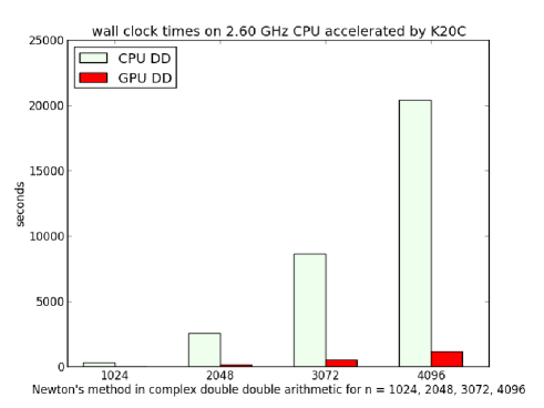
Figure 5: Figure visualizing the data of Table 3. Observe that the rightmost bar representing the accelerated run for $n=4096$ is less high than the bar for $n=2048$ without acceleration. With acceleration we can double the dimension and still obtain the results twice as fast.

Table 4 with corresponding bar plot in Figure 6 shows the timings obtained from running seven Newton iterations in real quad double arithmetic. Because of shared memory limitations, the block size could not be larger than 127 and our preliminary implementation requires the dimension to be a multiple of the block size.

For quality up, we compare the 42m41.597s in Table 3 for $n=2048$ with the 42m22.440s in Table 4 for $n=4064$. With the accelerated version we obtain twice as accurate results for almost double the dimensions in about the same time.

Table 4: Running seven iterations of Newton’s method in real quad double arithmetic on one core on the CPU and accelerated by the K20C (GPU) with block size equal to 127, with the evaluation and differentiation done by the CPU.

$n$	mode	real	user	sys	speedup
1016	CPU	14m52.539s	14m50.502s	0.511s
	GPU	59.570s	48.923s	10.377s	14.98
2032	CPU	118m20.789s	118m10.189s	0.134s
	GPU	6m42.595s	4m25.458s	2m16.315s	17.64
3048	CPU	396m08.623s	395m34.182s	0.560s
	GPU	21m21.047s	13m49.481s	7m29.744s	18.55
4064	CPU	939m16.703s	937m50.275s	0.941s
	GPU	42m22.440s	26m2.594s	16m16.286s	22.17

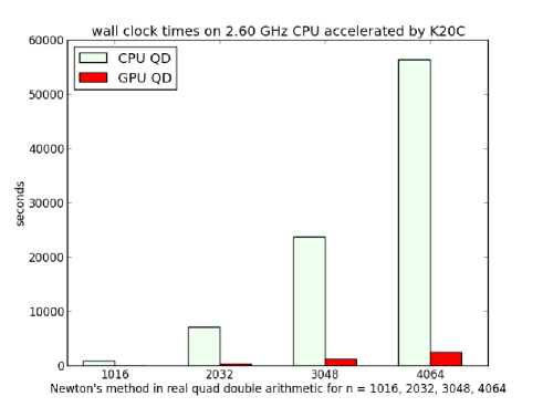
Figure 6: Figure visualizing the data of Table 4. Compared to complex double double arithmetic, we observe the timings are of the same magnitude as the cost for complex double double is similar to the cost of real quad double arithmetic. For real quad doubles, the speedups are slightly better.

5.3 the cyclic $n$-roots problem

A system relevant to operator algebras is:

$$\begin{cases}x_{0}+x_{1}+\cdots+x_{n-1}=0\\ x_{0}x_{1}+x_{1}x_{2}+\dots+x_{n-2}x_{n-1}+x_{n-1}x_{0}=0\\ i=3,4,\ldots,n-1:\displaystyle\sum_{j=0}^{n-1}~{}\prod_{k=j}^{j+i-1}x_{k~{}{\rm mod}~{}n}=0\\ x_{0}x_{1}x_{2}\cdots x_{n-1}-1=0.\\ \end{cases}$$ (7)

The system is a benchmark problem in computer algebra: [1], [7], [10], [12], [33].

Except for the last equation, every polynomial has $n$ monomials, so the total number of monomials grows as $n^{2}-n+2$. As each monomial is a product of at most $n$ variables, the total cost to evaluate and differentiate the system is $O(n^{3})$.

Table 5 contains experimental results on the evaluation of the polynomials in the cyclic $n$-roots system and the evaluation of its Jacobian matrix. For both the CPU and GPU we observe the $O(n^{3})$ cost: doubling the dimension increases the cost with a factor bounded by 8. The speedups improve for larger problems and for increased precision, see Figure 7 for a plot of the results in complex double arithmetic, using the algorithmic circuits of Figures 1 and 2. For complex double double and quad double arithmetic, the problem is no longer memory but is compute bound and the computations in the DD and QD rows of Table 5 use global instead shared memory.

Table 5: Evaluation and differentiation of the cyclic $n$-roots problem in complex double (D), complex double double (DD), and complex quad double (QD) arithmetic for increasing dimensions $n$. The times in milliseconds are obtained with the NVIDIA profiler.

	$n$		time	speedup
D	128	CPU	16.39ms
		GPU	1.13ms	14.87
	256	CPU	136.26ms
		GPU	6.97ms	19.55
	384	CPU	475.94ms
		GPU	21.59ms	22.05
	448	CPU	747.44ms
		GPU	32.68ms	22.87
	512	CPU	1097.20ms
		GPU	46.43ms	23.63
DD	128	CPU	144.27ms
		GPU	6.45ms	22.36
	256	CPU	1169.07ms
		GPU	37.15ms	31.47
	384	CPU	3981.07ms
		GPU	120.48ms	33.04
	448	CPU	6323.17ms
		GPU	182.19ms	34.52
	512	CPU	9411.55ms
		GPU	267.39ms	35.20
QD	128	CPU	1349.55ms
		GPU	29.45ms	45.82
	256	CPU	10987.87ms
		GPU	152.82ms	71.90
	384	CPU	37323.08ms
		GPU	513.78ms	72.64
	448	CPU	59247.04ms
		GPU	809.15ms	73.22

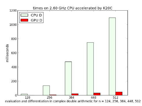
Figure 7: Figure visualizing the data for complex double arithmetic (D) of Table 5. Observe that the rightmost bar representing the accelerated run for $n=512$ is about half the size of the bar for $n=128$ without acceleration. With acceleration we can double the dimension and still obtain the results twice as fast.

We end this paper with the application of Newton’s method on the cyclic $n$-roots problem $f({\bf x})={\bf 0}$ for $n=512$. The setup is as follows. We generate a random complex vector ${\bf z}\in{\mathbb{C}}^{512}$ and consider the system $f({\bf x})-f({\bf z})t={\bf 0}$, for $t<1$. For $t=1$, we have that ${\bf z}$ is a solution and for $t$ sufficiently close to 1, Newton’s method will converge. This setup corresponds to the start in running a Newton homotopy, for $t$ going from one to zero. In complex double double arithmetic, with seven iterations Newton’s method converges to the full precision. The CPU time is 78,055.71 seconds while the GPU accelerated time is 5,930.96 seconds, reducing 21 minutes to about 1.6 minutes, giving a speedup factor of about 13.

6 Conclusions

To accurately evaluate and differentiate polynomials in several variables given in sparse distributed form we reorganized the arithmetic circuits so all threads in block can contribute to the computation. This computation is memory bound for double arithmetic and the techniques to optimize a parallel reduction are beneficial also for real double double arithmetic, but for complex double double and quad double arithmetic the problem becomes compute bound.

We illustrated our CUDA implementation on two benchmark problems in polynomial system solving. For the first problem, the cost of evaluation and differentiation grows linearly in the dimension and then the cost of linear system solving dominates. For systems with polynomials of high degree such as the cyclic $n$-roots problem, the implementation to evaluate the system and compute its Jacobian matrix achieved double digits speedups, sufficiently large enough to compensate for one extra level of precision. With GPU acceleration we obtain more accurate results faster, for larger dimensions.

References

- [1] D. Adrovic and J. Verschelde. Polyhedral methods for space curves exploiting symmetry applied to the cyclic -roots problem. In V.P. Gerdt, W. Koepf, E.W. Mayr, and E.V. Vorozhtsov, editors, Proceedings of CASC 2013, pages 10–29, 2013.
- [2] E. Agullo, C. Augonnet, J. Dongarra, M. Faverge, H. Ltaief, S. Thibault, and S. Tomov. QR factorization on a multicore node enhanced with multiple GPU accelerators. In Proceedings of the 2011 IEEE International Parallel Distributed Processing Symposium (IPDPS 2011), pages 932–943. IEEE Computer Society, 2011.
- [3] S.G. Akl. Superlinear performance in real-time parallel computation. The Journal of Supercomputing, 29(1):89–111, 2004.
- [4] M. Anderson, G. Ballard, J. Demmel, and K. Keutzer. Communication-avoiding QR decomposition for GPUs. In Proceedings of the 2011 IEEE International Parallel Distributed Processing Symposium (IPDPS 2011), pages 48–58. IEEE Computer Society, 2011.
- [5] T. Bartkewitz and T. Güneysu. Full lattice basis reduction on graphics cards. In F. Armknecht and S. Lucks, editors, WEWoRC’11 Proceedings of the 4th Western European conference on Research in Cryptology, volume 7242 of Lecture Notes in Computer Science, pages 30–44. Springer-Verlag, 2012.
- [6] C. Bischof, N. Guertler, A. Kowartz, and A. Walther. Parallel reverse mode automatic differentiation for OpenMP programs with ADOL-C. In C. Bischof, H.M. Bücker, P. Hovland, U. Naumann, and J. Utke, editors, Advances in Automatic Differentiation, pages 163–173. Springer-Verlag, 2008.
- [7] G. Björck and R. Fröberg. Methods to “divide out” certain solutions from systems of algebraic equations, applied to find all cyclic 8-roots. In M. Gyllenberg and L.E. Persson, editors, Analysis, Algebra and Computers in Math. research, volume 564 of Lecture Notes in Mathematics, pages 57–70. Dekker, 1994.
- [8] T. Brandes, A. Arnold, T. Soddemann, and D. Reith. CPU vs. GPU - performance comparison for the Gram-Schmidt algorithm. The European Physical Journal Special Topics, 210(1):73–88, 2012.
- [9] S. Collange, M. Daumas, and D. Defour. Interval arithmetic in CUDA. In Wen mei W. Hwu, editor, GPU Computing Gems Jade Edition, pages 99–107. Elsevier, 2012.
- [10] Y. Dai, S. Kim, and M. Kojima. Computing all nonsingular solutions of cyclic-n polynomial using polyhedral homotopy continuation methods. J. Comput. Appl. Math., 152(1-2):83–97, 2003.
- [11] J. Demmel, Y. Hida, X.S. Li, and E.J. Riedy. Extra-precise iterative refinement for overdetermined least squares problems. ACM Trans. Math. Softw., 35(4):28:1–28:32, 2009.
- [12] J.C. Faugère. Finding all the solutions of Cyclic 9 using Gröbner basis techniques. In Computer Mathematics - Proceedings of the Fifth Asian Symposium (ASCM 2001), volume 9 of Lecture Notes Series on Computing, pages 1–12. World Scientific, 2001.
- [13] B. Foster, S. Mahadevan, and R. Wang. A GPU-based approximate SVD algorithm. In Parallel Processing and Applied Mathematics, volume 7203 of Lecture Notes in Computer Science Volume, pages 569–578. Springer-Verlag, 2012.
- [14] G.H. Golub and C.F. Van Loan. Matrix Computations. The Johns Hopkins University Press, third edition, 1996.
- [15] L. Gonzalez-Vega. Some examples of problem solving by using the symbolic viewpoint when dealing with polynomial systems of equations. In J. Fleischer, J. Grabmeier, F.W. Hehl, and W. Küchlin, editors, Computer Algebra in Science and Engineering, pages 102–116. World Scientific, 1995.
- [16] M. Grabner, T. Pock, T. Gross, and B. Kainz. Automatic differentiation for GPU-accelerated 2D/3D registration. In C. Bischof, H.M. Bücker, P. Hovland, U. Naumann, and J. Utke, editors, Advances in Automatic Differentiation, pages 259–269. Springer-Verlag, 2008.
- [17] A. Griewank and A. Walther. Evaluating Derivatives: Principles and Techniques of Algorithmic Differentiation. SIAM, second edition, 2008.
- [18] M. Harris. Optimizing parallel reduction in CUDA. White paper available at http://docs.nvidia.com.
- [19] M. Harris. Parallel prefix sum (scan) in CUDA. White paper available at http://docs.nvidia.com.
- [20] Y. Hida, X.S. Li, and D.H. Bailey. Algorithms for quad-double precision floating point arithmetic. In 15th IEEE Symposium on Computer Arithmetic (Arith-15 2001), 11-17 June 2001, Vail, CO, USA, pages 155–162. IEEE Computer Society, 2001. Shortened version of Technical Report LBNL-46996, software at http://crd.lbl.gov/dhbailey/ mpdist.
- [21] N.J. Higham. Accuracy and Stability of Numerical Algorithms. SIAM, 1996.
- [22] C.T. Kelley. Solution of the Chandrasekhar -equation by Newton’s method. J. Math. Phys., 21(7):1625–1628, 1980.
- [23] A. Kerr, D. Campbell, and M. Richards. QR decomposition on GPUs. In D. Kaeli and M. Leeser, editors, Proceedings of 2nd Workshop on General Purpose Processing on Graphics Processing Units (GPGPU’09), pages 71–78. ACM, 2009.
- [24] D.B. Kirk and W.W. Hwu. Programming Massively Parallel Processors. A Hands-on Approach. Morgan Kaufmann/Elsevier, second edition, 2013.
- [25] R.A. Klopotek and J. Porter-Sobieraj. Solving systems of polynomial equations on a GPU. In M. Ganzha, L. Maciaszek, and M. Paprzycki, editors, Preprints of the Federated Conference on Computer Science and Information Systems, September 9-12, 2012, Wroclaw, Poland, pages 567–572, 2012.
- [26] X. Li, J. Demmel, D. Bailey, G. Henry, Y. Hida, J. Iskandar, W. Kahan, S. Kang, A. Kapur, M. Martin, B. Thompson, T. Tung, and D. Yoo. Design, implementation and testing of extended and mixed precision BLAS. ACM Trans. Math. Softw., 28(2):152–205, 2002. This is a shortened version of Technical Report LBNL-45991.
- [27] M. Lu, B. He, and Q. Luo. Supporting extended precision on graphics processors. In A. Ailamaki and P.A. Boncz, editors, Proceedings of the Sixth International Workshop on Data Management on New Hardware (DaMoN 2010), June 7, 2010, Indianapolis, Indiana, pages 19–26, 2010. Software at http://code.google.com/p/gpuprec/.
- [28] Y. Luo and R. Duraiswami. Efficient parallel nonnegative least squares on multicore architectures. SIAM J. Sci. Comp., 33(5):2848–2863, 2011.
- [29] M.M. Maza and W. Pan. Solving bivariate polynomial systems on a GPU. ACM Communications in Computer Algebra, 45(2):127–128, 2011.
- [30] J.J. Moré. A collection of nonlinear model problems. In Computational Solution of Nonlinear Systems of Equations, volume 26 of Lectures in Applied Mathematics, pages 723–762. AMS, 1990.
- [31] D. Mukunoki and D. Takashashi. Implementation and evaluation of triple precision BLAS subroutines on GPUs. In Proceedings of the 2012 IEEE 26th International Parallel and Distributed Processing Symposium Workshops. 21-25 May 2012, Shanghai China, pages 1372–1380. IEEE Computer Society, 2012.
- [32] S.M. Rump. Verification methods: Rigorous results using floating-point arithmetic. Acta Numerica, 19:287–449, 2010.
- [33] R. Sabeti. Numerical-symbolic exact irreducible decomposition of cyclic-12. LMS Journal of Computation and Mathematics, 14:155–172, 2011.
- [34] J. Utke, L. Hascoët, P. Heimbach, C. Hill, P. Hovland, and U. Naumann. Toward ajoinable MPI. In Proceedings of the 10th IEEE International Workshop on Parallel and Distributed Scientific and Engineering Computing (PDSEC 2009), pages 1–8, 2009.
- [35] J. Verschelde. Algorithm 795: PHCpack: A general-purpose solver for polynomial systems by homotopy continuation. ACM Trans. Math. Softw., 25(2):251–276, 1999.
- [36] J. Verschelde and G. Yoffe. Polynomial homotopies on multicore workstations. In M.M. Maza and J.-L. Roch, editors, Proceedings of the 4th International Workshop on Parallel Symbolic Computation (PASCO 2010), July 21-23 2010, Grenoble, France, pages 131–140. ACM, 2010.
- [37] J. Verschelde and G. Yoffe. Evaluating polynomials in several variables and their derivatives on a GPU computing processor. In Proceedings of the 2012 IEEE 26th International Parallel and Distributed Processing Symposium Workshops (PDSEC 2012), pages 1391–1399. IEEE Computer Society, 2012.
- [38] J. Verschelde and G. Yoffe. Orthogonalization on a general purpose graphics processing unit with double double and quad double arithmetic. In Proceedings of the 2013 IEEE 27th International Parallel and Distributed Processing Symposium Workshops (PDSEC 2013), pages 1373–1380. IEEE Computer Society, 2013.
- [39] V. Volkov and J. Demmel. Benchmarking GPUs to tune dense linear algebra. In Proceedings of the 2008 ACM/IEEE conference on Supercomputing. IEEE Press, 2008. Article No. 31.