A comprehensive analysis of the geometry of
TDOA maps in localisation problems

Abstract

In this manuscript we consider the well-established problem of TDOA-based source localization and propose a comprehensive analysis of its solutions for arbitrary sensor measurements and placements. More specifically, we define the TDOA map from the physical space of source locations to the space of range measurements (TDOAs), in the specific case of three receivers in 2D space. We then study the identifiability of the model, giving a complete analytical characterization of the image of this map and its invertibility. This analysis has been conducted in a completely mathematical fashion, using many different tools which make it valid for every sensor configuration. These results are the first step towards the solution of more general problems involving, for example, a larger number of sensors, uncertainty in their placement, or lack of synchronization.

, , ,

1 Introduction

The localization of radiant sources based on a spatial distribution of sensors has been an important research topic for the past two decades, particularly in the area of space-time audio processing. Among the many solutions that are available in the literature, those based on Time Differences Of Arrival (TDOAs) between distinct sensors of a signal emitted by the source are the most widespread and popular. Such solutions, in fact, are characterized by a certain flexibility, a reasonably modest computational cost with respect to other solutions and a certain robustness against noise. Popular TDOA-based solutions are [10, 2, 24, 26, 27, 31, 32, 33, 41, 44, 46, 48, 49, 52, 54, 55, 7].

Let us consider the problem of planar source localization in a homogeneous medium with negligible reverberation. From elementary geometry, the locus of putative source locations that are compatible with a TDOA measurement between two sensors in positions $\mathbf{m}_{i}$ and $\mathbf{m}_{j}$ is one branch of a hyperbola of foci $\mathbf{m}_{i}$ and $\mathbf{m}_{j}$, whose aperture depends on the range difference (TDOA $\times$ speed of sound). A single TDOA measurement is, therefore, not sufficient for localizing a source, but it narrows down the set of locations that are compatible with that measurement by reducing its dimensionality.

Multiple measurements do enable localization but measurement errors cause the corresponding hyperbola branches not to meet at a single point, thus ruling out simple geometric intersection as a solution to the localization problem [14]. This is why research has focused on techniques that are aimed at overcoming this problem while achieving robustness. Examples are Maximum Likelihood (ML) [16, 26, 53]; Least Squares (LS) [2]; and Constrained Least Squares (CLS) [34, 48], which offer accurate results for the most common configurations of sensors.

There are many situations, however, in which it is necessary to minimize the number of sensors in use, due to specific sensor placement constraints, or cost limitations. In these cases it becomes important to assess how the solutions to the localization problem “behave” (and how many there are) as the measurements or the sensor geometry vary. This problem has been partially addressed in the case of the localization of a radio-beacon receiver in LORAN navigation systems [49] and in the context of the Global Positioning System (GPS), where measurements are of Time Of Arrivals (TOAs) instead of TDOAs (see [9, 37, 1, 15, 38, 30, 28, 8, 18, 19]). In particular, these studies provide the solution for the case of planar (2D) source localization with three receivers (i.e. with two TDOAs) and they recognize the possibility of dual solutions in some instances, as two different source positions could correspond to the same pair of TDOA measurements.

Recently, in [51] the author focused on the assessment of the ill-posedness of the localization problem in the case of 2D minimal sensor configurations, i.e. on quantify how changes in the measurements propagate onto changes in the estimated source location. In particular, in the same quoted manuscript it has been introduced the space of TDOA measurements and it has been shown that in this space there exist small regions associated with dual solutions corresponding to large regions in physical space. This assessment, however, is performed in a simulative fashion and for one specific sensor geometry, and it would be important to extend its generality further.

What we propose in this manuscript is a generalization of the discussion contained in [51] based on a fully analytical and mathematically rigorous approach. We encode the TDOA localization problem into a map, called the TDOA map, from the space of source locations to the space of TDOA measurements and we offer a complete characterization of such a map. Not only it is our goal to analytically derive results shown in [51] (irrespective of the geometry of the acquisition system), but also to complete the characterization of the TDOA map by analyzing the properties of its image and pre-image, finding closed-form expressions for the boundaries of the regions of interest. We observe that this approach to the problem fits into the research field of structural identifiability of complex systems (see for example [11, 40]), where one is interested in studying if the parameters of a model (in our case, the coordinates of the source) can be fully retrieved from the experimental data. A similar analysis of the source localization problem has been proposed and investigated very recently also in [5, 17], the latter in the context of the TOA–based target tracking.

We believe that characterizing the TDOA map to its fullest extent, even in the simplest case of three calibrated and synchronous sensors, is a necessary step for developing new mathematical tools for a wide range of more general problems. One immediate consequence of this gained knowledge is the possibility to study how to optimize sensor placement in terms of robustness against noise or measuring errors. More importantly, this study paves the way to new venues of research. For example, it enables the statistical analysis of error propagation in TDOA-based localization problems; and it allows us to approach more complex scenarios where the uncertainty lies with sensor synchronization or spatial sensor placement. This prospective investigation, in fact, is in line with the recently revamped interest of the research community in self-calibrating and self-synchronizing spatial distributions of sensors [16, 45, 47].

Our analysis starts from [20], where a different perspective on the localization problem is offered through the adoption of the Space–Range Differences (SRD) reference frame, where the wavefront propagation is described by a (propagation) cone whose vertex lies on the source location. As range difference measurements (TDOA $\times$ propagation speed) are bound to lie on the surface of the propagation cone, localizing a source in the SRD space corresponds to finding the vertex of the cone that best fits the measured data. The SRD reference frame is also used in [12] to offer geometric interpretations to the underlying principles behind the most common TDOA-based localization solutions. Although not explicitly claimed, the localization problem is described in [20, 12] in terms of null surfaces and planes in the 3D Minkowski space. This suggests us that exterior algebra can give us powerful tools for approaching our problem as well. We therefore begin our analysis by showing how the SRD reference frame can be better represented within the framework of exterior algebra, and we show how the newly gained tools allow us to derive a global analytical characterization of the TDOA map. Working with exterior algebra in the Minkowski space is not unheard of in the literature of space-time signal processing. In [18, 19], for example, this representation is used for approaching source localization in the GPS context.

The manuscript is organized as shown in Fig. 1. Section 2 introduces the concept of TDOA map. Two are the TDOA maps defined: $\boldsymbol{\tau_{2}}$, where the TDOAs are referred to a common reference microphone; and $\boldsymbol{\tau_{2}^{*}}$, which considers the TDOAs between all the pairs of microphones. The two maps are, in fact, equivalent in absence of measurement errors. This is why most of the techniques in the literature work with $\boldsymbol{\tau_{2}}$. However, in the presence of measurement noise, adopting $\boldsymbol{\tau_{2}^{*}}$ helps gain robustness. For this reason we decided to consider both $\boldsymbol{\tau_{2}}$ and $\boldsymbol{\tau_{2}^{*}}.$ In order to introduce our mathematical formalisms with some progression, in the first part of the manuscript our analysis will concern $\boldsymbol{\tau_{2}}$. Section 3 focuses on the local analysis of the TDOA map $\boldsymbol{\tau_{2}}$. In practice, we show what can be accomplished using “conventional” analysis tools (analysis of the Jacobian matrix). This analysis represents the first step towards the study of the invertibility of $\boldsymbol{\tau_{2}}$. In Section 4 we move forward with our representation by defining the TDOA mapping in the Space - Range Difference (SRD) reference frame. This is where we show that the Minkowski space is the most natural representation for a mapping that “lives” in the SRD reference frame. Section 5 describes the early properties of $\boldsymbol{\tau_{2}}$, with particular emphasis on the fact that its image is contained in a compact polygonal region. Section 6 offers a complete description of the mapping $\boldsymbol{\tau_{2}}$ for the case of non-aligned microphones. In particular, Subsection 6.1 shows that the preimage (inverse image) of $\boldsymbol{\tau_{2}}$ can be described in terms of the non-negative roots of a degree-2 equation, while 6.3 describes $\mathrm{Im}(\boldsymbol{\tau})$ and the cardinality of the pre-image. Finally, Subsection 6.4 shows the pre-image regions in $\boldsymbol{\tau_{2}}$ and the bifurcation curve $\tilde{E}$ that divides the region of cardinality 1 from the regions of cardinality 0 or 2. Similar results are derived for the case of aligned microphones in Section 7. In Section 8 we use the previous results on $\boldsymbol{\tau_{2}}$ to describes the image and the preimages of the map $\boldsymbol{\tau^{*}_{2}}$. Section 9 discusses the impact of this work and offers an example aimed at showing that the global analysis on $\boldsymbol{\tau_{2}}$ (or $\boldsymbol{\tau_{2}^{*}}$) gives new insight on the localization problem, which could not be derived with a local approach. Finally, Section 10 draws some conclusions and describes possible future research directions that can take advantage of the analysis presented in this manuscript.

In order to keep the manuscript as self-contained as possible, in Appendix A we give an overview on exterior algebra on a vector space. For similar reasons, we also included an introduction to plane algebraic geometry in Appendix B. These two Sections, of course, can be skipped by the readers who are already familiar with these topics. Finally, in Appendix C we included the code for computing the cartesian equation of the bifurcation curve $\tilde{E}$.

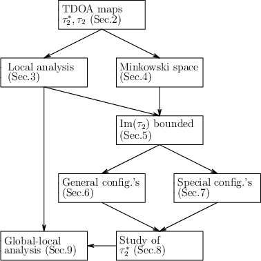
Figure 1: Organization of the manuscript.

2 From the physical model to its mathematical description

As mentioned above, we focus on the case of coplanar source and receivers, with synchronized receivers in known locations and with anechoic and homogenous propagation. The physical world can therefore be identified with the Euclidean plane, here referred to as the $x$–plane. This choice [20, 12] allows us to approach the problem with more progression and visualization effectiveness.

After choosing an orthogonal Cartesian co-ordinate system, the Euclidean $x$–plane can be identified with $\mathbb{R}^{2}$. On this plane, $\mathbf{m_{i}}=(x_{i},y_{i}),\ i=0,1,2$ are the positions of the microphones and $\mathbf{x}=(x,y)$ is the position of the source $S$. The corresponding displacement vectors are

$$\mathbf{d_{i}}(\mathbf{x})=\mathbf{x}-\mathbf{m_{i}},\qquad\mathbf{d_{ji}}=\mathbf{m_{j}}-\mathbf{m_{i}},\qquad i,j=0,1,2,$$ (1)

whose moduli are $d_{i}(\mathbf{x})$ and $d_{ji}$, respectively. Generally speaking, given a vector $\mathbf{v}$, we denote its norm $||\mathbf{v}||$ with $v$ and with $\tilde{\mathbf{v}}=\frac{\mathbf{v}}{v}$ the corresponding unit vector.

Without loss of generality, we assume the speed of propagation in the medium to be equal to $1$. For each pair of different microphones, the measured TDOA $\hat{\tau}_{ji}(\mathbf{x})$ turns out to be equal to the pseudorange (i.e. the range difference)

$${\tau}_{ji}(\mathbf{x})=d_{j}(\mathbf{x})-d_{i}(\mathbf{x}),\quad i,j=0,1,2,$$ (2)

plus a measurement error $\epsilon_{ji}:$

$$\hat{\tau}_{ji}(\mathbf{x})=\tau_{ji}(\mathbf{x})+\epsilon_{ji},\quad i,j=0,1,2.$$ (3)

A wavefront originating from a source in $\mathbf{x}$ will produce a set of measurements $(\hat{\tau}_{10}(\mathbf{x}),\hat{\tau}_{20}(\mathbf{x}),\hat{\tau}_{21}(\mathbf{x}))$. As the measurement noise is a random variable, we are concerning with a stochastic model.

Definition 2.1

The complete TDOA model is

$$\boldsymbol{\hat{\tau}_{2}^{*}}(\mathbf{x})=(\hat{\tau}_{10}(\mathbf{x}),\hat{\tau}_{20}(\mathbf{x}),\hat{\tau}_{21}(\mathbf{x})).$$ (4)

The deterministic part of this model is obtained by setting $\epsilon_{ji}=0$ in $\boldsymbol{\hat{\tau}_{2}^{*}}(\mathbf{x})$, which gives us the complete TDOA map:

$$\begin{array}[]{cccc}\boldsymbol{\tau_{2}^{*}}:&\mathbb{R}^{2}&\to&\mathbb{R}^{3}\\ &\mathbf{x}&\to&(\tau_{10}(\mathbf{x}),\tau_{20}(\mathbf{x}),\tau_{21}(\mathbf{x})).\end{array}$$ (5)

The target set is referred to as the $\tau^{*}$–space.

In this manuscript we approach the deterministic problem, therefore we only consider the complete TDOA map. Using the above definition, localization problems can be readily formulated in terms of $\boldsymbol{\tau_{2}^{*}}.$ For example, given a set of measurements, we are interested to know if there exists a source that has produced them, if such a source is unique, and where it is. In a mathematical setting, these questions are equivalent to:

• given $\boldsymbol{\tau_{2}^{*}}\in\mathbb{R}^{3},$ does there exist a source in the $x$–plane such that $\boldsymbol{\tau_{2}^{*}}(\mathbf{x})=\boldsymbol{\tau^{*}}$, i.e. $\boldsymbol{\tau^{*}}\in\mbox{Im}(\boldsymbol{\tau_{2}^{*}})$?

• If $\mathbf{x}$ exists, is it unique, i.e. $|\boldsymbol{\tau_{2}^{*}}^{-1}(\boldsymbol{\tau})|=1$?

• If so, is it possible to find the coordinates of $\mathbf{x}$? i.e. given $\boldsymbol{\tau^{*}}$, can we find the only $\mathbf{x}$ that solves the equation $\boldsymbol{\tau_{2}^{*}}(\mathbf{x})=\boldsymbol{\tau^{*}}$?

With these problems in mind, we focus on the study of the image of the TDOA map $\boldsymbol{\tau_{2}^{*}}$ and of its global properties. In particular, we are interested in finding the locus of points where the map becomes $1$–to–$1$. Moreover, as solving the localization problem consists of finding the inverse image of $\boldsymbol{\tau^{*}}\in\mbox{Im}(\boldsymbol{\tau_{2}^{*}})$, we aim at giving an explicit description of the preimages, also called the fibers, of $\boldsymbol{\tau_{2}^{*}}$.

The complete model $\boldsymbol{\hat{\tau}_{2}^{*}}(\mathbf{x})$ takes into account each one of the three TDOA that can be defined between the sensors. This, in fact, becomes necessary when working in a realistic (noisy) situation [50]. We should keep in mind, however, that there is a linear relationship between the pseudoranges (3), which allows us to simplify the deterministic problem.

Definition 2.2

Let $(\tau_{10},\tau_{20},\tau_{21})$ be the coordinates of the $\tau^{*}$–space. Then, $\mathcal{H}$ is the plane of equation $\tau_{10}-\tau_{20}+\tau_{21}=0$.

Lemma 2.3

The image $\mbox{Im}(\boldsymbol{\tau}_{2}^{*})$ is contained in $\mathcal{H}$.

Proof. For each $\mathbf{x}\in\mathbb{R}^{2}$ we have

$$\tau_{10}(\mathbf{x})-\tau_{20}(\mathbf{x})+\tau_{21}(\mathbf{x})=0$$ (6)

from the definition (2) of pseudoranges. $\square$

In the literature, Lemma 2.3 is usually presented by saying that there are only two linearly independent pseudoranges and $(\tau_{10}(\mathbf{x}),\tau_{20}(\mathbf{x}))$, for example, are sufficient for completely encoding the deterministic TDOA model. This suggests us to define a reduced version of the above definition:

Definition 2.4

The map from the position of the source in the $x$-plane to the linearly independent pseudoranges

$$\begin{array}[]{cccc}\boldsymbol{\tau_{2}}:&\mathbb{R}^{2}&\longrightarrow&\mathbb{R}^{2}\\ &\mathbf{x}&\longrightarrow&\quad(\tau_{10}(\mathbf{x}),\tau_{20}(\mathbf{x}))\end{array}$$ (7)

is called the TDOA map. The target set is referred to as the $\tau$–plane.

In $\boldsymbol{\tau_{2}}$ we consider only the pseudoranges involving receiver $\mathbf{m_{0}}$, which we call reference microphone. If $p_{i}:\mathcal{H}\to\mathbb{R}^{2}$ is the projection that takes care of forgetting the $i$–th coordinate, we have that $\boldsymbol{\tau_{2}^{*}}$ is related to $\boldsymbol{\tau_{2}}$ by $\boldsymbol{\tau_{2}}=p_{3}\circ\boldsymbol{\tau_{2}^{*}}$. As $p_{i}$ is clearly $1$–to–$1$, it follows that all the previous questions about the deterministic localization problem can be equivalently formulated in terms of $\boldsymbol{\tau_{2}}$ and its image Im($\boldsymbol{\tau_{2}}$) (see Figure 12 in Section 8 for an example of Im($\boldsymbol{\tau_{2}^{*}}$) and its projection Im($\boldsymbol{\tau_{2}}$) via $p_{3}$). Analogous considerations can be done if we consider $p_{1}\circ\boldsymbol{\tau_{2}^{*}}$ or $p_{2}\circ\boldsymbol{\tau_{2}^{*}}$, that is equivalent to choose $\mathbf{m_{2}}$ or $\mathbf{m_{1}}$ as reference point, respectively.

In Sections from 3 to 7, we will focus on the study of $\boldsymbol{\tau_{2}}$ and we will complete the analysis of $\boldsymbol{\tau_{2}^{*}}$ in Section 8. For reasons of notational simplicity, when we study the map $\boldsymbol{\tau_{2}}$ we will drop the second subscript and simply write $\tau_{h}(\mathbf{x})=\tau_{h0}(\mathbf{x})$, $h=1,2$. Moreover, as we focus on the deterministic model, in the rest of the manuscript we will interchangeably use the terms pseudorange and TDOA.

3 Local analysis of $\boldsymbol{\tau_{2}}$

In this Section, we present a local analysis of the TDOA map $\boldsymbol{\tau_{2}}$. From a mathematical standpoint, this is the first natural step towards studying of the invertibility of $\boldsymbol{\tau_{2}}$. In fact, as stated by the Inverse Function Theorem, if the Jacobian matrix $J(\mathbf{x})$ of $\boldsymbol{\tau_{2}}$ is invertible in $\mathbf{x}$, then $\boldsymbol{\tau_{2}}$ is invertible in a neighborhood of $\mathbf{x}$. Studying the invertibility of a map through linearization (i.e. studying its Jacobian matrix) is a classical choice when investigating the properties of a complex (non–linear) model. In the case of acoustic source localization, for example, [45, 20] adopt this method to study the accuracy of various statistical estimators for the TDOA model. As a byproduct of our study, at the end of the section we will discuss how the accuracy in a noisy scenario is strictly related to the existence of the so-called degeneracy locus, which is the locus where the rank of $J(\mathbf{x})$ drops.

The component functions $\tau_{i}(\mathbf{x})$ of $\boldsymbol{\tau_{2}}$ are differentiable in $\mathbb{R}^{2}\setminus\{\mathbf{m_{0}},\mathbf{m_{1}},\mathbf{m_{2}}\}$, therefore so is $\boldsymbol{\tau_{2}}.$ The $i$–th row of $J(\mathbf{x})$ is the gradient $\nabla\tau_{i}(\mathbf{x})$, i.e.

$$\qquad\qquad\nabla\tau_{i}(\mathbf{x})=\left(\frac{x-x_{i}}{d_{i}(\mathbf{x})}-\frac{x-x_{0}}{d_{0}(\mathbf{x})}\;,\;\frac{y-y_{i}}{d_{i}(\mathbf{x})}-\frac{y-y_{0}}{d_{0}(\mathbf{x})}\right)=\mathbf{\tilde{d}_{i}}(\mathbf{x})-\mathbf{\tilde{d}_{0}}(\mathbf{x}).$$ (8)

Definition 3.1

Let us assume that $\mathbf{m_{0}},\mathbf{m_{1}},\mathbf{m_{2}}$ are not collinear. Let $r_{0},r_{1},r_{2}$ be the lines that pass through two of such three points, in compliance with the notation $\mathbf{m_{i}}\notin r_{i}$, $i=0,1,2$. Let us split each line in three parts as $r_{0}=r_{0}^{-}\cup r_{0}^{0}\cup r_{0}^{+}$, where $r_{0}^{0}$ is the segment with endpoints $\mathbf{m_{1}}$ and $\mathbf{m_{2}}$, $r_{0}^{-}$ is the half–line originating from $\mathbf{m_{2}}$ and not containing $\mathbf{m_{1}}$, and $r_{0}^{+}$ is the half–line originating from $\mathbf{m_{1}}$ and not containing $\mathbf{m_{2}}$. Similar splittings are done for $r_{1},r_{2}$, with $r_{1}^{+},r_{2}^{+}$ having $\mathbf{m_{0}}$ as endpoint.

Let us now assume that $\mathbf{m_{0}},\mathbf{m_{1}},\mathbf{m_{2}}$ belong to the line $r$. Then, $r^{0}$ is the smallest segment containing all three points and $r^{c}$ is its complement in $r$.

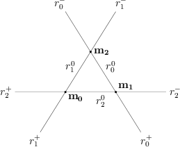
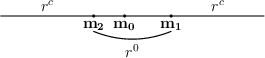
Figure 2: A general and a collinear configuration of the microphones $\mathbf{m}_{i},\;i=0,1,2$. Left-hand side: line $r_{i}^{+},\;r_{i}^{-}$ and $r_{i}^{0}$ refer to the portions of the line joining the microphones $j$ and $k,\;j,k\neq i$.

Theorem 3.2

Let $J(\mathbf{x})$ be the Jacobian matrix of $\boldsymbol{\tau_{2}}$ at $\mathbf{x}\not=\mathbf{m_{0}},\mathbf{m_{1}},\mathbf{m_{2}}.$ Then,

1. if $\mathbf{m_{0}},\mathbf{m_{1}},\mathbf{m_{2}}$ are not collinear, then

   $${\rm rank}(J(\mathbf{x}))=\left\{\begin{array}[]{cl}1&\mbox{if }\mathbf{x}\in\left(\cup_{i=0}^{2}(r_{i}^{-}\cup r_{i}^{+})\right),\\ 2&\mbox{otherwise};\end{array}\right.$$

2. if $\mathbf{m_{0}},\mathbf{m_{1}},\mathbf{m_{2}}$ are collinear, then

   $${\rm rank}(J(\mathbf{x}))=\left\{\begin{array}[]{cl}0&\mbox{if }\mathbf{x}\in r^{c},\\ 1&\mbox{if }\mathbf{x}\in r^{0},\\ 2&\mbox{otherwise.}\end{array}\right.$$

Proof. Assume $\mathbf{x}\not=\mathbf{m_{i}},$ for $i=0,1,2.$ As explained in Section 2, the $x$–plane is equipped with the Euclidean inner product, therefore we can use the machinery of Appendix A. As claimed in Proposition A.3, $\ast(\det(J(\mathbf{x})))=\nabla\tau_{1}(\mathbf{x})\wedge\nabla\tau_{2}(\mathbf{x})$. Hence, we work in the exterior algebra of the $2$–forms. From eq. (8) and the general properties of $2$–forms, we obtain

$$\eqalign{\nabla\tau_{1}(\mathbf{x})\wedge\nabla\tau_{2}(\mathbf{x})=(\mathbf{\tilde{d}_{1}}(\mathbf{x})-\mathbf{\tilde{d}_{0}}(\mathbf{x}))\wedge(\mathbf{\tilde{d}_{2}}(\mathbf{x})-\mathbf{\tilde{d}_{0}}(\mathbf{x}))=\cr=\mathbf{\tilde{d}_{1}}(\mathbf{x})\wedge\mathbf{\tilde{d}_{2}}(\mathbf{x})-\mathbf{\tilde{d}_{0}}(\mathbf{x})\wedge\mathbf{\tilde{d}_{2}}(\mathbf{x})-\mathbf{\tilde{d}_{1}}(\mathbf{x})\wedge\mathbf{\tilde{d}_{0}}(\mathbf{x}).}$$ (9)

Let us first assume that $\mathbf{\tilde{d}_{1}}(\mathbf{x}),\mathbf{\tilde{d}_{2}}(\mathbf{x})$ are linearly independent or, equivalently, that $\mathbf{x}\notin r_{0}.$ In this case there exist $a_{1},a_{2}\in\mathbb{R}$ such that

$$\mathbf{\tilde{d}_{0}}(\mathbf{x})=a_{1}\mathbf{\tilde{d}_{1}}(\mathbf{x})+a_{2}\mathbf{\tilde{d}_{2}}(\mathbf{x}).$$

After simplifying equation (9), we get

$$\det(J(\mathbf{x}))=\nabla\tau_{1}(\mathbf{x})\wedge\nabla\tau_{2}(\mathbf{x})=(-a_{1}-a_{2}+1)\,\mathbf{\tilde{d}_{1}}(\mathbf{x})\wedge\mathbf{\tilde{d}_{2}}(\mathbf{x}),$$ (10)

therefore $\det(J(\mathbf{x}))=0$ if, and only if, $a_{1}+a_{2}=1$, because the linear independence of $\mathbf{\tilde{d}_{1}}(\mathbf{x}),\mathbf{\tilde{d}_{2}}(\mathbf{x})$ implies $\mathbf{\tilde{d}_{1}}(\mathbf{x})\wedge\mathbf{\tilde{d}_{2}}(\mathbf{x})\not=0$. Furthermore, from $\mathbf{\tilde{d}_{0}}(\mathbf{x})=a_{1}\mathbf{\tilde{d}_{1}}(\mathbf{x})+a_{2}\mathbf{\tilde{d}_{2}}(\mathbf{x}),$ we obtain

$$1=\|\mathbf{\tilde{d}_{0}}(\mathbf{x})\|^{2}=a^{2}_{1}+a^{2}_{2}+2a_{1}a_{2}\mathbf{\tilde{d}_{1}}(\mathbf{x})\cdot\mathbf{\tilde{d}_{2}}(\mathbf{x}).$$

After simple calculations, the previous equality becomes

$$2a_{1}a_{2}(\mathbf{\tilde{d}_{1}}(\mathbf{x})\cdot\mathbf{\tilde{d}_{2}}(\mathbf{x})-1)=0\;,$$

therefore either $a_{1}=0$ or $a_{2}=0,$ because the third factor is different from zero. If $a_{1}=0$, then $a_{2}=1$ and $\mathbf{\tilde{d}_{0}}(\mathbf{x})=\mathbf{\tilde{d}_{2}}(\mathbf{x})$, i.e. $\mathbf{x}\in r_{1}^{+}\cup r_{1}^{-}.$ Otherwise, if $a_{2}=0$, then $a_{2}=1$ and $\mathbf{\tilde{d}_{0}}(\mathbf{x})=\mathbf{\tilde{d}_{1}}(\mathbf{x}),$ i.e. $\mathbf{x}\in r_{2}^{+}\cup r_{2}^{-}.$

On the other hand, if $\mathbf{x}\in r_{0},$ then $\mathbf{\tilde{d}_{1}}(\mathbf{x})=\mathbf{\tilde{d}_{2}}(\mathbf{x})$ if $\mathbf{x}\in r_{0}^{+}\cup r_{0}^{-},$ and $\mathbf{\tilde{d}_{1}}(\mathbf{x})=-\mathbf{\tilde{d}_{2}}(\mathbf{x})$ if $\mathbf{x}\in r_{0}^{0}.$ Therefore, the equality (9) becomes

$$\nabla\tau_{1}(\mathbf{x})\wedge\nabla\tau_{2}(\mathbf{x})=\left\{\begin{array}[]{cl}0&\mbox{ if }\mathbf{x}\in r_{0}^{+}\cup r_{0}^{-},\\ -2\mathbf{\tilde{d}_{0}}(\mathbf{x})\wedge\mathbf{\tilde{d}_{2}}(\mathbf{x})&\mbox{ if }\mathbf{x}\in r_{0}^{0}.\end{array}\right.$$

In conclusion, if $\mathbf{m_{0}},\mathbf{m_{1}},\mathbf{m_{2}}$ are not collinear, then $\det(J(\mathbf{x}))=0$ for each $\mathbf{x}\in\cup_{i=0}^{2}(r_{i}^{+}\cup r_{i}^{-}),$ proving the first claim. If, on the other hand, $\mathbf{m_{0}},\mathbf{m_{1}},\mathbf{m_{2}}$ lie on the line $r$, then $\det(J(\mathbf{x}))=0$ for all $\mathbf{x}\in r$. Furthermore, $\mathbf{\tilde{d}_{0}}(\mathbf{x})=\mathbf{\tilde{d}_{1}}(\mathbf{x})=\mathbf{\tilde{d}_{2}}(\mathbf{x})$ if and only if $\mathbf{x}\in r^{c}$, therefore $\nabla\tau_{1}(\mathbf{x})=\nabla\tau_{2}(\mathbf{x})=(0,0),$ i.e. $J(\mathbf{x})$ is the null matrix. $\square$

Theorem 3.2 has an interesting geometric interpretation.

Definition 3.3

Let $\tau\in\mathbb{R}$. The set

$$A_{i}(\tau)=\{\mathbf{x}\in\mathbb{R}^{2}|\,\tau_{i}(\mathbf{x})=\tau\}$$ (11)

is the level set of $\tau_{i}(\mathbf{x})$ in the $x$–plane.

Lemma 3.4

If $|\tau|>d_{i0},$ then $A_{i}(\tau)=\emptyset.$ Moreover, if $0<|\tau|<d_{i0},$ then $A_{i}(\tau)$ is the branch of hyperbola with foci $\mathbf{m_{0}},\mathbf{m_{i}}$ and parameter $\tau,$ while

$$A_{i}(\tau)=\cases{r_{j}^{+}&if $\tau=d_{i0}$,\\ r_{j}^{-}&if $\tau=-d_{i0}$,\\ a_{j}&if $\tau=0$,\\ }$$

where $j\not=i,\{i,j\}=\{1,2\},$ and $a_{j}$ is the line that bisects the line segment $r_{j}^{0}.$

Proof. By definition, we have $\tau_{i}(\mathbf{x})=d_{i}(\mathbf{x})-d_{0}(\mathbf{x})$, therefore the first claim follows from the classical inequalities between the sides of the triangle of vertices $\mathbf{x},\mathbf{m_{i}},\mathbf{m_{0}}$. The second claim follows from a classical result: given any hyperbola with foci $\mathbf{m_{i}},\mathbf{m_{0}}$ and parameter $c\in\mathbb{R}^{+},$ the two branches are defined by either one of the two equations

$$d_{i}(\mathbf{x})-d_{0}(\mathbf{x})=c\qquad\mbox{ and }\qquad d_{i}(\mathbf{x})-d_{0}(\mathbf{x})=-c\quad.$$

The last claim is a straightforward computation. $\square$

Fig. 3(a) shows the hyperbola branches with foci $\mathbf{m_{0}},\mathbf{m_{i}}$. By definition of level set, each point in the domain of $\tau_{i}$ lies on exactly one branch $A_{i}(\tau)$ for some $\tau\in[-d_{i0},d_{i0}]$ (by abuse of notation, we consider $A_{i}(0),A_{i}(\pm d_{i0})$ as branches of hyperbolas as well). This means that, given $\boldsymbol{\tau}=(\tau_{1},\tau_{2})$, the source is identified as the intersection points $A_{1}(\tau_{1})\cap A_{2}(\tau_{2})$. As a direct consequence, the quality of the localization depends on the type of intersection: in a noisy scenario, an error on the measurements $\boldsymbol{\tau}$ changes the shape of the related hyperbolas, therefore the localization accuracy is strictly related to the incidence angle between the hyperbolas branches (see [12] for a similar analysis of the localization problem).

Notation: We denote the tangent line to a curve $C$ at a smooth point $\mathbf{x}\in C$ as $T_{\mathbf{x},C}$.

Remark 3.5

$(1)$ $\nabla\tau_{i}(\mathbf{x})=\mathbf{0}$ if, and only if, $\mathbf{x}\in r_{j}^{+}\cup r_{j}^{-},$ with $j\not=0,i.$ In fact, $\nabla\tau_{i}(\mathbf{x})=\mathbf{0}$ is equivalent to $\mathbf{\tilde{d_{i}}(x)}=\mathbf{\tilde{d_{0}}(x)},$ i.e. $\mathbf{x}\in r_{j}^{+}\cup r_{j}^{-}$. Hence $A_{i}(\pm d_{i0})$ is nowhere smooth.

$(2)$ Assume that $\mathbf{x}\notin r_{j}^{+}\cup r_{j}^{-}$. Then, it is well-known that $\nabla\tau_{i}(\mathbf{x})$ is orthogonal to the line $T_{\mathbf{x},A_{i}(\tau_{i})}$ and that it bisects the angle $\widehat{\mathbf{m_{0}}\mathbf{x}\mathbf{m_{i}}}$, where $\mathbf{m_{0}},\mathbf{m_{i}}$ are the foci of the hyperbola. Consequently, the tangent line is parallel to the vector $\mathbf{\tilde{d}_{i}(x)+\tilde{d}_{0}(x)}$ and, quite clearly, $\nabla\tau_{i}(\mathbf{x})=\mathbf{\tilde{d}_{i}(x)-\tilde{d}_{0}(x)}$ is orthogonal to the previous vector (as we can see in Fig. 3(b), if we draw the unit vectors $\mathbf{\tilde{d_{i}}}(\mathbf{x})$ and $\mathbf{\tilde{d_{0}}}(\mathbf{x})$, their sum lies on the tangent line $T_{\mathbf{x},A_{i}(\tau_{i})}$ while their difference is the gradient $\nabla\tau_{i}(\mathbf{x})$).

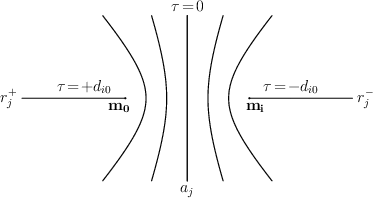
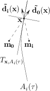
a                  $(a)$                                                $(b)$

Figure 3: $(a)$ Level sets $A_{i}(\tau)$; $(b)$ Gradient and tangent line $T_{\mathbf{x},A_{i}(\tau)}$.

Proposition 3.6

Let $\mathbf{x}\in A_{1}(\tau_{1})\cap A_{2}(\tau_{2}).$ Then,

1. if $\mathbf{m_{0}},\mathbf{m_{1}},\mathbf{m_{2}}$ are not collinear, then $T_{\mathbf{x},A_{1}(\tau_{1})}\not=T_{\mathbf{x},A_{2}(\tau_{2})},$ or equivalently, $A_{1}(\tau_{1})$ and $A_{2}(\tau_{2})$ meet transversally at $\mathbf{x}$ if, and only if, $\mathbf{x}\in\mathbb{R}^{2}\setminus\{\cup_{i=0}^{2}(r_{i}^{+}\cup r_{i}^{-})\};$

2. if $\mathbf{m_{0}},\mathbf{m_{1}},\mathbf{m_{2}}$ lie on $r$, then $A_{1}(\tau_{1})\cap A_{2}(\tau_{2})$ is finite if, and only if, $\mathbf{x}\in\mathbb{R}^{2}\setminus r^{c}$. Furthermore $A_{1}(\tau_{1})$ and $A_{2}(\tau_{2})$ meet transversally at $\mathbf{x}$ if, and only if, $\mathbf{x}\in\mathbb{R}^{2}\setminus r$.

Proof. The loci $A_{1}(\tau_{1})$ and $A_{2}(\tau_{2})$ meet transversally at $\mathbf{x},$ i.e. $T_{\mathbf{x},A_{1}(\tau_{1})}\not=T_{\mathbf{x},A_{2}(\tau_{2})}$ if, and only if, $\nabla\tau_{1}(\mathbf{x})$ and $\nabla\tau_{2}(\mathbf{x})$ are linearly independent. That last condition is equivalent to $\det(J(\mathbf{x}))\not=0$. The claim concerning transversal intersection is therefore equivalent to Theorem 3.2. Finally, if $\mathbf{x}\in r^{c}$, then either $A_{1}(\tau_{1})\subset A_{2}(\tau_{2})$ or $A_{2}(\tau_{2})\subset A_{1}(\tau_{1}).$ $\square$

In Fig. 4 we showed a case of tangential intersection of $A_{1}(\tau_{1})$ and $A_{2}(\tau_{2})$. From Proposition 3.6, we gather new insight on source localization in realistic scenarios. The above discussion, in fact, allows us to predict the existence of unavoidable poor localization regions centered on each half–line forming the degeneracy locus. We will return on this topic in Section 9.

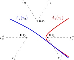
Figure 4: The hyperbola branches intersect tangentially on the degeneracy locus. This configuration can lead to poor localization accuracy when TDOAs are affected by measurement errors.

4 The $3$–dimensional Minkowski space

As discussed in Section 3, TDOA–based localization is mathematically equivalent to computing the intersection points of some hyperbola branches. This can be treated as an algebraic problem in the $x$–plane by simply considering the full hyperbolas. In this case, however, it is not easy to manipulate the system of two quadratic equations and remain in full control of all the intersection points. In particular, there could appear extra (both real and complex) intersection points with no meaning for the problem, and there is no systematic way to select the ones that are actually related to the localization.

In order to overcome such difficulties, we manipulate the equations that define the level sets $A_{i}(\tau_{i})$ (see Def. 3.3), to obtain an equivalent, partially linear, problem in a 3D space (see [12] for an introduction on the topic). In order to find the points in $A_{1}(\tau_{1})\cap A_{2}(\tau_{2})$, we need to solve the system

$$\left\{\begin{array}[]{l}\tau_{1}=d_{1}(\mathbf{x})-d_{0}(\mathbf{x}),\\ \tau_{2}=d_{2}(\mathbf{x})-d_{0}(\mathbf{x}).\end{array}\right.$$

We introduce a third auxiliary variable $\tau$, and rewrite it as

$$\left\{\begin{array}[]{l}\tau_{1}-\tau=d_{1}(\mathbf{x}),\\ \tau_{2}-\tau=d_{2}(\mathbf{x}),\\ \tau=-d_{0}(\mathbf{x}).\end{array}\right.$$

Again, this is not an algebraic problem, because of the presence of Euclidean distances. However, by squaring both sides of the equations, we obtain the polynomial system

$$\left\{\begin{array}[]{l}(\tau_{1}-\tau)^{2}=d_{1}(\mathbf{x})^{2},\\ (\tau_{2}-\tau)^{2}=d_{2}(\mathbf{x})^{2},\\ \tau^{2}=d_{0}(\mathbf{x})^{2}.\end{array}\right.$$

In geometric terms, this corresponds to studying the intersection of three cones in the 3D space described by the triplets $(x,y,\tau)$. As described in [20, 12] this problem representation is given in the space–range reference frame. For the given TDOA measurements $(\tau_{1},\tau_{2})$, a solution $(\bar{x},\bar{y},\bar{\tau})$ of the system gives an admissible position $(\bar{x},\bar{y})$ of the source in the $x$–plane and the corresponding time of emission $\bar{\tau}$ of the signal, with respect to the time of arrival at the reference microphone $\mathbf{m_{0}}$. We are actually only interested in the solutions with $\bar{\tau}\leq\rm{min}(\tau_{1},\tau_{2},0)$, i.e. in the points that lie on the three negative half–cones. Then, we can use the third equation to simplify the others, to obtain

$$\left\{\begin{array}[]{l}\mathbf{d_{10}}\cdot\mathbf{d_{0}}(\mathbf{x})-\tau_{1}\,\tau=\frac{d_{10}^{2}-\tau_{1}^{2}}{2},\\ \mathbf{d_{20}}\cdot\mathbf{d_{0}}(\mathbf{x})-\tau_{2}\,\tau=\frac{d_{20}^{2}-\tau_{2}^{2}}{2},\\[2.84526pt] d_{0}(\mathbf{x})^{2}-\tau^{2}=0,\\[2.84526pt] \tau\leq\rm{min}(\tau_{1},\tau_{2},0).\end{array}\right.$$ (12)

We conclude that, from a mathematical standpoint, that of TDOA-based localization is a semi–algebraic and partially linear problem, given by the intersection of two planes (a line) and a half–cone. This is shown in Fig. 5. Notice that the equations in system (12) involve expressions that are very similar to the standard 3D scalar products and norms, up to a minus sign in each monomial involving the variable $\tau$ or $(\tau_{1},\tau_{2})$. This suggests that, in order to describe and handle all the previous geometrical objects, an appropriate mathematical framework is the 3D Minkowski space. In the rest of the manuscript, we will explore this approach and, in particular, we will carry out our analysis using the exterior algebra formalism (see also [18, 19] for a similar analysis). We refer to Appendix A for a concise illustration of the mathematical tools we are going to use.

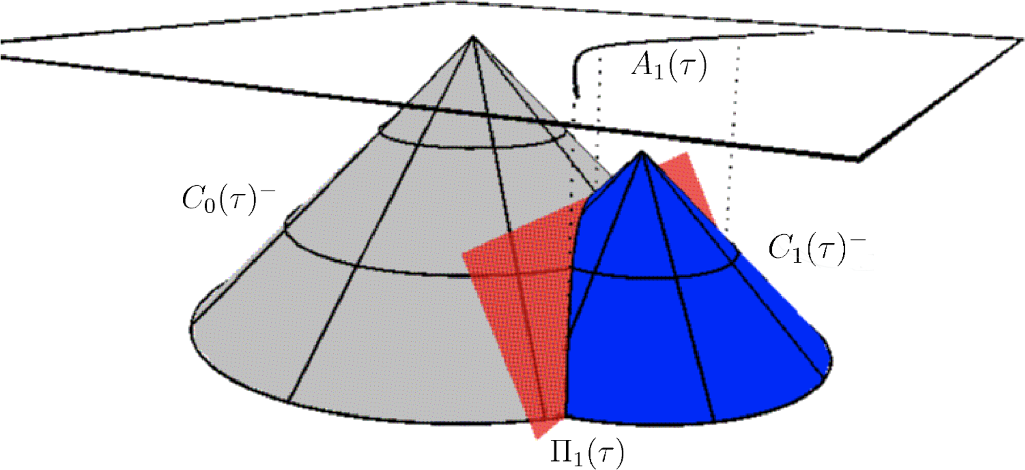
Figure 5: The intersection of the two negative half–cones $C_{0}(\boldsymbol{\tau})^{-}$ and $C_{1}(\boldsymbol{\tau})^{-}$ is a curve contained in the plane $\Pi_{1}(\boldsymbol{\tau}).$ The curve projects onto the hyperbola branch $A_{1}(\boldsymbol{\tau})$ in the $x$–plane.

Let $\mathbf{e_{1}}$, $\mathbf{e_{2}}$ and $\mathbf{e_{3}}$ be the unit vectors of the axes $x$, $y$ and $\tau$, respectively. Given the pair $\boldsymbol{\tau}=(\tau_{1},\tau_{2})$ on the $\tau$–plane, we define the points $\mathbf{M_{i}}(\boldsymbol{\tau})=(x_{i},y_{i},\tau_{i}),\ i=1,2,$ and $\mathbf{M_{0}}=(x_{0},y_{0},0)$. Given a generic point $\mathbf{X}=(x,y,\tau)$ in 3D space, the displacement vectors are defined as $\mathbf{D_{i}}(\mathbf{X},\boldsymbol{\tau})=\mathbf{X}-\mathbf{M_{i}}(\boldsymbol{\tau})$. Furthermore, we set $\mathbf{D_{ji}}(\boldsymbol{\tau})=\mathbf{M_{j}}(\boldsymbol{\tau})-\mathbf{M_{i}}(\boldsymbol{\tau})$, for $0\leq i<j\leq 2$. Notice that, in order to render the notation more uniform, we left all points and vectors as functions of $\boldsymbol{\tau}$, although many of them actually depend on a single TDOA.

Definition 4.1

For $i=0,1,2,$ we set

1. $C_{i}(\boldsymbol{\tau})=\{\mathbf{X}\in\mathbb{R}^{2,1}\ |\ \parallel\mathbf{D_{i}}(\mathbf{X},\boldsymbol{\tau})\parallel^{2}=0\};$

2. $C_{i}(\boldsymbol{\tau})^{-}=\{\mathbf{X}\in C_{i}(\boldsymbol{\tau})\ |\ \langle\mathbf{D_{i}}(\mathbf{X},\boldsymbol{\tau}),\mathbf{e_{3}}\rangle\geq 0\}.$

Moreover, for $i=1,2,$ we set

$$\Pi_{i}(\boldsymbol{\tau})=\{\mathbf{X}\in\mathbb{R}^{2,1}\ |\ \langle\mathbf{D_{i0}}(\boldsymbol{\tau}),\mathbf{D_{0}}(\mathbf{X},\boldsymbol{\tau})\rangle=\frac{1}{2}\parallel\mathbf{D_{i0}}(\boldsymbol{\tau})\parallel^{2}\}$$

and $L_{21}(\boldsymbol{\tau})=\Pi_{1}(\boldsymbol{\tau})\cap\Pi_{2}(\boldsymbol{\tau}).$

$C_{i}(\boldsymbol{\tau})$ is a right circular cone with $\mathbf{M_{i}}(\boldsymbol{\tau})$ as vertex, and $C_{i}(\boldsymbol{\tau})^{-}$ is a half–cone, while $\Pi_{i}(\boldsymbol{\tau})$ is a plane through $(\mathbf{M_{0}}(\boldsymbol{\tau})+\mathbf{M_{i}}(\boldsymbol{\tau}))/2$. Using the exterior algebra formalism (see eq. (25) and the preceding discussion in Appendix A), $\Pi_{i}$ is given by

$$\mathbf{i}_{\mathbf{D_{0}}(\mathbf{X})}(\mathbf{D_{i0}}(\boldsymbol{\tau})^{\flat})=\frac{1}{2}\parallel\mathbf{D_{i0}}(\boldsymbol{\tau})\parallel^{2}.$$ (13)

Finally, if $\mathbf{D_{10}}(\boldsymbol{\tau})$ and $\mathbf{D_{20}}(\boldsymbol{\tau})$ are linearly independent, then $L_{21}(\boldsymbol{\tau})$ is the line of equation

$$\mathbf{i}_{\mathbf{D_{0}}(\mathbf{X})}(\mathbf{D_{10}}(\boldsymbol{\tau})^{\flat}\wedge\mathbf{D_{20}}(\boldsymbol{\tau})^{\flat})=\frac{1}{2}\parallel\mathbf{D_{10}}(\boldsymbol{\tau})\parallel^{2}\mathbf{D_{20}}(\boldsymbol{\tau})^{\flat}-\frac{1}{2}\parallel\mathbf{D_{20}}(\boldsymbol{\tau})\parallel^{2}\mathbf{D_{10}}(\boldsymbol{\tau})^{\flat}.$$ (14)

We are now ready to discuss the link that exists between the geometry of the Minkowski space and the TDOA–based localization. As above, we set $A_{i}(\boldsymbol{\tau})=A_{i}(\tau_{i})$.

Theorem 4.2

Let $\pi:\mathbb{R}^{2,1}\to\mathbb{R}^{2}$ be the projection onto the $x$–plane. Then

1. $\pi(C_{0}^{-}\cap C_{i}(\boldsymbol{\tau})^{-})=A_{i}(\boldsymbol{\tau})$ if $0\leq|\tau_{i}|\leq d_{i0},$ for $i=1,2;$

2. $\pi(C_{0}^{-}\cap\Pi_{i}(\boldsymbol{\tau}))=\left\{\begin{array}[]{ll}A_{i}(\boldsymbol{\tau})&\mbox{if }-d_{i0}<\tau_{i}\leq d_{i0}\\ A_{i}(\boldsymbol{\tau})\cup r_{j}^{0}&\mbox{if }\tau_{i}=-d_{i0}\end{array}\right.$ with $i\not=j.$

Proof. Let $\mathbf{x}=\pi(\mathbf{X})$. We therefore have $\mathbf{X}=(\mathbf{x},\tau)$. According to Definition 4.1, we obtain $\mathbf{X}\in C_{0}^{-}$ if, and only if, $\parallel\mathbf{D_{0}}(\mathbf{X},\boldsymbol{\tau})\parallel^{2}=0$ and $\langle\mathbf{D_{0}}(\mathbf{X},\boldsymbol{\tau}),\mathbf{e_{3}}\rangle>0$, which means that $d_{0}(\mathbf{x})^{2}-\tau^{2}=0,\ -\tau>0$, therefore we finally obtain $d_{0}(\mathbf{x})=-\tau,\ \tau<0$. Similarly, $\mathbf{X}\in C_{i}(\boldsymbol{\tau})^{-}$ is equivalent to $d_{i}(\mathbf{x})=-(\tau-\tau_{i}),\ \tau<\tau_{i}$. As a consequence, $\mathbf{X}\in C_{0}^{-}\cap C_{i}(\boldsymbol{\tau})^{-}$ if, and only if, $d_{i}(\mathbf{x})-d_{0}(\mathbf{x})=\tau_{i},\ \tau<\min(0,\tau_{i})$, i.e. $\mathbf{x}\in A_{i}(\boldsymbol{\tau})$, therefore the first claim follows.

Then, we remark that $\mathbf{D_{i}}(\mathbf{X},\boldsymbol{\tau})=\mathbf{D_{0}}(\mathbf{X},\boldsymbol{\tau})+\mathbf{D_{i0}}(\boldsymbol{\tau})$, that implies

$$\parallel\mathbf{D_{i}}(\mathbf{X},\boldsymbol{\tau})\parallel^{2}=\parallel\mathbf{D_{0}}(\mathbf{X},\boldsymbol{\tau})\parallel^{2}+2\langle\mathbf{D_{0}}(\mathbf{X},\boldsymbol{\tau}),\mathbf{D_{i0}}(\boldsymbol{\tau})\rangle+\parallel\mathbf{D_{i0}}(\boldsymbol{\tau})\parallel^{2}.$$

Hence, $\mathbf{X}\in C_{0}\cap\Pi(\boldsymbol{\tau})$ if, and only if, $\mathbf{X}\in C_{0}\cap C_{i}(\boldsymbol{\tau}),$ and, using the first claim, we get $\pi(C_{0}^{-}\cap\Pi_{i}(\boldsymbol{\tau}))\supseteq A_{i}(\boldsymbol{\tau})$. $C_{0}^{-}\cap\Pi_{i}(\boldsymbol{\tau})$ is degenerate, precisely a half–line, if, and only if, $\mathbf{M_{0}}\in\Pi_{i}(\boldsymbol{\tau}),$ i.e. $0=\langle\mathbf{D_{i0}}(\boldsymbol{\tau}),\mathbf{0}\rangle=\frac{1}{2}\parallel\mathbf{D_{i0}}(\boldsymbol{\tau})\parallel^{2}.$ The last condition is equivalent to $\mathbf{M_{i}}(\boldsymbol{\tau})\in C_{0},$ or $\tau_{i}^{2}=d_{i0}.$ Hence, if $\tau_{i}^{2}\not=d_{i0}^{2},$ $\pi(C_{0}^{-}\cap\Pi_{i}(\boldsymbol{\tau}))$ is a hyperbola branch and the first equality follows. Otherwise, if $\tau_{i}^{2}=d_{i0}^{2},$ then $\pi(C_{0}\cap\Pi(\boldsymbol{\tau}))=r_{j}.$ It is easy to check that $(\mathbf{m_{i}},-d_{i0})\in C_{0}^{-}$ and that $(\mathbf{m_{i}},d_{i0})\in C_{0}\setminus C_{0}^{-}.$ So, $\pi(C_{0}\cap\Pi(\boldsymbol{\tau}))=A_{i}(\boldsymbol{\tau})\cup r_{j}^{0}$ if $\tau_{i}=-d_{i0}.$ $\square$

5 First properties of the image of $\boldsymbol{\tau_{2}}$

We now study the set of admissible pseudoranges, i.e. the image $\rm{Im}(\boldsymbol{\tau_{2}})$ of the TDOA map, in the $\tau$–plane. In particular, in this Section we begin with focusing on the dimension of the image and then we prove that $\mbox{Im}(\boldsymbol{\tau_{2}})$ is contained within a bounded convex set in the $\tau$–plane. These preliminary results are quite similar for both cases of generic and collinear microphone configurations, which is the reason why we collect them together in this Section. For the definition and properties of convex polytopes, see [39] among the many available references.

Theorem 5.1

$\mbox{Im}(\boldsymbol{\tau_{2}})$ is locally the $\tau$–plane.

Proof. Let us assume that $\mathbf{\bar{x}}$ is a point where $\boldsymbol{\tau_{2}}$ is regular, i.e. where the Jacobian matrix $J(\mathbf{\bar{x}})$ has rank $2$ (see Theorem 3.2). The map $\boldsymbol{\tau_{2}}$ can be written as

$$\left\{\begin{array}[]{l}d_{1}(\mathbf{x})-d_{0}(\mathbf{x})=\tau_{1}\\ d_{2}(\mathbf{x})-d_{0}(\mathbf{x})=\tau_{2}\end{array}\right.$$

and $\boldsymbol{\bar{\tau}}=\boldsymbol{\tau_{2}}(\mathbf{\bar{x}})$ is a solution of the system. The Implicit Function Theorem guarantees that there exist functions $x=x(\boldsymbol{\tau})$ and $y=y(\boldsymbol{\tau})$, which are defined in a neighborhood of $\boldsymbol{\bar{\tau}}$ and take on values in a neighborhood of $\mathbf{\bar{x}}$ so that the given system will be equivalent to

$$\left\{\begin{array}[]{l}x=x(\boldsymbol{\tau})\\ y=y(\boldsymbol{\tau})\end{array}\right.\;,$$

therefore the claim follows. $\square$

In Lemma 3.4 we showed that the TDOAs are constrained by the triangular inequalities. In the rest of this Section we will show that, as a consequence of these inequalities, $\boldsymbol{\tau_{2}}$ maps the $x$–plane onto a specific bounded region in the $\tau$–plane.

Definition 5.2

Let

$$P_{2}=\{\boldsymbol{\tau}\in\mathbb{R}^{2}|\,\|\mathbf{D_{ji}}(\boldsymbol{\tau})\|^{2}\geq 0,\ 0\leq i<j\leq 2\},$$

and $k\in\{0,1,2\}$ be different from $i,j$, for $0\leq i<j\leq 2$. We define

$$F_{k}^{+}=\{\boldsymbol{\tau}\in P_{2}|\,\|\mathbf{D_{ji}}(\boldsymbol{\tau})\|^{2}=0,\ \langle\mathbf{D_{ji}}(\boldsymbol{\tau}),\mathbf{e_{3}}\rangle<0\},$$

$$F_{k}^{-}=\{\boldsymbol{\tau}\in P_{2}|\,\|\mathbf{D_{ji}}(\boldsymbol{\tau})\|^{2}=0,\ \langle\mathbf{D_{ji}}(\boldsymbol{\tau}),\mathbf{e_{3}}\rangle>0\},$$

$$R^{0}=F_{1}^{+}\cap F_{2}^{+},\qquad R^{1}=F_{0}^{+}\cap F_{2}^{-},\qquad R^{2}=F_{0}^{-}\cap F_{1}^{-}.$$

Before we proceed with studying the relation between $P_{2}$ and $\mbox{Im}(\boldsymbol{\tau_{2}})$, let us describe the geometric properties of this set. In Fig. 6, we show some examples of $P_{2}$ (in gray), for different positions of the points $\mathbf{m_{0}}$, $\mathbf{m_{1}}$ and $\mathbf{m_{2}}$.

Theorem 5.3

$P_{2}$ is a polygon (a $2$–dimensional convex polytope). Moreover, if the points $\mathbf{m_{0}}$, $\mathbf{m_{1}}$ and $\mathbf{m_{2}}$ are not collinear, then $P_{2}$ has exactly $6$ facets $F_{k}^{\pm}$, which drop to $4$ if the points are collinear.

Proof. As a first step we notice that

$$\|\mathbf{D_{ji}}(\boldsymbol{\tau})\|^{2}=d_{ji}^{2}-(\tau_{j}-\tau_{i})^{2},$$

therefore

$$\qquad\|\mathbf{D_{ji}}(\boldsymbol{\tau})\|^{2}\geq 0\quad\Leftrightarrow\quad d_{ji}\geq|\tau_{j}-\tau_{i}|.$$ (15)

The set $P_{2}$ is a $2$–dimensional convex polytope because, according to (15), it is the intersection of half–planes and it contains an open neighborhood of $\mathbf{0}=(0,0)\in\mathbb{R}^{2}$. In fact, the coordinates of $\mathbf{0}$ satisfy all the finitely many strict inequalities defining $P_{2}$, which implies that also a sufficiently small open disc centered at $\mathbf{0}$ belongs to $P_{2}$.

In order to prove the rest of the statement, we need to show that the inequalities defining $P_{2}$ are redundant if, and only if, $\mathbf{m_{0}},\mathbf{m_{1}},\mathbf{m_{2}}$ are collinear. Let us consider

$$\left\{\begin{array}[]{l}-d_{10}\leq\tau_{1}\leq d_{10}\\ -d_{20}\leq\tau_{2}\leq d_{20}\\ -d_{21}\leq\tau_{2}-\tau_{1}\leq d_{21}\end{array}\right.\;.$$

The first two inequalities define a rectangle whose sides are parallel to the $\tau_{i}$ axes. The lines $\tau_{2}-\tau_{1}=d_{21}$ and $\tau_{2}=d_{20}$ meet at $(d_{20}-d_{21},d_{20})$, which lies between $(-d_{10},d_{20})$ and $(d_{10},d_{20})$ if, and only if, $|d_{20}-d_{21}|<d_{10}$, i.e. when the points $\mathbf{m_{0}},\mathbf{m_{1}},\mathbf{m_{2}}$ are not collinear. Through a similar reasoning we can show that, if the three points $\mathbf{m_{i}}$ are not collinear, the line $\tau_{2}-\tau_{1}=d_{21}$ meets $\tau_{1}=-d_{10}$ at $(-d_{10},d_{21}-d_{10})$, while $\tau_{2}-\tau_{1}=-d_{21}$ meets $\tau_{1}=d_{10}$ at $(d_{10},-d_{21}+d_{10})$ and $\tau_{2}=-d_{20}$ at $(d_{21}-d_{20},-d_{20})$. An easy check proves that $P_{2}$ is a hexagon of vertices $(d_{10},d_{20}),(d_{20}-d_{21},d_{20}),(-d_{10},d_{21}-d_{10}),(-d_{10},-d_{20}),(d_{21}-d_{20},-d_{20}),(d_{10},-d_{21}+d_{10})$.

On the other hand, if $\mathbf{m_{0}},\mathbf{m_{1}},\mathbf{m_{2}}$ are collinear, $P_{2}$ ends up having $4$ sides. There are three possible configurations: $(i)$ $\mathbf{m_{0}}$ lies between $\mathbf{m_{1}}$ and $\mathbf{m_{2}};$ $(ii)$ $\mathbf{m_{1}}$ lies between $\mathbf{m_{0}}$ and $\mathbf{m_{2}}$; $(iii)$ $\mathbf{m_{2}}$ lies between $\mathbf{m_{0}}$ and $\mathbf{m_{1}}$. In case $(i)$ we have that $d_{21}=d_{10}+d_{20}$, therefore $-d_{21}\leq\tau_{2}-\tau_{1}\leq d_{21}$ are redundant. In case $(ii)$ we have that $d_{20}=d_{10}+d_{21}$ and $-d_{20}\leq\tau_{2}\leq d_{20}$ give no restrictions to the others. In case $(iii)$, $-d_{10}\leq\tau_{1}\leq d_{10}$ are redundant as it follows from $d_{10}=d_{20}+d_{21}$. $\square$

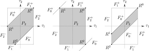
Figure 6: Left-hand side: polygon $P_{2}$ (in shaded gray) under the assumption that the points $\mathbf{m_{0}}$, $\mathbf{m_{1}}$ and $\mathbf{m_{2}}$ are not collinear. Center: polygon $P_{2}$ (in shaded gray) in the case of three collinear points with $\mathbf{m_{0}}$ between $\mathbf{m_{1}}$ and $\mathbf{m_{2}}$. Right-hand side: polygon $P_{2}$ (in shaded gray) when the sensors lie on a line, but with $\mathbf{m_{1}}$ between $\mathbf{m_{0}}$ and $\mathbf{m_{2}}$. The case with $\mathbf{m_{2}}$ between $\mathbf{m_{0}}$ and $\mathbf{m_{1}}$ can be obtained from the image on the right by swapping the role of $\tau_{1}$ and $\tau_{2}$.

For further reference, we name the vertices of the rectangle $-d_{10}\leq\tau_{1}\leq d_{10},-d_{20}\leq\tau_{2}\leq d_{20}$, recalling that $R^{0}=(d_{10},d_{20})$ (see Definition 5.2).

Definition 5.4

Let $R^{*}=(-d_{10},d_{20})$, $R^{0}_{1}=(-d_{10},-d_{20})$, and $R^{*}_{1}=(d_{10},-d_{20})$.

We are now ready to present the main result of this section.

Proposition 5.5

$\mbox{Im}(\boldsymbol{\tau_{2}})\subsetneq P_{2}$. Moreover, $\boldsymbol{\tau_{2}}^{-1}(F_{k}^{\pm})=r_{k}^{\pm}$, $k=0,1,2$, and, if $\mathbf{m_{0}},\mathbf{m_{1}},\mathbf{m_{2}}$ are not collinear, then $\boldsymbol{\tau_{2}}^{-1}(R^{k})=\mathbf{m_{k}}$, $k=0,1,2$.

Proof. The first statement is a direct consequence of Definition 5.2, relation (15) and Lemma 3.4. Let us now consider $\mathbf{x}$ such that $\pm d_{ji}=\tau_{j}(\mathbf{x})-\tau_{i}(\mathbf{x})=d_{j}(\mathbf{x})-d_{i}(\mathbf{x})$. Using Lemma 3.4 we get $\mathbf{x}\in r_{k}^{\pm}$, as claimed. As the preimage of the intersection of two sets is equal to the intersection of the respective preimages, the last statement follows from Definition 3.1. Finally, the vertices of $P_{2}$ that are different from $R^{0}$, $R^{1}$ and $R^{2}$ are not in $\mbox{Im}(\boldsymbol{\tau_{2}})$, because the corresponding half–lines do not meet, as it is easy to verify in all the possible cases. For example, if $\mathbf{m_{0}}$, $\mathbf{m_{1}}$ and $\mathbf{m_{2}}$ are not collinear, then $r_{1}^{+}$ and $r_{0}^{+}$ do not meet, which implies $(d_{20}-d_{21},d_{20})\in P_{2}\setminus\mbox{Im}(\boldsymbol{\tau_{2}})$. $\square$

6 The localization problem in the general case

In this Section we offer further insight on the TDOA map under the assumption that $\mathbf{m_{0}},\mathbf{m_{1}},\mathbf{m_{2}}$ are not collinear. Subsections 6.1 and 6.2 contain some preliminary mathematical results. In Subsection 6.1 we show how the preimages of the $\boldsymbol{\tau_{2}}$ map are strictly related to the non–positive real roots of a degree-$2$ equation, whose coefficients are polynomials in $\boldsymbol{\tau}$ (see eq. (18) and the proof of Theorem 6.16). In order to use the Descartes’ rule of signs for the characterization of the roots, in Subsection 6.2 we give the necessary background on the zero sets of such coefficients and on the sign that the polynomials take on in the $\tau$–plane. The main results of this Section are offered in Subsections 6.3 and 6.4. In the former we completely describe Im$(\boldsymbol{\tau_{2}})$ and the cardinality of each fiber, while in the latter we derive a visual representation of the different preimage regions of $\boldsymbol{\tau_{2}}$ in the $x$–plane, and find the locus where $\boldsymbol{\tau_{2}}$ is $1$–to–$1$. The two Subsections 6.3 and 6.4 also offer an interpretation of such results from the perspective of the localization problem.

This Section is, in fact, quite central for the manuscript, and the results included here are mainly proven using techniques coming from algebraic geometry. A brief presentation of the tools of algebraic geometry that are needed for this purpose is included in Appendix B. In order to improve the readability of this Section, we collected some of the proofs in Subsection 6.5.

6.1 The quadratic equation

As discussed in the previous Sections, $\boldsymbol{\tau}\in\mbox{Im}(\boldsymbol{\tau_{2}})$ if, and only if, $A_{1}(\boldsymbol{\tau})\cap A_{2}(\boldsymbol{\tau})\not=\emptyset$. According to Theorem 4.2, we have $A_{1}(\boldsymbol{\tau})\cap A_{2}(\boldsymbol{\tau})\subseteq\pi(C_{0}^{-}\cap L_{21}(\boldsymbol{\tau}))$, therefore the analysis of the intersection $C_{0}^{-}\cap L_{21}(\boldsymbol{\tau})$ plays a crucial role in characterizing the TDOA map. We begin with studying the line $L_{21}(\boldsymbol{\tau})$ of defining eq. (14).

Assuming that the microphones are not aligned, we have

$$\eqalign{\mathbf{D_{1}}(\mathbf{X},\boldsymbol{\tau})\wedge\mathbf{D_{2}}(\mathbf{X},\boldsymbol{\tau})=(\mathbf{d_{1}}(\mathbf{x})+\tau_{1}\mathbf{e_{3}})\wedge(\mathbf{d_{2}}(\mathbf{x})+\tau_{2}\mathbf{e_{3}})=\cr=\mathbf{d_{1}}(\mathbf{x})\wedge\mathbf{d_{2}}(\mathbf{x})+(\tau_{2}\mathbf{d_{1}}(\mathbf{x})-\tau_{1}\mathbf{d_{2}}(\mathbf{x}))\wedge\mathbf{e_{3}}\neq 0}$$ (16)

because $\mathbf{d_{1}}(\mathbf{x})$ and $\mathbf{d_{2}}(\mathbf{x})$ are linearly independent. Consequently $\mathbf{D_{1}}(\mathbf{X},\boldsymbol{\tau})$ and $\mathbf{D_{2}}(\mathbf{X},\boldsymbol{\tau})$ are linearly independent as well for every $\boldsymbol{\tau}\in\mathbb{R}^{2}$. Let

$$\boldsymbol{\Omega}=\mathbf{D_{10}}(\boldsymbol{\tau})\wedge\mathbf{D_{20}}(\boldsymbol{\tau})\wedge\mathbf{e_{3}}=\mathbf{d_{10}}\wedge\mathbf{d_{20}}\wedge\mathbf{e_{3}}\neq 0\;,$$ (17)

which is a 3–form (see Section A.2 in Appendix A). With no loss of generality, we can assume that $\boldsymbol{\Omega}$ is positively oriented, i.e. $\boldsymbol{\Omega}=k\boldsymbol{\omega}$ with $k>0$, therefore $\langle\boldsymbol{\Omega},\boldsymbol{\omega}\rangle=-k<0$.

Lemma 6.1

For any $\boldsymbol{\tau}\in\mathbb{R}^{2}$, $L_{21}(\boldsymbol{\tau})=\Pi_{1}(\boldsymbol{\tau})\cap\Pi_{2}(\boldsymbol{\tau})$ is a line. A parametric representation of $L_{21}(\boldsymbol{\tau})$ is $\mathbf{X}(\lambda;\boldsymbol{\tau})=\mathbf{L_{0}}(\boldsymbol{\tau})+\lambda\mathbf{v}(\boldsymbol{\tau})$, where

$$\qquad\mathbf{v}(\boldsymbol{\tau})=\ast(\mathbf{D_{10}}(\boldsymbol{\tau})\wedge\mathbf{D_{20}}(\boldsymbol{\tau}))=\ast((\mathbf{d_{10}}\wedge\mathbf{d_{20}})+(\tau_{2}\mathbf{d_{10}}-\tau_{1}\mathbf{d_{20}})\wedge\mathbf{e_{3}})$$

and the displacement vector of $\mathbf{L_{0}}(\boldsymbol{\tau})$ is

$$\qquad\mathbf{D_{0}}(\mathbf{L_{0}}(\boldsymbol{\tau})) = \frac{1}{2\ast\boldsymbol{\Omega}}\ast\!\left(\left(\|\mathbf{D_{10}}(\boldsymbol{\tau})\|^{2}\mathbf{D_{20}}(\boldsymbol{\tau})-\|\mathbf{D_{20}}(\boldsymbol{\tau})\|^{2}\mathbf{D_{10}}(\boldsymbol{\tau})\right)\wedge\mathbf{e_{3}}\right)=$$

$$= -\frac{\ast\left(\left(\|\mathbf{D_{10}}(\boldsymbol{\tau})\|^{2}\mathbf{d_{20}}-\|\mathbf{D_{20}}(\boldsymbol{\tau})\|^{2}\mathbf{d_{10}}\right)\wedge\mathbf{e_{3}}\right)}{2\|\mathbf{d_{10}}\wedge\mathbf{d_{20}}\|}.$$

Proof. See Subsection 6.5. $\square$

Remark 6.2

The point $\mathbf{L_{0}}(\boldsymbol{\tau})$ is the intersection between $L_{21}(\boldsymbol{\tau})$ and the $x$–plane. In fact, from the properties of the Hodge $\ast$ operator, we know that the component of $\mathbf{D_{0}}(\mathbf{L_{0}}(\boldsymbol{\tau}))$ along $\mathbf{e_{3}}$ is zero.

We can turn our attention to the study of $C_{0}^{-}\cap L_{21}(\boldsymbol{\tau})$. From the definition of $C_{0}$ and Lemma 6.1 follows that a point $\mathbf{X}(\lambda;\boldsymbol{\tau})$ of the line $L_{21}(\boldsymbol{\tau})$ lies on $C_{0}$ if the vector $\mathbf{D_{0}}(\mathbf{L_{0}}(\boldsymbol{\tau}))+\lambda\mathbf{v}(\boldsymbol{\tau})$ is isotropic with respect to the bilinear form $b$. This means that $\|\mathbf{D_{0}}(\mathbf{L_{0}}(\boldsymbol{\tau}))+\lambda\mathbf{v}(\boldsymbol{\tau})\|^{2}=0$ or, more explicitly,

$$\|\mathbf{v}(\boldsymbol{\tau})\|^{2}\lambda^{2}+2\lambda\langle\mathbf{D_{0}}(\mathbf{L_{0}}(\boldsymbol{\tau})),\mathbf{v}(\boldsymbol{\tau})\rangle+\|\mathbf{D_{0}}(\mathbf{L_{0}}(\boldsymbol{\tau}))\|^{2}=0.$$ (18)

This equation in $\lambda\in\mathbb{R}$ has a degree that does not exceed $2$, and coefficients that depend on $\boldsymbol{\tau}$.

Definition 6.3

Let

1. $a(\boldsymbol{\tau})=\|\mathbf{v}(\boldsymbol{\tau})\|^{2}=\|\tau_{2}\mathbf{d_{10}}-\tau_{1}\mathbf{d_{20}}\|^{2}-\|\mathbf{d_{10}}\wedge\mathbf{d_{20}}\|^{2};$

2. $b(\boldsymbol{\tau})=\langle\mathbf{D_{0}}(\mathbf{L_{0}}(\boldsymbol{\tau})),\mathbf{v}(\boldsymbol{\tau})\rangle=\displaystyle\frac{\langle\tau_{2}\mathbf{d_{10}}-\tau_{1}\mathbf{d_{20}},\|\mathbf{D_{20}}(\boldsymbol{\tau})\|^{2}\mathbf{d_{10}}-\|\mathbf{D_{10}}(\boldsymbol{\tau})\|^{2}\mathbf{d_{20}}\rangle}{2\|\mathbf{d_{10}}\wedge\mathbf{d_{20}}\|};$

3. $c(\boldsymbol{\tau})=\|\mathbf{D_{0}}(\mathbf{L_{0}}(\boldsymbol{\tau}))\|^{2}=\displaystyle\frac{\left\|\|\mathbf{D_{10}}(\boldsymbol{\tau})\|^{2}\mathbf{d_{20}}-\|\mathbf{D_{20}}(\boldsymbol{\tau})\|^{2}\mathbf{d_{10}}\right\|^{2}}{4\|\mathbf{d_{10}}\wedge\mathbf{d_{20}}\|^{2}}.$

Eq. (18) can be rewritten as

$$a(\boldsymbol{\tau})\lambda^{2}+2b(\boldsymbol{\tau})\lambda+c(\boldsymbol{\tau})=0.$$ (19)

The explicit solution of eq. (18) will be derived in Subsection 6.4.

6.2 The study of the coefficients

In order to study the solutions of the quadratic equation (18), we need to use Descartes’ rule of signs. To apply it, we first describe the zero set of the coefficients $a(\boldsymbol{\tau})$, $b(\boldsymbol{\tau})$, and $c(\boldsymbol{\tau})$; then we study the sign of these coefficients wherever they do not vanish. As stated above, the main mathematical tools that are used in this Subsection come from algebraic geometry because $a(\boldsymbol{\tau})$, $b(\boldsymbol{\tau})$ and $c(\boldsymbol{\tau})$ are polynomials with real coefficients (see Appendix B for a short introduction or [13, 22, 29]).

Let us first describe the vanishing locus of $c(\boldsymbol{\tau})$, over both $\mathbb{R}$, where it is particularly simple, and $\mathbb{C}$.

Proposition 6.4

$c(\boldsymbol{\tau})\geq 0$ for every $\boldsymbol{\tau}\in\mathbb{R}^{2}$. Moreover, $c(\boldsymbol{\tau})=0$ if and only if $\boldsymbol{\tau}\in\{R^{0},R^{*},R^{*}_{1},R^{0}_{1}\}$. On the complex field $\mathbb{C}$, $c(\boldsymbol{\tau})$ factors as the product of two degree-$2$ polynomials.

Proof. See Subsection 6.5. $\square$

In order to analyze the sign of $a(\boldsymbol{\tau})$, we need to introduce some notation.

Definition 6.5

We define three subsets of the $\tau$–plane, according to the sign of $a(\boldsymbol{\tau})$:

• $E=\{\boldsymbol{\tau}\in\mathbb{R}^{2}\ |\ a(\boldsymbol{\tau})=0\};$

• $E^{+}=\{\boldsymbol{\tau}\in\mathbb{R}^{2}\ |\ a(\boldsymbol{\tau})>0\};$

• $E^{-}=\{\boldsymbol{\tau}\in\mathbb{R}^{2}\ |\ a(\boldsymbol{\tau})<0\}$.

Proposition 6.6

$E\subset P_{2}$ is an ellipse centered in $\mathbf{0}=(0,0)$, and it represents the only conic that is tangent to all sides of the hexagon $P_{2}$.

Proof. See Subsection 6.5. $\square$

The ellipse $E$ and some specific points on the polytope $P_{2}$ are shown in Fig. 7. As the tangency points will eventually show up in the study of the vanishing locus of $b(\boldsymbol{\tau})$, we define them here for further reference.

Definition 6.7

Let $0\leq i,j,k\leq 2$ with $k<j$ and $k\neq j$. Then

$$T_{i}^{+}=\left(\langle\mathbf{d_{10}},\mathbf{\tilde{d_{jk}}}\rangle,\langle\mathbf{d_{20}},\mathbf{\tilde{d_{jk}}}\rangle\right)\quad\mbox{ and }\quad T_{i}^{-}=\left(-\langle\mathbf{d_{10}},\mathbf{\tilde{d_{jk}}}\rangle,-\langle\mathbf{d_{20}},\mathbf{\tilde{d_{jk}}}\rangle\right),$$

where, according to our current notation, $\mathbf{\tilde{d_{jk}}}=\frac{\mathbf{d_{jk}}}{d_{jk}}$.

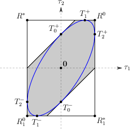
Figure 7: The ellipse $E$ (in blue) is tangent to each side of the hexagon $P_{2}$ (in gray). We have $11$ distinguished points: the center $\mathbf{0}$ of $E$, the six tangency points $T_{i}^{\pm},i=0,1,2$, and the vertices of the rectangle $R_{1}^{0},R^{0},R^{*}$ and $R_{1}^{*}$.

Remark 6.8

For every non-collinear choice of $\mathbf{m_{0}}$, $\mathbf{m_{1}}$, $\mathbf{m_{2}}$, $E$ is smooth. In fact, $\nabla a(\boldsymbol{\tau})=(0,0)$ is the homogeneous linear system

$$\left\{\begin{array}[]{l}d_{20}^{2}\tau_{1}-\langle\mathbf{d_{10}},\mathbf{d_{20}}\rangle\tau_{2}=0\\ -\langle\mathbf{d_{10}},\mathbf{d_{20}}\rangle\tau_{1}+d_{10}^{2}\tau_{2}=0\end{array}\right.$$

whose only solution is $\mathbf{0}\notin E$, because the matrix of the coefficients of the variables has determinant $\|\mathbf{d_{10}}\wedge\mathbf{d_{20}}\|^{2}\not=0$.

We conclude the analysis of the sign of $a(\boldsymbol{\tau})$ by noticing that the set $E^{-}$ contains the origin $\mathbf{0}$, therefore it is the bounded connected component of $\mathbb{R}^{2}\setminus E$. Similarly, $R^{0}\in E^{+}$ therefore $E^{+}$ is the unbounded connected component of $\mathbb{R}^{2}\setminus E$.

The analysis of the sign of the last coefficients $b(\boldsymbol{\tau})$ is a bit more involved. Let us define the notations as done for $a(\boldsymbol{\tau})$.

Definition 6.9

We define three subsets of the $\tau$–plane, according to the sign of $b(\boldsymbol{\tau})$:

• $C=\{\boldsymbol{\tau}\in\mathbb{R}^{2}\ |\ b(\boldsymbol{\tau})=0\};$

• $C^{+}=\{\boldsymbol{\tau}\in\mathbb{R}^{2}\ |\ b(\boldsymbol{\tau})>0\};$

• $C^{-}=\{\boldsymbol{\tau}\in\mathbb{R}^{2}\ |\ b(\boldsymbol{\tau})<0\}$.

As our aim is to study the relative position of $P_{2}$ and the sets $C$, $C^{+}$, and $C^{-}$, we need more of an in-depth understanding of the curve $C$ (see Figure 8 for some examples of this curve). We will first analyze the role of the $11$ distinguished points marked in Fig. 7 for the study of $c(\boldsymbol{\tau})=0$ and $a(\boldsymbol{\tau})=0$ in connection with $b(\boldsymbol{\tau})=0$. We will then look for special displacement positions of $\mathbf{m_{0}}$, $\mathbf{m_{1}}$ and $\mathbf{m_{2}}$, which force $C$ to be non–irreducible. In fact, the irreducibility of $C$ has an impact on the topological properties of $C^{+}$ and $C^{-}$, particularly on their connectedness by arcs. We will finally study the connected components of $C$.

Proposition 6.10

$C$ is a cubic curve with $2$–fold rotational symmetry with respect to $\mathbf{0}$, which contains $T_{0}^{\pm}$, $T_{1}^{\pm}$, $T_{2}^{\pm}$, $R^{0}$, $R^{0}_{1}$, $R^{*}$, $R^{*}_{1}$ and $\mathbf{0}$. The tangent lines to $C$ at $R^{0}$, $R^{0}_{1}$, $R^{*}$, $R^{*}_{1}$ are orthogonal to $F_{0}^{+}$, therefore $C$ is smooth at the above four points. Finally, $C$ transversally intersects both $E$ and the lines that support the sides of $P_{2}$.

Proof. See Subsection 6.5. $\square$

Proposition 6.11

$C$ is a smooth curve, unless $d_{10}=d_{20}$. In this case $C$ is the union of the line $L:\tau_{1}+\tau_{2}=0$ and the conic $E^{\prime}:\tau_{1}^{2}-(\langle\mathbf{\tilde{d}_{10}},\mathbf{\tilde{d}_{20}}\rangle+1)\tau_{1}\tau_{2}+\tau_{2}^{2}+d_{10}^{2}(\langle\mathbf{\tilde{d}_{10}},\mathbf{\tilde{d}_{20}}\rangle-1)=0$.

Proof. See Subsection 6.5. $\square$

For the sake of completeness, we now investigate the uniqueness of this cubic curve by showing that $C$ is completely determined by the positions of the points $\mathbf{m_{0}}$, $\mathbf{m_{1}}$, $\mathbf{m_{2}}$.

Proposition 6.12

$C$ is the unique cubic curve that contains the points $T_{0}^{\pm}$, $T_{1}^{\pm}$, $T_{2}^{\pm}$, $\mathbf{0}$, $R^{0}$, $R^{0}_{1}$, $R^{*}$, $R^{*}_{1}$.

Proof. See Subsection 6.5. $\square$

Remark 6.13

Due to the $2$–fold rotational symmetry around $\mathbf{0}$, and the fact that $C$ is smooth at $\mathbf{0}$, we can conclude that $\mathbf{0}$ is an inflectional point for $C$.

The cubic curve $C$, where smooth, has genus $1$. Therefore, in the $\tau$–plane, it can have either $1$ or $2$ ovals, in compliance with Harnack’s Theorem B.31 (see Fig. 8). Depending on the position of $\mathbf{m_{0}}$, $\mathbf{m_{1}}$, $\mathbf{m_{2}}$, both cases are possible. Following standard notation, the two ovals are called $C_{o}$, the odd oval, and $C_{e}$, the even one (this could be missing), and, at least in the projective plane $\mathbb{P}_{\mathbb{R}}^{2}$, they are the connected components of $C$. The importance of studying the connected components of $C$ rests on the fact that $C$ divides every neighborhood of a point $P\in C$ in two sets, one in $C^{+}$, the other in $C^{-}$. Therefore, we need to locate $C_{o}$ and $C_{e}$ with respect to $P_{2}.$

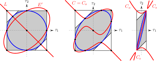
Figure 8: Examples of cubics $C$: on the left-hand side it is singular. In the centre it is an oval and on the right-hand side are two ovals. The curve $E$ is shown in blue, $C$ in red, and the hexagon $P_{2}$ in shaded gray. The $11$ distinguished points are marked in the first two pictures, but not in the last one because $4$ of them are very close to each other on the upper–right vertex of the rectangle, and similarly for the $4$ ones, which are close to the opposite vertex. In all the three cases $P_{2}$ is an hexagon, but it exhibits two very short sides in the right-hand picture.

Proposition 6.14

The points $T_{0}^{\pm},T_{1}^{\pm},T_{2}^{\pm},\mathbf{0},R^{0},R^{*},R^{0}_{1},R^{*}_{1}$ belong to the same connected component $C_{o}$ of $C$, which is the only one that intersects $P_{2}$.

Proof. See Subsection 6.5. $\square$

Now we can complete the study of the sign of $b(\boldsymbol{\tau})$ within $P_{2}$. Let us first assume that $C$ is smooth. Due to the rotational symmetry of $C$, the component $C_{o}$ is connected in the affine plane $\mathbb{R}^{2}$ as well, and it divides the $\tau$–plane in two disjoint sets, which we name $C_{o}^{+}$ and $C_{o}^{-}$. Due to Proposition 6.14, $b(\boldsymbol{\tau})$ does not change sign on $P_{2}\cap C_{o}^{+}$ and $P_{2}\cap C_{o}^{-}$, therefore we have $P_{2}\cap C^{+}=P_{2}\cap C_{o}^{+}$ and $P_{2}\cap C^{-}=P_{2}\cap C_{o}^{-}$ (possibly with $C_{o}^{+},C_{o}^{-}$ in swapped order). In particular, evaluating $b(\boldsymbol{\tau})$ at the vertices of $P_{2}$, we have that $C_{o}^{+}$ is the connected component of $\mathbb{R}^{2}\setminus C_{o}$ containing $R^{1},R^{2}$.

Finally, if $C$ is singular we have $C=L\cup E^{\prime}$ (see Fig. 8). There are four disjoint regions in the $\tau$–plane having different signs. Again by evaluating $b(\boldsymbol{\tau})$ at the vertices of $P_{2}$, we obtain that $C^{+}$ is the union of the region outside $E^{\prime}$ in the half plane containing $R^{1},R^{2}$ plus the region inside $E^{\prime}$ in the complementary half plane.

6.3 The image of $\boldsymbol{\tau_{2}}$

In this Subsection we achieve one of the main goals of the manuscript, as we derive the complete and explicit description of Im$(\boldsymbol{\tau_{2}})$, i.e. the set of admissible TDOAs. These results are summarized in Fig. 9. In the following, we will denote the closure of a set $U$ as $\bar{U}$ and its interior as $\mathring{U}$.

Definition 6.15

The set $\mathring{P_{2}}\cap E^{+}\cap C^{+}$ is the union of $three$ disjoint connected components that we name $U_{0},U_{1},U_{2},$ where $R^{i}\in\bar{U}_{i}$ for $i=0,1,2$.

Theorem 6.16

$\mbox{Im}(\boldsymbol{\tau_{2}})=E^{-}\cup\bar{U}_{0}\cup\bar{U}_{1}\cup\bar{U}_{2}\setminus\{T_{0}^{\pm},T_{1}^{\pm},T_{2}^{\pm}\}.$ Moreover,

$$|\boldsymbol{\tau_{2}}^{-1}(\boldsymbol{\tau})|=\cases{2&if $\boldsymbol{\tau}\in U_{0}\cup U_{1}\cup U_{2}$,\\ 1&if $\boldsymbol{\tau}\in\mbox{Im}(\boldsymbol{\tau_{2}})\setminus U_{0}\cup U_{1}\cup U_{2}$.}$$

Proof. Consider the equation (19)

$$a(\boldsymbol{\tau})\lambda^{2}+2b(\boldsymbol{\tau})\lambda+c(\boldsymbol{\tau})=0,$$

with $\boldsymbol{\tau}\in P_{2}$. The reduced discriminant $\Delta(\boldsymbol{\tau})/4=b(\boldsymbol{\tau})^{2}-a(\boldsymbol{\tau})c(\boldsymbol{\tau})$ is a degree-$6$ polynomial that vanishes if $L_{21}(\boldsymbol{\tau})$ is tangent to the cone $C_{0}$. According to Theorem 4.2, this condition is equivalent to $A_{1}(\boldsymbol{\tau})$ and $A_{2}(\boldsymbol{\tau})$ intersecting tangentially. According to Proposition 3.6, this happens exactly if $\mathbf{x}\in r_{0}^{\pm}\cup r_{1}^{\pm}\cup r_{2}^{\pm}$. Hence, $\boldsymbol{\tau}\in\boldsymbol{\tau_{2}}(r_{0}^{\pm}\cup r_{1}^{\pm}\cup r_{2}^{\pm})=F_{0}^{\pm}\cup F_{1}^{\pm}\cup F_{2}^{\pm}$, which implies $\Delta(\boldsymbol{\tau})=0$ if, and only if, $\boldsymbol{\tau}\in\partial P_{2}$. On the other hand, $\Delta(\mathbf{0})=-a(\mathbf{0})c(\mathbf{0})>0$ because $\mathbf{0}\in E^{-}$, therefore $\Delta(\boldsymbol{\tau})>0$ for $\boldsymbol{\tau}\in\mathring{P}_{2}$. As a consequence, equation (19) has real solutions for any $\boldsymbol{\tau}\in P_{2}$.

According to Theorem 4.2, we are looking for $\boldsymbol{\tau}$ that satisfies $C_{0}^{-}\cap L_{21}(\boldsymbol{\tau})\not=\emptyset$:

$$\qquad\qquad\eqalign{0\leq\langle\mathbf{D_{0}}(\mathbf{L_{0}}(\boldsymbol{\tau}))+\lambda\mathbf{v}(\boldsymbol{\tau}),\mathbf{e_{3}}\rangle=\langle\mathbf{D_{0}}(\mathbf{L_{0}}(\boldsymbol{\tau})),\mathbf{e_{3}}\rangle+\lambda\langle\mathbf{v}(\boldsymbol{\tau}),\mathbf{e_{3}}\rangle=\cr\quad=\lambda\langle*(\mathbf{d_{10}}\wedge\mathbf{d_{20}}),\mathbf{e_{3}}\rangle=\lambda\langle\ast(\mathbf{d_{10}}\wedge\mathbf{d_{20}}),\ast(\mathbf{e_{1}}\wedge\mathbf{e_{2}})\rangle=\cr\quad=-\lambda\langle\mathbf{d_{10}}\wedge\mathbf{d_{20}},\mathbf{e_{1}}\wedge\mathbf{e_{2}}\rangle=\lambda\langle\mathbf{d_{10}}\wedge\mathbf{d_{20}}\wedge\mathbf{e_{3}},\boldsymbol{\omega}\rangle=\lambda\langle\boldsymbol{\Omega},\boldsymbol{\omega}\rangle,}$$

which narrows down to $\lambda\leq 0$, as $\langle\boldsymbol{\Omega},\boldsymbol{\omega}\rangle<0$.

Let us first consider the case $\lambda=0$, which is equivalent to $c(\boldsymbol{\tau})=0$. From Proposition 6.4, we know that $c(\boldsymbol{\tau})\geq 0$ for any $\boldsymbol{\tau}\in P_{2},$ and $c(\boldsymbol{\tau})=0$ if, and only if, $\boldsymbol{\tau}\in\{R^{0},R^{*},R^{0}_{1},R^{*}_{1}\}$. At the four considered points, also $b(\boldsymbol{\tau})=0$ and $\Delta(\boldsymbol{\tau})=0.$ Hence, $\lambda=0$ is the only solution with multiplicity $2,$ if $\boldsymbol{\tau}=R^{0}$ or $\boldsymbol{\tau}=R^{0}_{1},$ the other two points not being in $P_{2}.$ However, the half–lines $r_{1}^{+}$ and $r_{2}^{+}$ meet at $\mathbf{x}=\mathbf{m_{0}},$ while $r_{1}^{-}\cap r_{2}^{-}=\emptyset$. Consequently, $\boldsymbol{\tau_{2}}^{-1}(R^{0})=\mathbf{m_{0}}$, while $R^{0}_{1}\notin\mbox{Im}(\boldsymbol{\tau_{2}})$.

Let us now assume $\lambda\not=0,$ i.e. $c(\boldsymbol{\tau})>0$, and consider all the possible cases, one at a time. The main (and essentially unique) tool is Descartes’ rule of signs for determining the number of positive roots of a polynomial equation, with real coefficients and real roots.

Case (i):

$a(\boldsymbol{\tau})=b(\boldsymbol{\tau})=0$.
Eq. (19) has no solution, therefore $E\cap C=\{T_{0}^{\pm},T_{1}^{\pm},T_{2}^{\pm}\}$ is not in $\mbox{Im}(\boldsymbol{\tau_{2}})$.

Case (ii):

$a(\boldsymbol{\tau})=0,b(\boldsymbol{\tau})\not=0$.
Eq. (19) has the only solution $\lambda=-c(\boldsymbol{\tau})/2b(\boldsymbol{\tau})$ for each $\boldsymbol{\tau}\in E\setminus\{T_{0}^{\pm},T_{1}^{\pm},T_{2}^{\pm}\}.$ Moreover, $\lambda<0$ if, and only if, $b(\boldsymbol{\tau})>0$ i.e. $\boldsymbol{\tau}\in E\cap C^{+}=(\partial U_{0}\cup\partial U_{1}\cup\partial U_{2})\cap E\setminus\{T_{0}^{\pm},T_{1}^{\pm},T_{2}^{\pm}\}.$

Case (iii):

$a(\boldsymbol{\tau})<0$.
Equation (19) has one negative root and one positive root, thus $E^{-}\subset\mbox{Im}(\boldsymbol{\tau_{2}})$ and $|\boldsymbol{\tau_{2}}^{-1}(\boldsymbol{\tau})|=1$ for each $\boldsymbol{\tau}\in E^{-}.$

Case (iv):

$a(\boldsymbol{\tau})>0,b(\boldsymbol{\tau})<0$.
Eq. (19) has two positive roots, thus $E^{+}\cap C^{-}\cap\mbox{Im}(\boldsymbol{\tau_{2}})=\emptyset.$

Case (v):

$a(\boldsymbol{\tau})>0,b(\boldsymbol{\tau})>0,\Delta(\boldsymbol{\tau})=0$.
Eq. (19) has one negative root with multiplicity $2,$ thus $|\boldsymbol{\tau_{2}}^{-1}(\boldsymbol{\tau})|=1$ for each $\boldsymbol{\tau}\in E^{+}\cap C^{+}\cap\partial P_{2}.$ In particular, $\boldsymbol{\tau_{2}}^{-1}(R^{j})=\mathbf{m_{j}}$ for $j=1,2.$

Case (vi):

$a(\boldsymbol{\tau})>0,b(\boldsymbol{\tau})>0,\Delta(\boldsymbol{\tau})>0$.
Eq. (19) has two distinct negative roots, therefore $|\boldsymbol{\tau_{2}}^{-1}(\boldsymbol{\tau})|=2$ for any $\boldsymbol{\tau}\in U_{0}\cup U_{1}\cup U_{2}$. $\square$

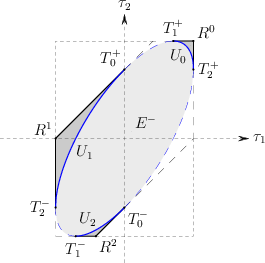
Figure 9: The image of $\boldsymbol{\tau_{2}}$ is the gray subset of $P_{2}$. In the light gray region marked as $E^{-}$ the map $\boldsymbol{\tau_{2}}$ is $1$–to–$1$, while in the medium gray regions $U_{0}\cup U_{1}\cup U_{2}$ the map $\boldsymbol{\tau_{2}}$ is $1$–to–$2$. The continuous part of $\partial P_{2}$ and $E$, and the vertices $R^{i}$, are in the image, where $\boldsymbol{\tau_{2}}$ is $1$–to–$1$. The dashed part of $\partial P_{2}$ and $E$, and the tangency points $T_{i}^{\pm}$, do not belong to Im($\boldsymbol{\tau_{2}}$). We remark that the triangles $U_{0},U_{1},U_{2}$ stay on the same connected component of $\mathbb{R}^{2}\setminus C_{o}$ (see Fig. 8)

Remark 6.17

Theorem 6.16 agrees with Theorem 4.2. The exact relationship between $A_{1}(\boldsymbol{\tau})\cap A_{2}(\boldsymbol{\tau})$ and $\pi(C_{0}^{-}\cap L_{21}(\boldsymbol{\tau}))$ is the following:

(1)

If $\boldsymbol{\tau}\notin F_{2}^{-}\cup F_{1}^{-}$, then $\pi(C_{0}^{-}\cap L_{21}(\boldsymbol{\tau}))=A_{1}(\boldsymbol{\tau})\cap A_{2}(\boldsymbol{\tau})$.

(2)

If $\boldsymbol{\tau}\in F_{2}^{-}\setminus\{R_{1}^{0}\},$ then $\tau_{1}=-d_{10}$ and $-d_{20}<\tau_{2}\leq d_{21}-d_{10}$. Thus

$$\pi(C_{0}^{-}\cap L_{21}(\boldsymbol{\tau}))=(A_{1}(\boldsymbol{\tau})\cap A_{2}(\boldsymbol{\tau}))\cup(r_{2}^{0}\cap A_{2}(\boldsymbol{\tau})),$$

where $A_{1}(\boldsymbol{\tau})=r_{2}^{-}$. If $\mathbf{x}\in r_{2}^{0}\cap A_{2}(\boldsymbol{\tau})$, then $d_{0}(\mathbf{x})=d_{10}-d_{1}(\mathbf{x})$ and

$$\tau_{2}(\mathbf{x})=d_{2}(\mathbf{x})-d_{0}(\mathbf{x})=d_{2}(\mathbf{x})+d_{1}(\mathbf{x})-d_{10}\geq d_{21}-d_{10},$$

where we used the triangular inequality. It follows that $\tau_{2}(\mathbf{x})=d_{21}-d_{10}$ and $\mathbf{x}=\mathbf{m_{1}}$, so $r_{2}^{0}\cap A_{2}(\boldsymbol{\tau})=A_{1}(\boldsymbol{\tau})\cap A_{2}(\boldsymbol{\tau})$ and, again, $\pi(C_{0}^{-}\cap L_{21}(\boldsymbol{\tau}))=A_{1}(\boldsymbol{\tau})\cap A_{2}(\boldsymbol{\tau})$. The case $\boldsymbol{\tau}\in F_{1}^{-}\setminus\{R_{1}^{0}\}$ is similar.

(3)

If $\boldsymbol{\tau}=R_{1}^{0}\notin\mbox{Im}(\boldsymbol{\tau_{2}}),$ then $A_{1}(\boldsymbol{\tau})\cap A_{2}(\boldsymbol{\tau})=\emptyset$ while $\pi(C_{0}^{-}\cap L_{21}(\boldsymbol{\tau}))=r_{1}^{0}\cup r_{2}^{0}=\mathbf{m_{0}}.$

Theorem 6.16 can be nicely interpreted in terms of the two-dimensional and the three-dimensional intersection problems. Here we use some standard Minkowski and relativistic conventions used, for example, in [3, 43].

1. $\boldsymbol{\tau}\in E$ if, and only if, $\mathbf{v}(\boldsymbol{\tau})$ is isotropic, or light–like. In this case, the line $L_{21}(\boldsymbol{\tau})$ is parallel to a generatrix of the cone, therefore it meets $C_{0}$ at an ideal point. On the $x$–plane this means that the level sets $A_{1}(\boldsymbol{\tau})$ and $A_{2}(\boldsymbol{\tau})$ have one parallel asymptote. With respect to the localization problem, $\boldsymbol{\tau}\in E$ means that there could exist a source whose distance from the microphones is large compared to $d_{10}$ and $d_{20}$. Along $E$, the two TDOAs are not independent and we are able to recover information only about the direction of arrival of the signal, and not on the source location. Things complicate further if $\boldsymbol{\tau}\in E\cap\mbox{Im}(\boldsymbol{\tau_{2}})$, as the level sets $A_{1}(\boldsymbol{\tau})$ and $A_{2}(\boldsymbol{\tau})$ also meet at a point at finite distance, corresponding to another admissible source location.

2. $\boldsymbol{\tau}\in E^{-}$ if, and only if $\mathbf{v}(\boldsymbol{\tau})$ is time–like, pointing to the interior of the cone $C_{0}$. In this case, the line $L_{21}(\boldsymbol{\tau})$ intersects both half–cones and, on the $x$–plane, the level sets $A_{1}(\boldsymbol{\tau})$ and $A_{2}(\boldsymbol{\tau})$ meet at a single point. This is the most desirable case for localization purposes: a $\boldsymbol{\tau}$ corresponds to a unique source position $\mathbf{x}$.

3. $\boldsymbol{\tau}\in E^{+}$ if, and only if, $\mathbf{v}(\boldsymbol{\tau})$ is space–like, pointing to the exterior of the cone $C_{0}$. In this case, the line $L_{21}(\boldsymbol{\tau})$ intersects only one half–cone, depending on the position of the point $\mathbf{L_{0}}(\boldsymbol{\tau})$ and the direction of $\mathbf{v}(\boldsymbol{\tau})$. On the $x$–plane, the level sets $A_{1}(\boldsymbol{\tau}),A_{2}(\boldsymbol{\tau})$ either do not intersect or intersect at two distinct points. In the last case, for a given $\boldsymbol{\tau}$ there are two admissible source positions. Following the discussion at point (i), a source runs away to infinity as $\boldsymbol{\tau}$ gets close to $E$, while the other remains at a finite position, which suggests a possible way to distinguish between them if one has some a-priori knowledge on the source location. Finally, we observe that the two solutions overlap if $\boldsymbol{\tau}\in\partial P_{2}$, which corresponds to $\mathbf{x}$ in the degeneracy locus.

If $\boldsymbol{\tau}\in E^{-}$, the localization is still possible even in a noisy scenario, but we experience a loss in precision and stability as $\boldsymbol{\tau}$ approach $E$ (see also the discussion in Section 9).

6.4 The inverse image

We are now ready to reverse the analysis. In fact, the description of Im($\boldsymbol{\tau_{2}}$) allows us to analyze the dual situation in the physical $x$–plane. For any given $\boldsymbol{\tau}\in\mbox{Im}(\boldsymbol{\tau_{2}})$ and a negative solution $\lambda$ of eq. (18), we have the corresponding preimage in the $x$–plane

$$\mathbf{x}(\boldsymbol{\tau})=\mathbf{L_{0}}(\boldsymbol{\tau})+\lambda\ast((\tau_{2}\mathbf{d_{10}}-\tau_{1}\mathbf{d_{20}})\wedge\mathbf{e_{3}}),$$ (20)

where $\ast((\tau_{2}\mathbf{d_{10}}-\tau_{1}\mathbf{d_{20}})\wedge\mathbf{e_{3}})$ is the projection of $\mathbf{v}(\boldsymbol{\tau})$ on the subspace spanned by $\mathbf{e_{1}},\mathbf{e_{2}}$. Roughly speaking, we can identify two distinct regions: the preimage of the interior of the ellipse, where the TDOA map is $1$–to–$1$ and the source localization is possible, and the preimage of the three triangles $U_{i},\ i=0,1,2$, where the map is $2$–to–$1$ and there is no way to locate the source. The region of transition is also known in the literature as the bifurcation region [19]. In this subsection we offer a complete geometric description of the above sets.

Notice that that formula (20) gives the exact solutions $\mathbf{x}$ to the localization problem for any given measurements $\boldsymbol{\tau}$, and it can be used as the starting point and building block for a local error propagation analysis in the case of noisy measurements or even with sensor calibration uncertainty.

Definition 6.18

Let $E$ be the ellipse in the $\tau$–plane defined by $a(\boldsymbol{\tau})=0$. We call $\tilde{E}$ its inverse image contained in the $x$–plane, and we refer to it as the bifurcation curve.

As we said in the discussion at the end of Subsection 6.3, for $\boldsymbol{\tau}\in E$ we have an admissible source position at an ideal point of the $x$–plane and, possibly, one more at a finite distance from the sensors. In the affine plane, the curve $\tilde{E}$ is exactly the set of these last points. According to Definition 6.18, $\tilde{E}$ is the preimage of $E$, therefore it can be studied using formula (20). We recall that for $\boldsymbol{\tau}\in E$ we have $a(\boldsymbol{\tau})=0$, therefore eq. (18) has a unique solution in $\lambda(\boldsymbol{\tau})=-c(\boldsymbol{\tau})/2b(\boldsymbol{\tau})$, which corresponds to the unique preimage

$$\mathbf{x}(\boldsymbol{\tau})=\mathbf{L_{0}}(\boldsymbol{\tau})-\frac{c(\boldsymbol{\tau})}{2b(\boldsymbol{\tau})}\ast((\tau_{2}\mathbf{d_{10}}-\tau_{1}\mathbf{d_{20}})\wedge\mathbf{e_{3}}).$$ (21)

In the next Theorem, we show that the function (21) restricted on $E$ is a rational parametrization of degree $5$ of the bifurcation curve $\tilde{E}$. This means that $\tilde{E}$ admits a characterization as an algebraic curve.

Theorem 6.19

$\tilde{E}$ is a rational degree–$5$ curve, whose ideal points are the ones of the lines $r_{0},r_{1},r_{2}$ and the cyclic points of $\mathbb{P}_{\mathbb{C}}^{2}.$

Proof. See Subsection 6.5. $\square$

In Fig. 10 we show two examples of the quintic $\tilde{E}$. The real part of $\tilde{E}$ consists of three disjoint arcs, one for each arc of $E$ contained in $\mbox{Im}(\boldsymbol{\tau_{2}})$. The points $\mathbf{m_{0}},\mathbf{m_{1}},\mathbf{m_{2}}$ do not belong to $\tilde{E}$, as their images via $\boldsymbol{\tau_{2}}$ are not on $E$. Notice that no arc is bounded, as $\tilde{E}$ has genus $0$. In particular, when $\boldsymbol{\tau}$ approaches a point $T_{i}^{\pm}$ in $E\cap C$ the denominator of $\mathbf{x}(\boldsymbol{\tau})$ approaches to zero and $\tilde{E}$ goes to infinity. As for the smoothness of $\tilde{E}$, the curve has no self–intersection because each point of the $x$–plane has one image in the $\tau$–plane. Furthermore, it is quite easy to show that cusps are not allowed on $\tilde{E}$ either. In fact, $E$ is regularly parameterized and the Jacobian matrix of $\boldsymbol{\tau_{2}}$ is invertible on $\tilde{E}$, which implies the regularity of $\mathbf{x}(\boldsymbol{\tau})$. Quite clearly, on the complex plane $\tilde{E}$ is bound to have singular points, as $\tilde{E}$ is an algebraic rational quintic curve. In Appendix C we include the source code in Singular [23] language for computing the Cartesian equation (further analysis of the properties of the bifurcation curve is contained in [21]).

From Fig. 9 and Fig. 10, we immediately recognize what was assessed through simulations and for a specific sensor configuration in [51]. These results, however, have been here derived in closed form and for arbitrary sensor geometries, which allows us to characterise the pre–image in an exhaustive fashion.

The curve $\tilde{E}$ separates the regions of the $x$–plane where the map $\boldsymbol{\tau_{2}}$ is $1$–to–$1$ or $2$–to–$1$. We complete the analysis in terms of TDOA–based localization after introducing and analyzing the preimage of the open subsets $E^{-},U_{0},U_{1},U_{2}$ of Im$(\boldsymbol{\tau_{2}})$.

Definition 6.20

Let $\tilde{U}_{i}$ be the inverse image of $U_{i}$ via $\boldsymbol{\tau_{2}}$, for $i=0,1,2$, and $\tilde{E}^{-}$ be the inverse image of $E^{-}$.

The continuity of $\boldsymbol{\tau_{2}}$ implies that $\tilde{E}^{-}$, $\tilde{U}_{0}$, $\tilde{U}_{1}$, $\tilde{U}_{2}$ are open subsets of the $x$–plane, which are separated by the three arcs of $\tilde{E}$. Let $F(x,y)=0$ be a Cartesian equation of $\tilde{E}$: a point $\mathbf{x}\in\tilde{E}^{-}$ if $F(\mathbf{x})F(\mathbf{m_{0}})<0$, while $\mathbf{x}\in\tilde{U}_{0}\cup\tilde{U}_{1}\cup\tilde{U}_{2}$ if $F(\mathbf{x})F(\mathbf{m_{0}})>0$. Now, let us focus on the open sets $\tilde{U}_{i}$. In this case, without loss of generality, we consider $i=0$, the other two ones having the same properties.

Proposition 6.21

$\tilde{U}_{0}$ has two connected components separated by $r_{1}^{+}\cup r_{2}^{+}$, and $\boldsymbol{\tau_{2}}$ is $1$–to–$1$ on each of them.

Proof. See Subsection 6.5. $\square$

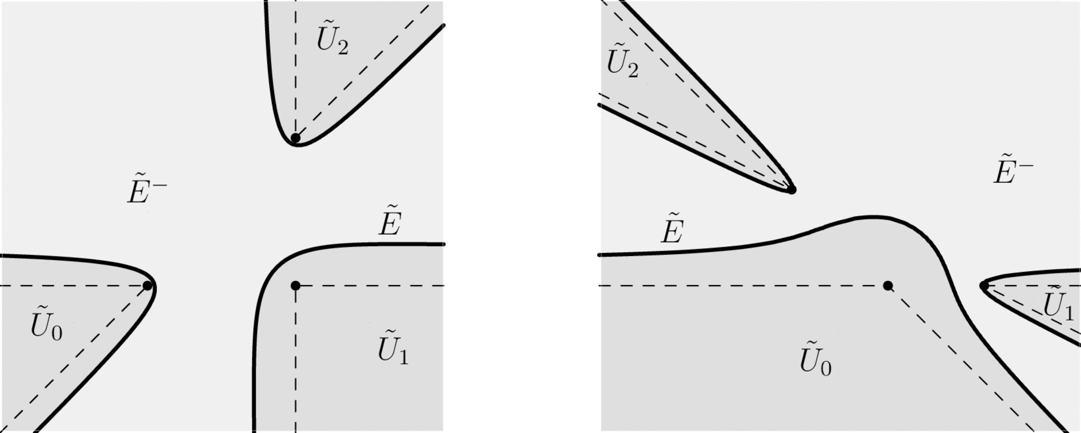
Figure 10: Two examples of the different localization regions and the quintic $\tilde{E}$ in the $x$–plane. The microphones $\mathbf{m_{0}},\mathbf{m_{1}}$ and $\mathbf{m_{2}}$ are the in the points marked with black dots. Locations of the microphones are $\mathbf{m_{0}}=(0,0),\ \mathbf{m_{1}}=(2,0)$, $\mathbf{m_{2}}=(2,2)$ and $\mathbf{m_{2}}=(-2,2)$ on the left and the right, respectively. Each quintic $\tilde{E}$ separates the light gray region $\tilde{E}^{-}$, where the map $\boldsymbol{\tau_{2}}$ is 1–1 and it is possible to localize the source, and the dark gray region $\tilde{U}_{0}\cup\tilde{U}_{1}\cup\tilde{U}_{2}$, where $\boldsymbol{\tau_{2}}$ is 2–1 and the localization is not unique. The dashed lines represent the degeneracy locus of $\boldsymbol{\tau_{2}}$.

Remark 6.22

The previous Proposition can be restated by saying that $\boldsymbol{\tau_{2}}:\tilde{U_{i}}\to U_{i}$ is a double cover, for every $i=0,1,2$. The ramification locus is the union of the two half–lines through $\mathbf{m_{i}},$ while the branching locus is union of the two facets of $P_{2}$ through $R^{i}$.

The source localization is possible if $\boldsymbol{\tau}\in E^{-}$ and, consequently, $\mathbf{x}\in\tilde{E}^{-}$. Otherwise, assume $\boldsymbol{\tau}\in U_{0}$. According to Proposition 6.21, there are two admissible sources in the two disjoint components of $\tilde{U}_{0}$. As $\boldsymbol{\tau}$ comes close to $E$, one of its inverse images approaches a point on $\tilde{E}$, while the other one goes to infinity. Conversely, if $\boldsymbol{\tau}$ approaches $\partial P_{2}$, the inverse images of $\boldsymbol{\tau}$ come closer to each other and converge to a point on the degeneracy locus $r_{1}^{+}\cup r_{2}^{+}$. As we said above, in a realistic noisy scenario, we end up with poor localization in the proximity of $\tilde{E}$.

6.5 Proofs of the results

Proof of Lemma 6.1. As remarked before eq. (14), $L_{21}(\boldsymbol{\tau})$ is a line because $\mathbf{D_{10}}(\boldsymbol{\tau})$ and $\mathbf{D_{20}}(\boldsymbol{\tau})$ are linearly independent. Thus, the equation of $L_{21}(\boldsymbol{\tau})$ is (14):

$$\mathbf{i}_{\mathbf{D_{0}}(\mathbf{X})}(\mathbf{D_{10}}(\boldsymbol{\tau})^{\flat}\wedge\mathbf{D_{20}}(\boldsymbol{\tau})^{\flat})=\frac{1}{2}\parallel\mathbf{D_{10}}(\boldsymbol{\tau})\parallel^{2}\mathbf{D_{20}}(\boldsymbol{\tau})^{\flat}-\frac{1}{2}\parallel\mathbf{D_{20}}(\boldsymbol{\tau})\parallel^{2}\mathbf{D_{10}}(\boldsymbol{\tau})^{\flat}.$$

A vector $\mathbf{v}(\boldsymbol{\tau})$ is parallel to $L_{21}(\boldsymbol{\tau})$ if it is a solution of

$$\mathbf{i}_{\mathbf{v}(\boldsymbol{\tau})}(\mathbf{D_{10}}(\boldsymbol{\tau})^{\flat}\wedge\mathbf{D_{20}}(\boldsymbol{\tau})^{\flat})=0$$

From Corollary A.6, this is equivalent to

$$\mathbf{v}(\boldsymbol{\tau})=t\ast(\mathbf{D_{10}}(\boldsymbol{\tau})^{\flat}\wedge\mathbf{D_{20}}(\boldsymbol{\tau})^{\flat})^{\sharp}=t\ast(\mathbf{D_{10}}(\boldsymbol{\tau})\wedge\mathbf{D_{20}}(\boldsymbol{\tau}))$$

for $t\in\mathbb{R}.$ We prove the first claim of the Lemma by setting $t=1.$

Then, let $\mathbf{L_{0}}(\boldsymbol{\tau})$ be the intersection point between $L_{21}(\boldsymbol{\tau})$ and the $x$–plane. This implies that

$$\mathbf{i}_{\mathbf{D_{0}}(\mathbf{L_{0}}(\boldsymbol{\tau}))}\,\boldsymbol{\Omega}^{\flat}=\frac{1}{2}\left(\parallel\mathbf{D_{10}}(\boldsymbol{\tau})\parallel^{2}\mathbf{D_{20}}(\boldsymbol{\tau})^{\flat}-\parallel\mathbf{D_{20}}(\boldsymbol{\tau})\parallel^{2}\mathbf{D_{10}}(\boldsymbol{\tau})^{\flat}\right)\wedge\mathbf{e_{3}}^{\flat}.$$

Therefore, the second claim follows from Lemma A.7. $\square$

Proof of Proposition 6.4. As a real function, $c(\boldsymbol{\tau})\geq 0$ because $\|\mathbf{D_{10}}(\boldsymbol{\tau})\|^{2}\mathbf{d_{20}}-\|\mathbf{D_{20}}(\boldsymbol{\tau})\|^{2}\mathbf{d_{10}}$ is in the subspace spanned by $\mathbf{e_{1}},\mathbf{e_{2}},$ where $b$ is positive-defined, and $\mathbf{d_{10}}\wedge\mathbf{d_{20}}$ is parallel to $\mathbf{e_{1}}\wedge\mathbf{e_{2}}$, whose module is equal to $1$. Furthermore, $\mathbf{d_{10}},\mathbf{d_{20}}$ are linearly independent, thus $c(\boldsymbol{\tau})=0$ if, and only if, $\|\mathbf{D_{10}}(\boldsymbol{\tau})\|^{2}=\|\mathbf{D_{20}}(\boldsymbol{\tau})\|^{2}=0,$ i.e. $\tau_{1}^{2}=d_{10}^{2},\ \tau_{2}^{2}=d_{20}^{2}$, and the claim follows.

The gradient of $c(\boldsymbol{\tau})$ is

$$\nabla c(\boldsymbol{\tau})=\frac{1}{\|\mathbf{d_{10}}\wedge\mathbf{d_{20}}\|^{2}}\left(\langle-\tau_{1}\mathbf{d_{20}},\|\mathbf{D_{10}}(\boldsymbol{\tau})\|^{2}\mathbf{d_{20}}-\|\mathbf{D_{20}}(\boldsymbol{\tau})\|^{2}\mathbf{d_{10}}\rangle,\right.$$

$$\left.\langle\tau_{2}\mathbf{d_{10}},\|\mathbf{D_{10}}(\boldsymbol{\tau})\|^{2}\mathbf{d_{20}}-\|\mathbf{D_{20}}(\boldsymbol{\tau})\|^{2}\mathbf{d_{10}}\rangle\right),$$

therefore it vanishes if $\|\mathbf{D_{10}}(\boldsymbol{\tau})\|^{2}=\|\mathbf{D_{20}}(\boldsymbol{\tau})\|^{2}=0.$ Hence, in $\mathbb{A}^{2}_{\mathbb{C}},$ $c(\boldsymbol{\tau})=0$ is a quartic algebraic curve with four singular points, thus it cannot be irreducible (see Theorem B.22). After some simple computations, we obtain

$$c(\boldsymbol{\tau})=\left(d_{20}e^{-i\theta}(\tau_{1}^{2}-d_{10}^{2})-d_{10}e^{i\theta}(\tau_{2}^{2}-d_{20}^{2})\right)\left(d_{20}e^{i\theta}(\tau_{1}^{2}-d_{10}^{2})-d_{10}e^{-i\theta}(\tau_{2}^{2}-d_{20}^{2})\right)$$

where $2\theta\in(0,\pi)$ is the angle between $\mathbf{d_{10}}$ and $\mathbf{d_{20}}.$ $\square$

Proof of Proposition 6.6. The equation that defines $E$, i.e.

$$a(\boldsymbol{\tau})=-\|\mathbf{d_{10}}\wedge\mathbf{d_{20}}\|^{2}+\|\tau_{2}\mathbf{d_{10}}-\tau_{1}\mathbf{d_{20}}\|^{2}=0\;,$$

has degree $2$, therefore $E$ is a conic in the $\tau$–space. Considering the assumption of non-collinearity, $\|\tau_{2}\mathbf{d_{10}}-\tau_{1}\mathbf{d_{20}}\|^{2}$ is a positively-defined quadratic form and $\|\mathbf{d_{10}}\wedge\mathbf{d_{20}}\|^{2}>0$. $E$ is therefore a non-degenerate ellipse containing real points, whose center is at $\mathbf{0}$. Moreover, it is a simple matter of computation to verify that the intersection between $E$ and $F_{i}^{+}$ is the point $T_{i}^{+}$ with multiplicity $2$, for $i=0,1,2$, and analogously for $F_{i}^{-}$ and $T_{i}^{-}$. $E$ is therefore tangent to each side of $P_{2}$. This implies also that $E\subset P_{2}$. In order to prove the uniqueness of $E$, we embed the $\tau$–plane $\mathbb{R}^{2}$ into a projective plane $\mathbb{P}^{2}_{\mathbb{R}},$ and take the dual projective plane $\check{\mathbb{P}}^{2}_{\mathbb{R}}$ (see Definition B.24). In $\check{\mathbb{P}}^{2}_{\mathbb{R}}$ there exists one conic through the $6$ points corresponding to the sides of $P_{2}$ and it is the dual conic $\check{E}$ (see Definition B.25 and Proposition B.26). Moreover, $\check{E}$ is unique by Corollary B.29. We conclude that the uniqueness of $\check{E}$ is equivalent to the uniqueness of $E$. $\square$

Proof of Proposition 6.10. $C$ is defined by the degree–$3$ polynomial equation

$$\bar{b}(\boldsymbol{\tau})=\langle\tau_{2}\mathbf{d_{10}}-\tau_{1}\mathbf{d_{20}},\|\mathbf{D_{20}}(\boldsymbol{\tau})\|^{2}\mathbf{d_{10}}-\|\mathbf{D_{10}}(\boldsymbol{\tau})\|^{2}\mathbf{d_{20}}\rangle=0,$$

therefore it is a cubic curve. It is easy to verify that

• the equation does not change if we replace $\tau_{i}$ with $-\tau_{i},i=1,2$, therefore $C$ has a $2$–fold rotational symmetry with respect to $\mathbf{0}$;

• $C$ contains all the $11$ points of the statement.

The partial derivatives of $\bar{b}$ are

$$\frac{\partial\bar{b}}{\partial\tau_{1}}=-\langle\mathbf{d_{20}},\|\mathbf{D_{20}}(\boldsymbol{\tau})\|^{2}\mathbf{d_{10}}-\|\mathbf{D_{10}}(\boldsymbol{\tau})\|^{2}\mathbf{d_{20}}\rangle+\langle\tau_{2}\mathbf{d_{10}}-\tau_{1}\mathbf{d_{20}},2\tau_{1}\mathbf{d_{20}}\rangle,$$

$$\frac{\partial\bar{b}}{\partial\tau_{2}}=\langle\mathbf{d_{10}},\|\mathbf{D_{20}}(\boldsymbol{\tau})\|^{2}\mathbf{d_{10}}-\|\mathbf{D_{10}}(\boldsymbol{\tau})\|^{2}\mathbf{d_{20}}\rangle-\langle\tau_{2}\mathbf{d_{10}}-\tau_{1}\mathbf{d_{20}},2\tau_{2}\mathbf{d_{10}}\rangle.$$

After simple calculations, we obtain $\nabla\bar{b}(R^{0})=2d_{10}d_{20}\left(d_{10}d_{20}-\langle\mathbf{d_{10}},\mathbf{d_{20}}\rangle\right)(1,1)$ and $\nabla\bar{b}(R^{*})=-2d_{10}d_{20}\left(d_{10}d_{20}+\langle\mathbf{d_{10}},\mathbf{d_{20}}\rangle\right)(1,1).$ The gradient of $\bar{b}$ is therefore non-zero at both $R^{0}$ and $R^{*},$ i.e. $R^{0}$ and $R^{*}$ are smooth on $C.$ Moreover, the tangent lines to $C$ at $R^{0}$ and $R^{*}$ are orthogonal to $(1,1)$ therefore they are orthogonal to $F_{0}^{+}.$ For symmetry, the same holds at $R^{0}_{1}$ and $R^{*}_{1}.$

In compliance with Bézout’s Theorem B.16, $C$ and $E$ meet at $6$ points after embedding the $\tau$–plane into $\mathbb{P}^{2}_{\mathbb{C}}$, but $C\cap E=\{T_{0}^{\pm},T_{1}^{\pm},T_{2}^{\pm}\}$, thus $C$ and $E$ intersect transversally. Moreover, we use Bézout’s Theorem also to prove that $C$ is not tangent to any line among $F_{2}^{\pm},$ and $F_{1}^{\pm},$ because the points where the curve $C$ meets each line are known.

Finally, the line containing $F_{0}^{+}$ meets $C$ at $T_{0}^{+}$ plus two other points whose coordinates solve $\tau_{2}=\tau_{1}+d_{21},(d_{21}\tau_{1}-\langle\mathbf{d_{21}},\mathbf{d_{10}}\rangle)^{2}+\|\mathbf{d_{10}}\wedge\mathbf{d_{20}}\|^{2}=0,$ therefore they cannot be real. As a consequence, according to Bézout’s Theorem, we obtain that $C$ and $F_{0}^{+}$ are not tangent. By symmetry, $F_{0}^{-}$ is not tangent to $C$ either. $\square$

Proof of Proposition 6.11. The gradient at $\mathbf{0}$ is $\nabla\bar{b}(\mathbf{0})=(-d_{20}^{2}\langle\mathbf{d_{21}},\mathbf{d_{10}}\rangle,d_{10}^{2}\langle\mathbf{d_{21}},\mathbf{d_{20}}\rangle)\not=(0,0).$ Hence, if $C$ is not smooth, there are at least two singular points, because of the $2$–fold rotational symmetry, and so $C$ is reducible. As $C$ contains $T_{0}^{\pm},T_{1}^{\pm},T_{2}^{\pm},R^{0},R^{*},R^{0}_{1},R^{*}_{1},\mathbf{0},$ the only possible splitting of $C$ is $E^{\prime}\cup L,$ with $L$ the line through $R^{*},R^{*}_{1},\mathbf{0},T_{0}^{\pm},$ and $E^{\prime}$ the conic through $T_{2}^{\pm},T_{1}^{\pm},R^{0},R^{0}_{1}.$ The point $T_{0}^{+}$ is collinear with $\mathbf{0}$ and $R^{*}$ if, and only if, there exists $t\in\mathbb{R}$ such that

$$\left(\langle\mathbf{d_{10}},\mathbf{\tilde{d}_{21}}\rangle,\langle\mathbf{d_{20}},\mathbf{\tilde{d}_{21}}\rangle\right)=t(-d_{10},d_{20}),$$

therefore $t=\langle\mathbf{\tilde{d}_{20}},\mathbf{\tilde{d}_{21}}\rangle$ and $(d_{20}-d_{10})(\langle\mathbf{d_{10}},\mathbf{d_{20}}\rangle+d_{10}d_{20})=0.$ Since $\mathbf{m_{0}},\mathbf{m_{1}},\mathbf{m_{2}}$ are not collinear, the second factor is non–zero and $C$ is singular if, and only if, $d_{10}=d_{20}.$ The equations of $L$ and $E^{\prime}$ are then straightforward. $\square$

Proof of Proposition 6.12. If $C$ is not smooth, any cubic curve containing the given points contains the line $L,$ according to Bézout’s Theorem. The remaining points lie on a unique conic $E^{\prime},$ therefore $C=E^{\prime}\cup L$ is unique.

Let us now assume that $C$ is smooth. We embed the $\tau$–plane into $\mathbb{P}^{2}_{\mathbb{C}},$ and let $X=\{T_{0}^{\pm},T_{1}^{\pm},T_{2}^{\pm}\}$ and $Y=\{\mathbf{0},R^{0},R^{0}_{1},R^{*},R^{*}_{1}\}.$ The defining ideal $I_{X}$ of $X$ is generated by $a_{h}(\boldsymbol{\tau}),\bar{b}_{h}(\boldsymbol{\tau})$ obtained by homogenizing $a(\boldsymbol{\tau})$ and $\bar{b}(\boldsymbol{\tau}),$ because $X=E\cap C$, as proven earlier (see Theorem B.30). The ideal $I_{Y}$ of $Y$ is generated by a degree $2$ and two degree $3$ homogeneous polynomials (see Theorem B.30). Let $L_{1}$ be the line through $R^{0},R^{0}_{1},\mathbf{0},$ $L_{2}$ be the line through $R^{*},R^{*}_{1},$ and let $Q=L_{1}\cup L_{2}$. $Q$ is a reducible conic that is singular at $\mathbf{0}.$ With abuse of notation, we also call $Q$ the defining polynomial of $Q$ and so $Q\in I_{Y}$ by Definition B.27. Moreover, $Y\subset C,$ and so $\bar{b}_{h}\in I_{Y},$ as well. Finally, let $C^{\prime}$ be a further cubic curve, whose defining polynomial is equal to $C^{\prime},$ with abuse of notation, so that $I_{Y}=\langle Q,\bar{b}_{h},C^{\prime}\rangle.$

Claim: $C^{\prime}$ is not a combination of $Q$, $a_{h}$, and $\bar{b}_{h}.$

If we assume the contrary, we have $C^{\prime}=q_{1}a_{h}+q_{2}Q+q_{3}\bar{b}_{h}$ with $\deg(q_{1})=\deg(q_{2})=1$, and $\deg(q_{3})=0$. Consequently, we have $q_{1}(p)=0$ for every $p\in Y,$ because $a_{h}(p)\not=0$ for each $p\in Y$. So, $q_{1}\in I_{Y}$ therefore $q_{1}=0$ because $I_{Y}$ does not contain linear forms. Then, $C^{\prime}$ is a combination of $Q$ and $\bar{b}_{h},$ but this is not possible because $C^{\prime}$ is a minimal generator of $I_{Y},$ therefore the claim holds true.

Hence, $I_{X}+I_{Y}$ is minimally generated by $a_{h},Q,\bar{b}_{h},C^{\prime}.$ Moreover, since two conics meet at four points, $(\mathbb{C}[\tau_{0},\tau_{1},\tau_{2}]/(a_{h},Q))_{3}$ has dimension $4,$ and we obtain

$$\dim_{\mathbb{C}}\left(\frac{\mathbb{C}[\tau_{0},\tau_{1},\tau_{2}]}{I_{X}+I_{Y}}\right)_{3}=10-8=2.$$

From the exactness of the short sequence of vector spaces (27)

$$0\to\left(\frac{\mathbb{C}[\tau_{0},\tau_{1},\tau_{2}]}{I_{X}\cap I_{Y}}\right)_{3}\to\left(\frac{\mathbb{C}[\tau_{0},\tau_{1},\tau_{2}]}{I_{X}}\right)_{3}\oplus\left(\frac{\mathbb{C}[\tau_{0},\tau_{1},\tau_{2}]}{I_{Y}}\right)_{3}\to\left(\frac{\mathbb{C}[\tau_{0},\tau_{1},\tau_{2}]}{I_{X}+I_{Y}}\right)_{3}\to 0$$

we conclude that the dimension of the first item is $6+5-2=9$ and, finally, $\dim_{\mathbb{C}}\left(I_{X}\cap I_{Y}\right)_{3}=\dim_{\mathbb{C}}\left(\mathbb{C}[\tau_{0},\tau_{1},\tau_{2}]\right)_{3}-\dim_{\mathbb{C}}\left(\frac{\mathbb{C}[\tau_{0},\tau_{1},\tau_{2}]}{I_{X}\cap I_{Y}}\right)_{3}=10-9=1.$ $\square$

Proof of Proposition 6.14. We embed the $\tau$–plane into $\mathbb{P}^{2}_{\mathbb{R}}.$ The oval $C_{o}$ meets all the lines of the projective plane either in $1$ or in $3$ points, up to count the points with their intersection multiplicity, as discussed after Harnack’s Theorem B.31 in Appendix B. This implies that $C_{o}$ contains the inflectional point $\mathbf{0}$ of $C$. Moreover, from the proof of Proposition 6.10, the lines supporting $F_{0}^{\pm}$ meet $C$ at $1$ point each, thus $T_{0}^{\pm}\in C_{o}$.

The possible second oval $C_{e}$ meets every line at an even number of points ($0$ is allowed) and it cannot meet $C_{o}$. By contradiction, let us assume that $R^{*}\in C_{e}$. Hence, the line $F_{2}^{-}$ meets $C_{e}$ either at $T_{2}^{-}$ or $R^{0}_{1}$. This implies that $C_{e}$ meets the line $F_{0}^{+}$, which is a contradiction. We conclude that $R^{*}$ and, symmetrically, $R^{*}_{1}$ lie on $C_{o}$.

Again by contradiction, we assume that $R^{0}\in C_{e}$. By looking at the intersection points of $C_{e}$ with the sides of $P_{2}$, we obtain $T_{1}^{+},T_{2}^{+}\in C_{e}$ and, symmetrically, $R^{0}_{1},T_{1}^{-},T_{2}^{-}\in C_{e}$. We also observe that $C_{e}$ meets the tangent line to $C$ at $R^{0}$ exclusively at the point $R^{0}$ itself, and the same holds true at $R^{0}_{1}$. As $C_{e}$ does not meet $F_{0}^{\pm}$, $C_{e}$ is constrained into the quadrangle formed by $F_{0}^{\pm}$ and the tangent lines to $C$ at $R^{0},R^{0}_{1}$. This quadrangle contains $\mathbf{0}$, therefore either $C_{e}$ is the union of two disjoint ovals, or $C_{e}$ meets $C_{o}$. Both cases are not allowed, thus $R^{0}\in C_{o}$. This implies that all the remaining points lie on $C_{o}$ and the first claim is proven.

We finish the proof by noting that $C_{e}$ does not meet any side of $P_{2}$ and, on the other hand, $C_{e}$ cannot be contained in $P_{2}.$ $\square$

Proof of Theorem 6.19. If $\boldsymbol{\tau}\in E$, its preimage is given by (21):

$$\mathbf{x}(\boldsymbol{\tau})=\mathbf{L_{0}}(\boldsymbol{\tau})-\frac{c(\boldsymbol{\tau})}{2b(\boldsymbol{\tau})}\ast((\tau_{2}\mathbf{d_{10}}-\tau_{1}\mathbf{d_{20}})\wedge\mathbf{e_{3}}).$$

Hence, $\mathbf{x}(\boldsymbol{\tau})$ gives a point in the $x$–plane both if $\boldsymbol{\tau}\in E\cap\mbox{Im}(\boldsymbol{\tau_{2}})$ and if $\boldsymbol{\tau}\in E\setminus(\mbox{Im}(\boldsymbol{\tau_{2}})\cup C).$ Moreover, because of the symmetry properties of the polynomials and vectors involved, we have $\mathbf{x}(-\boldsymbol{\tau})=\mathbf{x}(\boldsymbol{\tau})$, which means that $\mathbf{x}(\boldsymbol{\tau})$ is a $2$–to–$1$ map from $E$ to $\tilde{E}.$

In order to obtain a parametrization of $\tilde{E}$, we consider a parametrization of $E$ via the pencil of lines through $\mathbf{0}.$ Let $\tau_{1}=\mu_{1}t,\tau_{2}=\mu_{2}t$ be a line through $\mathbf{0}$ in the $\tau$–plane, with $\boldsymbol{\mu}=(\mu_{1},\mu_{2})\in\mathbb{R}^{2}\setminus\{(0,0)\}.$ The line intersects the ellipse $E$ at the two points $t=\pm\|\mathbf{d_{10}}\wedge\mathbf{d_{20}}\|/\|\mu_{2}\mathbf{d_{10}}-\mu_{1}\mathbf{d_{20}}\|$, which are symmetrical with respect to $\mathbf{0}$. Let $P_{0}(\boldsymbol{\mu})=\|\mu_{2}\mathbf{d_{10}}-\mu_{1}\mathbf{d_{20}}\|^{2}$. This is a degree–$2$ homogeneous polynomial that vanishes at the ideal points of $E$, therefore it is irreducible over $\mathbb{R}$. By substituting $\boldsymbol{\tau}=\frac{\|\mathbf{d_{10}}\wedge\mathbf{d_{20}}\|}{\sqrt{P_{0}(\boldsymbol{\mu})}}\boldsymbol{\mu},$ all the functions depend on $\boldsymbol{\mu},$ therefore we obtain

$$\|\mathbf{D_{10}}(\boldsymbol{\mu})\|^{2}=\frac{1}{P_{0}(\boldsymbol{\mu})}\langle\mu_{1}\mathbf{d_{20}}-\mu_{2}\mathbf{d_{10}},\mathbf{d_{10}}\rangle^{2},$$

$$\|\mathbf{D_{20}}(\boldsymbol{\mu})\|^{2}=\frac{1}{P_{0}(\boldsymbol{\mu})}\langle\mu_{1}\mathbf{d_{20}}-\mu_{2}\mathbf{d_{10}},\mathbf{d_{20}}\rangle^{2}$$

which are both ratios of degree–$2$ homogeneous polynomials. For our convenience, we set $P_{1}(\boldsymbol{\mu})=\langle\mu_{1}\mathbf{d_{20}}-\mu_{2}\mathbf{d_{10}},\mathbf{d_{10}}\rangle^{2}$ and $P_{2}(\boldsymbol{\mu})=\langle\mu_{1}\mathbf{d_{20}}-\mu_{2}\mathbf{d_{10}},\mathbf{d_{20}}\rangle^{2}.$ As $\boldsymbol{\tau}$ depends on $\boldsymbol{\mu}$, the polynomials $b(\boldsymbol{\tau}),c(\boldsymbol{\tau})$ can be computed as depending on $\boldsymbol{\mu}$, obtaining

$$c(\boldsymbol{\mu})=\frac{1}{4\|\mathbf{d_{10}}\wedge\mathbf{d_{20}}\|^{2}P_{0}(\boldsymbol{\mu})^{2}}\|P_{1}(\boldsymbol{\mu})\mathbf{d_{20}}-P_{2}(\boldsymbol{\mu})\mathbf{d_{10}}\|^{2},$$

$$b(\boldsymbol{\mu})=\frac{1}{2\sqrt{P_{0}(\boldsymbol{\mu})^{3}}}\langle\mu_{2}\mathbf{d_{10}}-\mu_{1}\mathbf{d_{20}},P_{2}(\boldsymbol{\mu})\mathbf{d_{10}}-P_{1}(\boldsymbol{\mu})\mathbf{d_{20}}\rangle=$$

$$=\frac{1}{2\sqrt{P_{0}(\boldsymbol{\mu})^{3}}}\langle\mu_{2}\mathbf{d_{10}}-\mu_{1}\mathbf{d_{20}},\mathbf{d_{10}}\rangle\langle\mu_{2}\mathbf{d_{10}}-\mu_{1}\mathbf{d_{20}},\mathbf{d_{20}}\rangle\langle\mu_{2}\mathbf{d_{10}}-\mu_{1}\mathbf{d_{20}},\mathbf{d_{21}}\rangle.$$

Moreover,

$$\ast((\tau_{2}\mathbf{d_{10}}-\tau_{1}\mathbf{d_{20}})\wedge\mathbf{e_{3}})=\frac{\|\mathbf{d_{10}}\wedge\mathbf{d_{20}}\|}{\sqrt{P_{0}(\boldsymbol{\mu})}}\ast((\mu_{2}\mathbf{d_{10}}-\mu_{1}\mathbf{d_{20}})\wedge\mathbf{e_{3}})$$

and

$$\mathbf{D_{0}}(\mathbf{L_{0}}(\boldsymbol{\mu}))=-\frac{1}{2\|\mathbf{d_{10}}\wedge\mathbf{d_{20}}\|P_{0}(\boldsymbol{\mu})}\ast\left((P_{1}(\boldsymbol{\mu})\mathbf{d_{20}}-P_{2}(\boldsymbol{\mu})\mathbf{d_{10}})\wedge\mathbf{e_{3}}\right).$$

It follows that $\mathbf{D_{0}}(\mathbf{x(\boldsymbol{\mu})})$ is a ratio of two degree–$5$ homogeneous polynomials.

The denominator is, up to a non zero scalar, $P_{0}(\boldsymbol{\mu})\langle\mu_{2}\mathbf{d_{10}}-\mu_{1}\mathbf{d_{20}},\mathbf{d_{10}}\rangle\langle\mu_{2}\mathbf{d_{10}}-\mu_{1}\mathbf{d_{20}},\mathbf{d_{20}}\rangle\langle\mu_{2}\mathbf{d_{10}}-\mu_{1}\mathbf{d_{20}},\mathbf{d_{21}}\rangle.$ It is easy to check that, if $\boldsymbol{\mu}$ is such that $\langle\mu_{2}\mathbf{d_{10}}-\mu_{1}\mathbf{d_{20}},\mathbf{d_{ij}}\rangle=0,$ for $0\leq j<i\leq 2,$ then $c(\boldsymbol{\mu})\not=0$ because $c$ is non–zero on $E,$ and $\ast\left((\mu_{2}\mathbf{d_{10}}-\mu_{1}\mathbf{d_{20}})\wedge\mathbf{e_{3}}\right)$ does not vanish. Hence, the numerator does not vanish at the given $\boldsymbol{\mu}.$ We remark that they give exactly the ideal points of the lines $r_{0},r_{1},r_{2}.$ The ideal points of $E$ are the roots of $P_{0}(\boldsymbol{\mu}),$ i.e. $\boldsymbol{\mu_{1}}=(d_{10}e^{-i\theta},d_{20}e^{i\theta})$ and $\boldsymbol{\mu_{2}}=(d_{10}e^{i\theta},d_{20}e^{-i\theta})$ (same notation of Theorem 6.4). Here we analyze $\mathbf{D_{0}}(\mathbf{x(\boldsymbol{\mu_{1}})}),$ being the other case analogous. After tedious, though fairly straightforward computations, the numerators of the coefficients of $\ast(\mathbf{d_{10}}\wedge\mathbf{e_{3}})$ and $\ast(\mathbf{d_{20}}\wedge\mathbf{e_{3}})$ turn out to be

$$-d_{10}^{6}d_{20}^{7}e^{i\theta}(e^{i\theta}d_{10}-e^{-i\theta}d_{20})^{2}\sin^{4}(2\theta),$$

$$d_{10}^{7}d_{20}^{6}e^{-i\theta}(e^{i\theta}d_{10}-e^{-i\theta}d_{20})^{2}\sin^{4}(2\theta).$$

Without loss of generality, we choose a reference system where

$$\left\{\begin{array}[]{l}\mathbf{d_{10}}=d_{10}(\cos\theta\,\mathbf{e_{1}}+\sin\theta\,\mathbf{e_{2}})\\ \mathbf{d_{20}}=d_{20}(\cos\theta\,\mathbf{e_{1}}-\sin\theta\,\mathbf{e_{2}})\end{array}\right.\ \Rightarrow\ \left\{\begin{array}[]{l}\ast(\mathbf{d_{10}}\wedge\mathbf{e_{3}})=d_{10}(-\sin\theta\,\mathbf{e_{1}}+\cos\theta\,\mathbf{e_{2}})\\ \ast(\mathbf{d_{20}}\wedge\mathbf{e_{3}})=d_{20}(\sin\theta\,\mathbf{e_{1}}+\cos\theta\,\mathbf{e_{2}})\end{array}\right..$$

Therefore, $\mathbf{x(\boldsymbol{\mu_{1}})}$ is the ideal point

$$d_{10}^{7}d_{20}^{7}(e^{i\theta}d_{10}-e^{-i\theta}d_{20})^{2}\sin^{5}(2\theta)(1:i:0).$$

It is simple to prove that the coefficient cannot vanish for a value of $\theta\in(0,\pi/2).$ We conclude that $\mathbf{x(\boldsymbol{\mu_{1}})}$ (and similarly $\mathbf{x(\boldsymbol{\mu_{2}})}$) is a cyclic point of $\mathbb{P}_{\mathbb{C}}^{2}.$ Furthermore, the parametric representation of $\tilde{E}$ is given by ratios of degree–$5$ polynomials without common factors, and the claim follows. $\square$

Proof of Proposition 6.21. The closure $\overline{\tilde{U}_{0}}$ of $\tilde{U}_{0}$ contains $\mathbf{m_{0}},r_{1}^{+}\cup r_{2}^{+},$ and the arc of $\tilde{E}$ inverse image of the arc of $E\cap\mbox{Im}(\boldsymbol{\tau_{2}})$ with endpoints $T_{1}^{+},T_{2}^{+}.$ Furthermore, $\tilde{U}_{0}\cup r_{1}^{+}\cup r_{2}^{+}\cup\mathbf{m_{0}}$ is connected because equal to an oval of $\tilde{E}$ intersected with the Euclidean $x$–plane, but $\tilde{E}\cap(r_{1}^{+}\cup r_{2}^{+}\cup\mathbf{m_{0}})$ is the empty set, because their images in the $\tau$–plane do not meet. Hence, $\tilde{U}_{0}$ has two connected components, and $\boldsymbol{\tau_{2}}:\tilde{U}_{0}\to U_{0}$ is a cover.

Let us now assume that the two inverse images of $\boldsymbol{\tau_{0}}\in U_{0}$ belong to the same connected component of $\tilde{U}_{0}.$ As $U_{0}$ is path–connected, from the Path Lifting Theorem (see [36]), it follows that the inverse images of any other point $\boldsymbol{\tau}\in U_{0}$ belong to the same connected component of $\tilde{U}_{0}$ as well. Let $\mathbf{x}^{\prime}$ be a point in the other connected component of $\tilde{U}_{0},$ with $\boldsymbol{\tau^{\prime}}=\boldsymbol{\tau_{2}}(\mathbf{x}^{\prime}).$ Hence, $\boldsymbol{\tau^{\prime}}$ has three inverse images, contradicting Theorem 6.16. Thus, $\boldsymbol{\tau_{2}}$ is $1$–to–$1$ on each connected component of $\tilde{U}_{0}$, as claimed. $\square$

7 The localization problem for special configurations

In this Section we study the behaviour of the TDOA map $\boldsymbol{\tau_{2}}$, particularly of its image, under the hypothesis that $\mathbf{m_{0}}$, $\mathbf{m_{1}}$, and $\mathbf{m_{2}}$ lie on a line $r$. This is equivalent to assuming that $\mathbf{d_{20}}=k\mathbf{d_{10}}$ for some $k\in\mathbb{R}$, $k\not=0,1$. If $k<0,$ then $\mathbf{m_{0}}$ lies between $\mathbf{m_{1}}$ and $\mathbf{m_{2}},$ if $0<k<1,$ then $\mathbf{m_{2}}$ lies between $\mathbf{m_{0}}$ and $\mathbf{m_{1}},$ and finally, if $k>1,$ then $\mathbf{m_{1}}$ lies between $\mathbf{m_{0}}$ and $\mathbf{m_{2}}.$ As discussed in Section 5, in this configuration, the polygon $P_{2}$ has only four sides.
Let us first consider the case in which $\mathbf{D_{10}}(\boldsymbol{\tau})$ and $\mathbf{D_{20}}(\boldsymbol{\tau})$ are linearly dependent.

Lemma 7.1

The vectors $\mathbf{D_{10}}(\boldsymbol{\tau})$ and $\mathbf{D_{20}}(\boldsymbol{\tau})$ are linearly dependent if, and only if, $d_{10}\tau_{2}-{\rm sgn}(k)d_{20}\tau_{1}=\tau_{2}-k\tau_{1}=0.$

Proof. By definition we have $\mathbf{D_{i0}}(\boldsymbol{\tau})=\mathbf{d_{i0}}+\tau_{i}\mathbf{e_{3}}$. Under the assumption $\mathbf{d_{20}}=k\mathbf{d_{10}}$ of this Section, $\mathbf{D_{10}}(\boldsymbol{\tau})$ and $\mathbf{D_{20}}(\boldsymbol{\tau})$ are linearly dependent if, and only if, $\tau_{2}=k\tau_{1}$ or, equivalently, $d_{10}\tau_{2}-{\rm sgn}(k)d_{20}\tau_{1}=0$, as claimed. $\square$

The line $d_{10}\tau_{2}-{\rm sgn}(k)d_{20}\tau_{1}=\tau_{2}-k\tau_{1}=0$ contains the origin $\mathbf{0}$ of the $\tau$–plane, and two opposite vertices of $P_{2}:$ if $k>0,$ then it contains $(d_{10},d_{20}),$ while, if $k<0,$ it contains $(-d_{10},d_{20}).$

Proposition 7.2

Assume $\mathbf{D_{10}}(\boldsymbol{\tau})$ and $\mathbf{D_{20}}(\boldsymbol{\tau})$ are linearly dependent. Then, either $d_{10}\not=\pm\tau_{1},$ and the intersection of the planes $\Pi_{1}(\boldsymbol{\tau})$ and $\Pi_{2}(\boldsymbol{\tau})$ is empty, or $d_{10}=\pm\tau_{1},$ and $\Pi_{1}(\boldsymbol{\tau})=\Pi_{2}(\boldsymbol{\tau})\ni\mathbf{M_{0}}.$

Proof. By assumption, we have $\tau_{2}=k\tau_{1},$ with $\mathbf{d_{20}}=k\mathbf{d_{10}},k\not=0,1.$ As a consequence $\mathbf{D_{20}}(\boldsymbol{\tau})=k\mathbf{D_{10}}(\boldsymbol{\tau})$, therefore both $\mathbf{D_{20}}(\boldsymbol{\tau})^{\flat}=k\mathbf{D_{10}}(\boldsymbol{\tau})^{\flat}$ and $\|\mathbf{D_{20}}(\boldsymbol{\tau})\|^{2}$ $=k^{2}\|\mathbf{D_{10}}(\boldsymbol{\tau})\|^{2}.$ Let $\mathbf{X}\in\Pi_{1}(\boldsymbol{\tau})\cap\Pi_{2}(\boldsymbol{\tau}).$ From equation (13) it follows that

$$\frac{1}{2}k^{2}\|\mathbf{D_{10}}(\boldsymbol{\tau})\|^{2}=\frac{1}{2}\|\mathbf{D_{20}}(\boldsymbol{\tau})\|^{2}=\mathbf{i}_{\mathbf{D_{0}}(\mathbf{X})}(\mathbf{D_{20}}(\boldsymbol{\tau})^{\flat})=\langle\mathbf{D_{0}}(\mathbf{X}),\mathbf{D_{20}}(\boldsymbol{\tau})\rangle=$$

$$=k\ \langle\mathbf{D_{0}}(\mathbf{X}),\mathbf{D_{10}}(\boldsymbol{\tau})\rangle=k\ \mathbf{i}_{\mathbf{D_{0}}(\mathbf{X})}(\mathbf{D_{10}}(\boldsymbol{\tau})^{\flat})=\frac{1}{2}k\ \|\mathbf{D_{10}}(\boldsymbol{\tau})\|^{2}$$

Hence, either $k^{2}=k,$ which is not allowed because $k\not=0,1,$ or $\|\mathbf{D_{10}}(\boldsymbol{\tau})\|^{2}=0.$ The second condition implies $d_{10}=\pm\tau_{1}$ and $\Pi_{1}(\boldsymbol{\tau})\ni\mathbf{M_{0}},$ which completes the proof. $\square$

Proposition 7.2 implies that the points $\boldsymbol{\tau}$ on the line $\tau_{2}-k\tau_{1}=0$, with $\tau_{1}\not=\pm d_{10},$ are not in $\mbox{Im}(\boldsymbol{\tau_{2}}).$ Furthermore, with notation of Definition 3.1, we have

Proposition 7.3

$\boldsymbol{\tau_{2}}(\mathbf{x})=(d_{10},{\rm sgn}(k)d_{20})$ if, and only if, $\mathbf{x}\in r^{c},$ and $\langle\mathbf{d_{0}}(\mathbf{x}),\mathbf{d_{10}}\rangle<0,$ while $\boldsymbol{\tau_{2}}(\mathbf{x})=(-d_{10},-{\rm sgn}(k)d_{20})$ if, and only if, $\mathbf{x}\in r^{c},$ and $\langle\mathbf{d_{0}}(\mathbf{x}),\mathbf{d_{10}}\rangle>0.$

Proof. $\boldsymbol{\tau_{2}}(\mathbf{x})=\pm(d_{10},{\rm sgn}(k)d_{20})$ if, and only if, $\mathbf{x}\in r^{c}.$ Moreover, given $\mathbf{x}\in r^{c},$ $\tau_{1}(\mathbf{x})=d_{10}$ is equivalent to $\mathbf{m_{0}}$ lying between $\mathbf{m_{1}}$ ad $\mathbf{x}.$ $\square$

Now, we assume that $\boldsymbol{\tau}$ does not belong to the line $\tau_{2}-k\tau_{1}=0.$

Lemma 7.4

Assume that $\mathbf{D_{10}}(\boldsymbol{\tau})$ and $\mathbf{D_{20}}(\boldsymbol{\tau})$ are linearly independent. Then, the parametric equation of the line $L_{21}(\boldsymbol{\tau})=\Pi_{1}(\boldsymbol{\tau})\cap\Pi_{2}(\boldsymbol{\tau})$ is $\mathbf{L_{0}}(\boldsymbol{\tau})+\lambda\mathbf{v}(\boldsymbol{\tau}),$ where

$$\mathbf{v}(\boldsymbol{\tau})=\ast(\mathbf{d_{10}}\wedge\mathbf{e_{3}}),$$

$$\mathbf{D_{0}}(\mathbf{L_{0}}(\boldsymbol{\tau}))=-\frac{1}{2d_{10}^{2}(k\tau_{1}-\tau_{2})}\ast\left(\mathbf{v}(\boldsymbol{\tau})\wedge\left(\|\mathbf{D_{20}}(\boldsymbol{\tau})\|^{2}\mathbf{D_{10}}(\boldsymbol{\tau})-\|\mathbf{D_{10}}(\boldsymbol{\tau})\|^{2}\mathbf{D_{20}}(\boldsymbol{\tau})\right)\right).$$

Proof. We use the same reasoning as in Lemma 6.1. $\square$

The line $L_{21}(\boldsymbol{\tau})$ is parallel to the $x$–plane, because $\langle\mathbf{v}(\boldsymbol{\tau}),\mathbf{e_{3}}\rangle=0,$ thus it is not possible for it to intersect both half–cones $C_{0}^{+},C_{0}^{-}.$ As for the general case, the line $L_{21}(\boldsymbol{\tau})$ intersects the cone $C_{0}$ if and only if

$$\|\mathbf{v}(\boldsymbol{\tau})\|^{2}\lambda^{2}+2\langle\mathbf{v}(\boldsymbol{\tau}),\mathbf{D_{0}}(\mathbf{L_{0}}(\boldsymbol{\tau}))\rangle\lambda+\|\mathbf{D_{0}}(\mathbf{L_{0}}(\boldsymbol{\tau}))\|^{2}=0.$$ (22)

In this case, $\|\mathbf{v}(\boldsymbol{\tau})\|^{2}=-\langle\mathbf{d_{10}}\wedge\mathbf{e_{3}},\mathbf{d_{10}}\wedge\mathbf{e_{3}}\rangle=d_{10}^{2}>0,$ $\langle\mathbf{v}(\boldsymbol{\tau}),\mathbf{D_{0}}(\mathbf{L_{0}}(\boldsymbol{\tau}))\rangle=0,$ and

$$\|\mathbf{D_{0}}(\mathbf{L_{0}}(\boldsymbol{\tau}))\|^{2}=-\frac{(d_{10}^{2}-\tau_{1}^{2})(d_{20}^{2}-\tau_{2}^{2})(d_{21}^{2}-(\tau_{1}-\tau_{2})^{2})}{4d_{10}^{2}(k\tau_{1}-\tau_{2})^{2}}=$$

$$=-\frac{\|\mathbf{D_{10}}(\boldsymbol{\tau})\|^{2}\ \|\mathbf{D_{20}}(\boldsymbol{\tau})\|^{2}\ \|\mathbf{D_{21}}(\boldsymbol{\tau})\|^{2}}{4d_{10}^{2}(k\tau_{1}-\tau_{2})^{2}}.$$

As a consequence, the line $L_{21}(\boldsymbol{\tau})$ intersects the cone $C_{0}$ if, and only if, $c(\boldsymbol{\tau})\leq 0.$ Moreover, the two intersections belong to $C_{0}^{-}$ if, and only if, $\langle\mathbf{D_{0}}(\mathbf{L_{0}}(\boldsymbol{\tau})),\mathbf{e_{3}}\rangle>0,$ which means that

$$\frac{k\tau_{1}^{2}-\tau_{2}^{2}+d_{10}^{2}(k^{2}-k)}{2(\tau_{2}-k\tau_{1})}>0.$$

Now, we are able to describe the image of $\boldsymbol{\tau_{2}}.$ The results of the next theorem are illustrated in Fig. 11, in the subcase with $k<0$, i.e. $\mathbf{m_{0}}$ between $\mathbf{m_{1}}$ and $\mathbf{m_{2}}$ (the other two subcases are similar).

Theorem 7.5

Let us assume that $\mathbf{d_{20}}=k\mathbf{d_{10}},k\not=0,1$ and let $R^{i}$ be the image of the point $\mathbf{m_{i}}$ in the interior of $r^{0}.$ Then, the image of $\boldsymbol{\tau_{2}}$ is the triangle $T$ with vertices $(d_{10},{\rm sgn}(k)d_{20}),(-d_{10},-{\rm sgn}(k)d_{20}),R^{i}$ minus the open segment with endpoints $(d_{10},{\rm sgn}(k)d_{20}),$ $(-d_{10},-{\rm sgn}(k)d_{20}).$ Moreover, given $\boldsymbol{\tau}\in\mbox{Im}(\boldsymbol{\tau_{2}}),$ we have

$$|\boldsymbol{\tau_{2}}^{-1}(\boldsymbol{\tau})|=\left\{\begin{array}[]{cl}\infty&\mbox{ if }\boldsymbol{\tau}=\pm(d_{10},{\rm sgn}(k)d_{20}),\\ 2&\mbox{ if }\boldsymbol{\tau}\in\mathring{T},\\ 1&\mbox{ otherwise.}\end{array}\right.$$

Proof. The case $\boldsymbol{\tau}=\pm(d_{10},{\rm sgn}(k)d_{20})$ has already been studied, as well as the case $\boldsymbol{\tau}$ on the line through them. Let us assume that $\boldsymbol{\tau}$ does not lie on the line $d_{10}\tau_{2}-{\rm sgn}(k)d_{20}\tau_{1}=0.$ Eq. (22) has two real distinct roots if, and only if, $c(\boldsymbol{\tau})<0.$ Quite clearly this happens if, and only if, $\boldsymbol{\tau}\in\mathring{P_{2}}.$ Furthermore, the same equation has a multiplicity–two root if, and only if, $c(\boldsymbol{\tau})=0,$ i.e. $\boldsymbol{\tau}\in\partial P_{2}.$ Finally, the intersection points of $L_{21}(\boldsymbol{\tau})$ and $C_{0}$ are in $C_{0}^{-}$ if, and only if, $\frac{k\tau_{1}^{2}-\tau_{2}^{2}+d_{10}^{2}(k^{2}-k)}{2(\tau_{2}-k\tau_{1})}>0.$

The equation $e(\boldsymbol{\tau})=k\tau_{1}^{2}-\tau_{2}^{2}+d_{10}^{2}(k^{2}-k)=0$ defines a conic $C^{\prime}$ through the four points $(\pm d_{10},\pm d_{20}).$ If $k<0,$ $C^{\prime}$ is an ellipse with real points, and so $P_{2}$ is inscribed into $C^{\prime}.$ Moreover, $e(\mathbf{0})>0,$ and so $e(\boldsymbol{\tau})>0$ for each $\boldsymbol{\tau}\in P_{2}$ except the four points $(\pm d_{10},\pm d_{20}).$ If $k>0,$ $C^{\prime}$ is a hyperbola. The tangent line to $C^{\prime}$ at $R^{0}=(d_{10},d_{20})$ is $F_{0}^{+}$ if $k>1,$ ($F_{0}^{-}$ if $0<k<1,$ respectively), while the tangent line to $C^{\prime}$ at $R^{2}$ is $F_{0}^{-}$ if $k>1$ ($F_{0}^{+}$ if $0<k<1,$ respectively). Finally, if $0<k<1$ then $R^{0}$ and $(d_{10},-d_{20})$ belong to the same branch of $C^{\prime}$ ($(-d_{10},d_{20})$ if $k>1,$ respectively). As a consequence, $e(\boldsymbol{\tau})$ does not change sign in $P_{2}.$ More precisely, $e(\boldsymbol{\tau})$ has the same sign as $k^{2}-k$ for each $\boldsymbol{\tau}\in P_{2},$ except for $\boldsymbol{\tau}=\pm(d_{10},d_{20})$, where it vanishes.

On the other hand, after a rather strightforward computation we find that the linear polynomial $\tau_{2}-k\tau_{1}$ has the same sign as $k^{2}-k$ at the vertex $R^{i}$, therefore the ratio $\frac{k\tau_{1}^{2}-\tau_{2}^{2}+d_{10}^{2}(k^{2}-k)}{2(\tau_{2}-k\tau_{1})}$ is positive at any point in the interior of the triangle $T$. This proves that each point $\boldsymbol{\tau}$ in $\mathring{T}$ has two distinct preimages.

Finally, for $\boldsymbol{\tau}$ on the two remaining sides of $T$, eq. (22) has only one root of multiplicity $2$, which implies $|\boldsymbol{\tau_{2}}^{-1}(\boldsymbol{\tau})|=1$. $\square$

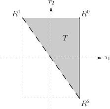
Figure 11: The image of $\boldsymbol{\tau_{2}}$ under the assumption that $\mathbf{m_{0}}$ lies on the segment between $\mathbf{m_{1}}$ and $\mathbf{m_{2}}$. In the gray region $T$ the map $\boldsymbol{\tau_{2}}$ is $2$–to–$1$. Along the horizontal and vertical sides of $T$ the map is $1$–to–$1,$ with the exception of the vertices $R^{1},R^{2}$, where the fibers of $\boldsymbol{\tau_{2}}$ are not finite. Finally, the dashed side of $T$ is not in Im($\boldsymbol{\tau_{2}}$).

The preimages of $\boldsymbol{\tau}\in\mbox{Im}(\boldsymbol{\tau_{2}})$ in the $x$–plane are

$$\mathbf{x}(\boldsymbol{\tau})=\pi(\mathbf{L_{0}}(\boldsymbol{\tau}))+\lambda\,\mathbf{v}(\boldsymbol{\tau}),$$

where $\lambda=\pm\|\mathbf{D_{10}}(\boldsymbol{\tau})\|\ \|\mathbf{D_{20}}(\boldsymbol{\tau})\|\ \|\mathbf{D_{21}}(\boldsymbol{\tau})\|/2d_{10}^{2}|k\tau_{1}-\tau_{2}|$ and $\pi$ is the projection onto the $x$–plane. Moreover, we have

$$\mathbf{D_{0}}(\pi(\mathbf{L_{0}}(\boldsymbol{\tau})))=\frac{\|\mathbf{D_{20}}(\boldsymbol{\tau})\|^{2}\tau_{1}-\|\mathbf{D_{10}}(\boldsymbol{\tau})\|^{2}k\tau_{2}}{2d_{10}^{2}(k\tau_{1}-\tau_{2})}\,\mathbf{d_{10}}.$$

In order to interpret the results, we notice that in the aligned configuration, the foci of $A_{1}(\boldsymbol{\tau}),A_{2}(\boldsymbol{\tau})$ belong to the line $r$, therefore the two level sets $A_{1}(\boldsymbol{\tau}),A_{2}(\boldsymbol{\tau})$ are both symmetrical with respect to $r$. We are in the $1$–to–$1$ situation if, and only if, the source $\mathbf{x}$ belongs to $r^{0}$, corresponding to $A_{1}(\boldsymbol{\tau}),A_{2}(\boldsymbol{\tau})$ tangentially intersecting at $\mathbf{x}$. In the general case, when $\boldsymbol{\tau}\in\mathring{T}$, the level sets meet at two distinct symmetrical points. This agrees with the classical statement that it is not possible to distinguish between symmetric configuration of the source, with respect to $r$, using a linear array of receivers.

The degenerate situation occurs for $\mathbf{x}\in r^{c}$, dual to $\boldsymbol{\tau}$ equal both to $(d_{10},{\rm sgn}(k)d_{20})$ and $(-d_{10},-{\rm sgn}(k)d_{20})$. In this case the localization of the source is totally unavailable, because the preimages contain infinitely many points of the $x$–plane. Finally, the points on the interior of the side $\tau_{2}-k\tau_{1}=0$ correspond to $A_{1}(\boldsymbol{\tau}),A_{2}(\boldsymbol{\tau})$ with parallel asymptotic lines and empty intersection.

8 The image of the complete TDOA map

In Section 2 we explained that the relation between $\boldsymbol{\tau_{2}}$ and $\boldsymbol{\tau_{2}^{*}}$ is given by the projection $p_{3}$ from the plane $\mathcal{H}\subset\mathbb{R}^{3}$ to $\mathbb{R}^{2}$ via the equality $\boldsymbol{\tau_{2}}=p_{3}\circ\boldsymbol{\tau_{2}^{*}}.$ As $p_{3}$ is invertible, it holds that $\boldsymbol{\tau_{2}^{*}}=p_{3}^{-1}\circ\boldsymbol{\tau_{2}}$ and consequently we have the following result:

Theorem 8.1

Im($\boldsymbol{\tau_{2}^{*}}$)=$p_{3}^{-1}$(Im($\boldsymbol{\tau_{2}}$)). More precisely, let $\boldsymbol{\tau^{*}}\in\mathcal{H}$, then $\boldsymbol{\tau_{2}^{*}}^{-1}({\boldsymbol{\tau^{*}}})=\boldsymbol{\tau_{2}}^{-1}({\boldsymbol{\tau}}),$ where $\boldsymbol{\tau}=p_{3}(\boldsymbol{\tau^{*}}).$

Theorem 8.1 allows us to give the explicit description of Im($\boldsymbol{\tau_{2}^{*}}$), thus reaching one of the main objectives we set ourselves in Section 2. We start by defining the relevant subsets of $\mathcal{H}$.

Definition 8.2

Assuming $0\leq i,j,k\leq 2$ distinct, in the $\tau^{*}$–space we set:

• $\mathcal{P}_{2}=\{\boldsymbol{\tau}^{*}\in\mathcal{H}\ |\ \|\mathbf{D_{ji}}(\boldsymbol{\tau}^{*})\|^{2}\geq 0\mbox{ for every }i,j\};$

• $\mathcal{F}_{k}^{+}=\{\boldsymbol{\tau}^{*}\in\mathcal{P}_{2}\ |\ \|\mathbf{D_{ji}}(\boldsymbol{\tau}^{*})\|^{2}=0,\langle\mathbf{D_{ji}}(\boldsymbol{\tau}^{*}),\mathbf{e_{3}}\rangle<0\};$

• $\mathcal{F}_{k}^{-}=\{\boldsymbol{\tau}^{*}\in\mathcal{P}_{2}\ |\ \|\mathbf{D_{ji}}(\boldsymbol{\tau}^{*})\|^{2}=0,\langle\mathbf{D_{ji}}(\boldsymbol{\tau}^{*}),\mathbf{e_{3}}\rangle>0\};$

• $\mathcal{E}_{k}=\{\boldsymbol{\tau}^{*}\in\mathcal{P}_{2}\ |\ \|\mathbf{D_{ik}}(\boldsymbol{\tau}^{*})\wedge\mathbf{D_{jk}}(\boldsymbol{\tau}^{*})\|^{2}=0\}.$

As the above definitions are stated using the exterior algebra formalism, for completeness we observe that $\mathcal{H}$ can also be described in similar terms:

$$\mathcal{H}=\{\boldsymbol{\tau}^{*}\in\mathbb{R}^{3}\ |\ \mathbf{D_{10}}(\boldsymbol{\tau}^{*})-\mathbf{D_{20}}(\boldsymbol{\tau}^{*})+\mathbf{D_{21}}(\boldsymbol{\tau}^{*})=\mathbf{0}\}$$

In Fig. 12 we show an example of Im($\boldsymbol{\tau_{2}^{*}}$) along with its projection Im($\boldsymbol{\tau_{2}}$).

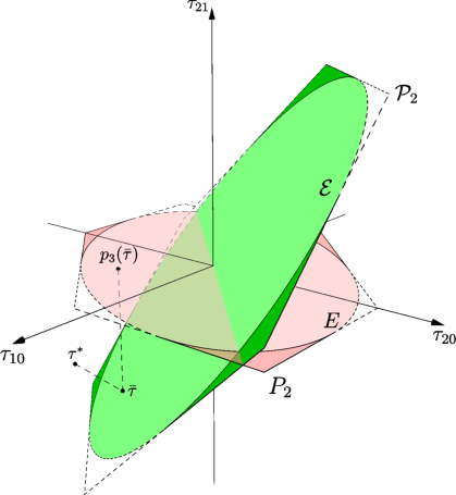
Figure 12: The image of $\boldsymbol{\tau_{2}^{*}}$ is the subset of $\mathcal{P}_{2}$ in green, while the image of $\boldsymbol{\tau_{2}}$ is the subset of $P_{2}$ in red. There is a 1–to–1 correspondence between Im($\boldsymbol{\tau_{2}^{*}}$) and Im($\boldsymbol{\tau_{2}}$) via the projection map $p_{3}$. In the lightly shaded regions, the TDOA maps are $1$–to–$1$, while in the more darkly shaded regions the maps are $2$–to–$1$. As explained in Section 10, three noisy TDOAs define a point $\boldsymbol{\tau^{*}}$ outside $\mathcal{P}_{2}$. The Maximum Likelihood Estimator computes the projection $\bar{\boldsymbol{\tau}}=p_{\mathcal{H}}(\boldsymbol{\tau^{*}})$ on $\mathcal{P}_{2}$, then the estimated source position is computed as $\bar{\mathbf{x}}=\boldsymbol{\tau_{2}^{*}}^{-1}(\bar{\boldsymbol{\tau}})=\boldsymbol{\tau_{2}}^{-1}(p_{3}(\bar{\boldsymbol{\tau}}))$.

As a consequence of Theorem 8.1, the structure of Im($\boldsymbol{\tau_{2}^{*}}$) turns out to be similar to that of Im($\boldsymbol{\tau_{2}}$), thus we can omit the proofs and go over the main facts about $\boldsymbol{\tau_{2}^{*}}$.

• $\boldsymbol{\tau_{2}^{*}}$ is a local diffeomorphism between the $x$–plane and $\mathcal{H},$ with the exception of the degeneracy locus $\cup_{i=0}^{2}(r_{i}^{-}\cup r_{i}^{+})$, as described in Theorem 3.2.

• $\mathcal{P}_{2}$ is the convex polygon given by $p_{3}^{-1}(P_{2})$, whose facets are $\mathcal{F}_{k}^{\pm}=p_{3}^{-1}({F_{k}^{\pm}})$. The image of $\boldsymbol{\tau_{2}^{*}}$ is a proper subset of $\mathcal{P}_{2}$ and, in particular, the image of the degeneracy locus is a subset of the facets.

• $\mathcal{E}_{k}$ does not depend on $k$. If the points $\mathbf{m_{0}}$, $\mathbf{m_{1}}$ and $\mathbf{m_{2}}$ are not aligned, then we have $\mathcal{E}_{k}=p_{3}^{-1}(E)$. Therefore, $\mathcal{E}_{k}$ is the unique ellipse that is tangent to each facet of the hexagon $\mathcal{P}_{2}$. The cardinality of each fiber of $\boldsymbol{\tau_{2}^{*}}$ is equal to that of the corresponding fiber of $\boldsymbol{\tau_{2}}$, as described in Theorem 6.16 and in Proposition 6.21.

• If the points $\mathbf{m_{0}},\mathbf{m_{1}},\mathbf{m_{2}}$ are aligned, then $\mathcal{E}_{k}$ is one of the diagonals of the quadrangle $\mathcal{P}_{2}$. The cardinality of each fiber of $\boldsymbol{\tau_{2}^{*}}$ is equal to that of the corresponding fiber of $\boldsymbol{\tau_{2}}$, as described in Theorem 7.5.

Remark 8.3

In the definition of $\boldsymbol{\tau_{2}^{*}}$ we notice a natural symmetry among the points $\mathbf{m_{0}}$, $\mathbf{m_{1}}$ and $\mathbf{m_{2}}$, which is lost in $\boldsymbol{\tau_{2}}$ as we elected $\mathbf{m_{0}}$ to be the reference microphone. As noticed in Section 2, by taking $p_{1}\circ\boldsymbol{\tau}_{2}^{*}$ or $p_{2}\circ\boldsymbol{\tau}_{2}^{*}$ we define different TDOA maps, with different reference microphones. Quite obviously, their properties are similar to those of $\boldsymbol{\tau_{2}}$ studied in Sections 6 and 7, in fact $p_{1}\circ p_{3}^{-1}$ and $p_{2}\circ p_{3}^{-1}$ are invertible maps between the images of the TDOA maps, factorizing on Im($\boldsymbol{\tau_{2}}^{*}$). Although such maps are, in fact, equivalent, some of their properties could be more or less difficult to check depending on the chosen reference point. For example, the lines $F_{0}^{\pm}$ become parallel to the reference axes when applying $p_{i}\circ p_{3}^{-1}$ for $i=1$ or $2$.

Remark 8.4

The previous remark implies that $p_{i}\circ p_{3}^{-1}$ sends the ellipse $E$ onto the ellipse associated to the TDOA map $p_{i}\circ\boldsymbol{\tau}_{2}^{*}$, but this does not happen for the cubic curve $C$. In fact, both the cubics associated to $p_{i}\circ\boldsymbol{\tau}_{2}^{*}$, $i=1,2$ do not contain (the transformations of) 4 of the 11 points characterizing $C$ in Proposition 6.12: $R^{0},R^{*},R^{0}_{1},R^{*}_{1}$. This, however, is not an issue for localization purposes, as the image of any TDOA map only depends on $C\cap E=E\cap P_{2}$.

9 Impact assessment

As anticipated in the Introduction, a complete characterization of the TDOA map constitutes an important building block for tackling a wide range of more general and challenging problems. For example, we could optimize sensor placement in terms of robustness against noise or measuring errors. More generally, we could embark into a statistical analysis of error propagation or consider more complex scenarios where the uncertainty lies with sensor synchronization or spatial sensor placement. While these general scenarios will be the topic of future contributions, in this Section we can already show an example of how to jointly use local and global analysis to shed light on the uncertainty in localisation problems.

A possible approach to the study of the accuracy of localization is based on the linearization of the TDOA model (see [20, 45]). Usually this analysis is pursued in a statistical context, but it essentially involves the analysis of the Jacobian matrix $J(\mathbf{x})$ of $\boldsymbol{\tau_{2}}$ and its determinant det$(J(\mathbf{x}))$. In the differential geometry interpretation, the absolute value of Jacobian determinant is the ratio between the areas of two corresponding infinitesimal regions in the $\tau$–plane and in the $x$–plane, under the action of the map $\boldsymbol{\tau_{2}}$. As a consequence, the quality of the localization is best in the regions of maximum of $|$det$(J(\mathbf{x}))|$, where the TDOAs are highly sensitive to differences of source position. This local analysis is equivalent, up to a costant factor, to that of the map $\boldsymbol{\tau_{2}^{*}}$. Starting from expression (10), in Fig. 13 we display the level sets of $|$det$(J(\mathbf{x}))|$ along with the geometric configuration of sensors and with the curves that we displayed earlier in Fig. 10.

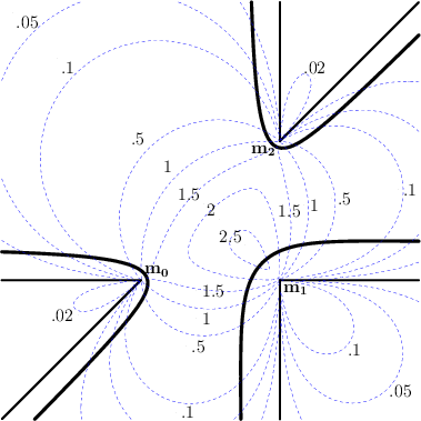
Figure 13: Level sets of the absolute value of the Jacobian determinant $|\det(J(\mathbf{x}))|$ of $\boldsymbol{\tau_{2}}$ (values are marked next to them). The picture also shows the bifurcation curve $\tilde{E}$ and the degeneracy locus $\det(J(\mathbf{x}))=0$, on the $x$–plane. Given the microphones in $\mathbf{m_{0}}=(0,0)$, $\mathbf{m_{1}}=(2,0)$, and $\mathbf{m_{2}}=(2,2)$, the best accuracy of the localization is obtained in the region that lies the closest to the center of the triangle. Notice that, although $\det(J(\mathbf{x}))$ is not affected by $\tilde{E}$, in the proximity to this curve the localization fails due to the global properties of $\boldsymbol{\tau_{2}}$.

Fig. 13 shows that the local error analysis does not take count of the global aspects of the localization. In particular, $|\det(J(\mathbf{x}))|$ becomes quite large in the proximity of the sensors. In these areas, however, localisation is not accurate because of their proximity to the bifurcation curve $\tilde{E}$ and the overlapping to the sets $\tilde{U}_{i}$. Having access to a complete global characterisation of the TDOA map allows us to predict this behaviour.

10 Conclusions and perspectives

In this manuscript we offered an exhaustive mathematical characterization of the TDOA map in the planar case of three receivers. We began with defining the non–algebraic complete TDOA map $\boldsymbol{\tau_{2}^{*}}$. We then derived a complete characterization of both Im$(\boldsymbol{\tau_{2}^{*}})\subset\mathbb{R}^{3}$ and the various preimage regions in the $x$–plane. We found that Im$(\boldsymbol{\tau_{2}^{*}})$ is a bounded subset of the plane $\mathcal{H}$ and, in particular, we showed that the image is contained in the convex polygon $\mathcal{P}_{2}$. We also described the subsets of the image in relation to the cardinality of the fibers, i.e. the loci where the TDOA map is $1$–to–$1$ or $2$–to–$1$, which provided a complete analysis of the a-priori identifiability problem. On the $x$–plane, we defined the degeneracy locus, where $\boldsymbol{\tau_{2}^{*}}$ is not a local diffeomorphism, and we described the sets where $\boldsymbol{\tau_{2}^{*}}$ is globally invertible and those where it is not.

We conducted our analysis using various mathematical tools, including multilinear algebra, the Minkowski space, algebraic and differential geometry. Indeed, these tools may seem too sophisticated for a problem as “simple” as that of TDOA-based localization. After all, this is a problem that, in the engineering literature, is commonly treated as consolidated or even taken for granted. As explained in the Introduction, however, the purpose of this work was twofold:

1. to derive analytically and in the most general sense what was preliminarily shown in a fully simulative fashion in [51], and to make the analysis valid for arbitrary sensor geometries;

2. to offer a complete characterisation of the TDOA map, to be applied to the solution of more general problems.

The first purpose was amply proven throughout the manuscript (Sections 2 to 8). What remains to be shown is how this analysis can pave the way to a deeper understanding of the localization problem in more general settings, such as in the presence of noisy measurements (propagation of uncertainty) or even in the presence of uncertainty in the sensor calibration and/or in their synchronization. An early discussion in this direction was offered in Section 9 where we described how errors propagate in a three-sensor setup based on local analysis and showed that, without a global perspective on the behaviour of the TDOA map we could be easily led to drawing wrong conclusions.

The authors are currently working on the extension to arbitrary distributions of sensors both in the plane and in the 3D Euclidean space, using similar techniques and notations. In particular, the model can be encoded as well in a TDOA map $\boldsymbol{\tau_{n}^{*}}$, whose image is a real surface and a real threefold, respectively. We expect the bifurcation locus and the $2$–to–$1$ regions to become thinner as the number of receivers in general position increase, although they do not immediately disappear (for example, in the planar case and $n=3,$ there are still curves in the $x$–plane where the localization is ambiguous). The precise description of $\boldsymbol{\tau_{n}^{*}}$ is needed also for the study of the localization with partially synchronized microphones. In fact, in this scenario not all TDOAs are available and, in our description, this is equivalent to considering some kind of projection of Im($\boldsymbol{\tau_{n}^{*}}$), just like the relationship between $\boldsymbol{\tau_{2}^{*}}$ and $\boldsymbol{\tau_{2}}$, explained in Sections 2 and 8.

In a near future we also want to pursue the study of the nonlinear statistical model, following a similar gradual approach to the one of this manuscript. Even in this respect, the knowledge of the noiseless measurements set Im($\boldsymbol{\tau_{n}^{*}}$) constitutes the starting point for any further advances on the study of the stochastic model. Roughly speaking, a vector of measurements $\boldsymbol{\tau}^{*}$ affected by errors corresponds to a point that lies close to the set Im($\boldsymbol{\tau_{n}^{*}}$) and the localization is a two-step procedure: we can first estimate $\bar{\boldsymbol{\tau}}\in\rm{Im}(\boldsymbol{\tau_{n}^{*}})$ from $\boldsymbol{\tau}^{*}$, then we evaluate the inverse map $\boldsymbol{\tau_{n}^{*}}^{-1}(\bar{\boldsymbol{\tau}})$.

We can give a real example of this process in the case of the complete TDOA model defined through the map $\boldsymbol{\tau_{2}^{*}}$. In a noisy scenario (e.g. with Gaussian errors), a set of three TDOAs gives a point $\boldsymbol{\tau^{*}}$ in the three dimensional $\tau^{*}$–space, that with probability 1 is not on the plane $\mathcal{H}$. A standard approach to obtain an estimation $\bar{\mathbf{x}}$ of the source position is through Maximum Likelihood Estimator (MLE). With respect to the discussion of the previous paragraph, it is well known that the estimated $\bar{\boldsymbol{\tau}}\in\rm{Im}(\boldsymbol{\tau_{2}^{*}})$ given by MLE is the orthogonal projection of $\boldsymbol{\tau^{*}}$ on the noiseless measurements set, i.e. the projection $p_{\mathcal{H}}(\boldsymbol{\tau^{*}})$ on $\mathcal{H}$ (see [42, 6] and Fig. 12) therefore $\bar{\mathbf{x}}=\boldsymbol{\tau_{2}^{*}}^{-1}(p_{\mathcal{H}}(\boldsymbol{\tau^{*}}))$.

A similar reasoning applies to the more complex case of $\boldsymbol{\tau_{n}^{*}}$. In particular, any estimator has a geometrical interpretation and the relative accuracy depends on the (non trivial) shape of Im($\boldsymbol{\tau_{n}^{*}}$). Possible techniques to be applied come from Information Geometry [6, 35], an approach that proved successful in similar situations and that is based on the careful description of Im($\boldsymbol{\tau_{n}^{*}}$). With this in mind, notice that our characterization of the TDOA model in algebraic geometry terms becomes instrumental for understanding and computing the MLE. Very recently, novel techniques have been developed and applied to to similar situations, in cases where scientific and engineering models are expressed as sets of real solutions to systems of polynomial equations (see, for example, [4, 25, 35]). The somewhat surprising fact that, although the TDOA map is not polynomial, all the loci involved in the analysis of $\boldsymbol{\tau_{2}^{*}}$ are algebraic or semi–algebraic, is a promising indicator of the effectiveness of this approach.

Appendix A The exterior algebra formalism

In this appendix, we recall the main definitions and some useful results about the exterior algebra of a real vector space. At the end, we analyze in full detail the two main examples that we use in the paper, namely the $2$–dimensional Euclidean case and the $3$–dimensional Minkowski one. The literature on the subject is wide and we mention [3] among the many possible references.

Let $V$ be a $n$–dimensional $\mathbb{R}$–vector space. Adopting a standard notation, $\wedge V$ is the exterior algebra of $V$ (hence, $\wedge^{k}V=0$ for each $k\geq n+1$ while $\wedge^{k}V$ has dimension ${n\choose k}$ for $k=0,\dots,n$). Roughly speaking, the symbol $\wedge$ is skew–commutative, and linear with respect to each factor. Hence, given the basis $(\mathbf{e_{1}},\dots,\mathbf{e_{n}})$ of $V,$ the reader can simply think at $\wedge^{k}V$ as the $\mathbb{R}$–vector space spanned by $\mathbf{e_{i_{1}}}\wedge\dots\wedge\mathbf{e_{i_{k}}}$ for $1\leq i_{1}<\dots<i_{k}\leq n.$

We choose a non–degenerate, symmetric bilinear form $b:V\times V\to\mathbb{R},$ and an orthonormal basis $B=(\mathbf{e_{1}},\dots,\mathbf{e_{n}})$ with respect to $b$, which means

$$b(\mathbf{e_{i}},\mathbf{e_{j}})=\left\{\begin{array}[]{cl}1&\mbox{ if }i=j=1,\dots,r,\\ -1&\mbox{ if }i=j=r+1,\dots,n,\\ 0&\mbox{ if }i\not=j.\end{array}\right.$$

The couple $(r,n-r)$ is the signature of $b.$ By setting $\langle\mathbf{u},\mathbf{v}\rangle=b(\mathbf{u},\mathbf{v})$ and $\parallel\mathbf{u}\parallel^{2}=b(\mathbf{u},\mathbf{u}),$ we can easily compute their expression in coordinates with respect to $B,$ and we have

$$\qquad\begin{array}[]{l}\langle\sum_{i=1}^{n}u_{i}\mathbf{e_{i}},\sum_{j=1}^{n}v_{i}\mathbf{e_{i}}\rangle=u_{1}v_{1}+\dots+u_{r}v_{r}-u_{r+1}v_{r+1}-\dots-u_{n}v_{n}\\ \\ \parallel\sum_{i=1}^{n}u_{i}\mathbf{e_{i}}\parallel^{2}=u_{1}^{2}+\dots+u_{r}^{2}-u_{r+1}^{2}-\dots-u_{n}^{2}\end{array}$$ (23)

The inner product in $\wedge^{k}V$ is defined by

$$\qquad\qquad\langle\mathbf{u_{1}}\wedge\dots\wedge\mathbf{u_{k}},\mathbf{v_{1}}\wedge\dots\wedge\mathbf{v_{k}}\rangle=\det\left(\begin{array}[]{ccc}\langle\mathbf{u_{1}},\mathbf{v_{1}}\rangle&\dots&\langle\mathbf{u_{1}},\mathbf{v_{k}}\rangle\\ \vdots&&\vdots\\ \langle\mathbf{u_{k}},\mathbf{v_{1}}\rangle&\dots&\langle\mathbf{u_{k}},\mathbf{v_{k}}\rangle\end{array}\right)$$ (24)

and extended by linearity. For example, $(\mathbf{e_{1}}\wedge\mathbf{e_{2}},\mathbf{e_{1}}\wedge\mathbf{e_{3}},\dots,\mathbf{e_{n-1}}\wedge\mathbf{e_{n}})$ is an orthonormal basis of $\wedge^{2}V,$ while $(\boldsymbol{\omega}=\mathbf{e_{1}}\wedge\dots\wedge\mathbf{e_{n}})$ is an orthonormal basis of $\wedge^{n}V$ with $\parallel\boldsymbol{\omega}\parallel^{2}=(-1)^{n-r}.$

Finally, from the choice of $\boldsymbol{\omega}$ as positive basis of $\wedge^{n}V,$ and from the fact that the natural concatenation of a $k$–form and a $(n-k)$–form gives a $n$–form, one recovers the classical Hodge $\ast$ operator $\mathbb{R}\to\wedge^{n}V$, $V\to\wedge^{n-1}V,\dots,\wedge^{n-1}V\to V$, and $\wedge^{n}V\to\mathbb{R},$ that are all isomorphisms.

Definition A.1

Given $\boldsymbol{\omega}\in\wedge^{n}V,\boldsymbol{\omega}\not=\mathbf{0},$ there exists a unique linear map $\ast:\wedge^{k}V\to\wedge^{n-k}V$ that verifies the condition

$$\mathbf{x}\wedge\ast\mathbf{y}=\langle\mathbf{x},\mathbf{y}\rangle\boldsymbol{\omega}$$

for every $\mathbf{x},\mathbf{y}\in\wedge^{k}V.$

Theorem A.2

The map $*:\wedge^{k}V\to\wedge^{n-k}V$ satisfies both $*\circ*=(-1)^{n-r+k(n-k)}{\rm id}_{\wedge^{k}V}$ and $\langle*\mathbf{x},*\mathbf{y}\rangle=(-1)^{n-r}\langle\mathbf{x},\mathbf{y}\rangle$ for every $\mathbf{x},\mathbf{y}$ in $\wedge^{k}V,$ and for any $k=0,\ldots,n$.

We now consider the dual space $V^{*}$ of $V$, i.e. the $\mathbb{R}$-vector space of the $\mathbb{R}$–linear maps from $V$ to $\mathbb{R}.$ Given the basis $(\mathbf{e_{1}},\dots,\mathbf{e_{n}})$ of $V,$ the dual space can be identified with the $n\times 1$ row matrices whose entries are the values that the map takes at $\mathbf{e_{i}},i=1,\dots,n.$

We use the form $b$ to construct an isomorphism between $V$ and $V^{*}$. Given $\mathbf{u}\in V$, we define $\mathbf{u}^{\flat}\in V^{*}$ by setting $\mathbf{u}^{\flat}(\mathbf{v})=\langle\mathbf{u},\mathbf{v}\rangle$. It is easy to prove that ${}^{\flat}:V\to V^{*}$ is an isomorphism, and so $B^{\flat}=(\mathbf{e_{1}}^{\flat},\dots,\mathbf{e_{n}}^{\flat})$ is a basis of $V^{*}.$ We want $V$ and $V^{*}$ to be isometric. Therefore we choose the non–degenerate, symmetric, bilinear form $b^{\flat}$ on $V^{*}$ as

$$b^{\flat}(\mathbf{u}^{\flat},\mathbf{v}^{\flat})=b(\mathbf{u},\mathbf{v})\qquad\mbox{ for every }\mathbf{u}^{\flat},\mathbf{v}^{\flat}\in V^{*}.$$

In such a way, $B^{\flat}$ is orthonormal with the same signature as $B$. We define ${}^{\sharp}:V^{*}\to V$ to be the inverse isomorphism of ${}^{\flat},$ i.e. $(\sum_{i=1}^{n}u_{i}\mathbf{e_{i}}^{\flat})^{\sharp}=\sum_{i=1}^{n}u_{i}\mathbf{e_{i}}.$ We can estend ^♭ and ^♯ to the associated exterior algebra $\wedge V^{*}$, obtaining the isomorphisms $\wedge^{k}V\to\wedge^{k}V^{*}$ and $\wedge^{k}V^{*}\to\wedge^{k}V:$

$$(\mathbf{u_{1}}\wedge\dots\wedge\mathbf{u_{k}})^{\flat}=\mathbf{u_{1}}^{\flat}\wedge\dots\wedge\mathbf{u_{k}}^{\flat}\quad\mbox{ and }\quad(\boldsymbol{\alpha_{1}}\wedge\dots\wedge\boldsymbol{\alpha_{k}})^{\sharp}=\boldsymbol{\alpha_{1}}^{\sharp}\wedge\dots\wedge\boldsymbol{\alpha_{k}}^{\sharp}.$$

As for $\wedge^{k}V$, we follow a similar procedure, and extend $b^{\flat}$ to $\wedge^{k}V^{*}$. Finally, after choosing $\boldsymbol{\omega}^{\flat}$ as positive basis of $\wedge^{n}V^{*}$, we define the Hodge $\ast$ operator on $\wedge^{k}V^{*}$, as

$$\ast(\mathbf{x})=\left(\ast(\mathbf{x}^{\sharp})\right)^{\flat}\qquad\mbox{ for each }\mathbf{x}\in\wedge^{k}V^{*}.$$

As last general topic, we consider the evaluation of a $k$–form in $\wedge^{k}V^{*}$ on $\mathbf{u}\in V.$ Such operation gives rise to the linear map $\mathbf{i}_{\mathbf{u}}:\wedge^{k}V^{*}\to\wedge^{k-1}V^{*}$ defined as

$$\qquad\qquad\mathbf{i}_{\mathbf{u}}(\boldsymbol{\alpha_{1}}\wedge\dots\wedge\boldsymbol{\alpha_{k}})=\sum_{i=1}^{k}(-1)^{i-1}\boldsymbol{\alpha_{i}}(\mathbf{u})\ \boldsymbol{\alpha_{1}}\wedge\dots\wedge\widehat{\boldsymbol{\alpha_{i}}}\wedge\dots\wedge\boldsymbol{\alpha_{k}}$$ (25)

where $\widehat{\boldsymbol{\alpha_{i}}}$ means that the item is missing.

A.1 The Euclidean vector space of dimension $2$

Let $V$ be a $2$–dimensional vector space on $\mathbb{R},$ let $b$ a non–degenerate bilinear form with signature $(2,0),$ and let $B=(\mathbf{e_{1}},\mathbf{e_{2}})$ be an orthonormal basis with respect to $b.$ Then, $\wedge^{k}V=0$ for $k\geq 3,$ and $\wedge^{2}V$ has dimension $1$ with $(\boldsymbol{\omega}=\mathbf{e_{1}}\wedge\mathbf{e_{2}})$ as orthonormal basis. On the natural bases, the Hodge operator is defined as:

$$\ast(1)=\boldsymbol{\omega},\ \ast(\mathbf{e_{1}})=\mathbf{e_{2}},\ \ast(\mathbf{e_{2}})=-\mathbf{e_{1}},\ \ast(\boldsymbol{\omega})=1.$$

Analogously, $V^{*}$ has dimension $2,$ with basis $(\mathbf{e_{1}}^{\flat},\mathbf{e_{2}}^{\flat}),$ where

$$\mathbf{e_{i}}^{\flat}(u_{1}\mathbf{e_{1}}+u_{2}\mathbf{e_{2}})=b(\mathbf{e_{i}},u_{1}\mathbf{e_{1}}+u_{2}\mathbf{e_{2}})=u_{i}\qquad\mbox{ for }i=1,2,$$

and

$$\ast(1)=\boldsymbol{\omega}^{\flat},\ \ast(\mathbf{e_{1}}^{\flat})=\mathbf{e_{2}}^{\flat},\ \ast(\mathbf{e_{2}}^{\flat})=-\mathbf{e_{1}}^{\flat},\ \ast(\boldsymbol{\omega}^{\flat})=1.$$

Proposition A.3

Let $\mathbf{u}=u_{1}\mathbf{e_{1}}+u_{2}\mathbf{e_{2}},\mathbf{v}=v_{1}\mathbf{e_{1}}+v_{2}\mathbf{e_{2}}\in V$ and $\mathbf{u}^{\flat}=u_{1}\mathbf{e_{1}}^{\flat}+u_{2}\mathbf{e_{2}}^{\flat},\mathbf{v}^{\flat}=v_{1}\mathbf{e_{1}}^{\flat}+v_{2}\mathbf{e_{2}}^{\flat}\in V^{*}.$ Then,

$$\ast(\mathbf{u}\wedge\mathbf{v})=\det\left(\begin{array}[]{cc}u_{1}&v_{1}\\ u_{2}&v_{2}\end{array}\right)\qquad\mbox{ and }\qquad\ast(\mathbf{u}^{\flat}\wedge\mathbf{v}^{\flat})=\det\left(\begin{array}[]{cc}u_{1}&u_{2}\\ v_{1}&v_{2}\end{array}\right).$$

We adopt the usual convention that the components of a vector in $V$ are written as columns, while the components of a vector in $V^{*}$ are written as rows. Of course, the images of the two $2$–form are equal because of the properties of the determinant of a matrix. The proof is an easy computation and we do not write the details.

A.2 The Minkowski vector space of dimension $3$

Let $V$ be a $3$–dimensional vector space on $\mathbb{R},$ let $b$ a non–degenerate bilinear form with signature $(2,1),$ and let $B=(\mathbf{e_{1}},\mathbf{e_{2}},\mathbf{e_{3}})$ be an orthonormal basis with respect to $b.$ Then, $\wedge^{k}V=0$ for $k\geq 4,$ and $\wedge^{2}V$ has dimension $3$ with $(\mathbf{e_{1}}\wedge\mathbf{e_{2}},\mathbf{e_{1}}\wedge\mathbf{e_{3}},\mathbf{e_{2}}\wedge\mathbf{e_{3}})$ as orthonormal basis with signature $(1,2),$ while $\wedge^{3}V$ has dimension $1$ and $(\boldsymbol{\omega}=\mathbf{e_{1}}\wedge\mathbf{e_{2}}\wedge\mathbf{e_{3}})$ is an orthonormal basis of this last space. On the natural bases the $\ast$ operator acts as follows:

$$\ast(1)=\boldsymbol{\omega},\ \ast(\boldsymbol{\omega})=-1,$$

$$\ast(\mathbf{e_{1}})=\mathbf{e_{2}}\wedge\mathbf{e_{3}},\ \ast(\mathbf{e_{2}})=-\mathbf{e_{1}}\wedge\mathbf{e_{3}},\ \ast(\mathbf{e_{3}})=-\mathbf{e_{1}}\wedge\mathbf{e_{2}},$$

$$\ast(\mathbf{e_{1}}\wedge\mathbf{e_{2}})=\mathbf{e_{3}},\ \ast(\mathbf{e_{1}}\wedge\mathbf{e_{3}})=\mathbf{e_{2}},\ \ast(\mathbf{e_{2}}\wedge\mathbf{e_{3}})=-\mathbf{e_{1}}.$$

As before, we compute the images of the elements of the bases of $\wedge^{k}V^{*}$ via the Hodge $\ast$ operator, and we get:

$$*(1)=\boldsymbol{\omega}^{\flat},*(\boldsymbol{\omega}^{\flat})=-1,$$

$$*(\mathbf{e_{1}}^{\flat})=\mathbf{e_{2}}^{\flat}\wedge\mathbf{e_{3}}^{\flat},*(\mathbf{e_{2}}^{\flat})=-\mathbf{e_{1}}^{\flat}\wedge\mathbf{e_{3}}^{\flat},*(\mathbf{e_{3}}^{\flat})=-\mathbf{e_{1}}^{\flat}\wedge\mathbf{e_{2}}^{\flat},$$

$$*(\mathbf{e_{1}}^{\flat}\wedge\mathbf{e_{2}}^{\flat})=\mathbf{e_{3}}^{\flat},*(\mathbf{e_{1}}^{\flat}\wedge\mathbf{e_{3}}^{\flat})=\mathbf{e_{2}}^{\flat},*(\mathbf{e_{2}}^{\flat}\wedge\mathbf{e_{3}}^{\flat})=-\mathbf{e_{1}}^{\flat}.$$

Now we state some results that we use in the body of the paper.

Lemma A.4

Let $\mathbf{u},\mathbf{v},\mathbf{w}\in V$ be linearly independent, so $\boldsymbol{\Omega}=\mathbf{u}\wedge\mathbf{v}\wedge\mathbf{w}\not=\mathbf{0}.$ Then,

$$\ast(\mathbf{u})=-\frac{1}{\ast(\boldsymbol{\Omega})}\left(\langle\mathbf{u},\mathbf{w}\rangle\mathbf{u}\wedge\mathbf{v}+\|\mathbf{u}\|^{2}\mathbf{v}\wedge\mathbf{w}+\langle\mathbf{u},\mathbf{v}\rangle\mathbf{w}\wedge\mathbf{u}\right)$$

and

$$\ast\left(\mathbf{u}\wedge\mathbf{v}\right)=-\frac{1}{\ast(\boldsymbol{\Omega})}\left(\langle\mathbf{u}\wedge\mathbf{v},\mathbf{v}\wedge\mathbf{w}\rangle\mathbf{u}+\langle\mathbf{u}\wedge\mathbf{v},\mathbf{w}\wedge\mathbf{u}\rangle\mathbf{v}+\|\mathbf{u}\wedge\mathbf{v}\|^{2}\mathbf{w}\right).$$

Proof. From the linear independence of $\mathbf{u}$, $\mathbf{v}$, and $\mathbf{w}$, it follows that $\mathbf{u}\wedge\mathbf{v},\mathbf{v}\wedge\mathbf{w},\mathbf{w}\wedge\mathbf{u}$ is a basis of $\wedge^{2}V$. Hence, there exist elements in $\mathbb{R}$ such that $\ast(\mathbf{u})=a\mathbf{u}\wedge\mathbf{v}+b\mathbf{v}\wedge\mathbf{w}+c\mathbf{w}\wedge\mathbf{u}$. From the definition of $\ast$ follows that $\mathbf{u}\wedge\ast(\mathbf{u})=\|\mathbf{u}\|^{2}\boldsymbol{\omega}$. By substituting the expression of $\ast(\mathbf{u})$, and using the properties of $\wedge$ we obtain $b\,\boldsymbol{\Omega}=\|\mathbf{u}\|^{2}\boldsymbol{\omega}$ or, equivalently, $b\ast(\boldsymbol{\Omega})=-\|\mathbf{u}\|^{2}$, which gives $b=-\|\mathbf{u}\|^{2}/\ast(\boldsymbol{\Omega})$. Through a similar computation we can derive $a$ and $c$, therefore the first claim follows. The second claim can be proven through the same arguments, therefore we can skip the details. $\square$

Lemma A.5

Let $\mathbf{u},\mathbf{v}\in V,$ and $\boldsymbol{\gamma}\in V^{*}.$ Then, $\boldsymbol{\gamma}(*(\mathbf{u}\wedge\mathbf{v}))=*(\mathbf{u}\wedge\mathbf{v}\wedge\boldsymbol{\gamma}^{\sharp}).$

Proof. We can verify the equality by using components with respect to $B,B^{\flat}$. $\square$

Corollary A.6

Let $\boldsymbol{\alpha},\boldsymbol{\beta}\in V^{*}$ be linearly independent. Then $\mathbf{i}_{\mathbf{u}}(\boldsymbol{\alpha}\wedge\boldsymbol{\beta})=\mathbf{0}$ if, and only if, $\mathbf{u}\in\mathcal{L}\left(\left(*(\boldsymbol{\alpha}\wedge\boldsymbol{\beta})\right)^{\sharp}\right),$ where $\mathcal{L}(\dots)$ is the subspace generated by the vectors in parenthesis.

Proof. Assume $\mathbf{u}=t\left(*(\boldsymbol{\alpha}\wedge\boldsymbol{\beta})\right)^{\sharp},$ for some $t\in\mathbb{R}.$ Then

$$\boldsymbol{\alpha}(\mathbf{u})=t\boldsymbol{\alpha}\left(\left(*(\boldsymbol{\alpha}\wedge\boldsymbol{\beta})\right)^{\sharp}\right)=*(\boldsymbol{\alpha}^{\sharp}\wedge\boldsymbol{\beta}^{\sharp}\wedge\boldsymbol{\alpha}^{\sharp})=0.$$

A similar argument proves that $\boldsymbol{\beta}(\mathbf{u})=0$. By definition, $\mathbf{i}_{\mathbf{u}}(\boldsymbol{\alpha}\wedge\boldsymbol{\beta})=\boldsymbol{\alpha}(\mathbf{u})\boldsymbol{\beta}-\boldsymbol{\beta}(\mathbf{u})\boldsymbol{\alpha}$ therefore the claim follows.
Conversely, assume that $\boldsymbol{\alpha}(\mathbf{u})\boldsymbol{\beta}-\boldsymbol{\beta}(\mathbf{u})\boldsymbol{\alpha}=\mathbf{0}$. Then $\boldsymbol{\alpha}(\mathbf{u})=\boldsymbol{\beta}(\mathbf{u})=0$ because $\boldsymbol{\alpha},\boldsymbol{\beta}$ are linearly independent. Hence, $\langle\boldsymbol{\alpha}^{\sharp},\mathbf{u}\rangle=\langle\boldsymbol{\beta}^{\sharp},\mathbf{u}\rangle=0$. This implies that $\mathbf{u}=t\left(*(\boldsymbol{\alpha}\wedge\boldsymbol{\beta})\right)^{\sharp}$ for some $t\in\mathbb{R}$, which completes the proof. $\square$

Lemma A.7

Let $\boldsymbol{\Theta}\in\wedge^{3}V^{*}$ be a non–zero $3$–form. Then, $\mathbf{i}_{\mathbf{u}}(\boldsymbol{\Theta})=\boldsymbol{\alpha}\wedge\boldsymbol{\beta}$ if, and only if, $\mathbf{u}=\frac{1}{*(\boldsymbol{\Theta})}\left(*(\boldsymbol{\alpha}\wedge\boldsymbol{\beta})\right)^{\sharp}.$

Proof. There exists $t\in\mathbb{R}$, $t\not=0$, such that $\boldsymbol{\Theta}=t\boldsymbol{\omega}^{\flat}$, therefore,

$$\mathbf{i}_{\mathbf{u}}(\boldsymbol{\Theta})=t\left(\mathbf{e_{1}}^{\flat}(\mathbf{u})\mathbf{e_{2}}^{\flat}\wedge\mathbf{e_{3}}^{\flat}-\mathbf{e_{2}}^{\flat}(\mathbf{u})\mathbf{e_{1}}^{\flat}\wedge\mathbf{e_{3}}^{\flat}+\mathbf{e_{3}}^{\flat}(\mathbf{u})\mathbf{e_{1}}^{\flat}\wedge\mathbf{e_{2}}^{\flat}\right)=\boldsymbol{\alpha}\wedge\boldsymbol{\beta}.$$

This implies

$$*(\boldsymbol{\alpha}\wedge\boldsymbol{\beta})=t\left(-\langle\mathbf{e_{1}},\mathbf{u}\rangle\mathbf{e_{1}}^{\flat}-\langle\mathbf{e_{2}},\mathbf{u}\rangle\mathbf{e_{2}}^{\flat}+\langle\mathbf{e_{3}},\mathbf{u}\rangle\mathbf{e_{3}}^{\flat}\right)=-t\mathbf{u}^{\flat}$$

and $\mathbf{u}=-\frac{1}{t}*(\boldsymbol{\alpha}\wedge\boldsymbol{\beta})^{\sharp}.$ Moreover, $*(\boldsymbol{\Theta})=t*\!(\boldsymbol{\omega}^{\flat})=-t,$ therefore one side of the claim follows. The converse is proven through a straightforward computation. $\square$

Appendix B A brief introduction to plane algebraic geometry

In this Appendix, we recall the main definitions and results concerning curves in the affine or projective plane.

B.1 Affine spaces and algebraic subsets

Definition B.1

Let $\mathbb{K}$ be a field and let $V$ be a $\mathbb{K}$–vector space. Let $\Sigma$ be a non–empty set. A map $\phi:\Sigma\times\Sigma\to V$ that verifies

• $\phi(A,B)+\phi(B,C)=\phi(A,C)$ for every $A,B,C\in\Sigma$

• $\phi_{A}:\Sigma\to V$ defined as $\phi_{A}(X)=\phi(A,X)$ is $1$–to–$1$ for every $A\in\Sigma$

is an affine structure on $\Sigma,$ and the couple $(\Sigma,\phi)$ is called affine space and named $\mathbb{A}(V).$

The main example we use is the following: let $\Sigma=V,$ and define $\phi(\mathbf{u},\mathbf{v})=\mathbf{v}-\mathbf{u}.$ $\phi$ is an affine structure on $V$ and so we get the affine space $\mathbb{A}(V).$ If $\dim(V)=n,$ we say that $\mathbb{A}(V)$ has dimension $n,$ as well. The advantage to have an affine structure on a set of points is that we can easily define the coordinates of the points.

Definition B.2

Let $\mathbb{A}(V)$ be an affine space of dimension $n.$ A reference frame is a couple $\mathcal{R}=(O,B),$ where $O$ is a point, and $B=(\mathbf{v_{1}},\dots,\mathbf{v_{n}})$ is a basis of $V.$ Given $P\in\mathbb{A}(V),$ its coordinates in the frame $\mathcal{R}$ are the components of $\phi(O,P)$ with respect to $B.$

Thanks to the properties of the affine structure, once $\mathcal{R}$ is given, there is a $1$–to–$1$ correspondence between points in $\mathbb{A}(V)$ and elements in $\mathbb{K}^{n}.$ So, usually, the two spaces are identified. When this happens, one denotes $\mathbb{K}^{n}$ as $\mathbb{A}^{n}_{\mathbb{K}}$. We remark that the identification imply the choice of the reference frame, and so some care has to be taken if one works with more than one reference frame.

If $\mathbb{K}=\mathbb{R},$ and $V$ is an Euclidean vector space, then $\mathbb{A}(V)$ is referred to as Euclidean space, and indicated with $\mathbb{E}(V),$ or $\mathbb{E}^{n}$ emphasizing just the dimension of $V.$ In this setting, the set–theoretical equality between $\mathbb{E}^{n}$ and $\mathbb{A}^{n}_{\mathbb{R}}$ is evident. However, if one switches from $\mathbb{E}^{n}$ to $\mathbb{A}^{n}_{\mathbb{R}},$ then one is not allowed to use distances and angles.

Another standard construction is the following. Given the real vector space $V,$ one can consider the complex vector space $\bar{V}=\mathbb{C}\otimes_{\mathbb{R}}V.$ Roughly speaking, we allow complex numbers to multiply the vectors of $V.$ As example of the previous construction, we remark that $\mathbb{C}^{n}=\mathbb{C}\otimes_{\mathbb{R}}\mathbb{R}^{n}.$ It holds $\dim_{\mathbb{C}}\bar{V}=\dim_{\mathbb{R}}V,$ and $\dim_{\mathbb{R}}\bar{V}=2\dim_{\mathbb{R}}V.$ Of corse, we have a set–theoretical inclusion $V\subset\bar{V},$ that is not a linear map. The inclusion of vector spaces provides an inclusion of the corresponding affine spaces, that can be written as $\mathbb{A}^{n}_{\mathbb{R}}\subset\mathbb{A}^{n}_{\mathbb{C}},$ up to the choice of a reference frame with the same origin $O\in\mathbb{A}^{n}_{\mathbb{R}},$ and the same basis $B\subset V$ both for $V$ and for $\bar{V}$.

In the paper, we mainly use the affine space with $n=2,$ namely the affine plane. The geometrical objects in $\mathbb{A}^{2}_{\mathbb{K}}$ that are studied in the algebraic geometry framework are (algebraic) curves and their intersections. We recall the definition of algebraic curve.

Definition B.3

Let $f_{1},\dots,f_{r}\in\mathbb{K}[x,y]$ be polynomials. The vanishing locus $V(f_{1},\dots,f_{r})$ of the given polynomials is

$$V(f_{1},\dots,f_{r})=\{P\in\mathbb{A}^{2}_{\mathbb{K}}\ |\ f_{i}(P)=0\mbox{ for every }i=1,\dots,r\}.$$

The evaluation of a polynomial $f$ at $P,f(P),$ simply consists in substituting the coordinates of $P$ in the expression of $f.$

Definition B.4

A non–empty subset $C\subset\mathbb{A}^{2}_{\mathbb{K}}$ is an algebraic curve if there exists a polynomial $f\in\mathbb{K}[x,y]$ of degree $\geq 1$ such that $C=V(f).$

We get a line when the degree of $f$ is $1,$ a conic when the degree of $f$ is $2.$ From degree $3$ on, a curve is named according to the degree of $f,$ e.g. there are cubic curves, quartic ones, and so on.

The advantage of considering curves in $\mathbb{A}^{2}_{\mathbb{C}}$ is that some unpleasant phenomenon do not happen: the vanishing locus of $x^{2}+y^{2}$ is a single point in $\mathbb{A}^{2}_{\mathbb{R}}$ and a couple of lines in $\mathbb{A}^{2}_{\mathbb{C}},$ the vanishing locus of $x^{2}+y^{2}+1$ is empty in $\mathbb{A}^{2}_{\mathbb{R}},$ and a conic in $\mathbb{A}^{2}_{\mathbb{C}}.$

In greater generality, we can consider algebraic subsets.

Definition B.5

A subset $X\subset\mathbb{A}^{2}_{\mathbb{K}}$ is algebraic if there exist $f_{1},\dots,f_{r}\in\mathbb{K}[x,y]$ such that $X=V(f_{1},\dots,f_{r}).$

For example, the intersection of the curves $C_{i}=V(f_{i}),i=1,\dots,r,$ is the algebraic set $X=V(f_{1},\dots,f_{r}).$ It is possible to prove that algebraic sets are the closed sets of a topology, the Zariski topology, on $\mathbb{A}^{2}_{\mathbb{K}}.$

B.2 Projective spaces and algebraic subsets

Roughly speaking, the points of a projective space are the $1$–dimensional subspaces of a vector space. Hence, we have to identify all the vectors belonging to the same subspace. The mathematical machinery is the following one.

Definition B.6

Let $V$ be a $n+1$–dimensional vector space over the ground field $\mathbb{K}.$ We define the relation $\sim$ in $V\setminus\{\mathbf{0}\}$ as

$$\mathbf{u}\sim\mathbf{v}\quad\mbox{ if there exists }t\in\mathbb{K},t\not=0,\mbox{ such that }\mathbf{u}=t\mathbf{v}.$$

It is easy to check the following.

Proposition B.7

$\sim$ is an equivalence relation.

Definition B.8

The projective space of dimension $n$ over $V$ is the set of equivalence classes of $V\setminus\{\mathbf{0}\}$ modulo $\sim,$ that is to say,

$$\mathbb{P}(V)=(V\setminus\{\mathbf{0}\})/\sim.$$

As for the affine space, we define a reference frame in the projective space.

Definition B.9

Let $\mathbb{P}(V)$ be a projective space of dimension $n.$ A reference frame is $\mathcal{R}=(B),$ where $B=(\mathbf{v_{0}},\dots,\mathbf{v_{n}})$ is a basis of $V.$ Given $P\in\mathbb{P}(V),$ its homogeneous coordinates with respect to $\mathcal{R}$ are the components of $\mathbf{v}\in P$ with respect to $B,$ and we set $P=(x_{0}:\dots:x_{n}).$

The homogeneous coordinates of a point $P\in\mathbb{P}(V)$ are not unique. In fact, if $\mathbf{v}\in P,$ then $P$ contains also $t\mathbf{v}$ for every $t\in\mathbb{K},$ $t\not=0.$ The components of $t\mathbf{v}$ are the ones of $\mathbf{v}$ times $t,$ and so the homogeneous coordinates of a point are unique up to a scalar factor, i.e. if $(x_{0}:\dots:x_{n})$ are the homogeneous coordinates of $P,$ then also $(tx_{0}:\dots:tx_{n})$ are so, for every $t\not=0.$

A first property is the following one.

Proposition B.10

Let $V$ be a real vector space of dimension $n+1.$ Then

$$\mathbb{P}^{2}(V)\subset\mathbb{P}^{2}(\bar{V}=\mathbb{C}\otimes_{\mathbb{R}}V).$$

Proof. From the definition of $\bar{V},$ it follows that vectors that are proportional in $V$ are proportional also in $\bar{V},$ and so there is a natural way to identify a point $P\in\mathbb{P}(V)$ with a point in $\mathbb{P}(\bar{V}).$ This identification gives an inclusion. We remark that the two spaces are not equal for $n\geq 1.$ $\square$

Hence, we restrict to $\mathbb{P}(V)$ where $V$ is a vector space over the complex field and we stress the properties that behave differently in a projective space over a real vector space. Moreover, once a reference frame is given, we identify the points with their homogeneous coordinates. In this case, we simply write $\mathbb{P}^{n}_{\mathbb{C}}$ or $\mathbb{P}^{n}_{\mathbb{R}}$ to stress the dimension and the ground field. Motivated again from the case considered in the paper, we focus on the projective space of dimension $2,$ i.e. on the projective plane $\mathbb{P}^{2}_{\mathbb{C}}.$

In the projective setting, the polynomial to be considered are the homogeneous ones. In fact, due to the construction of the homogeneous coordinates, the evaluation of a polynomial at a points is in general a meaningless concept. However, it is meaningful to check if a polynomial vanishes at a projective point $P.$

Proposition B.11

Let $f\in\mathbb{K}[x_{0},x_{1},x_{2}]$ be equal to $f=f_{0}+f_{1}+\dots+f_{d}$ where $f_{i}$ is homogeneous of degree $i.$ Let $P\in\mathbb{P}^{2}_{\mathbb{K}}$ be the point with homogeneous coordinates $(x_{0}:x_{1}:x_{2}).$ Then, $f(P)=0$ if, and only if, $f_{i}(P)=0$ for each $i$.

Proof. We have $f(P)=f(x_{0}:x_{1}:x_{2})=f_{0}(x_{0}:x_{1}:x_{2})+f_{1}(x_{0}:x_{1}:x_{2})+\dots+f_{d}(x_{0}:x_{1}:x_{2}).$ The point $P,$ however, is represented also from the coordinates $(tx_{0}:tx_{1}:tx_{2})$ for every $t\not=0,$ and so we have $f(tx_{0}:tx_{1}:tx_{2})=f_{0}(tx_{0}:tx_{1}:tx_{2})+f_{1}(tx_{0}:tx_{1}:tx_{2})+\dots+f_{d}(tx_{0}:tx_{1}:tx_{2})=f_{0}(x_{0}:x_{1}:x_{2})+tf_{1}(x_{0}:x_{1}:x_{2})+\dots+t^{d}f_{d}(x_{0}:x_{1}:x_{2}).$ So, if $\mathbb{K}$ contains infinitely many elements, then $f_{i}(x_{0}:x_{1}:x_{2})=0$ for every $i=0,\dots,d.$ $\square$

This proposition justifies the fact that we restrict to homogeneous polynomials.

Definition B.12

Let $f_{1},\dots,f_{r}\in\mathbb{K}[x_{0},x_{1},x_{2}]$ be homogeneous polynomials. Then, their vanishing locus is

$$V(f_{1},\dots,f_{r})=\{P\in\mathbb{P}^{2}_{\mathbb{K}}\ |\ f_{i}(P)=0\mbox{ for every }i=1,\dots,r\}.$$

We are now ready to define the projective algebraic sets, and projective curves in particular.

Definition B.13

A non–empty subset $C\subset\mathbb{P}^{2}_{\mathbb{K}}$ is a projective plane curve if there exists a homogeneous polynomial $f$ such that $C=V(f).$
A subset $X\subseteq\mathbb{P}^{2}_{\mathbb{K}}$ is a projective algebraic set if there exist homogeneous polynomials $f_{1},\dots,f_{r}$ such that $X=V(f_{1},\dots,f_{r}).$

As in the case of the affine plane, it is possible to prove that the projective algebraic sets are the closed sets of a topology, the Zariski topology, on the projective plane. A line in $\mathbb{P}^{2}_{\mathbb{K}}$ is the vanishing locus of a degree $1$ homogeneous polynomial, a conic is the vanishing locus of a degree $2$ homogeneous polynomial, and so on.

As further step, we show that it is possible to include the affine plane in the projective one, as an open subset.

Proposition B.14

Let $H_{0}=V(x_{0})\subset\mathbb{P}^{2}_{\mathbb{K}}$ be a line, and let $U_{0}$ be the open complement of $H_{0}.$ Then, $U_{0}$ can be identified with the affine plane, and the identification preserves the algebraic sets.

Proof. Let $P=(x_{0}:x_{1}:x_{2})\in U_{0}.$ From the definition of $U_{0},$ it follows that $x_{0}\not=0,$ and so we can take $(1:x_{1}/x_{0}:x_{2}/x_{0})$ as the homogeneous coordinates of $P.$ If we set $x=x_{1}/x_{0},y=x_{2}/x_{0},$ then we can identify $P$ with the point $Q\in\mathbb{A}^{2}_{\mathbb{K}}$ whose coordinates are $(x,y).$ Conversely, each point $Q(x,y)\in\mathbb{A}^{2}_{\mathbb{K}}$ can be identified with the point $P\in U_{0}$ whose homogeneous coordinates are $(1:x:y).$ Hence, there is a $1$–to–$1$ correspondence between $U_{0}$ and $\mathbb{A}^{2}_{\mathbb{K}}.$ To prove the remaining part of the statement, we start considering curves. So, let $C\subset\mathbb{P}^{2}_{\mathbb{K}}$ be a curve different from $H_{0},$ and let $f(x_{0},x_{1},x_{2})\in\mathbb{K}[x_{0},x_{1},x_{2}]$ be a homogeneous polynomial such that $C=V(f).$ Let $g(x,y)=f(1,x,y)\in\mathbb{K}[x,y],$ and let $D\subset\mathbb{A}^{2}_{\mathbb{K}}$ be the affine curve it defines. Then, the previous correspondence maps the points in $C\cap U_{0}$ to points in $D,$ and conversely. So a curve in the projective plane is transformed in a curve in the affine plane. Conversely, let $D=V(g)$ be a curve in $\mathbb{A}^{2}_{\mathbb{K}},$ with $g\in\mathbb{K}[x,y].$ Let $d$ be the degree of $g,$ and let $f(x_{0},x_{1},x_{2})=x_{0}^{d}g(x_{1}/x_{0},x_{2}/x_{0}).$ It is easy to check that $f\in\mathbb{K}[x_{0},x_{1},x_{2}]$ is a degree $d$ homogeneous polynomial. Let $C=V(f)$ be the corresponding curve in the projective plane. Then, it is straightforward to prove that the points of $D$ are mapped to points in $C\cap U_{0}.$ As the algebraic sets are union of finitely many curves or intersection of curves, the proof is complete, because it holds on curves. $\square$

Notice that a consequence of the previous proof is that the complement of whatever line in $\mathbb{P}^{2}_{\mathbb{K}}$ is an affine plane. Conversely, the projective plane is the union of an affine plane and a projective line. The points of the projective line are called ideal points of the affine plane and are thought to as directions of the lines in the affine plane.

From now on, we deal with the geometry of algebraic sets in the projective plane $\mathbb{P}^{2}_{\mathbb{C}}$ because we have the chains of inclusions

$$\mathbb{E}^{2}=\mathbb{A}^{2}_{\mathbb{R}}\subset\mathbb{A}^{2}_{\mathbb{C}}\subset\mathbb{P}^{2}_{\mathbb{C}}\qquad\mbox{ and }\qquad\mathbb{E}^{2}=\mathbb{A}^{2}_{\mathbb{R}}\subset\mathbb{P}^{2}_{\mathbb{R}}\subset\mathbb{P}^{2}_{\mathbb{C}},$$

and we underline the problems when restricting to smaller ambient spaces.

B.3 Intersection of curves and singular points

A line $L$ in $\mathbb{P}^{2}_{\mathbb{C}}$ is the vanishing locus of a linear homogeneous equation $a_{0}x_{0}+a_{1}x_{1}+a_{2}x_{2}=0,$ and so it has parametric equation $x_{i}=b_{i}s+c_{i}t,s,t\in\mathbb{C},i=0,1,2.$ Given a curve $C=V(f),$ the intersection $L\cap C$ is given by solving the equation $f(b_{0}s+c_{0}t,\dots,b_{2}s+c_{2}t)=F(s,t)$ homogeneous of the same degree of $f.$ Hence, we have proved

Proposition B.15

A line $L$ intersects a degree $d$ curve $C$ at exactly $d$ points, up to count each point with its multiplicity.

Proof. The Fundamental Theorem of Algebra states that a degree $d$ equation in one variable has exactly $d$ roots over $\mathbb{C},$ up to count each root with its multiplicity. We can apply it to $F(1,t),$ after computing the largest power of $s$ that divides $F.$ $\square$

Of course, when restricting to $\mathbb{P}^{2}_{\mathbb{R}},$ the complex roots do not give contribution, and so a line meets a degree $d$ curve in at most $d$ points, up to count each one of them with multiplicity. When considering the intersection in $\mathbb{A}^{2}_{\mathbb{C}},$ the roots that correspond to ideal points give no contribution, and so again a line meets a degree $d$ curve in at most $d$ points. When restricting to $\mathbb{A}^{2}_{\mathbb{R}},$ one has to take care of both problems. As an example, we consider the conic $C=V(x_{1}^{2}-x_{0}x_{2})\subset\mathbb{P}^{2}_{\mathbb{C}},$ and the line $L_{1}=V(x_{0}+x_{2}).$ They meet at $A_{1}(i:1:-i)$ and $B_{1}(-i:1:i)$ where $i^{2}=-1.$ So, $C\cap L_{1}$ is empty, when the intersection is considered in $\mathbb{P}^{2}_{\mathbb{R}}.$ If we consider the line $L_{2}=V(x_{0}-x_{1}),$ the intersection of $C$ and $L_{2}$ consists of the points $A_{2}(0:0:1)$ and $B_{2}(1:1:1).$ Let $\mathbb{A}^{2}_{\mathbb{C}}$ be identified with $U_{1}$ complement of the line $H_{1}=V(x_{1}).$ Then the conic $C$ (the line $L_{2},$ respectively) has equation $xy-1=0$ ($x=1,$ respectively). The intersection contains the point $(1,1),$ only. In fact, $A_{2}$ is an ideal point for the identification of the affine plane with $U_{1}.$

The previous result can be generalized to the intersection of two curves of arbitrary degree.

Theorem B.16 (Bézout’s Theorem)

Let $C,C^{\prime}$ be projective plane curves of degree $d$ and $d^{\prime},$ respectively. If $C$ and $C^{\prime}$ have a finite number of common points, then there are exactly $dd^{\prime}$ intersection points, up to count them with their multiplicity.

The proof of Bézout’s Theorem can be found in [29, Ch.I, Corollary 7.8], and goes beyond the scopes of this introduction.

Now, we can define a smooth point on a curve.

Definition B.17

Let $C\subset\mathbb{P}^{2}_{\mathbb{C}}$ be a curve and let $P\in C$ be a point. $P$ is a smooth point of $C$ if there exists a line $L$ containing $P$ that intersects $C$ at $P$ with multiplicity $1.$ A curve $C$ whose points are all smooth is said to be smooth, singular otherwise.

The property is local, so we can reduce to an affine plane, by taking the complement of a line that do not contain $P.$ Moreover, we choose a reference frame in such affine plane so that $P$ is the origin. Hence, $C=V(f)$ for a suitable $f\in\mathbb{K}[x,y],$ with $f(0,0)=0.$ The lines through the origin have parametric equation $x=lt,y=mt,$ and the intersection between $C$ and one of such line is described by $f(lt,mt)=0.$ By McLaurin expansion, we have $0=(lf_{x}(0,0)+mf_{y}(0,0))t+$ higher degree terms. Hence, $P$ is smooth if there exists $l,m$ such that $lf_{x}(0,0)+mf_{y}(0,0)\not=0,$ or equivalently, the gradient $\nabla f(0,0)$ is not zero. We have then proved

Proposition B.18

A point $P\in C=V(f)$ is smooth for $C$ if $\nabla f(P)\not=\mathbf{0},$ where $f$ is a homogeneous polynomial that defines $C.$

Proposition B.18 allows us to prove that the singular locus $\mbox{Sing}(C)$ of $C=V(f)$ is algebraic and it holds $\mbox{Sing}(C)=V(f,f_{x_{0}},f_{x_{1}},f_{x_{2}}).$ Thanks to Euler formula for homogeneous functions

$$\qquad dF(x_{0},x_{1},x_{2})=x_{0}F_{x_{0}}(x_{0},x_{1},x_{2})+x_{1}F_{x_{1}}(x_{0},x_{1},x_{2})+x_{2}F_{x_{2}}(x_{0},x_{1},x_{2})$$ (26)

where $d$ is the degree of $F,$ we have that $\mbox{Sing}(C)=V(f_{x_{0}},f_{x_{1}},f_{x_{2}}).$ In the affine plane, if $C=V(f),$ we have $\mbox{Sing}(C)=V(f,f_{x},f_{y}).$

Also if intuition suggests that the singular points on a curve are finitely many special points, there are examples of curves with a subcurve of singular points. For example, consider the curve $C=V(x_{0}x_{1}^{2})$ in the projective plane $\mathbb{P}^{2}_{\mathbb{R}}.$ Then, $\mbox{Sing}(C)=V(2x_{0}x_{1},x_{1}^{2})=V(x_{1}).$ Hence, $C$ has the line $V(x_{1})$ as its singular locus. The curve $C$ is the union of the line $V(x_{0})$ and of the conic $V(x_{1}^{2}).$ The conic, however, is a double line (twice the line $V(x_{1})$), and so the singular locus of $C$ is equal to the double line. This phenomenon can be easily generalized. Before giving the definitions on curves to handle it, we recall some properties of polynomials. We state them for polynomials in two variables but they can be extended without effort to homogeneous polynomials in $3$ variables.

Definition B.19

A polynomial $f\in\mathbb{K}[x,y]$ is irreducible if it cannot be written as product of two non–constant polynomials.

Theorem B.20

Every polynomial $f\in\mathbb{K}[x,y]$ can be written as product of powers of irreducible polynomials, in a unique way, up to some non–zero constant.

Now, we translate the previous results in geometrical terms.

Definition B.21

A curve $C$ is

1. reduced and irreducible if $C=V(f)$ with $f$ irreducible;

2. irreducible and non–reduced if $C=V(f^{m})$ with $f$ irreducible and $m\geq 2;$

3. reduced, non–irreducible if $C=V(f_{1}\cdots f_{r})$ with $f_{i}$ irreducible for every $i;$

4. non–reduced and non–irreducible if $C=V(f_{1}^{m_{1}}\cdots f_{r}^{m_{r}})$ with $f_{i}$ irreducible and $m_{1}+\dots+m_{r}\geq r+1.$

Going back to the study of the singular locus of a curve, we have the following result.

Theorem B.22

The singular points of a curve $C$ are finitely many, or $C$ is smooth if and only if $C$ is reduced. Moreover, if $C$ is reduced and irreducible (reduced, respectively), there are at most $\left(\begin{array}[]{c}d-1\\ 2\end{array}\right)$ ($\left(\begin{array}[]{c}d\\ 2\end{array}\right),$ respectively) singular points on $C,$ where $d$ is the degree of $C.$

For example, a reduced and irreducible conic is smooth, while a reduced non–irreducible conic has exactly one singular point (the point where the two lines, whose union is the conic, meet). Furthermore, a reduced and irreducible cubic can have at most one singular point, a reduced and irreducible quartic curve can have at most $3$ singular points, and so on.

A notion, apparently non related to the singular locus of a curve, is the rationality of a curve.

Definition B.23

A curve $C=V(f)\subset\mathbb{P}^{2}_{\mathbb{C}}$ is rational if there exist $g_{0}(s,t),g_{1}(s,t),g_{2}(s,t)\in\mathbb{C}[s,t],$ homogeneous of degree equal to the one of $f,$ and without common factors of positive degree, such that $f(g_{0},g_{1},g_{2})$ is identically zero.

A rational curve is then a curve whose points have coordinates that can be expressed via the parameter functions $g_{i}(s,t),i=0,1,2.$ It is possible to prove that a reduced irreducible curve is rational if it has as much singular points as its degree allows. E.g., smooth conic, cubic with one singular point, quartic with three singular points, quintic with $6$ singular points, are all examples of rational curves. From one hand, more than the number of singular points, the rationality depends on the kind of singularities of the curve itself, on the other hand, a deeper study of the singular points of a curve goes further the scope of this introduction, and so we do not go on along these lines.

B.4 Dual projective plane

As explained earlier, a line in the projective plane is the vanishing locus of a non–zero degree $1$ homogeneous polynomial $a_{0}x_{0}+a_{1}x_{1}+a_{2}x_{2}=0.$ The coefficients $a_{0},a_{1},a_{2}$ are defined up to a scalar. In fact, for each $k\not=0,$ $(ka_{0})x_{0}+(ka_{1})x_{1}+(ka_{2})x_{2}=0$ defines the same line as the previous equation. Hence, the coefficients can be interpreted as points of a projective plane.

Definition B.24

Given the projective plane $\mathbb{P}(V),$ the dual plane is defined as $\mathbb{P}(V^{*}),$ where $V^{*}$ is the dual vector space of $V.$ Once a reference frame $\mathcal{R}=(B)$ is given in $\mathbb{P}(V),$ the dual basis $B^{*}$ defines the dual reference frame $\mathcal{R}^{*}$ in $\mathbb{P}(V^{*}).$ With this in mind, we set $\check{\mathbb{P}}^{2}_{\mathbb{K}}=\mathbb{P}(V^{*}),$ and the points of $\check{\mathbb{P}}^{2}_{\mathbb{K}}$ are the coefficients of the lines of $\mathbb{P}^{2}_{\mathbb{K}},$ or the lines of $\mathbb{P}^{2}_{\mathbb{K}},$ for short.

As $(V^{*})^{*}\cong V,$ the dual of the dual projective plane in the initial one. We can now define the dual curve.

Definition B.25

Let $C\subset\mathbb{P}^{2}_{\mathbb{K}}$ be a reduced and irreducible curve. The dual curve $\check{C}\subset\check{\mathbb{P}}^{2}_{\mathbb{K}}$ is the unique algebraic curve that contains the tangent lines at the points of $C.$

Assume that $C$ is smooth of degree $d.$ Then, $\check{C}$ has degree $d(d-1).$ We can assume $\mathbb{K}=\mathbb{C}$ because the degree does not depend on the ground field. A line in $\check{\mathbb{P}}^{2}_{\mathbb{C}}$ is a point in $\mathbb{P}^{2}_{\mathbb{C}}.$ Hence, we have to compute how many tangent lines to $C$ pass through the same point $A(x_{0}^{A}:x_{1}^{A}:x_{2}^{a})$ in $\mathbb{P}^{2}_{\mathbb{C}}.$ A tangent line contains $A$ if, and only if, $x_{0}^{A}f_{x_{0}}+x_{1}^{A}f_{x_{1}}+x_{2}^{A}f_{x_{2}}=0.$ This last curve has degree $d-1$ and is called the polar curve to $C$ with respect to the pole $A.$ The intersection points of $C$ and the polar curve are $d(d-1)$ by Bézout Theorem, and so the degree of $\check{C}$ is $d(d-1),$ as claimed.

Proposition B.26

Let $C$ be a smooth curve. Then, $C$ and $\check{C}$ have the same degree if and only if $C$ is a conic.

Proof. The solutions of the equation $d(d-1)=d$ are $d=0$ and $d=2,$ and $d=0$ cannot be accepted. $\square$

B.5 Hilbert function and the geometry of a set of points

Definition B.27

Let $X\subset\mathbb{P}^{2}_{\mathbb{K}}$ be an algebraic set. We set

$$I_{X}=\{f\in\mathbb{K}[x_{0},x_{1},x_{2}]\ |\ f\mbox{ is homogeneous and }f(P)=0\mbox{ for every }P\in X\}.$$

Moreover, we call

$$S(X)=\frac{\mathbb{K}[x_{0},x_{1},x_{2}]}{I_{X}}$$

the homogeneous coordinate ring of $X.$ The function

$$H_{X}:t\in\mathbb{Z}\to\dim_{\mathbb{K}}\left(\frac{\mathbb{K}[x_{0},x_{1},x_{2}]}{I_{X}}\right)_{t}\in\mathbb{Z}$$

is called the Hilbert function of $X.$

The homogeneous elements of $I_{X}$ can be interpreted as the curves that vanish at all the points of $X.$ Hence, the homogeneous elements of the quotient ring $S(X)$ are the curves that do not vanish at all the points of $X.$ Finally, if we fix the degree $t,$ $S(X)_{t}$ is a $\mathbb{K}$–vector space, whose dimension is equal to $\dim_{\mathbb{K}}\left(\mathbb{K}[x_{0},x_{1},x_{2}]\right)_{t}-\dim_{\mathbb{K}}\left(I_{X}\right)_{t}.$

To illustrate the importance of the Hilbert function of an algebraic subset, we connect it to some known results. At first, we recall without proof a general result on the Hilbert function of a finite set of points.

Theorem B.28

Let $X$ be a finite subset of points, eventually with multiplicities, and assume that the sum of the multiplicities of all the points of $X$ is $d.$ Then,

1. $H_{X}(t-1)\leq H_{X}(t)$ for each $t\geq 1;$

2. if $H_{X}(t)=H_{X}(t+1)$ for a suitable $t,$ then $H_{X}(t)=H_{X}(t+j)$ for every $j\geq 0;$

3. $H_{X}(t)=d$ for $t\geq d-1.$

Now, we can state the announced results.

Corollary B.29

Given five distinct points, there exists at least a conic that contains them. Moreover, it is unique if, and only if, no four points of the given five ones are collinear.

Proof. Let $X$ be a set of five distinct points. From Theorem B.28, it follows that $H_{X}(t)\leq 5$ for every $t,$ and so, in particular, $H_{X}(2)\leq 5.$ Then, $\dim_{\mathbb{C}}(I_{X})_{2}=\dim_{\mathbb{C}}(\mathbb{C}[x_{0},x_{1},x_{2}])_{2}-H_{X}(2)\geq 1,$ and the first claim is proved. Assume now that there are two different conics $C_{1},C_{2}$ through $X.$ Then, by Bézout Theorem, the intersection $C_{1}\cap C_{2}$ contains infinitely many points, and so we have $C_{1}=L\cup L_{1},C_{2}=L\cup L_{2},$ with $L,L_{1},L_{2}$ lines, and eventually $L=L_{1},$ or $L=L_{2}.$ So, at most one point in $X$ is $L_{1}\cap L_{2},$ and then at least four ones belong to $L.$ Conversely, if four points in $X$ are contained in a line $L,$ and $L_{1}\cap L_{2}$ is the fifth point, then $L\cup L_{1}$ and $L\cup L_{2}$ are two distinct conics containing $X.$ $\square$

Similarly, it is possible to prove also results on the generators of an ideal.

Theorem B.30

Let $X$ be a set of $6$ distinct points lying on exactly one conic $C=V(f).$ Then, $I_{X}=\langle f,g\rangle$ where $V(g)$ is a cubic curve, and $f,g$ without common factors.

Let $X$ be a set of $5$ distinct points, lying on exactly one conic $C=V(f).$ Then, $I_{X}=\langle f,g_{1},g_{2}\rangle$ where $g_{1},g_{2}$ are homogeneous polynomials of degree $3,$ such that $g_{1},g_{2}$ are linearly independent in $S(C).$

It is possible to prove that $I_{X}$ is an ideal in $\mathbb{K}[x_{0},x_{1},x_{2}],$ and it is easy to prove that, if $X$ and $Y$ are algebraic sets, then $I_{X\cup Y}=I_{X}\cap I_{Y}.$ Moreover, $I_{X}+I_{Y}\subseteq I_{X\cap Y},$ and it is possible to prove that $F\in I_{X}+I_{Y}$ if, and only if, $F\in I_{X\cap Y}$ under the assumption that the degree of $F$ is large enough. The coordinate rings of $X,Y,X\cup Y$ and $X\cap Y$ are related each other from the short exact sequence of vector spaces

$$0\to S(X\cup Y)_{t}\stackrel{{\scriptstyle\alpha}}{{\longrightarrow}}S(X)_{t}\oplus S(Y)_{t}\stackrel{{\scriptstyle\beta}}{{\longrightarrow}}\left(\frac{\mathbb{K}[x_{0},x_{1},x_{2}]}{I_{X}+I_{Y}}\right)_{t}\to 0$$ (27)

where the first linear map $\alpha$ is defined as $\alpha(F)=(F,F),$ and the second linear map $\beta$ is defined as $\beta(F,G)=F-G.$ A direct consequence of the exactness of (27) is that

$$\dim_{\mathbb{K}}\left(\frac{\mathbb{K}[x_{0},x_{1},x_{2}]}{I_{X}+I_{Y}}\right)_{t}=H_{X}(t)+H_{Y}(t)-H_{X\cup Y}(t).$$

B.6 Topology of real algebraic curves

The study of the topological properties of algebraic curves in the real projective plane in full generality is outside the scope of this appendix, so we consider only the cases of smooth conic and cubic curves. In particular we focus on the problem of connected components of a curve with respect to the Euclidean topology. The main result is by Harnack, that found a bound on the number of such connected components.

Theorem B.31 (Harnack’s Theorem)

Let $C\subset\mathbb{P}^{2}_{\mathbb{R}}$ be a smooth algebraic curve. If $C$ is a conic, then either $C$ is empty, or $C$ is a closed connected curve. If $C$ is a cubic curve, then either $C$ is connected, or $C$ is the disjoint union of two connected components.

Let $H$ be a line in $\mathbb{P}^{2}_{\mathbb{R}},$ and let $\mathbb{A}^{2}_{\mathbb{R}}$ be the complement of $H.$ Moreover, let $C\subset\mathbb{P}^{2}_{\mathbb{R}}$ be a smooth conic with a real point, so that $C$ is a connected curve. If $H$ meets $C$ at two non–real points ($H$ is tangent to $C$ or $H\cap C$ consists of two real distinct points, respectively), then $C$ is an ellipse (a parabola or an hyperbola, respectively).

For cubic curves, the picture is as follows. We call oval each connected component of $C.$ Then, $C$ has either one oval or two ones. In both cases, one of the two ovals, the only one if $C$ is connected, meets all the lines of $\mathbb{P}^{2}_{\mathbb{R}}$ at $1$ or $3$ points, counted with their multiplicities, and so it is called the odd oval $C_{o}.$ The second oval, if it exists, meets all the lines at an even number of points, eventually the intersection with a line is empty, and so it is called the even oval $C_{e}.$ The oval $C_{o},$ when we restrict to $\mathbb{A}^{2}_{\mathbb{R}},$ is either connected and unbounded (if the ideal line meets $C_{o}$ at $1$ point), or the union of three unbounded arcs (if the ideal line meets $C_{o}$ at $3$ distinct points). The even oval $C_{e}$ does not contain real inflectional points, i.e. smooth points $P\in C$ with the property that the tangent line at $P$ to $C$ meets $C$ at $P$ with multiplicity $3.$ So, it behaves like conics: if the ideal line meets $C_{e}$ at $2$ non–real points, then $C_{e}$ is topologically like an ellipse, if the ideal line meets $C_{e}$ at two real distinct points, then $C_{e}$ is topologically like a hyperbola, and finally, if the ideal line is tangent to $C_{e},$ then $C_{e}$ is topologically like a parabola (we remind that two curves behave topologically the same if the first one can be deformed with continuity to the second one).

Appendix C An algorithm for the bifurcation curve

This Appendix lists the source code in Singular language [23] for computing the Cartesian equation of the bifurcation curve $\tilde{E}$ (see Definition 6.18 and Theorem 6.19). It requires specifying the location of the sensors and assigning the components of the displacement vectors $\mathbf{d_{10}}$ and $\mathbf{d_{20}}$.

ring r=0,(x,y,z,m1,m2),dp;
LIB"linalg.lib";
matrix d1[2][1];
matrix d2[2][1];
poly p0=(m2*m2*transpose(d1)*d1-2*m1*m2*transpose(d1)*d2+m1*m1*transpose(d2)*d2)[1,1];
poly q1=(m1*transpose(d2)*d1-m2*transpose(d1)*d1)[1,1];
poly p1=q1*q1;
poly q2=(m1*transpose(d2)*d2-m2*transpose(d1)*d2)[1,1];
poly p2=q2*q2;
poly pv=det(concat(d1,d2));
poly p3=(p1*p1*transpose(d2)*d2-2*p1*p2*transpose(d1)*d2+p2*p2*transpose(d1)*d1)[1,1];
poly den=4*pv*p0*q1*q2*(q1-q2);
poly numx=2*q1*q2*(q1-q2)*(p1*d2[2,1]-p2*d1[2,1])+p3*(m2*d1[2,1]-m1*d2[2,1]);
poly numy=2*q1*q2*(q1-q2)*(-p1*d2[1,1]+p2*d1[1,1])-p3*(m2*d1[1,1]-m1*d2[1,1]);
ideal ii=x-numx, y-numy, z-den;
ideal jj=elim(ii,m1*m2);
jj=reduce(jj,std(z-1));

References

References

- [1] J. Abel and J. Chauffe. Existence and uniqueness of GPS solutions. IEEE Transactions on Aerospace and Electronic Systems, 27:952–956, November 1991.
- [2] J. Abel and J. Smith. The spherical interpolation method for closed-form passive source localization using range difference measurements. In IEEE International Conference on Acoustics, Speech, and Signal Processing, ICASSP ’87., volume 12, pages 471 – 474, apr 1987.
- [3] R. Abraham, J. Marsden, and T. Ratiu. Manifolds, tensor analysis, and applications, Second Edition. Springer Verlag, 1988.
- [4] C. Aholt, B. Sturmfels, and R. Thomas. A Hilbert Scheme in Computer Vision. Canad. J. Math., 65(5):961–988, 2013.
- [5] X. Alameda-Pineda and R. Horaud. A Geometric Approach to Sound Source Localization from Time-Delay Estimates. 1311.1047.
- [6] S. Amari and H. Nagaoka. Methods of Information Geometry. American Mathematical Society, 2000.
- [7] F. Antonacci, D. Riva, D. Saiu, A. Sarti, M. Tagliasacchi, and S. Tubaro. Tracking multiple acoustic sources using particle filtering. In In Proc. of EUROPEAN SIGNAL PROCESSING CONFERENCE (EUSIPCO), 2006.
- [8] J.L. Awange and J. Shan. Algebraic Solution of GPS Pseudo-Ranging Equations. GPS Solutions, 5(4):20–32, 2002.
- [9] S. Bancroft. An Algebraic Solution of the GPS Equations. IEEE Transactions on Aerospace Electronic Systems, 21:56–59, January 1985.
- [10] A. Beck, P. Stoica, and Jian Li. Exact and approximate solutions of source localization problems. IEEE Transactions on Signal Processing, 56(5):1770 –1778, May 2008.
- [11] R. Bellman and K. Astrom. On structural identifiability. Mathematical Biosciences, (7):329–339, 1970.
- [12] P. Bestagini, M. Compagnoni, F. Antonacci, A. Sarti, and S. Tubaro. Tdoa-based acoustic source localization in the space–range reference frame. Multidimensional Systems and Signal Processing, Mar. 2013.
- [13] R. Bix. Conics and cubics. A concrete introduction to algebraic curves. Undergraduate Texts in Mathematics. Springer Verlag, 1998.
- [14] A. Canclini, F. Antonacci, A. Sarti, and S. Tubaro. Acoustic source localization with distributed asynchronous microphone networks. IEEE Transactions on Audio, Speech, and Language Processing, 21(2):439–443, 2013.
- [15] J. Chauffe and J. Abel. On the exact solution of the pseudorange equations. IEEE Transactions on Aerospace and Electronic Systems, 30:1021–1030, October 1994.
- [16] J.C. Chen, R.E. Hudson, and Kung Yao. Maximum-likelihood source localization and unknown sensor location estimation for wideband signals in the near-field. IEEE Transactions on Signal Processing, 50(8):1843 –1854, August 2002.
- [17] Y. Cheng, X. Wangb, M. Morelande, and B. Moran. Information geometry of target tracking sensor networks. Information Fusion, 14:311–326, 2013.
- [18] B. Coll, J. Ferrando, and J. Morales-Lladosa. Positioning systems in minkowski space-time: from emission to inertial coordinates. Classical Quantum Gravity, 27:065013, 2010, 0910.2568.
- [19] B. Coll, J. Ferrando, and J. Morales-Lladosa. Positioning systems in minkowski space-time: Bifurcation problem and observational data. Phys. Rev. D, 86:084036, Oct 2012.
- [20] M. Compagnoni, P. Bestagini, F. Antonacci, A. Sarti, and S. Tubaro. Localization of acoustic sources through the fitting of propagation cones using multiple independent arrays. IEEE Transactions on Audio, Speech, and Language Processing, 20(7):1964 –1975, sept. 2012.
- [21] M. Compagnoni and R. Notari. TDOA–-based localization in two dimension: the bifurcation curve. 2014, 1402.1530.
- [22] D.A. Cox, J. Little, and D. O’Shea. Ideals, Varieties, and Algorithms: An Introduction to Computational Algebraic Geometry and Commutative Algebra. Springer Verlag, New York, 2007.
- [23] W. Decker, G.-M. Greuel, G. Pfister, and H. Schönemann. Singular 3-1-6 — A computer algebra system for polynomial computations. 2012. http://www.singular.uni-kl.de.
- [24] Ju-Yong Do, M. Rabinowitz, and P. Enge. Robustness of TOA and TDOA positioning under suboptimal weighting conditions. IEEE Transactions on Aerospace and Electronic Systems, 43(3):1177 –1180, Jul. 2007.
- [25] J. Draisma, E. Horobet, G. Ottaviani, B. Sturmfels, and R.R. Thomas. The Euclidean distance degree of an algebraic variety. 2013, 1309.0049.
- [26] W.H. Foy. Position-location solutions by taylor-series estimation. IEEE Transactions on Aerospace and Electronic Systems, AES-12(2):187 –194, Mar. 1976.
- [27] M. Gillette and H. Silverman. A linear closed-form algorithm for source localization from time-differences of arrival. IEEE Signal Processing Letters, 15:1–4, 2008.
- [28] E.W. Grafarend and J. Shan. GPS Solutions: Closed Forms, Critical and Special Configurations of P4P. GPS Solutions, 5(3):29–41, 2002.
- [29] R. Hartshorne. Algebraic Geometry. Springer Verlag, New York, 1977.
- [30] J. Hoshen. The GPS Equations and the Problem of Apollonius. IEEE Transactions on Aerospace and Electronic Systems, 32(3):1116–1124, July 1996.
- [31] Y. Huang and J. Benesty. Audio Signal Processing for Next Generation Multimedia Communication Systems. Kluwer Academic Publishers, 2004.
- [32] Y. Huang, J. Benesty, and G.W. Elko. Passive acoustic source localization for video camera steering. In 2000 IEEE International Conference on Acoustics, Speech, and Signal Processing, 2000. ICASSP ’00. Proceedings., volume 2, pages II909 –II912 vol.2, 2000.
- [33] Y. Huang, J. Benesty, G.W. Elko, and R.M. Mersereati. Real-time passive source localization: a practical linear-correction least-squares approach. IEEE Transactions on Speech and Audio Processing, 9(8):943 –956, November 2001.
- [34] Y. Huang, J. Benesty, and G.Elko. Source Localization, chapter 9, pages 229–253. Kluwer Academic Publishers, 2004.
- [35] K. Kobayashi and H.P. Wynn. Computational algebraic methods in efficient estimation. 1310.6515.
- [36] C. Kosniowski. A first course in Algebraic Topology. Cambridge University Press, Cambridge, 1980.
- [37] L.O. Kraus. A direct solution to GPS-type navigation equations. IEEE Transactions on Aerospace and Electronic Systems, AES-23(2):223–232, March 1987.
- [38] J. Leva. An alternative closed form solution to the GPS pseudorange equation. In Proceedings of the Institute of Navigation National Technical Meeting, pages 269–271, Anaheim, CA, January 1995.
- [39] J. Matousek. Lectures on discrete geometry. Springer Verlag, New York, 2012.
- [40] H. Miao, X. Xia, A.S. Perelson, and H. Wu. On identifiability of nonlinear ode models and applications in viral dynamics. SIAM Rev., (53):3–39, 2011.
- [41] C. Militello and S. R. Buenafuente. An exact noniterative linear method for locating sources based on measuring receiver arrival times. The Journal of the Acoustical Society of America, 121(6):3595–3601, 2007.
- [42] A. Pázman. Nonlinear statistical models, volume 254 of Mathematics and its Applications. Kluwer Academic Publishers Group, Dordrecht, 1993.
- [43] R. Penrose. The Road to Reality: A Complete Guide to the Laws of the Universe. Vintage Books, 2007.
- [44] A. Pourmohammad and S.M. Ahadi. Tde-based 2d real time high accuracy sound source location calculation using a special microphones arrangement. In in proc. of 2nd Internationan Conference on Signal Processing Systems (ICSPS), volume 1, pages V1–378 –V1–382, Jul. 2010.
- [45] V. Raykar, I. Kozintsev, and R. Lienhart. Position calibration of microphones and loudspeakers in distributed computing platforms. IEEE Transactions on Speech and Audio Processing, 13(1):70–83, Jan. 2005.
- [46] S.S Reddi. An exact solution to range computation with time delay information for arbitrary array geometries. IEEE Transactions on Signal Processing, 41:485–486, 1993.
- [47] A. Redondi, M. Tagliasacchi, F. Antonacci, and A. Sarti. Geometric calibration of distributed microphone arrays. In IEEE International Workshop on Multimedia Signal Processing (MMSP), 2009.
- [48] H. Schau and A. Robinson. Passive source localization employing intersecting spherical surfaces from time-of-arrival differences. IEEE Transactions on Acoustics, Speech and Signal Processing, 35(8):1223 – 1225, August 1987.
- [49] R.O. Schmidt. A new approach to geometry of range difference location. IEEE Transactions on Aerospace and Electronic Systems, AES-8(6):821 –835, Nov. 1972.
- [50] Hing Cheung So, Yiu Tong Chan, and F.K.W.Chan. Closed–form Formulae for Time–Difference–of–Arrival Estimation. IEEE Transactions on Signal Processing, 56(6):2614–2620, 2007.
- [51] S.J. Spencer. The two-dimensional source location problem for time differences of arrival at minimal element monitoring arrays. J. Acoust. Soc. Am., 121(6):3579–3594, June 2007.
- [52] P. Teng, A. Lombard, and W. Kellermann. Disambiguation in multidimensional tracking of multiple acoustic sources using a gaussian likelihood criterion. In 2010 IEEE International Conference on Acoustics Speech and Signal Processing (ICASSP), pages 145 –148, Mar. 2010.
- [53] D.J. Torrieri. Statistical theory of passive location systems. IEEE Transactions on Aerospace and Electronic Systems, AES-20(2):183 –198, Mar. 1984.
- [54] Ying Yu and H.F. Silverman. An improved TDOA-based location estimation algorithm for large aperture microphone arrays. In IEEE International Conference on Acoustics, Speech, and Signal Processing, 2004. Proceedings. (ICASSP ’04)., volume 4, pages iv–77 – iv–80 vol.4, May 2004.
- [55] C.M. Zannini, A. Cirillo, R. Parisi, and A. Uncini. Improved TDOA disambiguation techniques for sound source localization in reverberant environments. In Proceedings of 2010 IEEE International Symposium on Circuits and Systems (ISCAS), pages 2666 –2669, 302010-june2 2010.