Molecular hydrogen absorption systems in Sloan Digital Sky Survey

Abstract

We present a systematic search for molecular hydrogen absorption systems at high redshift in quasar spectra from the Sloan Digital Sky Survey (SDSS) II Data Release 7 and SDSS-III Data Release 9. We have selected candidates using a modified profile fitting technique taking into account that the Ly$\alpha$ forest can effectively mimic H₂ absorption systems at the resolution of SDSS data. To estimate the confidence level of the detections, we use two methods: a Monte-Carlo sampling and an analysis of control samples. The analysis of control samples allows us to define regions of the spectral quality parameter space where H₂ absorption systems can be confidently identified. We find that H2 absorption systems with column densities $\log{\rm N_{H_{2}}}>19$ can be detected in only less than 3% of SDSS quasar spectra. We estimate the upper limit on the detection rate of saturated H₂ absorption systems ($\log{\rm N_{H_{2}}}>19$) in Damped Ly-$\alpha$ (DLA) systems to be about 7%. We provide a sample of 23 confident H₂ absorption system candidates that would be interesting to follow up with high resolution spectrographs. There is a 1$\sigma$  $r-i$ color excess and non-significant $A_{\rm V}$ extinction excess in quasar spectra with an H₂ candidate compared to standard DLA-bearing quasar spectra. The equivalent widths (EWs) of C ii, Si ii and Al iii (but not Fe ii) absorptions associated with H₂ candidate DLAs are larger compared to standard DLAs. This is probably related to a larger spread in velocity of the absorption lines in the H₂ bearing sample.

1 Introduction

The Sloan Digital Sky Survey (SDSS; York et al. 2000) is one of the largest optical surveys of modern astrophysics. One of the major goals of this survey is to study large scale structures in the nearby Universe $z<0.7$, from the spatial distribution of galaxies (York et al., 2000). The survey targets millions of objects (galaxies, stars and quasars) by imaging and spectroscopy in the optical wavelength band. The recently published ninth data release 9 (DR9) (Ahn et al., 2012) contains over 80 000 spectra of high redshift quasars (Pâris et al., 2012).

Absorption lines in quasar spectra allow one to study the intergalactic and interstellar matter located along the line of sight to the quasar. Quasars are routinely detected up to $z\sim 6$, which corresponds to more than 12 Gyr ago. The Baryon Oscillation Spectroscopic Survey (BOSS; Schlegel et al. 2007; Dawson et al. 2012), one of the main projects of SDSS-III (the third generation of SDSS) is primarily focused on the analysis of the spatial distribution of luminous red galaxies (LRGs) and absorptions in the Ly$\alpha$ forest. The later enables to determine the baryon acoustic oscillation (BAO) scale at z $\sim 2.5$ that corresponds to an epoch before dark energy dominates the expansion of the Universe (Busca et al., 2013). In addition to this primary goal, BOSS spectra will allow one to study of broad absorption line (BAL) systems arising in the vicinity of Active Galaxy Nucleus (AGN), as well as intervening metal absorption line systems (such as C iv and Mg ii) associated with clouds located into the halo of intervening galaxies (Quider et al., 2011; Zhu & Ménard, 2013).

Damped Lyman Alpha systems (DLAs) are identified by a broad H i Ly-$\alpha$ absorption line with prominent saturated Lorentz wings. Statistical analysis shows that DLA systems are the main reservoir of neutral gas at high redshifts (Prochaska & Wolfe, 2009; Noterdaeme et al., 2009). It is believed that these systems are associated with disks of galaxies or their close vicinity with impact parameter less than 20 kpc (Fynbo et al., 2011; Krogager et al., 2012). Numerous species are seen in DLAs (e.g. C i to C iv and Si i to Si iv) and the typical velocity spread of metal absorption lines is about 100–500 km/s. All this makes DLA systems relatively easy to detect at intermediate resolution. About 12,000 DLA/sub-DLA candidates with log N(H i)$>=$20 were detected in SDSS-DR9 (Noterdaeme et al., 2012). It has been shown that a small fraction of DLAs hosts molecular hydrogen (Noterdaeme et al., 2008a) which corresponds to diffuse and translucent neutral clouds embedded in warm neutral interstellar medium. In some cases HD molecules are detected (Varshalovich et al., 2001; Noterdaeme et al., 2008b; Balashev et al., 2010) as well as CO molecules (Srianand et al., 2008; Noterdaeme et al., 2011). Observations of molecular hydrogen clouds at the high redshift Universe provide a unique opportunity to study several issues. Molecular hydrogen is believed to be an indicator of the cold phase of the interstellar medium which is the raw material for the star-formation – it was found that regions with high H₂ abundance are correlated with the star-formation regions (Krumholz, 2012). The measurement of relative abundances of different H₂ rotational levels allows one to determine the physical conditions in this cold interstellar medium – kinetic temperature, UV radiation field and possibly number density. There are several cosmological problems related to high redshift molecular hydrogen absorption systems: (i) the detection of HD gives the possibility of a complementary approach to the determination of the primordial deuterium abundance (Ivanchik et al., 2010; Balashev et al., 2010); (ii) constraints on the possible variation of the proton to electron mass ratio can be obtained (e.g. Thompson 1975; Ivanchik et al. 2005; Wendt & Molaro 2012; Rahmani et al. 2013); (iii) the CMBR temperature can be measured at high redshift from the populations of the CO rotational levels (e.g. Noterdaeme et al. 2011) and C i fine-structure levels (e.g. Songaila et al. 1994; Srianand et al. 2000).

Since the first detection by Levshakov & Varshalovich (1985), about 20 H₂ absorption systems have been detected at high redshifts ($z>1$, see Ge & Bechtold 1997; Ledoux et al. 2002, 2003; Reimers et al. 2003; Cui et al. 2005; Noterdaeme et al. 2008a; Srianand et al. 2008; Jorgenson et al. 2009, 2010; Malec et al. 2010; Noterdaeme et al. 2010; Fynbo et al. 2011; Guimarães et al. 2012). Additionally, two systems were detected in spectra of GRB afterglows (Prochaska et al., 2009; Krühler et al., 2013), one system was detected at intermediate redshift $z\sim 0.5$ (Crighton et al., 2013), and four systems (Noterdaeme et al., 2009, 2011) were detected by means of CO molecules (H₂ and HD transitions in these systems are redshifted out of the observed wavelength range). Most of the detection of molecular hydrogen absorption systems have been performed with high signal to noise ratio (S/N) and high resolution spectra with typically 3 hours exposures on a 8 m class telescope. On the other hand, there are about 80,000 high redshift quasar spectra obtained in the course of SDSS to be search for H₂. The main disadvantages of SDSS spectra for detection of molecular hydrogen systems are that they have intermediate spectral resolution $R$$\sim$2000 and usually low S/N ($<$4 over the wavelength range where H₂ absorption lines are to be found).

In this paper we show however that it is possible to find H₂-bearing systems in SDSS spectra provided that the column density is large enough. Although such systems are rare, the large number of SDSS quasar spectra makes their detection possible. We provide a list of H₂ candidates for follow-up with high resolution observations. The paper is organized as follows. In Section 2 we give a brief description of the data. Section 3 describes a searching criterion to be used. We define a quantitative estimate of the confidence level or false identification probability in Section 4. The final list of the H₂ system candidates is given in Section 5 and we investigate some properties of this sample in Section 6 before conclusions are drawn in Section 7.

2 Data

We used the spectroscopic data from the SDSS. The Ninth Data Release 9 (DR9; Ahn et al. 2012) presents the first spectroscopic data from the Baryon Oscillation Spectroscopic Survey (BOSS; Schlegel et al. 2007; Dawson et al. 2012) and contains 87 822 primarily high redshifted quasars (78 086 are new detections) detected over an area of 3 275 deg². The data from previous parts of projects SDSS-I and SDSS-II were presented in the Seventh Data Release (DR7; Abazajian et al. 2009) and Quasar Catalogs (Schneider et al., 2010) include 105 783 quasars in an area of 9 380 deg². Since SDSS-III preferentially targets high redshift quasars, most of the searched spectra are from DR9. In addition, we found that the improved quality of the BOSS spectra is an important factor for the detection of H₂ absorption systems. However, we also applied our searching routine to the DR7 catalog. The spectrum of J153134.59+280954.36 is shown in Fig. 1 as an example.

It is commonly accepted that H₂ molecular clouds are related to the neutral medium. Hence high column density ($\log$$N$$>16$, $N$ in cm^-2) H₂ absorption systems have to be associated with large amount of neutral hydrogen, i.e. to be associated with DLA systems. Since the Ly-$\alpha$ transition being at 1215.67Å, DLA systems in SDSS can be identified only for redshifts $z\gtrsim 2.15$ and z$\gtrsim 2$ for DR7 and DR9, respectively. This gives 14 616 quasar spectra from SDSS-DR7 and 61 931 from BOSS SDSS-DR9. In these spectra 1 426 and 12 068 DLA systems were detected in DR7 (Noterdaeme et al., 2009) and DR9 (Noterdaeme et al., 2012), respectively. Note that a part of high redshift DR7 spectra was reobserved by BOSS therefore some fraction of quasars is common to both DR7 and DR9.

We used only quasar spectra for which at least one H₂ absorption line associated with corresponding DLA system falls in the SDSS wavelength range. The blue limits of the SDSS-II and BOSS spectrographs are 3800 Å   and about 3570 Å, respectively. Molecular hydrogen lines from J=0,1 levels are located in the wavelength range 912-1110 Å  in restframe (see Fig. 1). It restricts redshifts of suitable DLA systems to values z${}_{DLA}>2.42$ and z${}_{DLA}>2.22$ from DR7 and DR9, respectively. About 1200 and 10 000 quasar spectra satisfy this criteria from DR7 and DR9, respectively. These quasars make up the sample (which we refer below as S_DLA) to search for H₂ absorption systems.

We additionally have built the sample of non-BAL and non-DLA quasar spectra from SDSS DR9 catalog which satisfied our QSO redshift and S/N conditions ($z_{\rm QSO}>2.22$ and S/N$>2$). We denote this sample as S_nonDLA. It contains about 40 000 quasar spectra. In principle, we can expect that spectra from this sample contain no or very few H₂ absorption systems because no corresponding DLA systems were found. This sample will be used as a control sample to test the searching routine and to estimate the detection limit of H₂ absorption systems.

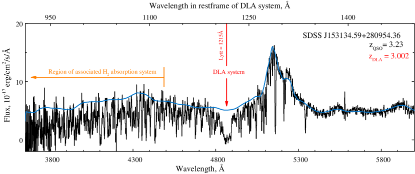
Figure 1: SDSS spectrum of quasar J153134.59+280954.36 ($z_{\rm QSO}=3.23$). The top axis shows the wavelength scale in the restframe of the DLA system which was identified at $z_{\rm DLA}=3.002$. The orange line marks the region of the spectrum where H₂ absorptions (associated with the DLA system) are located. Note, that the signal-to-noise ratio in this region is about 10, which is well above the median S/N of the SDSS spectra. The blue curve shows the estimated quasar unabsorbed continuum.

3 Search of H₂ absorption systems

With such a large number of spectra we need an automatic procedure to search for H₂. For this purpose we used a modification of the standard profile fitting technique which compares an observed quasar spectrum with a synthetic H₂ absorption spectrum.

3.1 Continuum determination

The determination of the quasar continuum is the first important step of any profile fitting routine. We used a combination of two methods: the principal component analysis (PCA) and the iterative smoothing.

The first method reproduces an unabsorbed flux over the Ly$\alpha$ forest by fitting the red part of the spectrum with a combination of principal components (see Pâris et al. 2011). We need to define the continuum in a wider wavelength range ($900\mbox{\AA}<\lambda<1200\mbox{\AA}$ in the restframe of the quasar) compared to what was done by Pâris et al. (2011), they reconstructed continuum between the Ly-$\beta$ and C iv emission lines. To expand the continuum to the region $\lambda<1025$ Å  we used a power law extrapolation of the mean quasar continuum (used in PCA method) adding features which account for the Ly-$\beta$ emission line and the Lyman break cutoff.

In the second method the spectrum is smoothed iteratively. For each iteration we smoothed the spectrum by convolution with a Gaussian function with FWHM about 50 Å. Then pixels deviating from the continuum by more than 3$\sigma$ are excluded at each iteration. The remaining pixels were used in the next iteration. We used four iterations, which was enough for convergence.

We found that the first method tends to overestimate the continuum and sometimes yields an incorrect shape in the presence of sharp features, while the second method tends to underestimate the continuum and to smooth out emission lines. Therefore, the final continuum was constructed as the geometric average of the two continua convolved with a Gaussian function with FWHM$\sim$1000 km/s (an example of reconstructed continuum is shown in Fig. 1). Obviously, the continuum reconstruction in the region bluewards the Ly-$\alpha$ emission line is rather difficult and sometimes ambiguous. Nevertheless, simulations presented in Section 3.3 show that the continuum reconstructed by the described procedure does not introduce any strong bias in the search for H₂ absorption systems. For each spectrum in the samples we determined the signal to noise ratio (S/N) as the mean of S/N in each pixel over the wavelength range 1120$-$1040 Å  in the restframe of the DLA system.

3.2 The searching procedure

Three main difficulties complicate the identification of H₂ absorption systems in SDSS spectra: (i) the intermediate spectral resolution, (ii) the usually low S/N and, (iii) the presence of the Ly-$\alpha$ forest. These difficulties jointly can lead to false identifications of H₂ absorption systems. The SDSS spectral resolution is the most important of them. The pixel size in the blue part of the SDSS spectrum is about 1 Å. It sets a lower limit on the equivalent width of the H₂ lines which can be identified in SDSS spectra. The condition that H₂ equivalent widths to be larger than 1 Å  is fulfilled only for H₂ column density larger than $\log$$N$${\rm{}_{H_{2}}}$ $\gtrsim 18.5$. The molecular hydrogen absorption spectrum in the UV appears as a series of absorption lines corresponding to Lyman and Werner vibrational bands L$\nu$-0 and W$\nu$-0. Intermediate SDSS spectral resolution leaves the possibility to observe only the most prominent lines corresponding to the R(0), R(1) and P(1) transitions in each band. These three absorption lines for each band are overlapped with each other under such resolution. We will refer to these absorption features by the name of the band, i.e. in case L4-0R(0), L4-0R(1) and L4-0P(1) are overlapped, the absorption feature will be denoted as L4-0 absorption line. The typical shapes of these lines are shown in Fig. 2 by blue color.

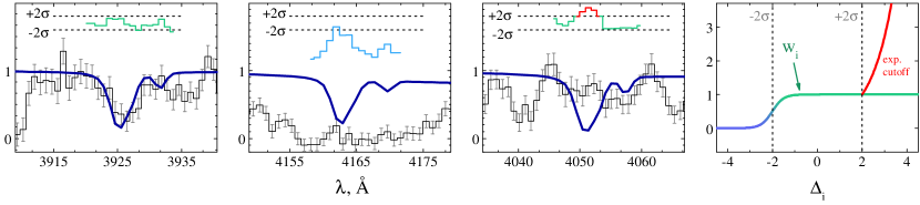
Figure 2: Illustration of the searching criterion. The three left panels show different situations: respectively from left to right, good fit, blended and bad fit. The blue line shows typical profiles of highly saturated (e.g. $\log$$N$${}_{\rm H_{2}}=20$) R(0), R(1) and P(1) lines convolved with the SDSS instrument function. The right panel shows the weight function and exponential cutoff function, that we used in our searching procedure (see equations 1 and 3).

We will construct a template of H₂ absorption systems to fit the SDSS spectra. The H₂ absorption lines (from low rotational levels) have restframe wavelengths $\lambda<1115$ Å. In principle, before the Lyman cutoff (at 912 Å) of the DLA system, 26 absorption lines (from the Lyman and Werner bands) can be observed. However, H i absorption lines of high order Lyman series of the DLA system can substantially absorb the spectrum blueward of $\sim$950 Å. At the SDSS resolution, it leaves only about 17 H₂ lines which can be identified in the spectrum. However, the number accessible H₂ absorption lines varies for different spectra primarily because of the difference between the DLA and quasar redshifts and also because of the spectrum quality (in SDSS spectra S/N usually decreasing with decreasing wavelength). If the quasar redshift is low, the blue end of the spectrum limits the number of fitted H₂ lines. If the quasar redshift is high ($z>2.8$), then the presence of Lyman limit systems or saturated Ly$\alpha$ forest lines at redshift between $z_{\rm QSO}$ and $z_{\rm DLA}$ can reduce the number of H₂ lines in the fit. To characterize the number of fitted lines we determined the cutoff wavelength $\lambda_{\rm cutoff}$ as the position in the spectrum from which the flux exceeds the zero level at the 2$\sigma$ level over more than 4 pixels in a row. In the following we will use the parameter $\lambda_{\rm B}=\lambda_{\rm cutoff}/(1+z_{\rm DLA})$ – the cutoff in the spectrum expressed in the DLA restframe. This parameter just characterizes the number of H₂ absorption lines, that was used in the fit. The pixels corresponding to the DLA Lyman series lines (Ly$\beta$, Ly$\gamma$, etc) were excluded from the fit.

To identify H₂ absorption systems we used the profile fitting technique which compares a real spectrum with a H₂ model spectrum with specified physical parameters (i.e. column density, Doppler parameter, redshift). As we have to search H₂ systems in the large number of spectra ($\sim$ 13 000), we need to develop an automatic procedure. We constructed a function based on the standard $\chi^{2}$ likelihood function commonly used in profile fitting procedures. This function is defined as

$$\log L=\frac{\sum_{i}w_{i}\xi_{i}}{\sum_{i}w_{i}},$$ (1)

where we introduced the weight $w_{i}$ for each pixel

$$w_{i}(\Delta_{i})=\frac{1}{1+e^{-4(\Delta_{i}+2)}},$$ (2)

where $\Delta_{i}=(y_{i}-f(x_{i}))/\sigma_{i}$ is the relative deviation of the model $f_{i}$ from the observed flux $y_{i}$ in pixel $x_{i}$, $\sigma_{i}$ is the error in pixel $x_{i}$. The weight function $w_{i}$ was chosen in the following way (see right panel of Fig. 2). We rejected those pixels (i.e. their $w_{i}=0$) for which the spectrum is more than two $\sigma$ below the model because they are possibly related to blends which are numerous in the Ly-$\alpha$ forest. For pixels where $2>\Delta_{i}>-2$, $w_{i}\approx 1$. The function $\xi_{i}$ is given by

$$\xi_{i}=\left\{\begin{array}[]{l l}\Delta_{i}^{2}e^{(1-\Delta_{i})^{2}-1}&\quad\Delta_{i}\geq 2\\ \Delta_{i}^{2}&\quad\Delta_{i}<2\\ \end{array}\right\},$$ (3)

where for $\Delta_{i}\geq 2$, an exponential cut-off is introduced because in case H₂ is present, all the absorption lines should be consistently seen. Obviously, it is reasonable to fit only the absorbed part of the spectrum. Therefore the sum is taken only over the pixels where the model $f$ is less than 0.9 times the continuum level. Note, that the introduction of the exponential factors implies that $L$ defined by Eq. (1) is not a likelihood function. The function $L$ is used only to select H₂ system candidates. We will estimate the confidence level of the detection in Sect. 4. We set the criterion of identification as $L<L_{id}$, where $L_{id}$ is the value of $L$ with $\Delta_{i}=2$ for all pixels ($w_{i}\approx 1$ when $\Delta_{i}=2$) at certain redshift. This criterion is fulfilled in case of the satisfactory fit of spectrum by H₂ absorption system model, i.e. there are no outliers in pixels, where observed flux is sufficiently larger than fit flux.

In standard profile fitting the best fit is obtained by minimization of a likelihood function over the parameter space. However, such a process requires to calculate a large number of absorption profiles which in our case would be particularly computational demanding. Rather we constructed a set of H₂ absorption system template spectra on a dense grid of total column density and effective excitation temperature. These two parameters mainly define the line profiles of saturated H₂ absorptions at a given spectral resolution. The total H₂ column density ranges from log $N$(H₂) = 18.5 to 21 by step of 0.1 dex. With column densities less than 18.5 the absorption lines become weak and reliable identification of H₂ is impossible (see Sect. 4.2). The effective excitation temperature, $T_{\rm 01}$, specifies the relative populations of H₂ J=0 and J=1 levels. $T_{\rm 01}$ was varied from 25 to 150 K corresponding to the typical observed range (Srianand et al., 2005). The Doppler parameter is not important since we considered only highly saturated absorption systems ($\log{N}>18.5$). An important ingredient is the velocity structure of the absorption system, i.e. the number of components, their relative strengths, and positions. High resolution observations show that more than 50 per cent of the H₂ absorption systems are multicomponent. However, the typical velocity separation of these components is less than 50 km/s which is smaller than the SDSS spectral resolution ($\sim 150$ km/s). Therefore, we use a single component model. This implies however that our inferred H₂ column densities can be overestimated. This is partially confirmed by the analysis of the H₂ systems previously identified in high resolution spectra (see Sect. 5).

We have implemented a fully automatic searching procedure. For each spectrum in the S_DLA sample we calculated $L$ function in the redshift window for each model of H₂ absorption system in the template. The redshift window was taken as $\pm$600 km/s around the redshift of the DLA system. The DLA redshifts were taken from Noterdaeme et al. (2009, 2012). Note that the value 600 km/s is larger than the typical observed velocity dispersion for H₂ absorption systems in DLAs. For each H₂ absorption system model from the template we have searched for redshifts at which identification criterion $L<L_{id}$ is satisfied. Note that function $L$ guarantees that if H₂ absorption system with column density $N_{0}$ is satisfied $L<L_{id}$ for some position $z$ then H₂ absorption system with column density $N<N_{0}$ (less saturated) will also satisfied $L<L_{id}$ at $z$.

Applying our searching procedure to the S_DLA sample we have selected a preliminary S_cand sample of H₂ system candidates. For each candidate in the sample we have recorded the largest total column density for which $L<L_{id}$ is satisfied and the value of $z_{0}$ where $L$ has minimum for this largest total column density. The preliminary sample of candidates, S_cand, contains over 4 000 records. However most of these candidates are false detections caused mainly by Ly-$\alpha$ forest features in low S/N spectra. Indeed the observed occurrence rate of H₂ candidate in DLA based on the preliminary sample ($\sim$4000/13000=0.3) is larger than the $<$0.1 estimated rate based on high resolution data (Noterdaeme et al., 2008a). To select most promising candidates for follow-up spectroscopic studies we need to select only candidates with high confidence, i.e. the candidates with a low probability of false detection. Two methods to estimate the probability of false detection are described in Sect. 4.

3.3 Testing the searching procedure

We need to be convinced that the overwhelming majority of real H₂ absorption systems will be detected by the searching procedure. One of necessary conditions is that the known H₂ absorption systems should be detected by our procedure in SDSS data. There are only five such systems with SDSS data. They are listed in Table 2 and will be discussed in Section 5. Only three of these spectra are useful because of the proper spectral wavelength range. The searching procedure detects H₂ in all of them. This is fine but not enough to be convinced of the robustness of the searching procedure. Therefore we have tested the searching procedure on the data where we artificially added H₂ systems. For this we have used the S_nonDLA sample (where there are no DLA systems, see Sect. 2) and artificially added DLA systems with one H₂ component with a specified column density $N$ at a given redshift. We used each spectrum several times varying the DLA redshift to increase statistics. With this procedure we are sure that we have the same situation of noise and redshift distribution as in our search sample.

After applying our searching procedure we find that the typical non-detection rate (i.e. the fraction of systems we miss) is less than 1%. The dependence of the non-detection rate with the specified column density is shown in Fig. 3.

We conclude that our searching procedure gives a sample which is complete at the $>99\%$ level for log $N$(H₂) $>$ 18. However, as we will show in the following section at such column densities the false identifications dominate the candidate sample and the limit column density for reliable identification is log $N$(H₂) $>$ 19. For column density log $N$(H₂) $>$ 19 our searching procedure gives completeness at more than $99\%$ level.

Figure 3: Non-detection rate of the searching procedure versus log $N$(H₂). This rate is found to be less than 1%.

4 Confidence estimation

In the previous Section we have shown that our procedure is able to identify strong H₂ absorption systems in SDSS spectra when they are present. However, at this resolution, the numerous Ly-${\alpha}$ forest lines can easily mimic an H₂ absorption system and lead to false identifications. Therefore, in order to select a robust sample of H₂ system candidates, we need to estimate the confidence level of the candidates, i.e. the probability for an H₂ candidate to be real. For this we determined a false identification probability (FIP). It is the probability to wrongly select an H₂ absorption system in some realization of the Ly-$\alpha$ forest. If FIP is small, then the selected H₂ absorption system is likely to be real, i.e. its confidence value is high.

We have applied two methods for FIP determination. In the first method for each possible detection, we have calculated the probability that a similar absorption system is detected anywhere else in the spectrum (see Sect. 4.1). In the second method we have calculated the rate of H₂ absorption system identification in the samples of spectra where there are confidently no H₂ absorption systems, i.e. in control samples. The latter method presented in Sect. 4.2 allows us in addition to estimate a detection threshold of H₂ absorption system in SDSS spectra and the detection probability of H₂ absorption systems in DLAs.

4.1 Monte-Carlo sampling

The main point of this method is H₂ absorptions to be numerous, so as a typical system will be detected by about 6-15 absorption features. Suppose that the probability to “fit” by chance one H₂ line in the forest is 0.5. This means that the absorption line satisfies the identification criterion ($L<L_{id}$) over half of any wavelength window. Then the chance to “fit” $N$ lines together would be about $(0.5)^{N}$. The joint probability to fit a H₂ system by chance in a forest where no H₂ system is present can thus be very small. Therefore it is reasonable to expect that we can identify H₂ absorption systems even at the SDSS resolution and spectral quality.

To estimate the confidence of each candidate in the S_cand sample we used the following procedure. We performed arbitrary random shifts of the H₂ absorption lines detected in the candidate. The shift of each line was limited by the position of the adjacent H₂ lines in the spectrum, typically less than 4000 km/s. In other words, we randomly “shake” the H₂ absorption line positions. We performed many realizations and for each one we calculated the value of the $L$ criterion. The identification probability is estimated as:

$$f_{\rm FP}=n(L<L_{id})/n_{\rm all},$$

where $n(L<L_{id})$ is the number of identifications, i.e. realizations that satisfied ($L<L_{id}$), and $n_{\rm all}$ is the total number of realizations. The value of $f_{\rm FP}$ can be simply described as the probability of joint fit of several absorption lines in the particular realization of the Ly-$\alpha$ forest in the spectrum. If $L<L_{id}$ for the majority of realizations, then $n(L<L_{id})$ is close to $n_{\rm all}$ and $f_{\rm FP}$ is close to 1. In this case Ly-$\alpha$ forest can effectively mimic the absorption system and the identification cannot be considered as robust. If $L<L_{id}$ in a few of many realizations, then $f_{\rm FP}$ approaches 0. In this case the probability of the Ly-$\alpha$ forest to mimic the absorption system is small and the confidence in the identification of the system is high. It should be emphasize that this method takes naturally into account the peculiarities of each spectrum.

The value of $f_{\rm FP}$ gives an estimate of the FIP for the candidate. However H₂ absorption lines have rigid relative position, while in the above calculation of $f_{\rm FP}$ we used random relative positions to increase statistics. We note that applying random shifts to H₂ absorption lines with respect to a fixed Ly-$\alpha$ forest is equivalent to applying random shifts to Ly-$\alpha$ forest lines with respect to fixed H₂ absorption. The latter would be difficult to realize technically, therefore we shifted H₂ absorption lines from their positions. Nevertheless it is necessary to estimate the $f_{\rm FP}$ value at which the detection can be considered as robust. To do this we used the following steps. We have applied the searching procedure to the SDSS spectra without DLA systems. We chose subsample, S${}^{\prime}_{\rm nonDLA}$, of the control sample S_nonDLA with size equal to the size of S_DLA sample. For each spectrum with z_QSO from the S${}^{\prime}_{\rm nonDLA}$ subsample we have generated the redshift of a “fictitious” DLA system using the distribution of z_DLA in the subsample of S_DLA spectra which have QSO redshifts in the range z${}_{\rm QSO}\pm 0.1$. The absence of real DLA systems in the spectra of S${}^{\prime}_{\rm nonDLA}$ subsample guarantees that there is no H₂ absorption system in the spectrum. We searched for “H₂ candidates” in this sample which are almost certainly false identifications. For each of the selected “H₂ candidate” we have calculated $f_{\rm FP}$. The distributions of $f_{\rm FP}$ values for the S_DLA (indicated as discrete measurements) and S${}^{\prime}_{\rm nonDLA}$ (smooth profiles) samples are shown in Fig. 4 versus the H₂ column densities. It is apparent that a value of $\log f_{\rm FP}<-3$ can be considered as the limit for reliable identification, as there is sufficient excess in the distribution of the candidates from the S_DLA sample.

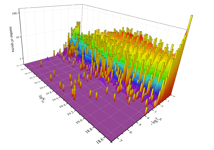
Figure 4: The distributions of $f_{FP}$ values versus the column density of the H₂ absorption system candidates. The orange columns show the calculated distribution using the S_DLA sample (where H₂ systems are to be found), while smooth profiles show the distribution calculated from the S_nonDLA control sample (where no H₂ systems are expected). The value of $\log(f_{\rm FP})=-3$ can be considered as the threshold for robust identification, since there are only a few spectra from the S_nonDLA control sample with smaller $f_{\rm FP}$ values.

4.2 Use of a control sample

The FIP of an H₂ absorption system can be estimated as the rate of identifications in spectra where no H₂ absorption system is expected.

FIP mainly depends on the quality of the spectrum, density of the Ly-$\alpha$ forest and certain profile of H₂ absorption system. We took four parameters (which we found enough) to describe this dependence: $z_{\rm QSO}$, S/N, $N_{\rm H_{2}}$ and the number of H₂ absorption lines that can be seen in the spectrum. We characterize the latter by the parameter $\lambda_{\rm B}=\lambda_{\rm cutoff}/(1+z_{\rm DLA})$ which is the blue limit of the spectrum expressed in the DLA restframe. H₂ absorption lines have rest-wavelength $\lambda<$1110Å . In order to detect at least one H₂ line, $\lambda_{B}$ must be $<$ 1110 Å. FIP has to be determined at each combination of these parameters. We have calculated FIP on a grid of H₂ column densities, S/N, $\lambda_{\rm B}$ and z_QSO parameters values. Log(S/N) was considered from 0.2 to 1.4 by step of 0.1. The different values of $\lambda_{\rm B}$ were taken to correspond to an increment in the number of H₂ lines. The redshift of QSO, $z_{\rm QSO}$, was varied in the range from 2.2 to 4.2 with 0.4 step.

For each spectrum in the S_nonDLA control sample we chose randomly several positions of $z_{\rm DLA}$. Each of z_DLA for the spectrum corresponds to different number of H₂ absorption lines involved in analysis, or $\lambda_{\rm B}$ bin. Therefore one spectrum can be used several times with different z_DLA. In other words, we constructed enlarged sample S${}^{\prime}_{\rm nonDLA}$, which allowed us to sufficiently increase statistics. Then we have applied the searching procedure (see Sect 3.2) to enlarged sample S${}^{\prime}_{\rm nonDLA}$ and have calculated the identification rate for each H₂ column density in the selected S/N and $\lambda_{\rm B}$ bins

$$f_{\rm CS}(\lambda_{\rm B},S/N,{\rm z_{QSO}},N_{\rm H_{2}})=n(L<L_{id})/n_{\rm bin},$$ (4)

$n(L<L_{id})$ is the number of spectra in the bin, for which the identification criterion ($L<L_{id}$) is satisfied, $n_{\rm bin}$ is the total number of spectra in the bin. The identification rate in the S_nonDLA sample gives us the estimate of the FIP. The contour plots of $f_{\rm CS}$ for different $N_{\rm H_{2}}$ are shown on Fig. 5. $f_{\rm CS}$ depends mainly on $\lambda_{\rm B}$ and S/N and little on $z_{\rm QSO}$. Therefore to construct the contour plots we integrated $f_{\rm CS}$ over the $z_{\rm QSO}$ bins. The dependence of FIP, $f_{\rm CS}$, on $z_{\rm QSO}$ is shown in Fig. 6. Note that the contour plots shown on Figs. 5 and 6 are smoothed over the bins. The general behavior of $f_{\rm CS}$ satisfies reasonable expectations. The probability decreases with decreasing $\lambda_{B}$ (i.e. increase of the number of available H₂ lines), and with increasing S/N and decreasing $z_{\rm QSO}$ (forest less dense). Additionally, the probability decreases with increasing total H₂ column density N${}_{\rm H_{2}}$.

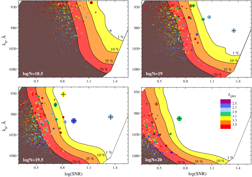
Figure 5: Contour plots of false identification probability of H₂ absorption systems estimated by using the control sample S${}^{\prime}_{\rm nonDLA}$. The different panels show $f_{\rm CS}$ for different $\log N$ - the total H₂ column density. Y-axis correspond to $\lambda_{\rm B}$ - a parameter characterizing the number of H₂ bands available. X-axis corresponds to the signal-to-noise ratio of the spectrum. The white, yellow, orange, red and brown regions correspond to FIP values $<$1%, $<$10%, $<$35% and $<$70%, respectively. The black crosses show our candidates H₂ absorption systems. The size of each cross corresponds to the value of $f_{\rm FP}$ estimated from the Monte-Carlo method. The bigger size, the lower $f_{\rm FP}$ value. The color of each cross corresponds to the redshift of the candidates.

The calculated identification rate $f_{\rm CS}$ gives an upper limit on the FIP of H₂ absorption system. Indeed, we searched H₂ system in some redshift window around z_DLA. The probability that at some redshift in the search window identification criterion to be satisfied increase with increase of search window width. Therefore the rate $f_{\rm CS}$ is scaled with changing the search window width. The rate $f_{\rm CS}$ approaches FIP value with reducing search window width. However, we can’t set search window very small since we do not know the exact position of H₂ system relative to z_DLA (which sets the center of the search window).

To estimate the false identification probability of our H₂ candidates derived from the S_cand sample we have to position the corresponding spectra on Fig. 5. The candidates can be seen as crosses. The size of each cross indicates the calculated false identification probability from the Monte-Carlo method (see sect. 4.1). Note that the FIP estimated from the two methods are in agreement. It is apparent that the overwhelming majority of candidates are located in regions where the FIP probability is high, i.e. these identifications are not robust. However, some spectra are located in regions with low false identification probability.

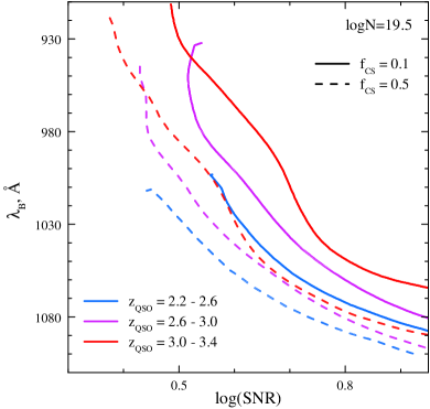
Figure 6: Dependence of the $f_{\rm CS}$ (the upper limit on the false identification probability) on $z_{\rm QSO}$. Solid and dashed lines show the $f_{\rm CS}$ isocontours at $0.1$ and $0.5$, respectively. The $f_{\rm CS}$ is calculated for log $N$(H₂)(cm^-2) = 19.5. Blue, purple and red lines correspond to $f_{\rm CS}$ calculated using spectra with $z_{\rm QSO}$ in the ranges ($2.2\div 2.6$), ($2.6\div 3.0$) and ($3.0\div 3.4$), respectively.

Using these considerations, we can estimate the thresholds in S/N and $\lambda_{B}$ for robust identification at a given $N_{\rm H_{2}}$ at some $f_{\rm CS}$ level. We note that the detection limit of H₂ absorption systems in SDSS spectra is higher than $\log$N$\sim 19$. Indeed, it is seen from Fig. 5 that for confident detection, $f_{\rm CS}<10\%$, of H₂ absorption system with column density $\log$N$\sim 19$ the high signal to noise spectrum is required. Such spectra are very rare in SDSS database.

Sample S${}^{\prime}_{\rm nonDLA}$ has a limited number of spectra in some bins of the parameter space, especially at high S/N and low $\lambda_{B}$ value. Additionally we have used each spectrum several times. Therefore, we used simulated spectra to check the influence of these limiting factors. We generated a S_Lyα sample quasar spectra. The overall shape of the continuum was constructed using principal component coefficients from Pâris et al. (2011) (we used only the 10 first PCA coefficients). The Ly$\alpha$ forest column density and Doppler parameter distributions and the evolution with redshift of the number density were taken from Meiksin (2009). The initial spectrum was calculated at high resolution ($>$ 100,000) and then convolved with the SDSS BOSS instrumental function taken from Smee et al. (2013). Finally, we added Poisson noise corresponding to the SDSS sample. We generated a substantial number of spectra ($\sim$ 400) in each bin of $\lambda_{B}$ and S/N. We applied our searching procedure and calculated the identification rate in each bin. We find that $f_{\rm CS}$ estimated from the SDSS DR9 sample and from the mock sample generally are agree within statistical errors.

4.3 Probability of H₂ detection in DLAs

The FIP estimated in the previous section allows us to determine the probability of H₂ detection in DLA systems. For each column density we have selected the regions of the $\lambda_{B}$-S/N parameter space (shown on Fig. 5) where $f_{\rm CS}$ is less than a given threshold value. In principle it is better to use as low threshold value as possible, because this reduces possible biases and increases the robustness of the detection. However, in order to increase statistics, we have taken a threshold value of $50\%$. We checked that lower threshold values give consistent results, with larger statistical errors. In each bin of the $\lambda_{B}$-S/N parameter space we compared the identification rates of H₂ absorption systems in the S_DLA and S${}^{\prime}_{\rm nonDLA}$ samples. The probability of detection of H₂ systems with column density larger than a given value $N_{\rm H_{2}}$ can be calculated as

$$P({\rm N_{H_{2}}})=\frac{\sum{N_{S_{\rm DLA}}\times(f_{\rm CS}(S_{\rm DLA})-f_{\rm CS}(S^{\prime}_{\rm nonDLA}))}}{\sum{N_{S_{\rm DLA}}}},$$ (5)

where sums are taken over the bins with $f_{\rm CS}(S^{\prime}_{\rm nonDLA})$ less than some threshold value, and $N_{S_{\rm DLA}}$ is the number of spectra with DLA systems in the bin, $f_{\rm CS}(S_{\rm DLA})$ and $f_{\rm CS}(S^{\prime}_{\rm nonDLA})$ are the detection rates of H₂ absorption systems in the bin in the $S_{\rm DLA}$ and $S^{\prime}_{\rm nonDLA}$ samples, respectively. The results of the calculation for two threshold values are shown in Fig. 7. The higher threshold values give larger statistics and therefore smaller error bars. However, calculation using higher threshold values lead to higher values for obtained probability, which is seen in Fig. 7. Nevertheless, the results of the calculation for threshold values 0.1 and 0.5 are in the agreement with each other. Note that this probability, especially at the low column densities, should be considered as an upper limit because our procedure tends to overestimate the column density due to the quality of SDSS spectra.

Based on the VLT survey of H₂ absorption systems in QSO spectra (Noterdaeme et al., 2008a) it was found that the overall covering factor of H₂ in DLAs is $\sim$10% for $\log f>-4.5$. For the high end of the N(H₂) as considered here, the VLT survey indicates rather 8% (N(H₂)$>$18) or less, in very good agreement with our analysis.

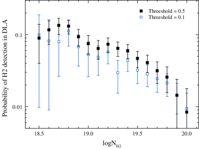
Figure 7: Detection probability of H₂ absorption systems in DLAs versus column density. Note that this probability should be considered as an upper limit because our H₂ column densities are generally overestimated. Blue open and black filled squares correspond to the calculation with 0.1 and 0.5 threshold values of the detection rate, respectively.

5 Candidates

We have compiled the final sample, S_final, of the most promising H₂ candidates for follow up studies. Fig. 8 shows the $f_{\rm FP}$ and $f_{\rm CS}$ values calculated for each candidate in the S_cand sample by the two methods presented in Sect. 4.1 and  4.2, respectively. As we stated above $f_{\rm CS}$ calculated using the control sample gives an upper limit on the FIP, as it depends on the width of the search window. In turn $f_{\rm FP}$ estimated using Monte-Carlo simulations gives a lower limit on FIP. Nevertheless it is seen again that Monte-Carlo sampling and control sample methods are in agreement with each other. The S_final sample presented in Table 1 is formed from new H₂ candidates which have $\log f_{\rm FP}<-3$ (see Fig. 4) and $f_{\rm CS}<0.1$. The selected candidates are shown in Fig. 8 by red circles. The known H₂ absorption systems shown in Fig. 8 by blue points were excluded from the S_final sample and not listed in Table 1. The filled and open circles in Fig. 8 correspond to candidates from DR9 and DR7, respectively. We found that improved quality of quasar spectra in SDSS-III has major importance for detection of H₂ absorption systems. There are only two candidates (J081240.69+320808.52, J153134.59$+$280954.36) in DR7 satisfied the selection criterion for S_final sample ($\log f_{\rm FP}<-3$ and $f_{\rm CS}<0.1$). They were both reobserved and presented DR9 catalog thus we used its DR9 spectra.

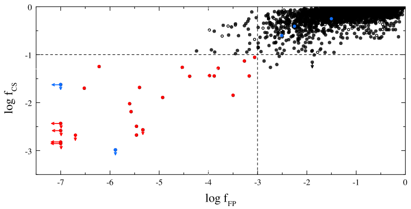
Figure 8: The outputs of the two methods used to estimate the confidence level of H₂ candidates are used to select the final sample. Red circles show selected H₂ candidates. Filled and open circles correspond to candidates from DR9 and DR7, respectively. Blue circles show the known H₂ absorption systems. Two of them (J081240.69+320808.52 and J123714.61+064759.64) are easily found by our method.

Quasar	Plate-MJD-Fiber	$z_{em}$	$z_{DLA}$	$\log$N${}_{\rm H\,I}$	S/N	$\lambda_{B}$, Å	$\log$N${}_{\rm H_{2}}$	T01	$log(f_{\rm FP})$	$f_{\rm CS}$	$\Delta_{V}$
J234730.76$-$005131.68	4214-55451-0212	2.63	2.5874	20.20	0.9	996	19.5	25	$<$-7.0	0.1	-60
J221122.52$+$133451.24	5041-55749-0374	3.07	2.8376	21.85	0.7	993	20.1	25	$<$-7.0	$<$ 0.1	-70
J114824.26$+$392526.40	4654-55659-0094	2.98	2.8320	20.84	1.0	960	19.4	25	$<$-7.0	$<$ 0.3	-30
J075901.28$+$284703.48	4453-55535-0850	2.85	2.8221	20.87	1.1	955	19.2	25	$<$-7.0	$<$ 0.4	-70
J153134.59$+$280954.36	3959-55679-0862	3.23	3.0025	21.01	0.8	932	19.5	25	-6.7	$<$ 0.2	60
J001930.55$-$013708.40	4366-55536-0874	2.53	2.5284	20.64	0.5	1032	20.7	25	-6.5	2.0	-130
J152104.92$+$012003.12	4011-55635-0218	3.31	3.1410	21.56	0.5	958	20.2	25	-6.2	5.6	-150
J013644.02$+$044039.00	4274-55508-0691	2.81	2.7787	20.47	0.7	979	19.7	25	-5.6	1.0	-110
J105934.34$+$363000.00	4626-55647-0381	3.77	3.6402	20.97	0.8	955	19.3	25	-5.6	0.7	-80
J164805.16$+$224200.00	4182-55446-0880	3.08	2.9900	21.52	0.7	957	19.6	25	-5.5	0.3	-40
J160638.54$+$333432.89	4965-55721-0091	3.09	3.0845	20.42	0.9	927	19.2	25	-5.5	0.2	-80∗
J123602.11$+$001024.60	3848-55647-0266	3.03	3.0289	20.58	0.5	938	19.9	25	-5.4	2.1	-4201
J144132.27$-$014429.40	4026-55325-0848	2.98	2.8908	21.46	0.7	959	19.7	25	-5.3	$<$ 0.3	110∗
J150739.67$-$010911.16	4017-55329-0647	3.10	2.9743	20.05	0.6	958	19.8	25	-4.9	1.3	-30
J150227.22$+$303452.68	3875-55364-0040	3.33	3.2828	20.83	0.9	927	19.0	25	-4.5	5.5	0
J082102.66$+$361849.68	3760-55268-0364	2.81	2.8030	20.38	0.6	994	19.7	25	-4.4	3.5	-10
J084312.72$+$022117.28	3810-55531-0727	2.91	2.7866	21.80	0.4	1040	21.0	25	-4.0	3.6	-10
J123052.64$+$020834.80	4752-55653-0116	3.36	2.7981	21.26	0.8	1015	19.7	25	-3.9	3.6	20
J082716.26$+$395742.48	3761-55272-0810	2.83	2.7420	20.59	1.0	956	18.8	25	-3.8	5.2	50
J004349.39$-$025401.80	4370-55534-0422	2.96	2.4721	20.57	0.6	1029	20.1	25	-3.5	1.4	2702
J120847.64$+$004321.72	3845-55323-0604	2.72	2.6083	20.35	1.0	993	18.8	25	-3.3	7.4	-40
J160332.00$+$081622.44	4893-55709-0876	2.86	2.8429	20.27	0.9	942	18.9	25	-3.2	3.6	-10
J141205.80$-$010152.68	4035-55383-0704	3.75	3.2678	20.53	0.9	1007	19.1	25	-3.1	8.8	30

Table 1: The S_final sample of new H₂ absorption system candidates in SDSS DR9. Here $z_{em}$, $z_{DLA}$ and $\log$N${}_{\rm H\,I}$ (cm^-2) are quasar and DLA system redshifts and column density of H i taken from Noterdaeme et al. (2009), S/N is $\log$ of estimated signal to noise ratio of the spectrum in the region where H₂ lines should be seen, $\lambda_{B}$ is wavelength of the cutoff in the spectrum in the DLA restframe, $\log$N${}_{\rm H_{2}}$ (cm^-2) is estimated upper limit on the H₂ total column density, $T_{01},{\rm(K)}$ is kinetic temperature which gives the relative population of J=0, J=1 H₂ rotational levels, $f_{\rm FP}$ is the probability of false detection estimated by Monte-Carlo sampling, see Sect. 4.1, $f_{\rm CS}$ is the probability of false detection estimated by control sample expressed in per cent, see Sect. 4.2, $\Delta_{V}$, km/s is the difference between redshifts of H₂ bearing component and DLA system (measured by metal lines). ^∗ C i metal lines are tentatively detected in these spectra. It is believed that C i is a good tracer of H₂. ¹ in this DLA system H₂ bearing component associated with the second, less prominent component in metal line profile. ² low ionization metal lines is not detected in this system. z_DLA estimated using C iv and Si iv metal transitions. Visual inspection showed that this candidate is unlikely.

Note, that the H₂ column densities given in Table 1 are generally overestimated. This arises mainly from two factors. The first is the numerous blends in the Ly$\alpha$ forest which can be unresolved at the resolution of SDSS spectra. The second is that our procedure gives the highest column density for which the criterion of detection, $L<L_{id}$, is satisfied. We found that SDSS data quality is not high enough to estimate with reasonable uncertainty H₂ column densities using standard $\chi^{2}$ likelihood profile fitting. Using simulations of SDSS mock spectra with specified H₂ absorption systems we can estimate that the standard $\chi^{2}$ procedure gives systematic errors larger than 0.5 dex.

High resolution spectrum studies of H₂ absorption systems ($\log$ N $\gtrsim 19$) indicate that H₂ bearing DLA systems usually are associated with prominent metal lines. We found that the redshifts of H₂ bearing component of the candidates is satisfied with redshifts of DLA system within 100 km/s, which is less than errors in the redshift determinations. Only in two of the H₂ candidates (see Table 1, they marked by an asterisk) we have detected C i absorption lines which is known as a good tracer of molecules (Srianand et al., 2005; Noterdaeme et al., 2012). Detections of C i are rare in SDSS spectra as a consequence of the low resolution of the spectra.

For instance, we present two candidates in the spectra of J234730.76-005131.68 and J084312.72+022117.28 in Fig. 9 and Fig. 10, respectively. The J234730.76-005131.68 spectrum has relatively high S/N and the candidate has very low $f_{\rm FP}$ value, i.e. the detection of the H₂ absorption system is robust. The J084312.72+022117.28 spectrum has lower S/N and the candidate higher $f_{\rm FP}$ value, but from Fig. 10 it can be seen that highly saturated H₂ absorptions are prominent. The estimated column density of this H₂ candidate is $10^{21.1}$ cm^-2. Such high H₂ column densities have never been observed towards high redshift quasars. There are also 3 candidates in Table 1, which have estimated column densities exceeding $10^{20}$ cm^-2. Such saturated H₂ systems are detected up to now only towards two GRBs (Prochaska & Wolfe, 2009; Krühler et al., 2013), and are usual in our Galaxy (Rachford et al., 2002). These four selected highly saturated H₂ systems are very promising candidates to probe the translucent phase of high redshift ISM.

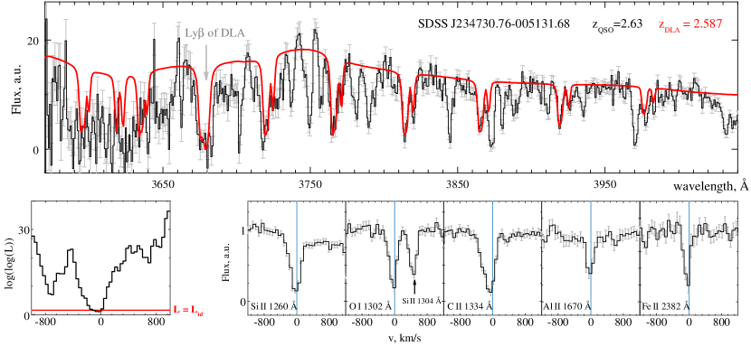
Figure 9: The spectrum of SDSS J234730.76-005131.68. The top panel shows part of the spectrum with fitted H₂ profiles at z=2.587 overplotted. The five right bottom panels show metal lines associated with this system. Left bottom panel shows the dependence of the searching criterion with redshift, expressed as a velocity offset from the position of the system.

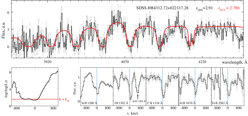
Figure 10: The candidate in the spectrum of SDSS J084312.72+022117.28 has possibly the highest column density ever detected in front of QSOs, $\log N_{\rm H_{2}}=21.1$. The top panel shows part of the spectrum with fitted H₂ profiles. The five right bottom panels show metal lines associated with this system. Left bottom panel shows the dependence of the searching criterion with redshift, expressed as a velocity offset from the position of the system.

Table 2 gives the properties of seven H₂ absorption systems that were previously identified from high resolution spectra obtained at Keck and/or VLT observatories. One of them (J143912.04+111740.5) was not included in the DLA catalog due to poor S/N, but we included the spectrum in the searching sample, S_DLA. For two of them H₂ lines fall out the searched region due to poor spectral quality. We identify the H₂ absorption systems in all of the five remaining spectra. However the identification is robust only for two systems. They have $\log$N_HR(H₂) $>$ 19 measured from high resolution data. For the other three systems (J144331.17+272436.73, J081634.39+144612.36, J235057.87-005209.84) with H₂ column density $\log$N_HR(H₂) lower than 19, our false identification probability is not low enough $>10^{-3}$, i.e. identification is not robust and they can not be considered as reliable candidates.

Quasar	$z_{em}$	$z_{abs}$	$\log$(S/N)	$log(f_{\rm FP})$	$\log$ N	$\log$ NHR	Instrument	comment	ref.
J081240.69+320808.52	2.70	2.625	1.4	$<$-7.0	19.8	19.88$\pm$0.06	KECK/HIRES	HD	a
J123714.61+064759.64	2.79	2.689	0.8	-5.5	19.9	19.21${}^{+0.13}_{-0.12}$	VLT/UVES	multicomp, HD/CO	b
J144331.17+272436.73	4.44	4.225	0.6	-2.5	19.2	18.29$\pm$0.08	VLT/UVES		c
J081634.39+144612.36	3.85	3.287	0.6	-1.7	19.8	18.66${}^{+0.17}_{-0.30}$	VLT/UVES	multicomp	d
J235057.87-005209.84	3.02	2.425	0.6	-1.4	19.7	18.52${}^{+0.30}_{-0.49}$	VLT/UVES	multicomp	e
J143912.04+111740.5	2.58	2.418	0.6	Out of range		19.38$\pm 0.10$	VLT/UVES	multicomp, HD/CO	f
J091826.16+163609.0	3.07	2.58	0.1	Out of range		19$\div$16	VLT/X-shooter	not in DLA sample	g

Table 2: Already known H₂ system in SDSS. $log(f_{\rm FP})$ is a estimate of FIP, estimated by Monte-Carlo sampling method. $\log$ N is the H₂ column density estimated by our procedure. $\log$ N_HR is H₂ column density known from analysis of high resolution spectrum. Ref.: ^a Jorgenson et al. (2009), ^b Noterdaeme et al. (2010), ^c Ledoux et al. (2006), ^d Guimarães et al. (2012), ^e Petitjean et al. (2006), ^f Srianand et al. (2008), ^g Fynbo et al. (2011).

6 Properties of H₂ candidate sample

In this Section we present the properties of candidates in the S_final sample. The main goal is to search for difference between the properties of H₂-bearing and non H₂-bearing DLA systems. The distributions of neutral hydrogen column density for H₂ candidate sample and DLA sample are shown in Fig. 11. The Kolmogorov-Smirnov test indicates that we can reject the hypothesis that the two distributions are the same at the 0.99 level. Comparison of the distributions shows that the presence of high column density H₂ absorption systems lead to the higher H i column densities.

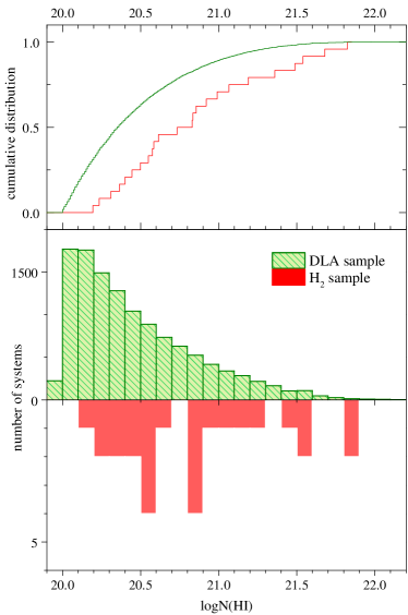
Figure 11: Distribution (bottom panel) and cumulative distribution (top panel) of the column densities of neutral hydrogen in the DLA systems. Red and green colors correspond to the sample of H₂ bearing candidates and S_DLA sample, respectively.

6.1 Colour excess

We have studied the colour excess for the H₂ candidate sample, S_final. Recently it was shown that quasar spectra with H₂/CO-bearing absorption systems show significant $g-r$ colour excess compared to quasar spectra with non-molecular bearing DLAs (e.g. Noterdaeme et al. 2010). This excess might be caused by: (i) the presence of H₂ absorption lines in H₂ candidate spectra; (ii) the increased dust content of the H₂ bearing DLA (because H₂ molecules in the cold neutral medium mainly form onto the dust grains). To estimate the colour excess we used the following procedure. SDSS filters magnitudes were taken from the DR9 quasar catalog (Pâris et al., 2012). For each H₂ candidate we have selected a control sample of quasars from the DR9 catalog with redshifts similar to redshift of the candidate quasar (within $\Delta z=0.05$). We have compared the value of $r-i$ color for each candidate with the median value of $r-i$ in the control samples (the top right and left panels of Fig. 12). In comparison with previous studies we have chosen $r$ and $i$ filters because there is no bias due to the presence of H₂ absorption lines. Using dispersions measured in the control samples we have calculated standard deviations of the candidates from their control samples (the middle right panel of Fig. 12). We have found 1$\sigma$ excess in the $r-i$ colors for H₂ candidate sample from their control samples. Additionally, we have found that $r-i$ color excesses for H₂ candidates are statistically higher than color excesses measured for the DLA sample (for this purpose we used the statistical DLA sample from Noterdaeme et al. (2012), which is a subsample of S_DLA sample), see Fig. 13. Since H₂ absorption lines for H₂ candidate do not fall in $r$ and $i$ SDSS filters we suppose that this excess is the evidence of enhanced dust content in H₂-bearing DLAs. We found significant excesses of H₂ candidate sample over DLA sample in $g-r$, $u-r$, $r-z$ colours as well. The excesses in $g-r$, $u-r$ colors are about 2$\sigma$ of standard deviation, that are higher than $\sim 1\sigma$ excesses measured in $r-i$, $r-z$ (see Fig. 14). It agrees with previous statement about higher extinction in H₂ bearing candidates, but can be also explained by location of H₂ absorption lines over $g$ and $u$ SDSS filters. The Fig. 14 shows comparison of standard deviations from their control samples of H₂ candidate and DLA samples, calculated for $g-r$ and $r-z$ colors. We suppose that measured colour excesses most likely are explained by the higher amount of dust in the H₂-bearing DLAs. The latter can be investigated further by extinction measurement from spectral fitting.

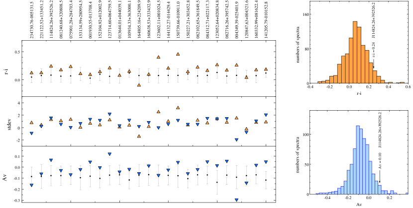
Figure 12: Estimated $r-i$ colors and $A_{V}$ for selected H₂ candidates. Top left: the orange points in the top left panel show the $r-i$ color for H₂ candidates while the black points with error bars show the median value and dispersion of $r-i$ colors in control samples for each of the H₂ candidates. Bottom left: the blue points in the top left panel show the $A_{V}$ for H₂ candidates while the black points with error bars show the median value and dispersion of $A_{V}$ in control samples for each of the H₂ candidates. Middle left: orange and blue points indicate standard deviation of $r-i$ and $A_{V}$, respectively, measured for H₂ candidates from their control sample. Top right: distribution of $r-i$ colour in the control sample of H₂ candidate in J114824.26+392526.2. Bottom right: distribution of $A_{V}$ in the control sample of H₂ candidate in J114824.26+392526.2.

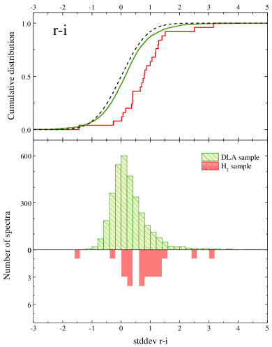
Figure 13: Distribution (bottom panel) and cumulative distribution (top panel) of the standard deviations of $r-i$ compared to the median in the control samples. Red and green colors correspond to the sample of H₂ bearing candidates and DLA sample, respectively. The black dashed line in the top panel shows the cumulative probability for a normal distribution.

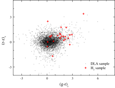
Figure 14: $(r-z)_{r}$ – $(g-r)_{r}$ color diagram. Red and black points correspond spectra from the sample of H₂ bearing candidates and DLA sample, respectively. $(r-z)_{r}$ and $(g-r)_{r}$ values show $r-z$ and $g-r$ colors measured in standard deviations of their control samples.

6.2 Extinction

The 1$\sigma$ $r-i$ colour excess of H₂ candidates can indicate an enhanced dust content in H₂-bearing DLA systems. We therefore perform a direct measurement of extinction of the quasar spectra where H₂ candidates are found. We have used a procedure similar to that used by Srianand et al. (2008); Noterdaeme et al. (2009). We have corrected the spectra for the Milky Way reddening using $A_{V}$ maps given in Schlegel et al. (1998) and the improved correction formula by Schlafly & Finkbeiner (2011). We have fitted the QSO continuum of each candidate in the regions without emission lines. The positions of emission lines and initial QSO spectrum were taken from Vanden Berk et al. (2001). We used the SMC-like extinction curve which was applied at the DLA restframe. The normalization of the spectrum and $A_{V}$ were obtained during standard minimization $\chi^{2}$ fit. For each candidate we have constructed a control sample including non-BAL quasars with no DLA and spectra of S/N$>3$ and redshifts within $\Delta z=0.1$ of the redshift of the H₂ bearing candidate QSO. For each quasar of the control sample we measure the virtual extinction that would produced by a DLA at the redshift of the H₂ bearing candidate. Each control sample has a $A_{\rm V}$ distribution close to normal (an example is shown in the right bottom panel of Fig. 12). The measured median and dispersion of the $A_{V}$ distribution of the control sample for each candidate is shown as a black point with error bars in the left bottom panel of Fig. 12. The measured $A_{V}$ values of the H₂ candidates are shown by blue triangles. The distribution of the deviations (in unit of standard deviation) of $A_{V}$ in H₂ candidate spectra relative to the median in their control sample is shown in red color in Fig. 15. The same distribution calculated for the whole DLA sample, S_DLA, is shown in blue color in Fig. 15. Although there is an excess of red color in the H₂ bearing sample, the Kolmogorov-Smirnov test indicates that we can not reject that the two distributions are the same (at the 0.41 level). However, note that both samples have 1$\sigma$ from the control non-DLA non-BAL sample. If this excess is attributed to the dust presence in DLA systems, it implies median A${}_{V}\lesssim 0.10$ for DLA systems as well as for H₂ bearing system. Such small values of extinction can not lead to any selection bias for DLA systems, which is in agreement with what was found in the radio selected QSO DLA surveys (Ellison et al., 2001; Jorgenson et al., 2006).

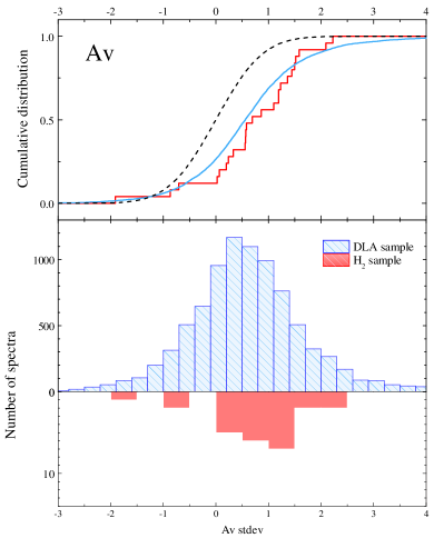
Figure 15: Distributions (bottom panel) and cumulative distributions (top panel) of the deviation (in unit of standard deviation) of $A_{V}$ compared to the mediam in the control samples. Red and blue colors correspond to the sample of H₂ bearing candidates and the whole DLA sample, respectively. The black dashed line in the top panel show the cumulative probability for a normal distribution. A similar excess is seen for the two samples.

6.3 Metal content

The measured equivalent widths (EW) of metal transitions can be used to characterize the metal content in DLA systems. We used EWs of C ii 1334 Å, Si ii 1526 Å, Fe ii 1608 Å, and Al iii 1670 Å  automatically measured in the DLA DR9 catalog (Noterdaeme et al., 2012). The distributions of EWs for DLA and H₂ candidate samples are shown in Fig. 16 and Fig. 17. Note, to construct cumulative distributions in Fig. 17 we used only spectra where metal lines are detected. It rejects most of possible false-positive DLA systems which presence in DLA DR9 sample. However, there can be a fraction of DLAs with low metal content, where some metal lines can’t be detected in SDSS spectra. Using Kolmogorov-Smirnov test we have found that EWs in the H₂ candidate sample is higher than EWs in DLA sample for C ii 1334 Å, Si ii 1526 Å  and Al iii 1670 Å   transitions at significance level 0.001, 0.039 and 0.014, respectively. On the other hand we have found that for Fe ii 1608 Å   transition distributions of H₂ candidate and DLA samples are not different at 0.94 significance level.

The overall excess in C ii, Si ii and Al iii EWs of the H₂ candidate sample over the DLA sample can possibly be interpreted as evidence for higher metal content. In such an interpretation the corresponding similarity of the Fe ii 1608 Å   EW distributions could reflect higher dust content in the H₂ bearing systems. However, EWs are not obviously related to column densities at low spectral resolution and large EWs could just be a consequence of larger velocity spread of the absorption. Note however that there is a correlation between velocity spread and metallicity (Ledoux et al., 2006) which would imply larger metallicities in the H₂ bearing candidates.

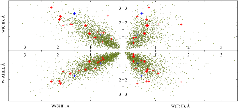
Figure 16: Equivalent widths of C ii, Si ii, Fe ii and Al iii absorptions. The green circles, red and blue crosses correspond to EWs for DLA systems detected in DR9, H₂ candidates and H₂ candidates confirmed by high resolution studies, respectively.

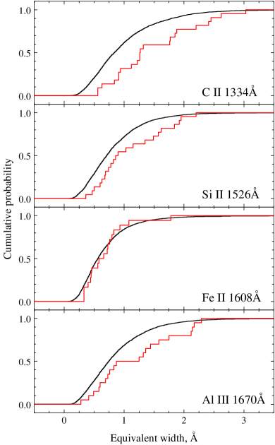
Figure 17: Cumulative distribution of equivalent widths of C ii, Si ii, Fe ii and Al iii absorptions. The black and red lines in each panel correspond for samples of DLA systems detected in DR9 and H₂ candidates, respectively.

7 Conclusion

We have performed a systematic search for H₂ absorption in DLAs detected towards quasars in the Sloan Digital Sky Survey releases DR7 and DR9. We have developed and used fully automatic procedures based on the profile fitting technique with modified $\chi^{2}$ function. The main difficulty of the search is the presence of the Ly-$\alpha$ forest which is dense at redshifts under consideration ($z>2.2$) and can effectively mimic H₂ absorption lines at the resolution and S/N of SDSS spectra. We carefully checked our searching procedure and found that it yields a completeness of $>99\%$ for $\log$N_H2 $>$18.5. However the number of false detections is rather high. For each of the candidates, the probability of false identification was calculated using two techniques. The first technique employs Monte-Carlo simulations to estimate the probability of an accidental fit of an absorption system in the Ly$\alpha$ forest. In this technique we used repeated random shifts for each H₂ absorption line in the particular spectrum. The advantage of this technique is to give an estimate of the false identification probability in the particular spectrum (i.e. the particular realization of the Ly$\alpha$ forest). The second technique uses a control sample to estimate the false identification probability. Control sample consists of the non-BAL non-DLA quasars from DR9 SDSS catalog which guarantees the absence of H₂ absorption systems. The false identification probability can be calculated as the identification rate of H₂ absorption systems in the control sample. We additionally have performed simulations of mock SDSS quasar spectra which were used to check the procedures and to increase statistics. We have found that the false identification probability depends on the H₂ column density and spectral properties, mainly on S/N, $z_{\rm QSO}$, and the number of H₂ absorption lines present in the spectrum. This method allows us to estimate the detection limit of H₂ absorption systems in SDSS spectra, i.e. the spectral properties for which the false identification probability is low and therefore the identification of the H₂ absorption system is robust. We found that in SDSS data a reasonable detection limit for H₂ column density, $\log$N${}_{\rm H_{2}}$, is higher than 19. We also derived that the upper limit on the fraction of DLAs with H₂ systems is statistically equal to 7 and 3% for, respectively, $\log$N${}_{\rm H_{2}}>$19 and 19.5. These are as upper limits because we tend to overestimate H₂ column densities. The false identification probabilities calculated by the Monte-Carlo sampling and control sample techniques agree with each other very well.

We have selected 23 candidates of H₂ absorption systems with high confidence level which are promising candidates for follow up high resolution studies. Taking into account the derived upper limit on the fraction of DLAs with saturated H₂ lines $\sim 7\%$ it leads us to the conclusion that only less than 3% of SDSS spectra are suitable for confident detection of H₂ absorption systems.

We studied the properties of these candidates, namely, color excess, extinction and equivalent widths of metal lines. There is a 1$\sigma$ $r-i$ color excess and no significant $A_{V}$ extinction in quasar spectra with an H2 candidate compared to standard DLA bearing quasar spectra. We find larger C ii, Si ii, and Al iii equivalent widths (EW) in the H₂ candidate sample over the DLA sample but no significant difference for Fe ii EWs. This is probably related to a larger spread in velocity of the absorption lines in the H₂ bearing sample and therefore possibly larger metallicities.

The selected candidates would increase by a factor of two the number of known H₂ absorption systems at high redshift. It is important to note, that we can confidently identify only saturated H₂ systems with high column densities, $\log$N${}_{\rm H_{2}}>19$. To date there are only a few such systems detected at high redshift. The selected candidates will undoubtedly allow us to gather a large sample of HD detections. The relative abundance of HD/H₂ molecules which provides important clues on the chemistry and star-formation history and also can be used to estimate the isotopic D/H ratio and consequently $\Omega_{b}$ – the density of baryonic matter in the Universe (Ivanchik et al., 2010; Balashev et al., 2010). In addition these systems are unique objects to search for CO molecule (Srianand et al., 2008). This molecule is suitable to estimate the physical conditions in interstellar clouds and the CMBR temperature at high redshift (Noterdaeme et al., 2010, 2011). We have selected four candidates with column densities $\log$N${}_{\rm H_{2}}>20$. Such systems have never been observed at high redshifts towards QSO sightlines and would provide an exclusive opportunity to study translucent clouds in the interstellar medium at high redshift.

Acknowledgments. We are very grateful the anonymous referee for the detailed and careful reading our manuscript and many useful comments. This work was partially supported by a State Program “Leading Scientific Schools of Russian Federation” (grant NSh-294.2014.2). SB and SK partially supported by the RF Presedent Programme (grant MK-4861.2013.2).

References

- Abazajian et al. (2009) Abazajian K. N. et al., 2009, Astrophys. Journal Suppl. Ser., 182, 543
- Ahn et al. (2012) Ahn C. P. et al., 2012, Astrophys. Journal Suppl. Ser., 203, 21
- Balashev et al. (2010) Balashev S. A., Ivanchik A. V., Varshalovich D. A., 2010, Astronomy Letters, 36, 761
- Busca et al. (2013) Busca N. G. et al., 2013, Astron. & Astrophys., 552, A96
- Crighton et al. (2013) Crighton N. H. M. et al., 2013, Mon. Not. of Royal Astron. Soc., 433, 178
- Cui et al. (2005) Cui J., Bechtold J., Ge J., Meyer D. M., 2005, Astrophys. Journal, 633, 649
- Ellison et al. (2001) Ellison S. L., Yan L., Hook I. M., Pettini M., Wall J. V., Shaver P., 2001, Astron. & Astrophys., 379, 393
- Fynbo et al. (2011) Fynbo J. P. U. et al., 2011, Mon. Not. of Royal Astron. Soc., 413, 2481
- Ge & Bechtold (1997) Ge J., Bechtold J., 1997, Astrophys. Journal Letters, 477, L73
- Guimarães et al. (2012) Guimarães R., Noterdaeme P., Petitjean P., Ledoux C., Srianand R., López S., Rahmani H., 2012, Astronomical Journal, 143, 147
- Ivanchik et al. (2005) Ivanchik A., Petitjean P., Varshalovich D., Aracil B., Srianand R., Chand H., Ledoux C., Boissé P., 2005, Astron. & Astrophys., 440, 45
- Ivanchik et al. (2010) Ivanchik A. V., Petitjean P., Balashev S. A., Srianand R., Varshalovich D. A., Ledoux C., Noterdaeme P., 2010, Mon. Not. of Royal Astron. Soc., 404, 1583
- Jorgenson et al. (2010) Jorgenson R. A., Wolfe A. M., Prochaska J. X., 2010, Astrophys. Journal, 722, 460
- Jorgenson et al. (2009) Jorgenson R. A., Wolfe A. M., Prochaska J. X., Carswell R. F., 2009, Astrophys. Journal, 704, 247
- Jorgenson et al. (2006) Jorgenson R. A., Wolfe A. M., Prochaska J. X., Lu L., Howk J. C., Cooke J., Gawiser E., Gelino D. M., 2006, Astrophys. Journal, 646, 730
- Krogager et al. (2012) Krogager J.-K., Fynbo J. P. U., Møller P., Ledoux C., Noterdaeme P., Christensen L., Milvang-Jensen B., Sparre M., 2012, Mon. Not. of Royal Astron. Soc., 424, L1
- Krühler et al. (2013) Krühler T. et al., 2013, ArXiv e-prints
- Krumholz (2012) Krumholz M. R., 2012, Astrophys. Journal, 759, 9
- Ledoux et al. (2003) Ledoux C., Petitjean P., Srianand R., 2003, Mon. Not. of Royal Astron. Soc., 346, 209
- Ledoux et al. (2006) Ledoux C., Petitjean P., Srianand R., 2006, Astrophys. Journal Letters, 640, L25
- Ledoux et al. (2002) Ledoux C., Srianand R., Petitjean P., 2002, Astron. & Astrophys., 392, 781
- Levshakov & Varshalovich (1985) Levshakov S. A., Varshalovich D. A., 1985, Mon. Not. of Royal Astron. Soc., 212, 517
- Malec et al. (2010) Malec A. L. et al., 2010, Mon. Not. of Royal Astron. Soc., 403, 1541
- Meiksin (2009) Meiksin A. A., 2009, Reviews of Modern Physics, 81, 1405
- Noterdaeme et al. (2008a) Noterdaeme P., Ledoux C., Petitjean P., Srianand R., 2008a, Astron. & Astrophys., 481, 327
- Noterdaeme et al. (2012) Noterdaeme P. et al., 2012, Astron. & Astrophys., 547, L1
- Noterdaeme et al. (2010) Noterdaeme P., Petitjean P., Ledoux C., López S., Srianand R., Vergani S. D., 2010, Astron. & Astrophys., 523, A80
- Noterdaeme et al. (2009) Noterdaeme P., Petitjean P., Ledoux C., Srianand R., 2009, Astron. & Astrophys., 505, 1087
- Noterdaeme et al. (2008b) Noterdaeme P., Petitjean P., Ledoux C., Srianand R., Ivanchik A., 2008b, Astron. & Astrophys., 491, 397
- Noterdaeme et al. (2011) Noterdaeme P., Petitjean P., Srianand R., Ledoux C., López S., 2011, Astron. & Astrophys., 526, L7
- Pâris et al. (2012) Pâris I. et al., 2012, Astron. & Astrophys., 548, A66
- Pâris et al. (2011) Pâris I. et al., 2011, Astron. & Astrophys., 530, A50
- Petitjean et al. (2006) Petitjean P., Ledoux C., Noterdaeme P., Srianand R., 2006, Astron. & Astrophys., 456, L9
- Prochaska et al. (2009) Prochaska J. X. et al., 2009, Astrophys. Journal Letters, 691, L27
- Prochaska & Wolfe (2009) Prochaska J. X., Wolfe A. M., 2009, Astrophys. Journal, 696, 1543
- Quider et al. (2011) Quider A. M., Nestor D. B., Turnshek D. A., Rao S. M., Monier E. M., Weyant A. N., Busche J. R., 2011, Astronomical Journal, 141, 137
- Rachford et al. (2002) Rachford B. L. et al., 2002, Astrophys. Journal, 577, 221
- Rahmani et al. (2013) Rahmani H. et al., 2013, ArXiv e-prints
- Reimers et al. (2003) Reimers D., Baade R., Quast R., Levshakov S. A., 2003, Astron. & Astrophys., 410, 785
- Schlafly & Finkbeiner (2011) Schlafly E. F., Finkbeiner D. P., 2011, Astrophys. Journal, 737, 103
- Schlegel et al. (1998) Schlegel D. J., Finkbeiner D. P., Davis M., 1998, Astrophys. Journal, 500, 525
- Schneider et al. (2010) Schneider D. P. et al., 2010, Astronomical Journal, 139, 2360
- Smee et al. (2013) Smee S. A. et al., 2013, Astronomical Journal, 146, 32
- Songaila et al. (1994) Songaila A. et al., 1994, Nature, 371, 43
- Srianand et al. (2008) Srianand R., Noterdaeme P., Ledoux C., Petitjean P., 2008, Astron. & Astrophys., 482, L39
- Srianand et al. (2000) Srianand R., Petitjean P., Ledoux C., 2000, Nature, 408, 931
- Srianand et al. (2005) Srianand R., Petitjean P., Ledoux C., Ferland G., Shaw G., 2005, Mon. Not. of Royal Astron. Soc., 362, 549
- Thompson (1975) Thompson R. I., 1975, Astrophys. Letters, 16, 3
- Vanden Berk et al. (2001) Vanden Berk D. E. et al., 2001, Astronomical Journal, 122, 549
- Varshalovich et al. (2001) Varshalovich D. A., Ivanchik A. V., Petitjean P., Srianand R., Ledoux C., 2001, Astronomy Letters, 27, 683
- Wendt & Molaro (2012) Wendt M., Molaro P., 2012, Astron. & Astrophys., 541, A69
- York et al. (2000) York D. G. et al., 2000, Astronomical Journal, 120, 1579
- Zhu & Ménard (2013) Zhu G., Ménard B., 2013, Astrophys. Journal, 770, 130