Restricted 3-body problem in effective-field-theory models of gravity

Abstract

One of the outstanding problems of classical celestial mechanics was the restricted $3$-body problem, in which a planetoid of small mass is subject to the Newtonian attraction of two celestial bodies of large mass, as it occurs, for example, in the sun-earth-moon system. On the other hand, over the last decades, a systematic investigation of quantum corrections to the Newtonian potential has been carried out in the literature on quantum gravity. The present paper studies the effect of these tiny quantum corrections on the evaluation of equilibrium points. It is shown that, despite the extreme smallness of the corrections, there exists no choice of sign of these corrections for which all qualitative features of the restricted $3$-body problem in Newtonian theory remain unaffected. Moreover, first-order stability of equilibrium points is characterized by solving a pair of algebraic equations of fifth degree, where some coefficients depend on the Planck length. The coordinates of stable equilibrium points are slightly changed with respect to Newtonian theory, because the planetoid is no longer at equal distance from the two bodies of large mass. The effect is conceptually interesting but too small to be observed, at least for the restricted $3$-body problems available in the solar system.

I Introduction

It is frequently the case, in physics, that an hybrid scheme, logically incomplete, turns out to be quite useful because the full theory is unknown or leads to equations that cannot be solved. Among the many conceivable examples of this feature, we mention the following, since they are relevant for motivating the research problem we are going to study. (i) The nonrelativistic particle in curved spacetime DeWitt2003 , where the Schrodinger equation is studied, which is part of nonrelativistic quantum theory, but the potential in such equation receives a contribution from spacetime curvature, which is instead defined and studied in general relativity. (ii) Quantum field theory in curved spacetime, where the right-hand side of the Einstein equations is replaced by the expectation value of the regularized and renormalized energy-momentum tensor $\langle T_{\mu\nu}\rangle$ evaluated in a classical spacetime geometry. Only at a subsequent stage does one try to consider the backreaction on the Einstein tensor, which, being coupled to a nonclassical object like $\langle T_{\mu\nu}\rangle$, cannot remain undisturbed. (iii) The application of the effective field theory point of view to the quantization of Einstein’s general relativity. Within this framework, starting from the Lagrangian density

$${\cal L}\equiv{\sqrt{-g}}\left[{c^{4}\over 16\pi G}R+{\cal L}_{{\rm matter}}\right],$$ (1)

one includes all possible higher derivative couplings of the fields in the gravitational Lagrangian. By doing so, any field singularities generated by loop diagrams can be associated with some component of the action and can be absorbed through a redefinition of the coupling constants of the theory. By treating all coupling coefficients as experimentally determined in this way, the effective field theory is finite and singularity-free at any finite order of the loop expansion D03 , even though it remains true that Einstein’s gravity is not perturbatively renormalizable DeWitt2003 and not even 2-loop on-shell finite Goroff1986 . (iv) Among the many outstanding problems of classical physics and, in particular, classical celestial mechanics, the 3-body problem played a major role, and the genius of Poincaré himself Poincare1890 was not enough to arrive at a complete solution. Nevertheless, one finds it often of interest, for example in the analysis of the Sun-Earth-Moon system, to consider the so-called restricted 3-body problem Pars . In this case a body $A$ of mass $\alpha$ and a body $B$ of mass $\beta<\alpha$ move under their mutual attraction. The center of mass $C$ of the $2$ bodies moves uniformly in a straight line, and one can suppose it to be at rest without loss of generality. The initial conditions tell us that the orbit of $B$ relative to $A$ is a circle, hence the orbit of each body relative to $C$ is a circle as well. Moreover, a third body, the planetoid $P$, moves in the plane of motion of $A$ and $B$. By hypothesis, $P$ is subject to the Newtonian attraction of $A$ and $B$, but its mass $m$ is so small that it cannot affect the motion of $A$ and $B$. The problem consists therefore in evaluating the motion of $P$.

Now when general relativity is viewed as an effective field theory, it becomes of interest to derive (at least) the leading classical and quantum corrections to the Newtonian potential of two large nonrelativistic masses. Hence we have been led to ask ourselves whether, despite the extremely small numbers involved, a quantum perspective on the restricted 3-body problem can be obtained. The question is not merely of academic interest. Indeed, on the one hand, we know already that very small quantities may produce nontrivial effects in physics. An example, among the many, is provided by the Stark effect: no matter how small is the external electric field, the Stark-effect Hamiltonian has absolutely continuous spectrum on the whole real line ReedSimon1978 , whereas the unperturbed Hamiltonian for hydrogen atom has discrete spectrum on the negative half-line. Yet another relevant example is provided by singular perturbations in quantum mechanics: if a one-dimensional harmonic oscillator is perturbed by a term proportional to negative powers of the position operator, then no matter how small is the weight coefficient one cannot recover the original Hamiltonian if the perturbation is switched off. The unperturbed Hamiltonian has in fact both even and odd eigenfunctions, whereas the singular perturbation enforces the stationary states to vanish at the origin, and the latter condition survives if the perturbation gets switched off Klauder , so that one eventually recovers a sort of ‘halved’ harmonic oscillator, with only half of the original eigenfunctions.

On the other hand, by virtue of the improved technology with respect to the golden age of Poincaré, it becomes conceivable to send off satellites in the solar system that, within our lifetime, might become part of suitable 3-body systems with the advantage, with respect to natural planetoids such as the moon, that the satellite can be ‘instructed’ to approach and even nearly miss the large masses of $A$ and $B$. Hence the putative quantum corrected Newtonian potential can be tested at very small distances, in circumstances which were inconceivable a century ago.

Section II builds the quantum-corrected Lagrangian of our model. Section III writes down the equilibrium conditions and the partial derivatives of our full potential up to the second order. Section IV is devoted to the equilibrium points on the line joining $A$ to $B$, while Sec. V studies equilibrium points not lying on the line that joins $A$ to $B$. Section VI identifies the unstable and stable equilibrium points. Concluding remarks and open problems are presented in Sec. VII.

II Quantum corrected Lagrangian of the model

Following Ref. Pars we take rotating axes with center of mass $C$ as origin, and $CB$ as axis of $x$ (see Fig. 1). The length $AB$ is denoted by $l$, and the angular velocity by $\omega$, so that

$$\omega^{2}={G(\alpha+\beta)\over l^{3}}.$$ (2)

By doing so, we choose to neglect any correction, either classical or quantum, to the Newtonian potential between the bodies having large mass. Thus, $A$ is permanently at rest, relative to the rotating axes, at the point of coordinates $(-a,0)$, and $B$ is permanently at rest at the point $(b,0)$, where Pars

$$a={\beta\over(\alpha+\beta)}l,\;b={\alpha\over(\alpha+\beta)}l.$$ (3)

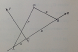
Figure 1: The figure shows the two bodies of large mass, $A$ and $B$, the center of mass $C$, and the planetoid at $P$.

The motion of the planetoid at $P(x,y)$ is the same as it would be if $A$ and $B$ were constrained to move as they do, hence the kinetic energy reads as

$$T={m\over 2}[({\dot{x}}-y\omega)^{2}+({\dot{y}}+x\omega)^{2}].$$ (4)

Furthermore, on denoting by $r$ the distance $AP$ and by $s$ the distance $BP$, i.e.

$$r^{2}=(x+a)^{2}+y^{2},\;s^{2}=(x-b)^{2}+y^{2},$$ (5)

the interaction potential is here taken to be

$$V=-{Gm\alpha\over r}\left(1+{k_{1}\over r}+{k_{2}\over r^{2}}\right)-{Gm\beta\over s}\left(1+{k_{3}\over s}+{k_{4}\over s^{2}}\right),$$ (6)

where, on denoting by $\kappa_{1},\kappa_{2},\kappa_{3}$ three dimensionless constants, one has

$$k_{1}=\kappa_{1}{G(m+\alpha)\over c^{2}},$$ (7)

$$k_{2}=k_{4}=\kappa_{2}{G\hbar\over c^{3}}=\kappa_{2}l_{P}^{2},$$ (8)

$$k_{3}=\kappa_{3}{G(m+\beta)\over c^{2}}.$$ (9)

In these formulas, $k_{1}$ and $k_{3}$ describe a classical (post-Newtonian) contribution, whereas $k_{2}=k_{4}$ describes a truly quantum correction. One arrives at these formulas through a rather involved Feynman-diagram analysis, and the $\kappa_{1},\kappa_{2},\kappa_{3}$ values obtained in Refs. D94 ; D03 differ both for the sign and their magnitude, because such References find

$$\kappa_{1}=3\;{\rm or}\;-1,$$ (10)

$$\kappa_{2}={41\over 10\pi}\;{\rm or}\;-{127\over 30\pi^{2}},$$ (11)

respectively. In Ref. D94 , the author evaluated all corrections resulting from vertex and vacuum polarization, whereas in Ref. D03 the authors considered all diagrams for a scattering process. However, if one needs to iterate the lowest order potential in some way, one should probably not include at least the box diagram. Thus, the result in Ref. D03 is closer to the full answer, but it depends on some of the details of how one is going to use it. We are grateful to the author of Ref. D94 for making all this clear to us.

Our quantum corrected Lagrangian is therefore assumed to take the form

$${L\over m} = {1\over 2}({\dot{x}}^{2}+{\dot{y}}^{2})+\omega(x{\dot{y}}-y{\dot{x}})+{1\over 2}\omega^{2}(x^{2}+y^{2})$$ (12)

$$+ {G\alpha\over r}\left(1+{k_{1}\over r}+{k_{2}\over r^{2}}\right)+{G\beta\over s}\left(1+{k_{3}\over s}+{k_{2}\over s^{2}}\right)$$

$$= T-V=T_{2}+T_{1}+T_{0}-V,$$

having denoted by $T_{n}$ the part of $T$ containing $n$-th order derivatives of $x$ or $y$. Such a Lagrangian does not depend on $t$ explicitly, and the Jacobi integral Pars for it exists and is given by

$$J=T_{2}+V-T_{0},$$ (13)

where, by virtue of (2.1) and (2.5),

$$T_{0}-V=GU,$$ (14)

having set

$$U\equiv{1\over 2}{(\alpha+\beta)\over l^{3}}(x^{2}+y^{2})+{\alpha\over r}\left(1+{k_{1}\over r}+{k_{2}\over r^{2}}\right)+{\beta\over s}\left(1+{k_{3}\over s}+{k_{2}\over s^{2}}\right).$$ (15)

The resulting Lagrange equations of motion read as

$${\ddot{x}}-2\omega{\dot{y}}=G{\partial U\over\partial x},$$ (16)

$${\ddot{y}}+2\omega{\dot{x}}=G{\partial U\over\partial y}.$$ (17)

Since, from (2.12) and (2.13), $J=T_{2}-GU$, one has the simple but nontrivial restriction according to which the motion of $P$ is only possible where

$$GU+J=T_{2}>0\Longrightarrow U>-{J\over G}.$$ (18)

III Equilibrium conditions and derivatives of the full potential

The equilibrium points, either stable or unstable, are points at which the full potential (2.14) is stationary, and hence one has to study its first and second partial derivatives. To begin, one finds

$${\partial U\over\partial x}=(\alpha+\beta){x\over l^{3}}-{\alpha(x+a)\over r^{3}}\left(1+2{k_{1}\over r}+3{k_{2}\over r^{2}}\right)-{\beta(x-b)\over s^{3}}\left(1+2{k_{3}\over s}+3{k_{2}\over s^{2}}\right).$$ (19)

Thus, on using (2.2) and defining (cf. the classical formulas in Ref. Pars )

$$\lambda\equiv{(\alpha+\beta)\over l^{3}}-{\alpha\over r^{3}}\left(1+2{k_{1}\over r}+3{k_{2}\over r^{2}}\right)-{\beta\over s^{3}}\left(1+2{k_{3}\over s}+3{k_{2}\over s^{2}}\right),$$ (20)

one can re-express ${\partial U\over\partial x}$ in the form (see Fig. 2)

$${\partial U\over\partial x}=\lambda x+{\alpha\beta l\over(\alpha+\beta)}\left[{1\over s^{3}}\left(1+2{k_{3}\over s}+3{k_{2}\over s^{2}}\right)-{1\over r^{3}}\left(1+2{k_{1}\over r}+3{k_{2}\over r^{2}}\right)\right],$$ (21)

while, with the same notation, the other first derivative reads as

$${\partial U\over\partial y}=\lambda y.$$ (22)

For this to vanish, it is enough that either $y$ or $\lambda$ vanishes, in complete formal analogy with the classical case Pars . When $y=0$, the equilibrium points lie on the line joining A to B, while the condition $\lambda=0$ yields the equilibrium points not lying on the line joining A to B. Second derivatives of $U$ and their sign are important to understand the nature of equilibrium points. For this purpose, we need the first derivatives of the function $\lambda$, which are found to be

$${\partial\lambda\over\partial x}={(x+a)\over r^{5}}\alpha\left(3+8{k_{1}\over r}+15{k_{2}\over r^{2}}\right)+{(x-b)\over s^{5}}\beta\left(3+8{k_{3}\over s}+15{k_{2}\over s^{2}}\right),$$ (23)

$${\partial\lambda\over\partial y}=y\left[{\alpha\over r^{5}}\left(3+8{k_{1}\over r}+15{k_{2}\over r^{2}}\right)+{\beta\over s^{5}}\left(3+8{k_{3}\over s}+15{k_{2}\over s^{2}}\right)\right],$$ (24)

by virtue of the identities (see (2.4))

$${\partial r\over\partial x}={(x+a)\over r},\;{\partial r\over\partial y}={y\over r},\;{\partial s\over\partial x}={(x-b)\over s},\;{\partial s\over\partial y}={y\over s}.$$ (25)

The second derivatives of $U$ are hence given by (see Figs. 3, 4 and 5)

$${\partial^{2}U\over\partial x^{2}}=\lambda+(x+a)^{2}{\alpha\over r^{5}}\left(3+8{k_{1}\over r}+15{k_{2}\over r^{2}}\right)+(x-b)^{2}{\beta\over s^{5}}\left(3+8{k_{3}\over s}+15{k_{2}\over s^{2}}\right),$$ (26)

$${\partial^{2}U\over\partial x\partial y}=y\left[{(x+a)\over r^{5}}\alpha\left(3+8{k_{1}\over r}+15{k_{2}\over r^{2}}\right)+{(x-b)\over s^{5}}\beta\left(3+8{k_{3}\over s}+15{k_{2}\over s^{2}}\right)\right],$$ (27)

$${\partial^{2}U\over\partial y^{2}}=\lambda+y^{2}\left[{\alpha\over r^{5}}\left(3+8{k_{1}\over r}+15{k_{2}\over r^{2}}\right)+{\beta\over s^{5}}\left(3+8{k_{3}\over s}+15{k_{2}\over s^{2}}\right)\right].$$ (28)

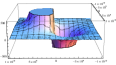
Figure 2: Plot of the partial derivative with respect to the $x$-coordinate of the potential $U(x,y)$ obtained by setting $\lambda=0$. The graph has been obtained with the choice of negative signs in (2.9) and (2.10) and for the system consisting of Jupiter and two of its satellites, i.e. Adrastea and Ganymede. For this system one has the following parameters: $\alpha=m_{\rm Jupiter}=1.90\times 10^{27}Kg$, $\beta=m_{\rm Ganymede}=1.48\times 10^{23}Kg$, $m=m_{\rm Adrastea}=7.5\times 10^{15}Kg$, $l=1.07\times 10^{9}$m, $a=8.33\times 10^{5}$m, $b=1.07\times 10^{9}$m.

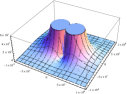
Figure 3: Plot of the partial derivative $U_{,xx}$ obtained by setting $\lambda=0$. The graph has been obtained with the choice of positive signs in (2.9) and (2.10) and for the system consisting of Sun, Earth and Moon. For this system one has the following parameters: $\alpha=m_{\rm Sun}=1.99\times 10^{30}Kg$, $\beta=m_{\rm Earth}=5.97\times 10^{24}Kg$, $m=m_{\rm Moon}=7.35\times 10^{22}Kg$, $l=1.50\times 10^{11}$m, $a=4.49\times 10^{5}$m, $b=1.49\times 10^{11}$m.

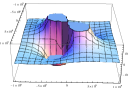
Figure 4: Plot of the partial derivative $U_{,xy}$ obtained by setting $\lambda=0$. The graph has been obtained with the choice of positive signs in (2.9) and (2.10) and for the system consisting of Jupiter and its satellites Adrastea and Ganymede.

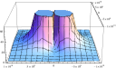
Figure 5: Plot of the partial derivative $U_{,yy}$ obtained by setting $\lambda=0$. The graph has been obtained with the choice of negative signs in (2.9) and (2.10) and for the system consisting of Sun, Earth and Moon.

IV Equilibrium points on the line joining $A$ to $B$

The line joining $A$ to $B$ is an axis having equation $y=0$, and it can be divided into 3 regions (see Figs. 6, 7 and 8):

$${\cal R}_{1}:\;x\in]-\infty,-a[,\;{\cal R}_{2}:\;x\in]-a,b[,\;{\cal R}_{3}:\;x\in]b,\infty[.$$

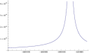
Figure 6: Plot of the potential $U(x,0)$ in the region ${\cal R}_{1}$. The graph has been obtained with the choice of positive signs in (2.9) and (2.10) and for the system consisting of Jupiter and its satellites Adrastea and Ganymede.

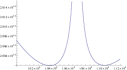
Figure 7: Plot of the potential $U(x,0)$ in the region ${\cal R}_{2}$. The graph has been obtained with the choice of positive signs in (2.9) and (2.10) and for the system consisting of Jupiter and its satellites Adrastea and Ganymede.

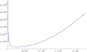
Figure 8: Plot of the potential $U(x,0)$ in the region ${\cal R}_{3}$. The graph has been obtained with the choice of positive signs in (2.9) and (2.10) and for the system consisting of Jupiter and its satellites Adrastea and Ganymede.

From Eq. (2.4) and $y=0$ one has $r=|x+a|,s=|x-b|$, and hence Eqs. (3.2) and (3.8) yield

$$\left.{\partial^{2}U\over\partial x^{2}}\right|_{y=0}=\left[{(\alpha+\beta)\over l^{3}}+2{\alpha\over r^{3}}+2{\beta\over s^{3}}\right]+2{\alpha\over r^{4}}\left(3k_{1}+6{k_{2}\over r}\right)+2{\beta\over s^{4}}\left(3k_{3}+6{k_{2}\over s}\right).$$ (29)

In Newtonian theory, since all terms in square brackets in (4.1) are positive, one concludes that $U_{,xx}$ is always positive on $y=0$. However, by virtue of (2.5)-(2.10), this may no longer be true in our case, if one adopts the negative signs on the right-hand side of (2.9) and (2.10) and if one lets either $r$ or $s$ or both to approach $0$. Thus, the sufficient condition for preservation of the sign in Newtonian theory reads as

$$\boxed{\left(3k_{1}+6{k_{2}\over r}\right)+{\beta\over\alpha}\left({r\over s}\right)^{4}\left(3k_{3}+6{k_{2}\over s}\right)>0},$$ (30)

which is however violated with the choice of negative signs in (2.9) and (2.10).

Note that the function $U(x,0)$ has, from (2.14), the limiting behavior

$$\lim_{x\to-a}U(x,0)=\lim_{x\to b}U(x,0)=+\infty,$$ (31)

$$\lim_{x\to-\infty}U(x,0)=\lim_{x\to+\infty}U(x,0)=+\infty.$$ (32)

Moreover, $U_{,x}$ passes just once through $0$ in each of the $3$ regions ${\cal R}_{1},{\cal R}_{2}$ and ${\cal R}_{3}$, which implies that there exist $3$ equilibrium points on $AB$, when $U$ has minima at the points $N_{1}(x=n_{1}),N_{2}(x=n_{2})$ and $N_{3}(x=n_{3})$.

To study the location of the equilibrium points, we note, following Ref. Pars , that

$${r\over(x+a)}=(-1,1,1),\;{s\over(x-b)}=(-1,-1,1),$$ (33)

the $3$ values on the right-hand side referring to ${\cal R}_{1},{\cal R}_{2}$ and ${\cal R}_{3}$, respectively, so that in ${\cal R}_{1}$ for example (see (3.3))

$${\partial U\over\partial x}=(\alpha+\beta){x\over l^{3}}+{\alpha\over r^{2}}\left(1+2{k_{1}\over r}+3{k_{2}\over r^{2}}\right)+{\beta\over s^{2}}\left(1+2{k_{3}\over s}+3{k_{2}\over s^{2}}\right).$$ (34)

At the point $x=-a-l$ one has $r=l,s=2l$, and from (2.2) and (4.6) one finds

$$\left.{\partial U\over\partial x}\right|_{x=-a-l}=-{7\over 4}{\beta\over l^{2}}+{1\over l^{3}}\left[\alpha\left(2k_{1}+3{k_{2}\over l}\right)+{\beta\over 4}\left(k_{3}+{3\over 4}{k_{2}\over l}\right)\right].$$ (35)

In Newtonian theory, the sum in square brackets in (4.7) is absent and one can say that $U_{,x}$ is negative and hence $N_{1}$ lies between $x=-a-l$ and $x=-a$. In our model, for this to remain true, one should impose the sufficient condition

$$\boxed{2k_{1}+3{k_{2}\over l}+{\beta\over 4\alpha}\left(k_{3}+{3\over 4}{k_{2}\over l}\right)<0},$$ (36)

which is however violated with the choice of positive signs in (2.9) and (2.10).

Similarly, to understand whether the equilibrium point $N_{2}$ lies between $C$ and $B$, one has to evaluate $U_{,x}$ at $C$, where $r=a,s=b,x=y=0$, which yields, from (3.3),

$$\left.{\partial U\over\partial x}\right|_{C}=-(\alpha^{3}-\beta^{3}){(\alpha+\beta)^{2}\over\alpha^{2}\beta^{2}l^{2}}-\left[{\alpha\over a^{3}}\left(2k_{1}+3{k_{2}\over a}\right)+{\beta\over b^{3}}\left(2k_{3}+3{k_{2}\over b}\right)\right].$$ (37)

In Newtonian theory, the sum in square brackets in (4.9) does not occur, and hence $\left.{\partial U\over\partial x}\right|_{C}$ is always negative. For this to remain true in our model, one has to impose the sufficient condition

$$\boxed{k_{1}+{3\over 2}{k_{2}\over a}+{\beta\over\alpha}\left({a\over b}\right)^{3}\left(k_{3}+{3\over 2}{k_{2}\over b}\right)>0},$$ (38)

which is instead violated with the choice of negative signs in (2.9) and (2.10).

At this stage, despite the incompleteness of our analysis, we have already proved a simple but nontrivial result: not only can our model be used to discriminate among competing theories of effective gravity, but there exists no choice of signs in (2.9) and (2.10) for which all qualitative features of the restricted $3$-body problem in Newtonian theory remain unaffected. As far as we can see, this means that either we reject effective theories of gravity or we should expect them to be able to lead to testable effects in suitable $3$-body systems, e.g. a satellite which is programmed to approach very closely (much closer than the moon can afford approaching the earth) $2$ celestial bodies of large mass.

Furthermore, from (3.10) we find

$$\left.{\partial^{2}U\over\partial y^{2}}\right|_{N_{1}}=\lambda={\alpha\beta l\over(\alpha+\beta)}{1\over x}\left({1\over r^{3}}-{1\over s^{3}}\right)$$ (39)

$$+ {1\over x}\left[2\left({k_{1}\over r^{4}}-{k_{3}\over s^{4}}\right)+3k_{2}\left({1\over r^{5}}-{1\over s^{5}}\right)\right].$$

In Newtonian theory, the sum of terms in square brackets in (4.11) does not occur, and hence one points out that, since at $N_{1}$ $x$ is negative and $r<s$, the second derivative of $U$ at $N_{1}$ is negative Pars . In our model, however, the sufficient condition for this to remain true, i.e.

$$\boxed{\left({k_{1}\over r^{4}}-{k_{3}\over s^{4}}\right)+{3\over 2}k_{2}\left({1\over r^{5}}-{1\over s^{5}}\right)>0},$$ (40)

can be violated, for example, as $r\rightarrow 0$ with the negative choice of sign in (2.10).

We note also that at $N_{2}$, where $r=x+a$ and $s=x-b$, one has from (3.10)

$$\left.{\partial^{2}U\over\partial y^{2}}\right|_{N_{2}}={(\alpha+\beta)\over l^{3}}-{\alpha\over r^{3}}-{\beta\over s^{3}}-\left[2\left(\alpha{k_{1}\over r^{4}}+\beta{k_{3}\over s^{4}}\right)+3k_{2}\left({\alpha\over r^{5}}+{\beta\over s^{5}}\right)\right].$$ (41)

In Newtonian theory, the sum of terms in square brackets in (4.13) does not occur, and one finds that $U_{,yy}$ is negative at $N_{2}$, because in ${\cal R}_{2}$ both $r$ and $s$ are less than $l$. In our model, for this to remain true, the following sufficient condition should hold:

$$\boxed{\alpha{k_{1}\over r^{4}}+\beta{k_{3}\over s^{4}}+{3\over 2}k_{2}\left({\alpha\over r^{5}}+{\beta\over s^{5}}\right)>0},$$ (42)

which is however violated if the negative signs are chosen in (2.9) and (2.10).

On reverting now to the graph of $U(x,0)$, there are minima at $N_{1},N_{2}$ and $N_{3}$, and we would like to determine at which of these $3$ points $U(x,0)$ has the greatest value, and at which it has instead the least value. In Newtonian theory, one finds that $U(n_{2})>U(n_{3})>U(n_{1})$. To establish the counterpart in our model, let $Q_{3}(x=q_{3})$ be the point of ${\cal R}_{3}$ whose distance from $B$ is equal to the distance of $N_{2}$ from $B$, i.e. $N_{2}B=BQ_{3}=j$. Thus, following patiently a number of cancellations, we find

$$U(n_{2})-U(q_{3})=U(x=b-j,y=0,r=l-j,s=j)$$ (43)

$$- U(x=b+j,y=0,r=l+j,s=j)$$

$$= 2\alpha j\left({1\over(l-j)^{2}}-{1\over l^{2}}\right)$$

$$+ {2\alpha j\over(l-j)^{2}(l+j)^{2}}\left[2k_{1}l+{k_{2}(j^{2}+3l^{2})\over(l^{2}-j^{2})}\right].$$

In Newtonian theory, the sum of terms in square brackets in (4.15) does not occur, and one therefore finds $U(n_{2})-U(q_{3})>0$. In our model, for this to remain true, one should impose the following sufficient condition

$$\boxed{k_{1}+{1\over 2}k_{2}{(j^{2}+3l^{2})\over l(l^{2}-j^{2})}>0},$$ (44)

which is instead violated if the negative signs are chosen in (2.9) and (2.10).

Last, let $Q_{1}(x=q_{1})$ be the point of ${\cal R}_{1}$ whose distance from $C$ is equal to the distance of $N_{3}$ from $C$, i.e. $Q_{1}C=CN_{3}=f$. Then we find

$$U(n_{3})-U(q_{1})=U(x=f,y=0,r=x+a,s=x-b)$$ (45)

$$- U(x=-f,y=0,r=x-a,s=-x+b)$$

$$= {2\alpha\beta l(b^{2}-a^{2})\over(\alpha+\beta)(f^{2}-a^{2})(f^{2}-b^{2})}$$

$$+ {2\alpha\beta l\over(\alpha+\beta)(f^{2}-a^{2})^{2}(f^{2}-b^{2})^{2}}\biggr{\{}2f\Bigr{[}k_{3}(f^{2}-a^{2})^{2}-k_{1}(f^{2}-b^{2})^{2}\Bigr{]}$$

$$+ {k_{2}\Bigr{[}(b^{2}+3f^{2})(f^{2}-a^{2})^{3}-(a^{2}+3f^{2})(f^{2}-b^{2})^{3}\Bigr{]}\over(f^{2}-a^{2})(f^{2}-b^{2})}\biggr{\}}.$$

In Newtonian theory, the sum of terms in curly brackets in (4.17) does not occur, and one finds $U(n_{3})>U(q_{1})$. In our model, for this to remain true, one should impose the sufficient condition

$$\boxed{2f\Bigr{[}k_{3}(f^{2}-a^{2})^{2}-k_{1}(f^{2}-b^{2})^{2}\Bigr{]}+{k_{2}\Bigr{[}(b^{2}+3f^{2})(f^{2}-a^{2})^{3}-(a^{2}+3f^{2})(f^{2}-b^{2})^{3}\Bigr{]}\over(f^{2}-a^{2})(f^{2}-b^{2})}>0}.$$ (46)

This is more involved than (4.16), and it is not a priori so obvious whether a choice of signs in (2.9) and (2.10) leads always to its fulfillment.

V Equilibrium points not lying on the line that joins $A$ to $B$

When the equilibrium points do not lie on the line joining $A$ to $B$, the coordinate $y$ does not vanish and hence the first derivative (3.4) vanishes because $\lambda=0$. On the other hand, the first derivative (3.3) should vanish as well, which then implies, by virtue of $\lambda=0$,

$${1\over r^{3}}\left(1+2{k_{1}\over r}+3{k_{2}\over r^{2}}\right)={1\over s^{3}}\left(1+2{k_{3}\over s}+3{k_{2}\over s^{2}}\right).$$ (47)

Unlike Newtonian theory Pars , this equation is no longer solved by $r=s$. The definition (3.2), jointly with (5.1), makes it now possible to express the condition $\lambda=0$ in the form

$${1\over l^{3}}={1\over r^{3}}+2{k_{1}\over r^{4}}+3{k_{2}\over r^{5}}.$$ (48)

This is an algebraic equation of fifth degree in the variable

$$w\equiv{1\over r},$$ (49)

and we divide both sides by $3k_{2}$ and exploit the definitions (2.6)-(2.8) to write it in the form

$$\sum_{k=0}^{5}\zeta_{k}w^{k}=0,$$ (50)

where

$$\zeta_{5}\equiv 1,$$ (51)

$$\zeta_{4}\equiv{2\over 3}{\kappa_{1}\over\kappa_{2}}{G(m+\alpha)\over c^{2}l_{P}^{2}},$$ (52)

$$\zeta_{3}\equiv{1\over 3\kappa_{2}}{1\over l_{P}^{2}},$$ (53)

$$\zeta_{2}=\zeta_{1}\equiv 0,$$ (54)

$$\zeta_{0}\equiv-{1\over 3\kappa_{2}}{1\over l_{P}^{2}l^{3}}.$$ (55)

Since this equation is of odd degree with real coefficients, the fundamental theorem of algebra guarantees the existence of at least a real solution, despite the lack of a general solution algorithm for all algebraic equations of degree greater than $4$. Moreover, by virtue of the small term ${G\over c^{2}}$, the coefficient $\zeta_{4}$ plays a negligible role both in the sun-earth-moon system, where $\alpha=m_{{\rm sun}},\beta=m_{{\rm earth}},m=m_{{\rm moon}},l=l_{{\rm sun-earth}}$, and in many other conceivable toy models of the restricted $3$-body problem, as is confirmed by detailed numerical checks. We find only one positive root $w_{+}(l)$ of Eq. (5.4) when the positive signs are chosen in (2.9) and (2.10), following D03 (whereas $2$ positive roots are obtained when negative signs are taken in (2.9) and (2.10)), from which $r(l)={1\over w_{+}(l)}$. Eventually, one can evaluate $s(l)=s(r(l))$ from Eq. (5.1), which can be viewed as an algebraic equation of fifth degree in the variable

$$u\equiv{1\over s},$$ (56)

i.e. (cf. Eq. (5.4))

$$\sum_{k=0}^{5}{\widetilde{\zeta}}_{k}u^{k}=0,$$ (57)

where

$${\widetilde{\zeta}}_{k}=\zeta_{k}\;\forall k=0,1,2,3,5,$$ (58)

$${\widetilde{\zeta}}_{4}\equiv{2\over 3}{\kappa_{3}\over\kappa_{2}}{G(m+\beta)\over c^{2}l_{P}^{2}}.$$ (59)

Also in the case of Eq. (5.11) we have found only a positive solution $u_{+}(l)$ both for the sun-earth-moon system and for any conceivable toy model for this restricted $3$-body problem.

The Cartesian coordinates $(x,y)$ of the equilibrium points not lying along $AB$ can be found from the general formulas (2.4), with the notation

$$r(l)\equiv{1\over w_{+}(l)},\;s(l)\equiv{1\over u_{+}(l)},$$ (60)

i.e.

$$r^{2}(l)=x^{2}+y^{2}+2ax+a^{2},$$ (61)

$$s^{2}(l)=x^{2}+y^{2}-2bx+b^{2}.$$ (62)

Subtraction of Eq. (5.16) from Eq. (5.15) yields

$$x(l)\equiv{(r^{2}(l)-s^{2}(l)+b^{2}-a^{2})\over 2(a+b)},$$ (63)

while $y(l)$ can be obtained from (5.15) in the form

$$y_{\pm}(l)\equiv\pm\sqrt{r^{2}(l)-x^{2}(l)-2ax(l)-a^{2}}.$$ (64)

Thus, there exist $2$ equilibrium points not lying on the line joining $A$ to $B$, hereafter written in the form

$$N_{4}(x(l),y_{+}(l)),\;N_{5}(x(l),y_{-}(l)).$$ (65)

In Newtonian theory, where $r=s$, the formula (5.19) reduces to the familiar Pars

$$N_{4}\left({(\alpha-\beta)\over(\alpha+\beta)}{l\over 2},{\sqrt{3}\over 2}l\right),\;N_{5}\left({(\alpha-\beta)\over(\alpha+\beta)}{l\over 2},-{\sqrt{3}\over 2}l\right),$$ (66)

by virtue of (2.2). The geometric interpretation of these formulas is simple but it has a nontrivial consequence: at the points $N_{4}$ and $N_{5}$ the planetoid is not at the same distance from $A$ and $B$, unlike Newtonian theory. Our quantum corrected model predicts a very tiny displacement from the case $r=s$, but its effect cannot be observed in the solar system, because in the available implementations of the restricted $3$-body problem the differences

$$\delta_{1}(l)\equiv x(l)-{(\alpha-\beta)\over(\alpha+\beta)}{l\over 2},\;\delta_{2}(l)\equiv y_{+}(l)-{\sqrt{3}\over 2}l,\;\delta_{3}(l)\equiv y_{-}(l)+{\sqrt{3}\over 2}l$$ (67)

are too small to be observed, as is unfortunately the case for many interesting effects in quantum gravity.

VI Unstable and stable equilibrium points

A rather important question is whether the positions of equilibrium are stable. In the affirmative case, the planetoid would therefore remain permanently near the point of stable equilibrium. To study this issue, on denoting by $(x_{0},y_{0})$ one of the points $N_{1},N_{2},N_{3},N_{4},N_{5}$, one writes in the equations of motion (2.15) and (2.16)

$$x=x_{0}+\xi,\;y=y_{0}+\eta.$$ (68)

By expanding the right-hand sides in powers of $\xi$ and $\eta$, and retaining only terms of first order, one obtains the linear approximation Pars

$${\ddot{\xi}}-2\omega{\dot{\eta}}=G(A\xi+B\eta),$$ (69)

$${\ddot{\eta}}+2\omega{\dot{\xi}}=G(B\xi+C\eta),$$ (70)

having defined

$$A\equiv\left.{\partial^{2}U\over\partial x^{2}}\right|_{x_{0},y_{0}},\;B\equiv\left.{\partial^{2}U\over\partial x\partial y}\right|_{x_{0},y_{0}},\;C\equiv\left.{\partial^{2}U\over\partial y^{2}}\right|_{x_{0},y_{0}}.$$ (71)

Equations (6.2) and (6.3) are a coupled set of ordinary differential equations with constant coefficients, and hence one can look for its solution in the form

$$\xi=\xi_{0}{\rm e}^{{t\over\tau}},\;\eta=\eta_{0}{\rm e}^{{t\over\tau}}.$$ (72)

This leads to the linear homogeneous system of algebraic equations

$$\left({1\over\tau^{2}}-GA\right)\xi-\left(2{\omega\over\tau}+GB\right)\eta=0,$$ (73)

$$\left(2{\omega\over\tau}-GB\right)\xi+\left({1\over\tau^{2}}-GC\right)\eta=0.$$ (74)

Nontrivial solutions exist if and only if the determinant of the matrix of coefficients vanishes. Such a condition is expressed by the algebraic equation of fourth degree

$${1\over\tau^{4}}-[G(A+C)-4\omega^{2}]{1\over\tau^{2}}+G^{2}(AC-B^{2})=0.$$ (75)

The variable is of course the square of ${1\over\tau}$, and for it one finds, from the standard theory of algebraic equations of second degree,

$${1\over\tau^{2}}={1\over 2}[G(A+C)-4\omega^{2}]\pm{1\over 2}\sqrt{(G(A+C)-4\omega^{2})^{2}-4G^{2}(AC-B^{2})}.$$ (76)

VI.1 Conditions for first-order instability of $N_{1},N_{2},N_{3}$

In Newtonian theory, $(AC-B^{2})$ is negative at $N_{1},N_{2},N_{3}$, and hence only half of the ${1\over\tau^{2}}$ values are negative, which implies that the criterion for first-order stability Pars is not satisfied. In our model, it remains true, from (3.9), that our $B$ vanishes at $N_{1},N_{2},N_{3}$, and we express our $A$ at $N_{1},N_{2},N_{3}$ from (4.1), our $C$ at $N_{1},N_{3}$ from (4.11), and our $C$ at $N_{2}$ from (4.13). Thus, provided that the sufficient conditions (4.2), (4.12) and (4.14) hold, which are in turn guaranteed, as we know, from the choice of positive signs in (2.9) and (2.10), it is always true that $(AC-B^{2})<0$, and the points $N_{1},N_{2},N_{3}$ remain points of unstable equilibrium even in the presence of quantum corrections obtained from an effective-gravity picture D03 .

VI.2 Conditions for first-order stability of $N_{4},N_{5}$

At the points $N_{4}$ and $N_{5}$, the vanishing of $\lambda$ simplifies the evaluation of $A$ and $C$ from (3.8) and (3.10), and we find (with the understanding that $r=r(l)$, $s=s(l)$ and $y=y(l)$ as in Sec. V)

$$A={\alpha(r^{2}-y^{2})\over r^{5}}\left(3+8{k_{1}\over r}+15{k_{2}\over r^{2}}\right)+{\beta(s^{2}-y^{2})\over s^{5}}\left(3+8{k_{3}\over s}+15{k_{2}\over s^{2}}\right),$$ (77)

$$C={\alpha y^{2}\over r^{5}}\left(3+8{k_{1}\over r}+15{k_{2}\over r^{2}}\right)+{\beta y^{2}\over s^{5}}\left(3+8{k_{3}\over s}+15{k_{2}\over s^{2}}\right),$$ (78)

$$B^{2} = {\alpha^{2}y^{2}(r^{2}-y^{2})\over r^{10}}\left(3+8{k_{1}\over r}+15{k_{2}\over r^{2}}\right)^{2}+{\beta^{2}y^{2}(s^{2}-y^{2})\over s^{10}}\left(3+8{k_{3}\over s}+15{k_{2}\over s^{2}}\right)^{2}$$ (79)

$$+ {2\alpha\beta y^{2}\over r^{5}s^{5}}\left(3+8{k_{1}\over r}+15{k_{2}\over r^{2}}\right)\left(3+8{k_{3}\over s}+15{k_{2}\over s^{2}}\right)(x^{2}+(a-b)x-ab).$$

In the evaluation of $(AC-B^{2})$ we find therefore exact cancellation of the $2$ pairs of terms involving $\alpha^{2}$ and $\beta^{2}$. Moreover, on exploiting from (2.4) the identity

$$r^{2}+s^{2}=2(x^{2}+y^{2})+2(a-b)x+a^{2}+b^{2},$$ (80)

we obtain, bearing in mind that $(a+b)=l$,

$$(AC-B^{2})={\alpha\beta y^{2}l^{2}\over r^{5}s^{5}}\left(3+8{k_{1}\over r}+15{k_{2}\over r^{2}}\right)\left(3+8{k_{3}\over s}+15{k_{2}\over s^{2}}\right).$$ (81)

This is all we need, because it is clearly positive if the positive signs are chosen in (2.9) and (2.10), and it ensures that all values of ${1\over\tau^{2}}$ from the solution formula (6.9) are negative (a result further confirmed by numerical analysis for the sun-earth-moon and Jupiter-Adrastea-Ganymede systems), in full agreement with the criterion for first-order stability Pars of the equilibrium points.

VII Concluding remarks and open problems

Not only has the (restricted) $3$-body problem played an important role in the historical development of celestial mechanics Poincare1890 ; Poincare1892 and classical dynamics Pars , but it has also found important applications to modern physics. For example, in Ref. Bial94 , the authors have discovered, by analytic and numerical methods, the existence of stable, although nonstationary, quantum states of electrons moving on circular orbits that are trapped in an effective potential well made of the Coulomb potential and the rotating electric field produced by a strong circularly polarized electromagnetic wave.

In the theory of gravitation, the undisputable smallness of classical and quantum corrections to the Newtonian potential had always discouraged the investigation of their role in the restricted $3$-body problem. Our contribution has been precisely a systematic investigation of the ultimate consequences of such additional terms. Our sufficient conditions (4.2), (4.8), (4.10), (4.12), (4.14), (4.16) and (4.18) are original and imply that some changes of qualitative features are unavoidable with respect to Newtonian theory, regardless of the choice of signs made in (2.9) and (2.10), although $6$ out of $7$ sufficient conditions are fulfilled with the choice of positive signs in (2.9) and (2.10). Section V has shown that the equilibrium points not lying on the line that joins $A$ to $B$ are found by solving a pair of algebraic equations of fifth degree, and their coordinates have been obtained for the first time in the class of effective theories of gravity studied in Refs. D03 ; D94 . Section VI has studied first-order stability for the $5$ equilibrium points of the problem. We have proved therein that, provided the positive signs are chosen in (2.9) and (2.10), the $3$ points along the line joining $A$ to $B$ are unstable, while the $2$ points not on $AB$ are stable equilibrium points to first order.

It now remains to be seen whether the present techniques in space sciences make it possible to realize a satellite $P$ that approaches so closely the celestial bodies $A$ and $B$ that our tiny corrections start making themselves manifest. Unfortunately, the differences in (5.21) between quantum corrected and Newtonian values of the coordinates of stable-equilibrium points $N_{4}$ and $N_{5}$ are too small to be observed, at least in the solar system. However, one cannot yet rule out that future technological developments will make it possible to ckeck against observations the current effective theories of gravity, which would bring quantum gravity research much closer to the experimental world. Last, but not least, the whole analysis performed in Refs. Poincare1890 ; Poincare1892 , if generalized to the extended theories of gravity inspired by the works in Refs. D94 ; D03 , might lead to the discovery of novel features of orbital motion.

- (1) B. S. DeWitt, The Global Approach to Quantum Field Theory, International Series of Monographs on Physics 114 (Clarendon Press, Oxford, 2003).
- (2) N. E. J. Bjerrum-Bohr, J. F. Donoghue, and B. R. Holstein, Phys. Rev. D 67, 084033 (2003).
- (3) M. Goroff and A. Sagnotti, Nucl. Phys. B 266, 709 (1986).
- (4) H. Poincaré, Acta Mathematica 13, 1 (1890); Bull. Astronomique 8, 12 (1891).
- (5) L. A. Pars, A Treatise on Analytical Dynamics (Heinemann, London, 1965).
- (6) M. Reed and B. Simon, Methods of Modern Mathematical Physics. IV: Analysis of Operators (Academic Press, New York, 1978).
- (7) J. Klauder, Beyond Conventional Quantization (Cambridge University Press, Cambridge, 2000).
- (8) J. F. Donoghue, Phys. Rev. Lett. 72, 2996 (1994).
- (9) H. Poincaré, Les Methodes Nouvelles de la Mecanique Celeste (Gauthier-Villars, Paris, 1892).
- (10) I. Bialynicki-Birula, M. Kalinski, and J. H. Eberly, Phys. Rev. Lett. 73, 1777 (1994).