Laser beam complex amplitude measurement by phase diversity

Abstract

The control of the optical quality of a laser beam requires a complex amplitude measurement able to deal with strong modulus variations and potentially highly perturbed wavefronts. The method proposed here consists in an extension of phase diversity to complex amplitude measurements that is effective for highly perturbed beams. Named camelot for Complex Amplitude MEasurement by a Likelihood Optimization Tool, it relies on the acquisition and processing of few images of the beam section taken along the optical path. The complex amplitude of the beam is retrieved from the images by the minimization of a Maximum a Posteriori error metric between the images and a model of the beam propagation. The analytical formalism of the method and its experimental validation are presented. The modulus of the beam is compared to a measurement of the beam profile, the phase of the beam is compared to a conventional phase diversity estimate. The precision of the experimental measurements is investigated by numerical simulations.

Office National d’Etudes et de Recherches Aérospatiales (ONERA)
High Angular Resolution Unit, Optics Department,
29 avenue de la division Leclerc
92332 Châtillon, FRANCE

^∗nicolas.vedrenne@onera.fr

(140.3295) Laser beam characterization; (280.4788) Optical sensing and sensors; (010.7350) Wave-front sensing; (100.3190) Inverse problems; (100.5070) Phase retrieval.

1 Introduction

The optical quality of the beam is a critical issue for intense lasers: a good optical quality is necessary to optimize stimulated amplification in optical amplifiers, to prevent optical surfaces from deteriorating due to hot spots, and to optimize the flux density at focus. For these reasons the optical quality of the beams of intense lasers must be monitored. To this end, wavefront analysis has to cope with the presence of high spatial frequencies in the beam profile due to speckle patterns. Commonly used wavefront sensors, whether Shack-Hartmann [1] (SH) or shearing interferometers [2], rely on the assumption of a continuous phase structure. In order to measure high spatial frequencies, the sampling of the wavefront has to be fine. This requires additional optical components and many measurement points, which are manageable assuming large focal plane sensors. Moreover, these concepts require the reconstruction of the wavefront from wavefront gradient measurements. The reconstruction process is only valid if the wavefront is continuous and can be measured on a domain that is a connected set in the topological sense.

To bypass the above limitations, far field wavefront sensing techniques such as Phase Diversity are an appealing alternative. Phase Diversity, i.e., the recovery of the field from a set of intensity distributions in planes transverse to propagation, is a well-established method. The vast majority of the work on this technique has concentrated on the estimation of the phase for applications related to imaging, assuming that the modulus is known, as is often reasonable in astronomy at least—see in particular [3, 4] for seminal contributions, [5] for a review on phase diversity, and [6] for an application of phase diversity to reach the diffraction limit with Strehl Ratios as high as 98.7%.

Yet, with intense lasers, the wave profile may present strong spatial variations [7]. For this reason, in this application of phase diversity one needs to estimate the complex amplitude. Early work on phase and modulus estimation was performed for the characterization of the Hubble Space Telescope (HST). Roddier [8] obtained non-binary pupil modulus images using an empirical procedure combining several Gerchberg-Saxton (GS) type algorithms [9], while Fienup [10] used a metric minimization approach [11] to estimate the binary pupil shape, parametrized through the shift of the camera obscuration.

The GS algorithm belongs to a larger class of methods based on successive mathematical projections, studied in [12]. Although there is a connection between projection-based algorithms and the minimization of a least-square functional of the unknown wavefront [13], the use of an explicit metric to be optimized is often preferable to projection-based algorithms for several reasons. Firstly, it allows the introduction of more unknowns (differential tip-tilts between images, a possibly extended object, etc); secondly, it allows the incorporation of prior knowledge about the statistics of the noise and/or of the sought wavefront; thirdly, projection based algorithms are often prone to stagnation.

The first work on estimating a wave complex amplitude from phase diversity data with an explicit metric along with experimental results was published by Jefferies [14], in view of incoherent image reconstruction in a strong perturbation regime. The authors encountered difficulties in the metric minimization, which may in part be due to the parametrization of the complex amplitude with its polar form rather than its rectangular one. Experimental results in a strong perturbation regime have also been obtained by Almoro et al. [15] using a wave propagation-based algorithm. This algorithm, which can be interpreted as successive mathematical projections [12], required many measurements recorded at axially-displaced detector planes. The said technique was adapted for smooth test object wavefronts using a phase diffuser and, for single plane detection, with a spatial light modulator[16]. More recently, Thurman and Fienup [17] studied, through numerical simulations, the influence of under-sampling in the reconstruction of a complex amplitude from phase diversity data with an explicit metric optimization, in view of estimating the pupil modulus and aberrations of a segmented telescope, but this metric was not derived from the data likelihood.

This paper aims at presenting a likelihood-based complex amplitude retrieval method relying on phase diversity and requiring few images, together with an experimental validation. As in [17], the complex amplitude is described by its rectangular form rather than the polar one to make the optimization more efficient. The method, named camelot for Complex Amplitude Measurement by a Likelihood Optimization Tool, is described in Section 2. In Section 3 we validate it experimentally and assess its performance on a laboratory set-up designed to shape the complex amplitude of a laser beam and record images of the focal spot at several longitudinal positions. In particular, a cross-validation with conventional phase diversity is presented. Finally, experimental results are confronted to carefully designed simulations taking into account many error sources in Section 4. In particular, the impact of photon, detector and quantization noises on the estimation precision is studied.

2 camelot

2.1 Problem statement

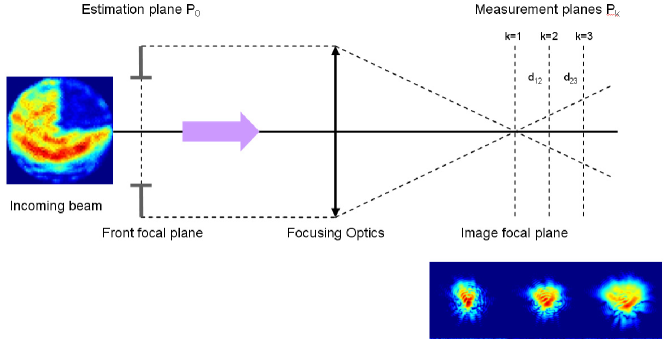
Figure 1: Schematic diagram for phase diversity measurement.

The schematic diagram for phase diversity measurement is presented on Fig. 1. An imaging sensor is used to record the intensity distributions. As with any wavefront sensor, the laser beam is focused by optics in order to match the size of the beam with that of the sensor. With phase diversity, the sensor area is installed at the image focal plane of a lens. Note that it is advisable to install a clear aperture at the front focal plane of the optics in order to ensure a correct sampling of the intensity distributions. The focal length of the optics and the diameter of the aperture are chosen in order to satisfy the Shannon criterion with respect to the pixel spacing.

In order to retrieve the complex amplitude of an electromagnetic field, the relationship between the unknowns and the measurements must be described mathematically. This description is called the image formation model, or direct model.

Let $\Psi_{k}$ denote the complex amplitude in plane $P_{k}$. $\Psi_{k}$ is decomposed onto a finite orthonormal spatial basis with basis vectors $\{b_{j,k}(x,y)\}_{j=[1,N_{k}]}$:

$$\Psi_{k}(x,y)=\sum_{j=1}^{N_{k}}\psi_{j,k}b_{j,k}(x,y).$$ (1)

The coefficients of this decomposition are stacked into a single column vector, denoted by $\psi_{k}=[\psi_{j,k}]_{j=[1,N_{k}]}\in\mathbb{C}^{N_{k}}$. In the following, a pixel basis is used without loss of generality.

The field complex amplitude in the plane of the above-mentioned clear aperture, $P_{0}$, is supposed to be the unknown. $P_{0}$ is called hereafter the estimation plane. We assume that the phase diversity is performed by measuring intensity distributions in $N_{P}$ planes, perpendicular to the propagation axis. $P_{k}$ ($1\leq k\leq N_{P}$) refer to these planes. The transverse intensity distributions of the field are measured by translating the image sensor along the optical axis around the focal plane. The measured signal in plane $P_{k}$ is a two dimensional discrete distribution concatenated formally into a single vector of size $N_{k}$ denoted by $i_{k}$. As the detection of the images is affected by several noise sources, denoting $n_{k}$ the noise vector, the direct model reads:

$$i_{k}={|\psi_{k}|^{2}}+n_{k},$$ (2)

where $|X|^{2}=X\odot X^{*}$ and $\odot$ represents a component-wise product. The component-wise product of two complex column vectors of size $N$ denoted $X=[X_{j}]^{T}_{j=[1,N]}$ and $Y=[Y_{j}]^{T}_{j=[1,N]}$ is defined as the term by term product of their coordinates:

$$X\odot Y=[\left(X_{j}Y_{j}\right)]^{T}_{j=[1,N]},$$ (3)

In Eq. (2), the spatial integration of the intensity distribution by the image sensor is not taken into account. In practice, this assumption will remain justified as long as the spatial sampling rate exceeds the Shannon criterion.

Each $\psi_{k}$ can be expressed as a linear transformation (a transfer) of $\psi_{0}$ and therefore be described by the product of the propagation matrix $M_{k}\in\mathbb{C}^{N_{0}\times N_{k}}$ by $\psi_{0}$.

Unfortunately, the transverse registration of the different measurements is experimentally difficult to obtain with accuracy. In order to take these misalignments into account, differential shifts between planes are introduced in the direct model via the dot product of $\psi_{0}$ by a differential shift phasor $s_{k}$:

$$\psi_{k}=M_{k}[\psi_{0}\odot s_{k}].$$ (4)

The $k$-th differential shift phasor is decomposed on the Zernike tip and tilt polynomials $Z_{2}$ and $Z_{3}$ expressed in the pixel basis [18], $a_{2,k}$ and $a_{3,k}$ being their respective coefficients:

$$s_{k}=e^{i(a_{2,k}Z_{2}+a_{3,k}Z_{3})}.$$ (5)

The misalignment vector $a$ is defined as: $a=\{a_{i,k}\}$. Without loss of generality, the first measurement plane (k=1) is chosen as the reference plane, so that $a_{2,1}=a_{3,1}=0$.

Finally the image formation model is:

$$i_{k}={|M_{k}[\psi\odot s_{k}]|^{2}}+n_{k}.$$ (6)

The propagation from the estimation plane down to the reference plane is simulated numerically using a discrete Fourier transform (DFT), $\Psi_{1}$ being the far field of $\Psi_{0}\odot s_{1}$:

$$\psi_{1}=\textsc{DFT}[\psi_{0}\odot s_{1}]$$ (7)

The propagation between the reference plane ($k=1$) and plane $P_{k>1}$ is simulated by a Fresnel propagation performed in Fourier space:

$$\psi_{k>1}=\frac{\exp{(i\frac{2\pi}{\lambda d_{1k}})}}{i\lambda d_{1k}}\textsc{IDFT}[\textsc{DFT}[\psi_{1}]\odot\exp{(i\pi\lambda d_{1k}\nu^{2})}].$$ (8)

where $d_{1k}$ is the distance between plane $1$ and plane $k$, $\nu$ is the norm of the spatial frequency vector in discrete Fourier space, and IDFT the inverse of the DFT operator.

2.2 Inverse problem approach

In order to retrieve an estimation of $\psi_{0}$ from the set of measurements, $\{i_{k}\}$, the basic idea is to invert the image formation model, i.e., the direct model. For doing so, we adopt the following maximum a Posteriori (map) framework [19]: the estimated field $\hat{\psi_{0}}$ and misalignment coefficients $\hat{\text{\boldmath$a$}}$ are the ones that maximize the conditional probability of the field and misalignment coefficients given the measurements, that is the posterior likelihood $P(\psi_{0},\text{\boldmath$a$}|\text{\boldmath$\{i_{k}\}$})$. According to Bayes’ rule:

$$P(\psi_{0},\text{\boldmath$a$}|\{i_{k}\})\propto P(\{i_{k}\}|\psi_{0},\text{\boldmath$a$})P(\psi_{0})P(\text{\boldmath$a$})$$ (9)

where $P(\psi_{0})$, respectively $P(a)$, embody our prior knowledge on $\psi_{0}$, respectively $a$.

The MAP estimate of the complex field corresponds to the minimum of the negative logarithm of the posterior likelihood:

$$(\hat{\psi_{0}},\hat{\text{\boldmath$a$}})=\arg\min_{\psi,\text{\boldmath$a$}}J(\psi_{0},\text{\boldmath$a$})$$ (10)

which, under the assumption of Gaussian noise, takes the following form:

$$J(\psi_{0},\text{\boldmath$a$})=\sum_{k=1}^{N}\frac{1}{2}(\text{\boldmath$i_{k}$}-|{M_{k}[\psi_{0}\odot\text{\boldmath$s_{k}$}]}|^{2})^{T}C_{k}^{-1}(\text{\boldmath$i_{k}$}-|{M_{k}[\psi_{0}\odot\text{\boldmath$s_{k}$}]}|^{2})-\ln P(\psi_{0})-\ln P(a),$$ (11)

where $C_{k}=\langle\text{\boldmath$n_{k}$}\cdot\text{\boldmath$n_{k}$}^{T}\rangle$ is the covariance matrix of the noise on the pixels recorded in plane $k$ (diagonal if the noise is white) and $-\ln P(\psi)$ and $-\ln P(a)$ are regularization terms that embody our prior knowledge on their arguments.

In the experiment and in the simulations presented hereafter, we have not witnessed the need for a regularization, so in the following we shall take $P(\psi)=P(a)=$constant, and the MAP metric of Eq. (11) reduces to a Maximum-Likelihood (ML) metric.

This metric is similar to but different from the intensity criterion suggested by Fienup in [11]. Indeed, in our likelihood-based approach, $C_{k}^{-1}$ enables us to take into account not only bad pixels (either saturated or dead) but also noise statistics.

2.3 Minimization

In Eq. (10) $J$ is a non-linear real-valued function of $\Psi_{0}$ and $a$. In order to perform its minimization a method based on a quasi-Newton algorithm, called variable metric with limited memory and bounds method (VMLM-B) [20] is used. The VMLM-B method requires the analytical expression of the gradient of the criterion. The complex gradient of $J$ with respect to $\psi$ [21, 22], denoted $\nabla J(\psi)$, is defined in Eq. (12) as the complex vector having the partial derivative of $J$ with respect to $\Re(\psi)$ (respectively $\Im(\psi)$) as its real (respectively imaginary) part.

$$\nabla J(\psi)=\frac{\partial{J}}{\partial{\Re(\psi)}}+j\frac{\partial{J}}{\partial{\Im(\psi)}}=-\sum_{k=1}^{N}2\underbrace{\text{\boldmath$s_{k}$}^{*}\odot M_{k}^{*^{T}}}_{4}\left(\underbrace{C_{k}^{-1}}_{3}\left[(\underbrace{M_{k}[\psi\odot\text{\boldmath$s_{k}$}]}_{2})\odot(\underbrace{\text{\boldmath$i_{k}$}-|M_{k}[\psi\odot\text{\boldmath$s_{k}$}]|^{2})}_{1}\right]\right).$$ (12)

Four factors can be identified in Eq. (12), which allows a physical interpretation of this somewhat complex expression:

1. the computation of the difference between measurements and the direct model;

2. weighing this difference by the result of the direct model;

3. whitening the noise to take into account noise statistics;

4. a reverse propagation that enables the projection of the gradient into the space of the unknowns and takes into account differential tip/tilts.

The minimization of $J$ must also be performed with respect to misalignment coefficients. The following analytical expression has been obtained and implemented:

$$\frac{\partial{J}}{\partial{a_{i,k}}}=-\Im\left[{\left({\psi\odot\text{\boldmath$s$}_{k}\odot\text{\boldmath$Z_{i}$}}\right)^{T}\left({2M_{k}^{*^{T}}C_{k}^{-1}\left[(M_{k}[\psi\odot\text{\boldmath$s_{k}$}])\odot(\text{\boldmath$i_{k}$}-|M_{k}[\psi\odot\text{\boldmath$s_{k}$}]|^{2})\right]}\right)^{*}}\right].$$ (13)

3 Experiment

3.1 Principle of the experiment

The objective of the experiment is to validate camelot experimentally on a perturbed laser beam. The experiment is performed using a low power continuous fibered laser whose complex amplitude is modulated to create spatial perturbations. The experimental setup is illustrated on Fig. 2.

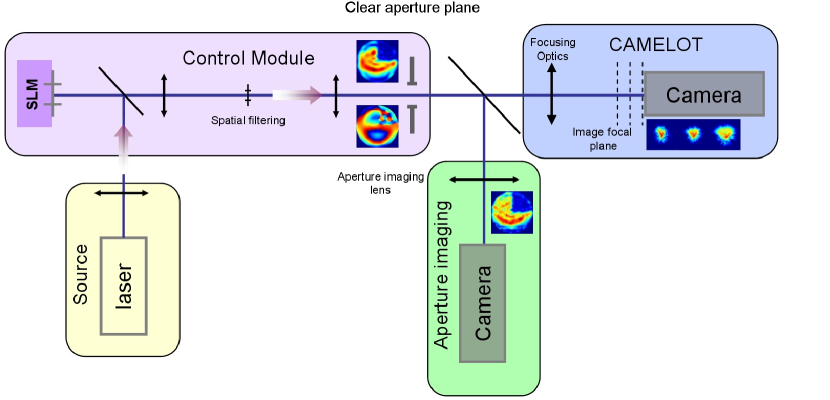
Figure 2: Experimental setup for camelot validation.

The spatial modulation of the laser beam (phase and modulus) is controlled by a field control module and conjugated with the clear aperture plane.

The beam going through the clear aperture crosses a beam splitter and is focused on the camelot camera of Fig. 1. The camera is used to record three near focal plane intensity distributions, which are given as inputs to camelot. The field estimated by the latter will be denoted $\psi_{c}=A_{C}e^{i\varphi_{C}}$ in the following. The beam reflected on the beam-splitter is used to record the intensity distribution $I_{M}$ with an image sensor conjugated with the aperture plane.

camelot’s estimation of the complex field is cross-validated in the two following ways: regarding field modulus, $A_{C}$ is compared with $A_{M}$, called measured modulus of the field hereafter, which is computed as the square-root of image $I_{M}$: $A_{M}=\sqrt{I_{M}}$.

Regarding phase, camelot’s estimate is compared to the result of a straightforward adaptation of a classical phase diversity algorithm [5] that will be referred to as conventional phase diversity. Phase diversity is now a well established technique: it has been used successfully for a number of applications [5], including very demanding ones such as extreme adaptive optics [6, 23], and its performance has been well characterized as a function of numerous factors, such as system miscalibration, image noise and artefacts, and algorithmic limitations [24]. In classical phase diversity, only the pupil phase is sought for, while the pupil transmittance is supposed to be known perfectly. This is probably the main limitation of this method, regardless of how the transmittance is known, whether by design or by measurement. In the case of a transmittance measurement, a dedicated imaging subsystem must be used, hence increasing the complexity of the setup. Misalignment issues (scaling, rotation of the pupil) have to be addressed due to the potential mismatch between the true pupil (which gives rise to the recorded image) and the pupil that is assumed in the image formation model. In this paper, for conventional phase diversity, the pupil transmittance is set to the measured modulus $A_{M}$ and the data used are two of the three near focal plane intensity distributions: the focal plane image and the first defocused image.

3.2 Control of the field

In this section, we present the modulation method used to control the field and how the result of the modulation is measured in the aperture plane.

The modulation of the complex amplitude is obtained using the field control method suggested by Bagnoud [25]: a phase modulator is followed by a focal plane filtering element.

The phase modulation is performed with a phase only SLM (Hamamatsu LCOS SLM x10-468-01) with 800x600 $20\,\text{\textmu{}m}$ pixels. The laser source is a $20\,\text{{mW}}$ continuous laser diode at $\lambda=650\,\text{nm}$ injected into a $4.6\,\text{\textmu{}m}$ core single-mode fiber. At the exit of the fiber, the beam is collimated, linearly polarized and then reflected on the SLM. The clear aperture diameter is $D=3\,\text{mm}$ on the surface of the SLM. It is conjugated with a unit magnification onto the clear aperture plane. The spatial modulation and filtering are designed to control 15$\times$15 resolution elements in the clear aperture i.e., 15 cycles per aperture. The effective result of the control in the clear aperture plane is called the true field. Its modulus is denoted $A_{T}$.

The spatial modulation and filtering have been modeled by means of an end-to-end simulation. The result of the simulation is denoted by $\psi_{S}$. Its modulus, denoted $A_{S}$, is presented on the left of Fig. 3. It shows smooth variations as can be typically observed on an intense pulsed laser [7]. It has been truncated in the upper right corner to simulate a strong vignetting effect. The phase of the field is presented on Fig. 4. It is dominated by a Zernike vertical coma ($Z_{7}$) of $11\leavevmode\nobreak\ \,\text{rad}$ Peak-to-Valley (PV), typical of a strong misalignment of a parabola for instance.

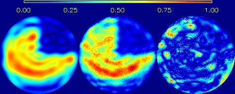
Figure 3: Left: modulus of the simulated field ($A_{S}$), center: measured modulus ($A_{M}$), right: $2.5\times|A_{M}-A_{S}|$.

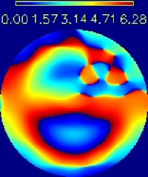
Figure 4: Phase of the simulated field.

The modulus of the true field is measured with the aperture plane imaging camera (see Fig.2). The image is recorded with a high spatial resolution (528 pixels in a diameter) and with a high SNR per pixel (60 in average). The result of the measurement,$A_{M}$, is presented at the center of Fig. 3.

In order to quantify the proximity of the simulated modulus $A_{S}$ with the measured one $A_{M}$, the following distance metric is defined:

$$\varepsilon^{2}_{MS}=\frac{\sum_{j=1}^{N_{0}}|{A_{M,j}-A_{S,j}}|^{2}}{\sum_{j=1}^{N_{0}}|{A_{S,j}}|^{2}}.$$ (14)

To enable their comparison, $A_{S}$ and $A_{M}$ have been normalized in flux ($\sum_{j=1}^{N_{0}}|{A_{S,j}}|^{2}=\sum_{j=1}^{N_{0}}|{A_{M,j}}|^{2}=1$).

The spatial distribution of the modulus of the difference between $A_{S}$ and $A_{M}$ is presented on the right of Fig. 3. It has been multiplied by a factor 2.5 to present a dynamic comparable to $A_{M}$.

The corresponding distance $\varepsilon^{2}_{MS}$ is found to be $\varepsilon^{2}_{MS}=0.044$, whereas in the case of a photon noise limited measurement simulations show that one should rather obtain $\varepsilon^{2}_{MS}=5\leavevmode\nobreak\ 10^{-5}$.

A preliminary Fourier-based analysis of the difference between $A_{S}$ and $A_{M}$ enables to identify a clear cut separation between spatial frequencies below the cut-off frequency of the spatial modulation (15 cycles per aperture) and higher spatial frequencies. Due to the spatial filtering by the control module, the low spatial frequencies part of the difference between $A_{S}$ and $A_{M}$ can be attributed mostly to model errors between the simple simulation performed to compute $A_{S}$ and the effective experimental setup of the control module. For instance in the simulation, the spatial filter is assumed to be centered on the optical axis, the SLM illumination is assumed to be perfectly homogeneous, and lenses and optical conjugations are supposed to be perfect. This part of $\varepsilon^{2}_{MS}$ is evaluated to $0.04$, that is more than $80\%$ of the total. The high frequencies part of $\varepsilon^{2}_{MS}$ comes from optical defects on relay optics and noise influence on $A_{M}$ measurement. It is evaluated to $4\leavevmode\nobreak\ 10^{-3}$. This gives insight on the measurement precision of $A_{M}$, which should thus be of the order of $4\leavevmode\nobreak\ 10^{-3}$.

3.3 camelot estimation

3.3.1 Practical implementation of phase diversity measurement

The intensity distributions in the different planes are recorded by translating the sensor along the optical axis around the focal plane. The amount of defocus must be large enough to provide significantly different intensity distributions so as to facilitate the estimation process. However, small translation distances are preferred for the sake of experimental easiness. For conventional phase diversity a defocus of $\lambda$ PV is often chosen as it maximizes the difference between the focal plane intensity distribution and the defocused image. Therefore, the amplitude of defocus between the position of each plane is fixed to $\lambda$ PV. Considering such a defocus, it appears that no less than three different measurement planes are required with camelot. The first image is located in the focal plane, the second one is at a distance corresponding to $\lambda$ of defocus PV, the third one at a distance of 2$\lambda$ PV from the focal plane. The relation between the PV optical path difference $\delta_{OPD}$ in the aperture plane and the corresponding translation distance between two successive planes $d_{kk+1}$ is:

$$d_{kk+1}=8(f/D)^{2}\delta_{OPD}.$$ (15)

For the experiment, the focusing optics focal length is $f=100\,\text{mm}$ and the aperture diameter is $D=3\,\text{mm}$. Consequently the translation distances are $d_{12}=d_{23}=5.78\,\text{mm}$ between the successive recording planes.

The intensity distributions are recorded with a Hamamatsu CMOS Camera (ORCA $R^{2}$). Its characteristics are the following: a pixel size and spacing $s_{pixel}=6.452\,\text{\textmu{}m}$, a readout noise standard deviation $\sigma_{ron}=6\leavevmode\nobreak\ e^{-}$ rms, a full well capacity of $18000\leavevmode\nobreak\ e^{-}$, and a $12$ bit digitizer.

As explained in Section 2.1, the sampling must fulfill the Shannon criterion. The focusing optics focal length and the aperture diameter combined with the pixel size lead to a theoretical Shannon oversampling factor $\lambda f/(2s_{pixel}D)=1.68$ for $\lambda=650\,\text{nm}$.

The total number of photo-electrons must be large enough to prevent the estimation from being noise limited. Simulations of the system that will be detailed in Section 4 demonstrate that $N_{phe}=5\times 10^{7}$ total photo-electrons are sufficient. Due to the limited full well capacity of the sensor, $p=10$ short exposures images are added to reach this number. For each image, background influence has been removed by a subtraction of an offset computed from the average of pixels located on the side of the images (hence not illuminated).

The noise covariance matrix $C_{k}$ is approximated by a diagonal matrix whose diagonal terms, $[C_{k}]_{jj}$, correspond to the sum of the variances of the photon noise, read out noise and quantization noise:

$$[C_{k}]_{jj}=[\sigma^{2}_{ph,k}]_{j}+p(\sigma^{2}_{ron}+q^{2}/12)$$ (16)

where $q$ is the quantization step. In practice, the readout noise variance map $\sigma^{2}_{ron}$ is calibrated beforehand and the photon noise variance $\sigma^{2}_{ph,k}$ is approximated from the image by: $[\hat{\sigma}^{2}_{ph,k}]_{j}=\max([\text{\boldmath$i$}_{k}]_{j},0)$ on pixel $j$ [26].

The three recorded near-focal intensity distributions are presented at the top of Fig. 5. The full size of one image is $N_{pix}=214\times 214$ pixels. For the figure, a region of interest of $140\times 140$ pixels, centered on the optical axis, is selected. From left to right the focal plane image, the first defocused image and the second one are displayed. The colorscale is logarithmic.

3.3.2 Results

The three focal plane images are now used in the camelot estimation. The minimization process is initiated with a homogeneous modulus field, a phase set to zero and differential tip/tilts also set to zero. The number of estimated points in the estimation plane is $N_{0}=64\times 64$. The current implementation of the algorithm is written in the IDL language.

A relevant measurement of the success of our inversion method is the quality of the match between the data $i_{k}$ and the model that can be computed from the estimated field through Eq (6). This latter map is presented on the middle row of Fig. 5. The moduli of the differences between the measurements and the direct model, that is to say estimation residuals, are displayed on the bottom row of the same figure. These residuals are below $1\%$ of the maximum of the measurements on the three planes.

The estimated shifts are $(-0.73,-0.56)$ and $(0.97,0.61)$ pixel for x and y directions for $P_{2}$ and $P_{3}$ respectively.

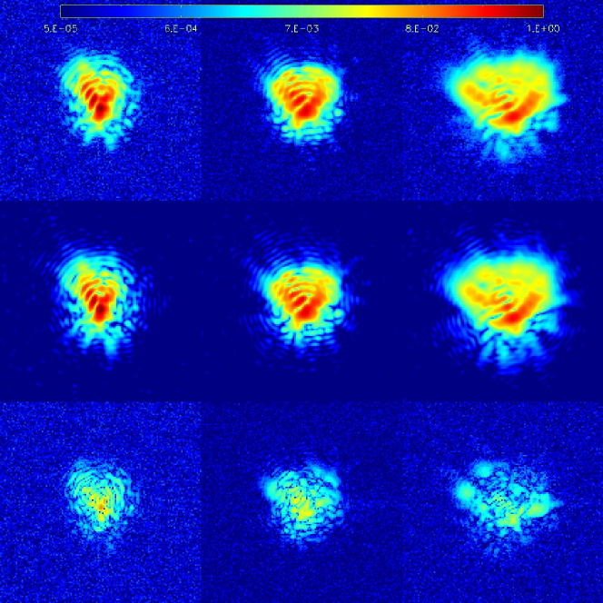
Figure 5: Left: focal plane images ($k=1$); center: first defocused images ($k=2$); right: second defocused image ($k=3$). Top: experimental images; middle: direct model result for $|{M_{k}\psi_{c}}|^{2}$; bottom: residuals, i.e., $|{\text{\boldmath$i_{k}$}-|{M_{k}\psi_{c}}|^{2}}|$. Logarithmic scale, $140\times 140$ pixels ROI centered on the optical axis.

The modulus of camelot’s estimated field, $A_{C}$, is presented on the left of Fig. 6. It has been normalized in flux to enable the comparison with the measured modulus $A_{M}$, shown in the center of the figure. For the comparison, $A_{M}$ has been sub-sampled and resized to $64$ pixels. The modulus of the difference between $A_{C}$ and $A_{M}$ is represented on the right. The main spatial structures of $A_{M}$ are well estimated by the method. The estimation residuals are below $20\%$ of the maximum of the measured modulus, even in the zones where the flux is low (top right corner). The distance between the two moduli is $\varepsilon^{2}_{A}=0.01$ only. This must be compared to the error between $A_{M}$ and $A_{S}$ reported in Section 3.2 which was found to be $0.044$. camelot thus delivers a modulus estimation that is several times closer to $A_{M}$ than $A_{S}$ is.

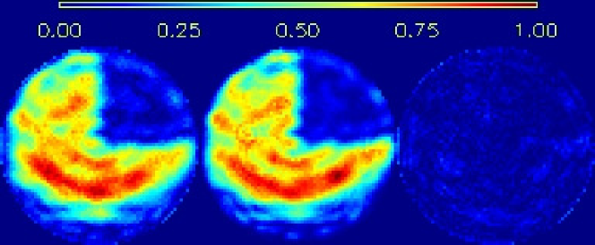
Figure 6: From left to right: $A_{c}$, $A_{M}$ and $|{A_{C}-A_{M}}|$.

We now compare the phase estimated by camelot to the result of the conventional phase diversity method described in Section 3.1. The comparison is presented on Fig. 7. The phase of $\psi_{C}$, $\varphi_{C}$, is presented on the left of the figure, the phase of the conventional phase diversity,$\varphi_{PD}$, is in the center of the figure, the modulus of their difference is presented on the right. For comparison of these phase maps, their differential piston has been set to 0. In the zones where the modulus is greater than $10\%$ of the maximum modulus of $\psi_{M}$, the maximum of the phase residuals is below $2\pi/10$  rad.

Additionally concerning conventional phase diversity, setting $A_{C}$ as the pupil transmittance instead of $A_{M}$ enables a better fit to the data with a 5% smaller criterion at convergence of the minimization, which is yet another indicator of the quality of the modulus $A_{C}$ estimated by camelot.

camelot and conventional phase diversity algorithms have about the same complexity. The former converges after less than 300 iterations and requires less than $10\min$ of computation, while the latter takes slightly more iterations and time. The main difference between the two methods lies in the modeling of the defocus between the measurement planes: in camelot it is performed by a Fresnel propagation, hence requiring two additional DFTs for each defocused plane. However, camelot appears here as fast as conventional phase diversity to achieve comparable results. The convergence time demonstrated here makes camelot suitable for the measurement and control of slowly varying aberrations such as those induced by thermal expansion of mechanical mounts for instance. The use of an appropriate regularization metric should contribute to speed up the computation. Recent work on real time conventional phase diversity demonstrated that few tens of Hertz are achievable with a dedicated (but commercial off-the-shelf) computing architecture [27]. According to the author of the latter reference, several hundreds of Hertz could even be achieved in a very near future, making phase diversity compatible with the requirements of the measurement and control of atmospheric turbulence effects. We believe that these conclusions can be generalized to camelot considering the similar convergence demonstrated here compared to conventional phase diversity and the the possibilities brought by Graphical Processing Units to speed up Fresnel propagation computations [28].

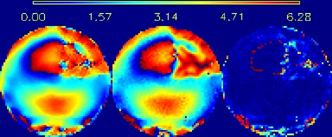
Figure 7: From left to right: $\varphi_{c}$, $\varphi_{PD}$ and $|{\varphi_{C}-\varphi_{PD}}|$.

4 Performance analysis by simulations

We now analyze the way these results compare with simulations. We simulate focal plane images from $\psi_{C}$ while taking into account the main disturbances that affect image formation: misalignments, photon and detector noises, limited full well capacity, quantization and miscalibration.

For the numerical simulation of the out-of-focus images, a random tip/tilt phase is added to the field before propagation to the imaging plane in order to simulate the effect of misalignment. The standard deviation of the latter corresponds to half a pixel in the focal plane.

Then two cases are considered. The first case, hereafter called perfect detector, assumes a detector with noise but an infinite well capacity and no quantization. Each image is first normalized by its mean number of photo-electrons $N_{phe,k}$, then for each pixel a Poisson occurrence is computed, and a Gaussian white noise occurrence with variance $\sigma_{ron}^{2}$ is then added to take into account the detector readout noise. The second case corresponds to a more realistic detector:

for a given value of the desired number of photo-electrons $N_{phe,k}$, the corresponding image is computed as the addition of as many “short-exposures” as needed in order to take into account the finite well capacity, and each of these short exposures is corrupted with photon noise, read-out noise and a 12 bit quantization noise. The same number of photo-electrons is attributed to each image : $N_{phe,k}=N_{phe}/N_{P}$ where $N_{phe}$ designates the total number of photo-electrons.

The simulated long exposure focal plane image is presented on the left of Fig. 8. This image is obtained for $N_{phe,1}=1.6\leavevmode\nobreak\ 10^{7}$ photo-electrons by adding $10$ short exposures. It can be visually compared with the experimental focal plane image recorded in comparable conditions (right): the similarity between the two images illustrates the relevance of the image simulation.

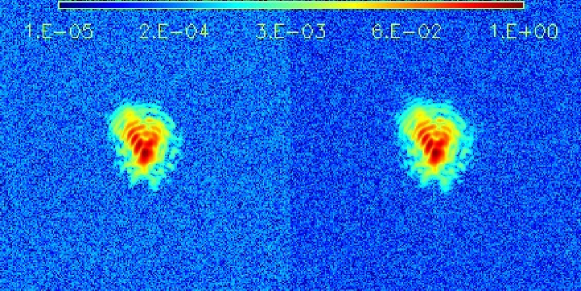
Figure 8: Focal plane images, left: simulation ($N_{phe,1}=1.6\leavevmode\nobreak\ 10^{7}$, $10$ short exposures), right: experiment.

The modulus estimation error $\varepsilon^{2}_{A}$ is plotted on Fig. 9 as a function of $N_{phe}$ for the two detector cases. Ten uncorrelated occurrences are averaged to compute $\varepsilon^{2}_{A}$. The result of the comparison of $A_{C}$ with $A_{M}$ obtained from the experiment is also reported on the figure (abscissa $N_{phe}=5\leavevmode\nobreak\ 10^{7}$ photo-electrons).

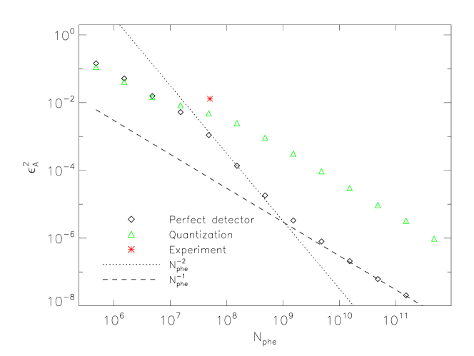
Figure 9: $\varepsilon^{2}_{A}$ as a function of average photo-electrons per pixel $N_{phe}$. Black diamonds ($\diamond$): perfect detector, green triangles ($\triangle$): finite well capacity and quantization, red asterisk ($\ast$): experiment result, dotted line: $N_{phe}^{-2}$, dashed line: $N_{phe}^{-1}$.

For the perfect detector case and $N_{phe}$ small compared to $5\leavevmode\nobreak\ 10^{8}$, $\varepsilon^{2}_{A}$ follows a $N_{phe}^{-2}$ power law. For greater values, the power law turns to $N_{phe}^{-1}$. This can be explained by the relative weights of the readout and the photon noise. For $N_{phe}\leq 5\leavevmode\nobreak\ 10^{8}$, the average flux on illuminated pixels, that can be approximated by $N_{phe}/(N_{P}\leavevmode\nobreak\ n_{i})$ where $n_{i}$ is the average number of illuminated pixels per image plane ($n_{i}\approx 100$), is smaller than the total readout noise contribution for one image plane, that is $N_{pix}^{2}\sigma_{ron}^{2}$. Thus, readout noise dominates. For $N_{phe}\geq 5\leavevmode\nobreak\ 10^{8}$, the photon noise contribution becomes predominant and the noise propagation of $\varepsilon^{2}_{A}$ follows a $N_{phe}^{-1}$ power law. It is confirmed here, as stated in Section 3.3, that $\varepsilon^{2}_{A}$ for the experiment is not limited by photon noise.

The analysis of $\varepsilon^{2}_{A}$ for the case with finite well capacity and quantization shows that it follows the perfect detector case up to about $N_{phe}=5\leavevmode\nobreak\ 10^{6}$ photo-electrons, then starts to follow a $N_{phe}^{-1}$ power law. $N_{phe}=5\leavevmode\nobreak\ 10^{6}$ corresponds to the flux necessary to saturate the well capacity of the sensor. Above this limit, images are added to emulate the summation of “short-exposures” images. Hence, the noise level in the measurements starts to depend on the number of summed images, that is to say on $N_{phe}$, with a $N_{phe}^{-1}$ power law.

The error level obtained from the comparison between the modulus measurement and camelot estimation ($\varepsilon^{2}_{MC}=0.013$) is comparable to the error level between camelot estimation and the true modulus in the case of the more realistic detector ($\varepsilon^{2}_{A}=5\leavevmode\nobreak\ 10^{-3}$): they differ approximately by a factor two. A significant part of this difference comes from the fact that the measured modulus $A_{M}$ too is imperfect i.e., is only an estimate of the true modulus $A_{T}$, due to experimental artefacts, notably differential optical defects that affect image formation on the aperture plane imaging setup and noise influence. This claim is also supported by the fact that the phase estimated by conventional phase diversity fits the measurements better when the pupil transmittance is set to the modulus estimated by camelot, $A_{C}$, instead of the measured modulus $A_{M}$. The Fourier-based analysis mentioned at the end of Section 3.2 delivers an estimate of the measurement precision of $A_{M}$ that is evaluated to $4\leavevmode\nobreak\ 10^{-3}$.

As a final remark, one can note that Fig. 9 can also be useful to evaluate not only the estimation error on the field modulus but the total error on the complex field itself. Indeed, we have calculated that this total error is on average simply twice the error on the modulus, or $2\varepsilon^{2}_{A}$. This can be particularly useful for designing a complex field measurement system based on camelot.

5 Conclusion

In this paper, we have demonstrated the applicability of phase diversity to the measurement of the phase and the amplitude of the field in view of laser beam control. The resolution of the inverse problem at hand has been tackled through a MAP/ML approach. An experimental setup has been designed and implemented to test the ability of the method to measure strongly perturbed fields representative of misaligned power lasers. The estimated field has been confronted to measured modulus using pupil plane imaging and to phases estimated with classical two-plane phase diversity (using the measured aperture plane modulus). It has been shown that the estimation accuracy is consistent with carefully designed numerical simulations of the experiment, which take into account several error sources such as noises and the influence of quantization. Noise propagation on the field estimation has been studied to underline the capabilities and limitations of the method in terms of photometry.

Several improvements to the method are currently considered. They include the estimation of a flux and of an offset per image, adding a regularization metric in the criterion to be optimized for the reconstruction of the complex field on a finer grid and speeding up the computations.

The work presented in this paper focuses on the case of a monochromatic beam. The application of camelot to the control of intense lasers with a wider spectrum, as it is the case for femtosecond lasers, must be investigated. Another limitation of the method lies in the computation time. For intense lasers, the correction frequency is small (typically a fraction of Hertz). camelot could therefore be used assuming a reasonable increase of computation speed. For real-time compensation of atmospheric turbulence in a an Adaptive Optics loop, a significant effort is requested to manage control frequencies above several hundred of Hertz. Application of the method to imaging systems with complicated pupil transmittance is also of interest.

The authors thank Baptiste Paul for fruitful discussions on classical phase diversity. This work has been performed in the framework of the Carnot project SCALPEL.