On the spectral stability of kinks in some $\mathcal{PT}$-symmetric variants of the classical Klein-Gordon Field Theories

Abstract.

In the present work we consider the introduction of $\mathcal{PT}$-symmetric terms in the context of classical Klein-Gordon field theories. We explore the implication of such terms on the spectral stability of coherent structures, namely kinks. We find that the conclusion critically depends on the location of the kink center relative to the center of the $\mathcal{PT}$-symmetric term. The main result is that if these two points coincide, the kink’s spectrum remains on the imaginary axis and the wave is spectrally stable. If the kink is centered on the “lossy side” of the medium, then it becomes stabilized. On the other hand, if it becomes centered on the “gain side” of the medium, then it is destabilized. The consequences of these two possibilities on the linearization (point and essential) spectrum are discussed in some detail.

1. Introduction

In the last 15 years, since its inception in the context of linear quantum mechanics [1], the study of systems with $\mathcal{PT}$ symmetry has gained tremendous momentum. While it was originally proposed as a modification/extension of quantum mechanics, its purview has gradually become substantially wider. This stemmed to a considerable degree from the realization that other areas such as optics might be ideally suited not only for its theoretical study [2, 3, 4], but also for its experimental realization [5, 6]. Hence, this effort has motivated a wide range of explorations focusing, among others, on the study of solitary waves and breathers in lattice and continuum systems [7, 8, 9, 10, 11, 12, 13, 14, 15], as well as on the complementary aspect of low-dimensional (oligomer or plaquette) settings [16, 17, 18, 19, 20].

Most of the above developments, however, have focused on the realm of Schrödinger type operators. However, other classes of Hamiltonian wave-bearing systems are of considerable interest in their own right, with a notable example being Klein-Gordon equations. This arises not only in the context of field theories (as e.g. in high energy/particle physics) [21, 22], but also in that of discrete (lattice nonlinear dynamical) systems with applications both to mechanics (e.g., arrays of coupled pendula; see e.g. for a recent example [23]) and to electrical systems (such as circuits consisting of e.g. capacitive and inductive elements [24]). It is interesting to note here that both at the mechanical level [25] and at the electrical one [26, 27] realizations of $\mathcal{PT}$ symmetry and its breaking have been recently implemented, while a Klein-Gordon setting has also been explored theoretically for so-called $\mathcal{PT}$ symmetric nonlinear metamaterials and the formation of gain-driven discrete breathers therein [28].

The aim of the present work is to formulate a prototypical field theoretic setting where gain and loss coexist in a balanced $\mathcal{PT}$ symmetric form in a Klein-Gordon model, around a central point which, without loss of generality, will be assumed to be at $0$. This addition to the standard Klein-Gordon model $u_{tt}=u_{xx}-V^{\prime}(u)$ will come into the form of a “dashpot” term $\gamma(x)u_{t}$. However, contrary to the usual setting where it has a negative definite prefactor incorporating dissipation (see e.g. the relevant local dissipation term in [23]), here this term will have a non-definite sign. In fact, to preserve the $\mathcal{PT}$ symmetry, $\gamma(x)$ will be anti-symmetric so that the transformation $(x,t)\mapsto(-x,-t)$ will leave the equation invariant. This suggests that there is a region where $\gamma(x)>0$, representing (without loss of generality) the “lossy” side of the medium, and a region where $\gamma(x)<0$, representing the “gain” side of the medium. For definiteness, in our numerical simulations we will assume that $\gamma(x)>0$ for $x<0$ (lossy side) and $\gamma(x)<0$ for $x>0$ (gain side).

Our principal aim is to explore the impact of this term on the stability properties of the coherent structures of this equation. Arguably, the most important among these are the ubiquitous kinks (heteroclinic connections in the ODE phase space which connect two distinct fixed points). Of substantial interest are also the relatively fragile breathers that exist in a time periodic exponentially localized form for some models (such as the sine-Gordon equation with $V(u)=1-\cos(u)$), but do not exist as such for others (such as the $\phi^{4}$ model with $V(u)=u^{2}-\frac{1}{2}u^{4}$). Here, given the fragility of the latter (breathers), we will focus solely on the former (kinks). Moreover, even for the kinks we will consider the simpler stationary problem, as the presence of $\gamma(x)$ and its breaking of translational invariance destroys the Lorentz invariance which produces traveling solutions out of static ones. Hence, it is not at all clear that traveling solutions exist in the model in the presence of the $\mathcal{PT}$ symmetric perturbation considered herein. Nevertheless, as the static problem $u_{xx}-V^{\prime}(u)=0$ is unaffected by our unusual antisymmetric dashpot, the steady state (kink) solutions persist in the proposed model and are, in fact, still available in explicit analytical form. For the sine-Gordon model they read $\phi(x)=4\arctan(\mathrm{e}^{(x-x_{0})})$, while for $\phi^{4}$, they are $\phi(x)=\tanh(x-x_{0})$. In each case, they can be centered at any $x_{0}$ along the real line. The fundamental question is therefore one of their spectral stability and it is that which we will try to resolve herein.

In particular, our mathematical analysis and numerical computations lead to the following conclusions:

1. if $x_{0}=0$, i.e., the kink is centered at the interface between gain and loss, then the spectrum is unaffected (with the exception of a possible shift of point spectrum imaginary eigenvalues which can move along the imaginary spectral axis) and the kink is spectrally stable;

2. if the kink is centered on the “lossy” side of the medium, the kink will be spectrally stable (excluding the possibility of an eigenvalue with a very small real part), with one of the formerly neutral eigenvalues (associated with translation) moving to the left half plane;

3. if the kink is centered on the “gain” side of the medium, it will be spectrally unstable with one of the formerly neutral eigenvalues (associated with translation) moving to the right half plane.

Our presentation is structured as follows. In section 2, we present the models and their solutions, and we set up the relevant spectral problem. In section 3 we prove a general result about the spectrum of a quadratic eigenvalue problem which can be considered to be a generalization of the problem associated with our two case examples. In section 4 we present some numerical computations which illustrate the theory. We conclude in section 5 with a brief discussion of our conclusions, and provide a possible list of future questions to be addressed.

2. Theoretical Setup and Principal Theorems

We consider the following basic PDE

(1) $$u_{tt}-u_{xx}+\epsilon\gamma(x)u_{t}+f(u)=0$$

Here $f(u)$ is a smooth nonlinear function that depends on the field $u$, and $\gamma(x)$ is a function accounting for the presence of gain/loss in the system. For $\epsilon=0$, and for some class of nonlinearities, there exist static kink solutions $\phi$, which will be the main object of consideration here. These will satisfy the following ODE

(2) $$-\phi_{xx}+f(\phi)=0.$$

As mentioned in the introduction, we will be particularly interested in the following examples:

• the sine-Gordon field theory, $f(u)=\sin(u)$, and the kink solution will be $\phi(x)=4\arctan(\mathrm{e}^{x})$

• the $\phi^{4}$ field theory, $f(u)=2(u^{3}-u)$, and the kink assumes the form $\phi(x)=\tanh(x)$.

The $\mathcal{PT}$ symmetry requires that the equation be invariant under the mapping $(x,t)\mapsto(-x,-t)$ (spatial reflection and time reversal). Clearly, the operator $\partial_{t}^{2}-\partial_{x}^{2}$ preserves the symmetry. In order for the operator $\gamma(x)\partial_{t}$ to also have this property, we need $\gamma(x)$ to be an odd function. This will be assumed throughout the rest of this paper.

Perturbing about the kink solution via the substitution $u(t,x)=\phi(x)+v(t,x)$, we obtain the linearized PDE

(3) $$v_{tt}-v_{xx}+\epsilon\gamma(x)v_{t}+f^{\prime}(\phi)v=0.$$

In our examples we have that

$$\lim_{x\to\pm\infty}f^{\prime}(\phi(x))=\sigma^{2}>0,$$

so that $W(x)\mathrel{\mathop{:}}=\sigma^{2}-f^{\prime}(\phi(x))$ is an effective potential which decays exponentially fast as $x\to\pm\infty$. We will henceforth assume that $\gamma(x)$ is also exponentially localized. Introducing the Schrödinger operator $\mathcal{H}$ with domain $H^{2}(\mathbf{R}^{1})$ in the form

$$\mathcal{H}=-\partial_{x}^{2}+f^{\prime}(\phi)=-\partial_{x}^{2}-W(x)+\sigma^{2},$$

we can rewrite the linearized problem as

$$v_{tt}+\epsilon\gamma(x)v_{t}+\mathcal{H}v=0.$$

Upon making the transformation

$$v(x,t)\mapsto v(x)\mathrm{e}^{\lambda t}$$

we have the spectral problem

$$\lambda^{2}v+\epsilon\lambda\gamma(x)v+\mathcal{H}v=0.$$

If the real part of the eigenvalue is positive, the wave will be spectrally unstable; otherwise, the wave is spectrally stable.

The Schrödinger operator $\mathcal{H}$ is self-adjoint, and by Weyl’s theorem its essential spectrum is given by $\sigma_{\mathrm{ess}}(\mathcal{H})=[\sigma^{2},+\infty)$. Moreover, since solutions to the existence problem (2) are invariant under spatial translation, it will be the case that the operator has a nontrivial kernel with $\mathcal{H}(\phi_{x})=0$. Alternatively, this fact follows immediately upon differentiating (2) with respect to $x$. In the next section we will stay away from the concrete $\mathcal{H}$ that arises in our application, and instead we will work with a general Schrödinger operator which satisfies relevant properties.

3. The quadratic eigenvalue problem

We have properly motivated our study of the following spectral problem:

(4) $$\mathcal{P}_{2}(\lambda)v\mathrel{\mathop{:}}=\lambda^{2}v+\epsilon\lambda\gamma(x)v+\mathcal{H}v=0.$$

Here $\mathcal{H}$ represents a self-adjoint Schrödinger operator on $H^{2}(\mathbb{R})$,

$$\mathcal{H}\mathrel{\mathop{:}}=-\partial_{x}^{2}-W(x)+\sigma^{2},\quad\sigma>0,$$

and $W(x)$ is a smooth function which decays exponentially fast,

$$|W(x)|\leq C\mathrm{e}^{-\alpha|x|},\quad\alpha>0.$$

We assume that $\gamma(x)$ is a smooth odd function which satisfies a similar exponential decay estimate as $W(x)$.

The exponential decay assumption on the potential $W(x)$ means that $\mathcal{H}$ is a relatively compact perturbation of the constant coefficient operator

$$\mathcal{H}_{\infty}\mathrel{\mathop{:}}=-\partial_{x}^{2}+\sigma^{2}$$

(see [29, Chapter 3.1] for the details). The essential spectrum of $\mathcal{H}$ is the spectrum of $\mathcal{H}_{\infty}$, and is given by

$$\sigma_{\mathrm{ess}}(\mathcal{H})=[\sigma^{2},+\infty).$$

Since $\mathcal{H}$ is a relatively compact perturbation of an operator of Fredholm index zero, the rest of the spectrum will be comprised of point eigenvalues, and each of these will have finite algebraic multiplicity. Moreover, basic Sturm-Liouville theory tells us that the point eigenvalues will be real and simple (e.g., see [29, Chapter 2.3]). Regarding the point spectrum of the Schrödinger operator $\mathcal{H}$, we make the following spectral assumptions:

Assumption 1.

The point spectrum of $\mathcal{H}$, say $\sigma_{0},\sigma_{1}^{2},\dots,\sigma_{n}^{2}$, is nonnegative and is ordered as

$$0=\sigma_{0}<\sigma_{1}^{2}<\cdots<\sigma_{n}^{2}<\sigma^{2}.$$

The associated eigenfunctions are labelled as $\psi_{0},\psi_{1},\dots,\psi_{n}$.

Quadratic eigenvalue problems are well-studied, and we refer to [30, 31, 32, 33] for some relevant results and references. One important result that we will use is that the quadratic problem (4) is equivalent to the linear eigenvalue problem

(5) $$\mathcal{L}\left(\begin{array}[]{c}v\\ w\end{array}\right)=\lambda\left(\begin{array}[]{c}v\\ w\end{array}\right),\quad\mathcal{L}\mathrel{\mathop{:}}=\left(\begin{array}[]{rc}0&1\\ -\mathcal{H}&-\epsilon\gamma(x)\end{array}\right).$$

As a consequence of this equivalence and the decay assumptions on $W(x)$ and $\gamma(x)$, the operator $\mathcal{L}-\lambda\bm{\mathit{I}}_{2}$ is Fredholm of index zero for all $\lambda$ which is not in the essential spectrum, $\sigma_{\mathrm{ess}}(\mathcal{L})$. The essential spectrum is found by considering the spectrum of the asymptotic operator

$$\mathcal{L}_{\infty}\mathrel{\mathop{:}}=\left(\begin{array}[]{cc}0&1\\ -\mathcal{H}_{\infty}&0\end{array}\right)$$

(the asymptotic operator is found by taking the limit $|x|\to\infty$ for $\mathcal{L}$). The essential spectrum is straightforward to compute, and we find it is purely imaginary,

$$\sigma_{\mathrm{ess}}(\mathcal{L})=(-\mathrm{i}\infty,-\mathrm{i}\sigma]\cup[\mathrm{i}\sigma,+\mathrm{i}\infty).$$

Regarding the point spectrum, $\sigma_{\mathrm{pt}}(\mathcal{L})$, because $\mathcal{L}$ is a relatively compact perturbation of $\mathcal{L}_{\infty}$ it will be the case that there are only a finite number of such eigenvalues, and each has finite algebraic multiplicity. Moreover, we have the symmetries as detailed below:

Lemma 1.

Suppose that $\epsilon\geq 0$. If $W(x)$ is even, then the point spectrum satisfies the Hamiltonian symmetry, $\{\pm\lambda,\pm\overline{\lambda}\}\subset\sigma_{\mathrm{pt}}(\mathcal{L})$. If $W(x)$ is not even, then all that can be said is the point spectrum is symmetric with respect to the real axis, $\{\lambda,\overline{\lambda}\}\subset\sigma_{\mathrm{pt}}(\mathcal{L})$.

Proof.

Setting $\bm{\mathit{v}}=(v\,\,w)^{\mathrm{T}}$, the fact that $\mathcal{L}$ has only real-valued entries implies that

$$\mathcal{L}\bm{\mathit{v}}=\lambda\bm{\mathit{v}}\quad\Rightarrow\quad\mathcal{L}\overline{\bm{\mathit{v}}}=\overline{\lambda}{\overline{\bm{\mathit{v}}}}.$$

Thus, the spectral symmetry with respect to the real axis is established. Now suppose that $W(x)$ is even. Setting $y=-x$ gives

$$\gamma(-y)=-\gamma(y),\quad W(-y)=W(y),$$

so that the quadratic problem becomes

$$\lambda^{2}z-\epsilon\lambda\gamma(y)z+\mathcal{H}z=0,\quad z(y)=v(-y).$$

The Schrödinger operator $\mathcal{H}$ is invariant under the spatial reflection. Upon setting $\gamma=-\lambda$ we recover the original eigenvalue problem, i.e.,

$$\mathcal{P}_{2}(\gamma)z=0.$$

Thus, under the assumption that $W(x)$ is even we see that if $\lambda$ is an eigenvalue with associated eigenfunction $v(x)$, then $-\lambda$ is an eigenvalue with associated eigenfunction $v(-x)$. ∎

Since the origin is an eigenvalue for $\mathcal{H}$ with eigenfunction $\psi_{0}$, it will be an eigenvalue for $\mathcal{L}$ with associated eigenfunction $(\psi_{0}\,\,0)^{\mathrm{T}}$. Moreover, since $\mathcal{H}$ is a Schrödinger operator, it is clear that the geometric multiplicity of the zero eigenvalue is one. Regarding the algebraic structure of this eigenvalue we have:

Lemma 2.

Suppose that $\epsilon>0$ is sufficiently small. The eigenvalue $\{0\}\subset\sigma_{\mathrm{pt}}(\mathcal{L})$ has algebraic multiplicity two if

$$\langle\gamma(x)\psi_{0},\psi_{0}\rangle=0,\quad\langle f,g\rangle\mathrel{\mathop{:}}=\int_{-\infty}^{+\infty}f(x)g(x)\,\mathrm{d}x.$$

Otherwise, it has algebraic multiplicity one.

Proof.

The generalized kernel is found by solving

$$\mathcal{L}\left(\begin{array}[]{c}v\\ w\end{array}\right)=\left(\begin{array}[]{c}\psi_{0}\\ 0\end{array}\right),$$

which with $w=\psi_{0}$ gives

$$\mathcal{H}v=-\epsilon\gamma(x)\psi_{0}.$$

By the Fredholm alternative this equation can be solved if and only if $\gamma(x)\psi_{0}\in\mathrm{Ker}(\mathcal{L})^{\perp}$, i.e.,

$$\langle\gamma(x)\psi_{0},\psi_{0}\rangle=0.$$

Supposing that the algebraic multiplicity is at least two, we will now show that the Jordan chain cannot be any longer. We start with

$$\mathcal{L}\left(\begin{array}[]{c}-\epsilon\mathcal{H}^{-1}[\gamma(x)\psi_{0}]\\ \psi_{0}\end{array}\right)=\left(\begin{array}[]{c}\psi_{0}\\ 0\end{array}\right).$$

If the chain is longer, then we can solve the linear system

$$\mathcal{L}\left(\begin{array}[]{c}v\\ w\end{array}\right)=\left(\begin{array}[]{c}-\epsilon\mathcal{H}^{-1}[\gamma(x)\psi_{0}]\\ \psi_{0}\end{array}\right),$$

which with $w=-\epsilon\mathcal{H}^{-1}[\gamma(x)\psi_{0}]$ gives

$$\mathcal{H}v=-\psi_{0}+\epsilon^{2}\gamma(x)\mathcal{H}^{-1}[\gamma(x)\psi_{0}].$$

Again invoking the Fredholm alternative, we see that this system has a solution if and only if

$$\begin{split}\langle\psi_{0},\psi_{0}\rangle&=\epsilon^{2}\langle\gamma(x)\mathcal{H}^{-1}[\gamma(x)\psi_{0}],\psi_{0}\rangle\\ &=\epsilon^{2}\langle\mathcal{H}^{-1}[\gamma(x)\psi_{0}],\gamma(x)\psi_{0}\rangle.\end{split}$$

By the spectral assumption on $\mathcal{H}$, i.e., all of the eigenvalues are nonnegative, as well as the assumption that $\langle\gamma(x)\psi_{0},\psi_{0}\rangle=0$, we know that

$$\langle\mathcal{H}^{-1}[\gamma(x)\psi_{0}],\gamma(x)\psi_{0}\rangle>0.$$

Thus, the equation can be guaranteed to not have a solution only if $\epsilon>0$ is not too large. ∎

Remark 1.

If $\epsilon=0$, then there is a Jordan chain of length two, and the generalized eigenfunction is given by $(0\,\,\psi_{0})^{\mathrm{T}}$.

Now that we understand the spectral structure at the origin, we consider the question of whether or not there can be eigenvalues which are arbitrarily large in magnitude with nonzero real part. Before doing so, let us consider the structure of the spectrum when $\epsilon=0$. The eigenvalue problem becomes

$$\mathcal{H}v=-\lambda^{2}v,$$

so that the eigenvalues for $\mathcal{L}$ are intimately related to those for $\mathcal{H}$. Indeed, as a consequence of the spectral assumption on $\mathcal{H}$, we see that there are precisely $n$ purely imaginary simple eigenvalues with positive imaginary part

$$\lambda_{j}=\mathrm{i}\sigma_{j},\quad j=1,\dots,n.$$

The spectral symmetry of Lemma 1 guarantees that there are $n$ purely imaginary eigenvalues with negative imaginary part. An associated eigenfunction for each eigenvalue with positive imaginary part is $(\psi_{j}\,\,\mathrm{i}\psi_{j})^{\mathrm{T}}$. Thus, arbitrarily large eigenvalues with nonzero real part for $\epsilon>0$ can exist only if they are somehow ejected from the essential spectrum.

Before continuing, we shall need the following technical result, which is sometimes called limited absorption principle. The limited absorption principle is a standard result, whose proof is based on appropriate estimates for the Jost solutions of the corresponding operator $L$. Its proof goes back to the fundamental work of [34], which was extended later by [35] and [36].

Lemma 3.

Consider the standard weighted $L^{2}$ space defined by the norm

$$\|f\|_{L^{2}_{\alpha}}\mathrel{\mathop{:}}=\left(\int_{-\infty}^{+\infty}|f(x)|^{2}(1+|x|^{2})^{\alpha}\,\mathrm{d}x\right)^{1/2}=:\|<x>^{\alpha}f\|_{L^{2}}.$$

For every $\delta>0$ there exists $C=C_{\delta,W}$ so that for all $\lambda\in\mathcal{C}$ with

$$\mathrm{dist}(\lambda,\sigma_{\mathrm{pt}}(\mathcal{H}))>\delta,$$

we have the estimate

(6) $$\|(\mathcal{H}-\lambda^{2})^{-1}\|_{L^{2}_{\frac{1}{2}+\delta}\to L^{2}_{-\frac{1}{2}-\delta}}\leq\frac{C}{|\lambda|}.$$

We are now ready to show that if $\epsilon>0$ is not too large, then there are no arbitrarily large eigenvalues.

Lemma 4.

There exists an $\epsilon_{0}>0$ and $M>0$ such that if $0\leq\epsilon<\epsilon_{0}$, then there exist no $\lambda\in\sigma_{\mathrm{pt}}(\mathcal{L})$ with nonzero real part such that $|\lambda|>M$.

Proof.

We prove by contradiction. Assume there is a sequence of point eigenvalues with nonzero real part $\lambda_{n}\to\infty$ corresponding to a sequence $\epsilon_{n}\to 0$. Let $\phi_{n}$ be a corresponding sequence of normalized eigenfunctions, $\|\phi_{n}\|=1$, so that $\mathcal{P}_{2}(\lambda_{n})\phi_{n}=0$, i.e.,

(7) $$(\mathcal{H}+\lambda_{n}^{2})\phi_{n}=-\epsilon_{n}\lambda_{n}\gamma(x)\phi_{n}.$$

Since $\lambda_{n}\to\infty$, we can apply the limited absorption principle in Lemma 3 to conclude that $\mathcal{H}+\lambda_{n}^{2}$ is invertible (at least in the sense of the weighted $L^{2}$ spaces as specified there), so

(8) $$\phi_{n}=-\epsilon_{n}\lambda_{n}(\mathcal{H}+\lambda_{n}^{2})^{-1}[\gamma(x)\phi_{n}].$$

Fixing $\delta=1/2$ (for example) and taking $L^{2}_{-1}$ norms in (8) yields

$$\begin{split}\|\phi_{n}\|_{L^{2}_{-1}}&\leq\frac{C}{|\lambda_{n}|}\epsilon_{n}|\lambda_{n}|\|\gamma(x)\psi_{n}\|_{L^{2}_{1}}\\ &\leq C\epsilon_{n}\left(\sup_{x}\left[<x>^{2}|\gamma(x)|\right]\right)\|\phi_{n}\|_{L^{2}_{-1}}.\end{split}$$

The last inequality leads to a contradiction, for $\epsilon_{n}\to 0$ as $n\to\infty$. ∎

We now consider the problem of whether or not any eigenvalues can be ejected from the essential spectrum when $\epsilon>0$. Alternatively, one can think of the following as a discussion on the resonances of a Schrödinger operator. Here we rely on the discussion of edge bifurcations for Schrödinger operators as presented in [29, Chapter 9.5]. Recalling the spectral symmetry about the real axis, assume that the imaginary part of $\lambda$ is positive. Upon setting

$$\mu^{2}\mathrel{\mathop{:}}=\sigma^{2}+\lambda^{2}\quad\Rightarrow\quad\lambda=\mathrm{i}\sqrt{\sigma^{2}-\mu^{2}},$$

the eigenvalue problem $\mathcal{P}_{2}(\lambda)v=0$ can be rewritten as

$$v_{xx}+W(x)v=\mu^{2}v+\mathrm{i}\epsilon\sqrt{\sigma^{2}-\mu^{2}}\,\gamma(x)v.$$

An important point here is that the branch point $\lambda=\mathrm{i}\sigma$ has been transformed to $\mu=0$. The transformation defines a two-sheeted Riemann surface in a neighborhood of the branch point. The physical sheet of this transformation, $\mu\in(-\pi/2,\pi/2)$, corresponds to eigenvalues for the original problem, while the resonance sheet, $\mu\in(\pi/2,3\pi/2)$, corresponds to resonance poles for the original problem. In a neighborhood of this branch point one can construct an analytic Evans function, $E(\mu)$, which has the property $E(\mu)=0$ if $\mu$ is an eigenvalue (physical sheet), or if $\mu$ is a resonance pole (resonance sheet).

First suppose that $\epsilon=0$. If $W(x)$ is a reflectionless potential, i.e., if $\mathcal{H}$ has a resonance at the edge of the essential spectrum, then there is a uniformly bounded but nondecaying solution, $\Psi$, at the branch point of $\mathcal{H}$,

(9) $$\mathcal{H}(\Psi)=\sigma^{2}\Psi,\quad\Psi(x)\to\begin{cases}\,\,1,\quad&x\to-\infty\\ \Psi_{+},\quad&x\to+\infty.\end{cases}$$

The Evans function notes the existence of this “eigenfunction” via $E(0)=0$ with $E^{\prime}(0)\neq 0$. If there is no resonance, then $E(0)\neq 0$. Since the Evans function is analytic, in a neighborhood of the branch point it will have no other possible zeros.

Now suppose that $\epsilon>0$ is small. The zero at the branch point will move to either the physical sheet or the resonance sheet, and in either case it will be of $\mathcal{O}(\epsilon)$. Denote this zero by $\mu_{1}\epsilon$, where $\mu_{1}=\mu_{1}(\epsilon)$. It is shown in [29, Theorem 9.5.1] that the expansion for this zero as applied to this problem is given by

(10) $$\mu_{1}=-\mathrm{i}\sigma\frac{\langle\gamma(x)\Psi,\Psi\rangle}{1+\Psi_{+}^{2}}+\mathcal{O}(\epsilon).$$

Here $\Psi$ is given in (9). Note that to leading order this zero is purely imaginary on the Riemann surface, and is consequently on the boundary between the physical sheet and the resonance sheet. If it moves onto the physical sheet, it will create an eigenvalue given by

$$\lambda=\mathrm{i}\sqrt{\sigma^{2}-\mu_{1}^{2}\epsilon^{2}}=\mathrm{i}\left(\sigma+\mathcal{O}(\epsilon^{2})\right).$$

The eigenvalue created by the edge bifurcation will be $\mathcal{O}(\epsilon^{2})$ close to the branch point. Because the leading order term in the expansion of $\mu_{1}(\epsilon)$ is purely imaginary, the $\mathcal{O}(\epsilon^{2})$ term in the expansion is purely real. Thus, if the eigenvalue has a nonzero real part it will necessarily be of $\mathcal{O}(\epsilon^{3})$. If the zero moves onto the resonance sheet, no eigenvalue is created. On the other hand, if the potential is not reflectionless, then no zeros will come out of the branch point. Finally, the Evans function analysis also shows that an eigenvalue can emerge from the essential spectrum only at the branch point.

Lemma 5.

Consider the spectral problem near the branch point $\lambda=\mathrm{i}\sigma$. If the potential $W(x)$ is reflectionless, then for $\epsilon>0$ small it is possible that there will be an eigenvalue which is $\mathcal{O}(\epsilon^{2})$ close to the branch point. The real part of the eigenvalue will be of $\mathcal{O}(\epsilon^{3})$. If the potential is not reflectionless, then no such eigenvalue can emerge. In either case there will be no other eigenvalues which have imaginary part greater than $\sigma+\mathcal{O}(\epsilon^{2})$.

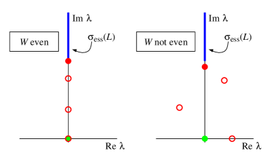
Figure 1. A cartoon which illustrates the possible spectrum for small $\epsilon$ when $W(x)$ is even (left panel) and $W(x)$ is not even (right panel). As a consequence of the spectral symmetry with respect to the real axis, only the upper-half of the complex plane is shown. The essential spectrum is given by a thick (blue) line, and the eigenvalue associated with a potential edge bifurcation is given by a filled (red) circle. The other nonzero eigenvalues are denoted by open circles. The double eigenvalue at the origin when $\epsilon=0$ is denoted by a filled circle. When $W(x)$ is even the eigenvalues remain purely imaginary, and the eigenvalue at the origin remains a double eigenvalue, whereas if $W(x)$ the eigenvalues will generically have nonzero real part, and the eigenvalue at the origin becomes simple. The potential simple eigenvalue arising from the edge bifurcation remains close to the edge of the essential spectrum.

We are now in position to give a full description of the spectrum for small $\epsilon>0$. The spectrum for $\epsilon=0$ is fully understood: it is purely imaginary, has a finite number of nonzero simple eigenvalues in the gap $(-\mathrm{i}\sigma,+\mathrm{i}\sigma)$, and has a geometrically simple eigenvalue at the origin with algebraic multiplicity two. For $\epsilon>0$ each of the nonzero eigenvalues will move a distance of $\mathcal{O}(\epsilon)$. Indeed, upon writing

$$\mathcal{L}=\left(\begin{array}[]{rc}0&1\\ -\mathcal{H}&0\end{array}\right)+\epsilon\left(\begin{array}[]{rc}0&0\\ 0&-\gamma(x)\end{array}\right),$$

and using the fact an eigenfunction associated to the eigenvalue $\mathrm{i}\sigma_{j}$ is $(\psi_{j}\,\,\mathrm{i}\psi_{j})^{\mathrm{T}}$, we see that after using standard perturbation theory (see [29, Chapter 6]) each of these eigenvalues will have the expansion

$$\lambda_{j}=\mathrm{i}\sigma_{j}-\epsilon\frac{\langle\gamma(x)\psi_{j},\psi_{j}\rangle}{2\langle\psi_{j},\psi_{j}\rangle}+\mathcal{O}(\epsilon^{2}).$$

In particular, if $\langle\gamma(x)\psi_{j},\psi_{j}\rangle\neq 0$, then the eigenvalue will move off the imaginary axis and have nonzero real part. As for the double eigenvalue at the origin, if $\langle\gamma(x)\psi_{0},\psi_{0}\rangle\neq 0$ one of the two eigenvalues will leave. The nonzero eigenvalue will be of $\mathcal{O}(\epsilon)$, and will have the expansion (again see [29, Chapter 6])

$$\lambda_{0}=-\epsilon\frac{\langle\gamma(x)\psi_{0},\psi_{0}\rangle}{\langle\psi_{j},\psi_{j}\rangle}+\mathcal{O}(\epsilon^{2}).$$

To leading order the nonzero eigenvalue will be purely real. The spectral symmetry with respect to the real axis guarantees that the nonzero eigenvalue is indeed real.

We are now ready to state our main result. The key control of the spectral structure is whether or not the potential $W(x)$ is an even function. The cartoon in Fig. 1 gives an illustration of the result.

Theorem 1.

Consider the quadratic spectral problem

$$\lambda^{2}v+\epsilon\lambda\gamma(x)v+\mathcal{H}v=0,$$

where $\mathcal{H}$ is the Schrödinger operator

$$\mathcal{H}=-\partial_{x}^{2}-W(x)+\sigma^{2}.$$

Assume that $W(x),\gamma(x)$ are exponentially localized, that $\gamma(x)$ is an odd function, and that $\epsilon>0$ is sufficiently small. Further suppose that $\mathcal{H}$ satisfies the spectral Assumption 1. If $W(x)$ is even, then the spectrum is purely imaginary, and the eigenvalue at the origin will have algebraic multiplicity two. If $W(x)$ is not even, the origin will be a simple eigenvalue, and there will be a purely real eigenvalue which has the expansion

(11) $$\lambda_{0}=-\epsilon\frac{\langle\gamma(x)\psi_{0},\psi_{0}\rangle}{\langle\psi_{0},\psi_{0}\rangle}+\mathcal{O}(\epsilon^{2}).$$

Moreover, in the upper-half plane there will be $n$ eigenvalues, each of which has the expansion

(12) $$\lambda_{j}=\mathrm{i}\sigma_{j}-\epsilon\frac{\langle\gamma(x)\psi_{j},\psi_{j}\rangle}{2\langle\psi_{j},\psi_{j}\rangle}+\mathcal{O}(\epsilon^{2}).$$

In particular, the real part will be $\mathcal{O}(\epsilon)$. Finally, there may be a simple eigenvalue near the branch point, but if so its real part will be $\mathcal{O}(\epsilon^{3})$.

Proof.

Suppose that $W(x)$ is even. For any $\epsilon\geq 0$ the spectrum satisfies the Hamiltonian symmetry $\{\pm\lambda,\pm\overline{\lambda}\}$. This symmetry first implies that if an eigenvalue is simple and purely imaginary for $\epsilon=0$, then it must remain so for $\epsilon>0$ sufficiently small. Indeed, it cannot leave the imaginary axis until it collides with another purely imaginary eigenvalue. If $W(x)$ is reflectionless, then it is possible for one eigenvalue to emerge from the essential spectrum through the edge bifurcation. The Hamiltonian spectral symmetry forces this eigenvalue to be purely imaginary for small $\epsilon$. Finally, the eigenvalue at the origin must remain a double eigenvalue. One eigenvalue must always remain at the origin due to $\mathcal{H}\psi_{0}=0$, and we know the other is purely real. But, the Hamiltonian symmetry implies that real eigenvalues come in pairs (symmetric about the imaginary axis). Since this scenario is precluded, the eigenvalue cannot leave.

On the other hand, if $W(x)$ is not even, then we have the perturbation expansions as proven before the statement of the theorem. ∎

Remark 2.

If $W(x)$ is even, then the eigenfunctions of the Schrödinger operator $\mathcal{H}$ are either even or odd. The assumption that the smallest eigenvalue of $\mathcal{H}$ is zero implies via Sturm-Liouville theory that the associated eigenfunction is even and nonzero. An eigenfunction associated with the eigenvalue $\sigma_{j}^{2}$ will be odd if $j$ is odd, and even if $j$ is even; moreover, it will have $j$ zeros. In any event, since $\gamma(x)$ is odd it will be the case that the first-order terms in the perturbation expansions will be zero; hence, if the nonzero eigenvalues move, they will do so at a rate of $\mathcal{O}(\epsilon^{2})$.

4. Numerical Results

We now turn to numerical considerations in order to identify the motion of the relevant eigenvalues and corroborate the predictions of Theorem 1. We first need to know the spectrum associated with the Schrödinger operator $\mathcal{H}$ for the sine-Gordon model and the $\phi^{4}$ model. We will henceforth assume that

$$\gamma(x)=-x\mathrm{e}^{-x^{2}/2},$$

so that $\gamma(x)>0$ for $x<0$ (lossy side), and $\gamma(x)<0$ for $x>0$ (gain side).

First consider the sine-Gordon model. Since

$$f^{\prime}(\phi)=\sin(\phi),\quad\phi(x)=4\arctan(\mathrm{e}^{x}),$$

we can write $\mathcal{H}$ as

$$\mathcal{H}=-\partial_{x}^{2}+\cos(\phi)=-\partial_{x}^{2}+(1-\cos(\phi))+1.$$

The branch point in the upper-half plane is $\lambda_{\mathrm{br}}=\mathrm{i}$. Since there is a bounded eigenfunction for $\mathcal{H}$ at the branch point $\sigma^{2}=1$,

$$\mathcal{H}(\Psi)=\Psi,\quad\Psi(x)=\tanh(x),$$

an Evans function analysis yields that the potential $W(x)=\cos(\phi)-1$ is reflectionless. Thus, it is possible for an eigenfunction to emerge from the branch point $\lambda_{\mathrm{br}}$. Other than the zero eigenvalue, there are no nonnegative eigenvalues. According to Theorem 1 the absence of point spectrum eigenvalues other than the double one at the origin suggests that to leading order this is the only eigenvalue that one needs to worry about under the effect of the $\mathcal{PT}$ symmetric term. The eigenvalue which arises from the origin will be real and of $\mathcal{O}(\epsilon)$, whereas the eigenvalue which potentially arises from the edge bifurcation will have a real part of $\mathcal{O}(\epsilon^{3})$.

Now consider the $\phi^{4}$ model. Since

$$f^{\prime}(\phi)=-2+6\phi^{2},\quad\phi(x)=\tanh(x),$$

we can write $\mathcal{H}$ as

$$\mathcal{H}=-\partial_{x}^{2}-2+6\phi^{2}=-\partial_{x}^{2}+6\mathop{\mathrm{missing}}{sech}\nolimits^{2}(x)+4.$$

Thus, $\sigma^{2}=4$, so the branch point in the upper-half plane is $\lambda_{\mathrm{br}}=\mathrm{i}2$. Regarding the point spectrum, the problem with $W(x)=-6\mathop{\mathrm{missing}}{sech}\nolimits^{2}(x)$ was considered in [29, Chapter 9.3.2]; see also [37]. Therein it was shown that this is a reflectionless potential, which implies that it is possible for an eigenvalue to emerge from the branch point $\lambda_{\mathrm{br}}$. Moreover, in addition to the zero eigenvalue there is one positive eigenvalue given by $\sigma^{2}=3$. According to Theorem 1 there are two eigenvalues of concern: the one near the origin, and the one near $\mathrm{i}\sqrt{3}$. Under the effect of the $\mathcal{PT}$ symmetric term there will again be a purely real eigenvalue of $\mathcal{O}(\epsilon)$, and unlike the sine-Gordon model there will also be an eigenvalue near $\mathrm{i}\sqrt{3}$ which has a real part of $\mathcal{O}(\epsilon)$. If an edge bifurcation occurs, the bifurcating eigenvalue will have a real part of $\mathcal{O}(\epsilon^{3})$.

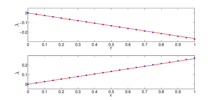
Figure 2. The shifting of the formerly neutral eigenvalue in the presence of a $\mathcal{PT}$ symmetric perturbation for the sine-Gordon model, as described in the text for a kink centered on the lossy side ($x_{0}=-2$, top) and one centered on the gain side ($x_{0}=2$, bottom). The dots denote numerical results for different values of $\epsilon$ (prefactor of the $\mathcal{PT}$ symmetric term), while the solid line yields the analytical prediction of Eq. (11) [see also the text]. Only for $\epsilon\approx 1$, does the numerical result start to weakly deviate from the explicit theoretical approximation.

The important point to note here is that each equation is invariant under spatial translation, so that a translate of a solution is also a solution. If we consider a solution which has been translated, then it the case that the eigenfunctions will be translated by the same amount. Translating the wave, i.e., moving its center, will act as a way to break symmetry. Moving the center will force the initially purely imaginary eigenvalues associated with the linearization about the centered wave (the wave balanced between the gain side and the lossy side) to gain a nontrivial real part.

Let us first consider the possible bifurcation from the origin for each model. For the sine-Gordon model we have

$$\phi(x-x_{0})=4\arctan(\mathrm{e}^{x-x_{0}})\quad\Rightarrow\quad\psi_{0}(x)=\mathop{\mathrm{missing}}{sech}\nolimits(x-x_{0}).$$

The associated potential $W(x)$ is even for $x_{0}=0$; otherwise, it is not. We know that the spectrum will be purely imaginary if $x_{0}=0$: the question is what happens for $x_{0}\neq 0$. A direct numerical calculation of the integrals associated with the perturbation expansion shows that for the eigenvalue bifurcating from the origin,

$$\lambda\sim\begin{cases}\,\,\,\,0.2675\epsilon,\quad&x_{0}=2\\ -0.2675\epsilon,\quad&x_{0}=-2\end{cases}$$

(see Fig. 2). In other words, if the underlying wave is centered on the gain side, then there will be a real positive eigenvalue and the wave will be unstable, whereas if the wave is centered on the loss side the bifurcating real eigenvalue will be negative. If it were the case that the potential eigenvalue emerging from the branch point $\lambda=\mathrm{i}$ also has nonpositive real part, then the wave would be spectrally stable. While we will not show the details here, a preliminary calculation suggests that if there is an eigenvalue which arises from an edge bifurcation, then the real part must be $\mathcal{O}(\epsilon^{3})$.

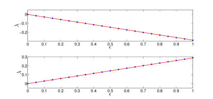
Figure 3. The same as the previous figure but now for the $\phi^{4}$ model.

For the $\phi^{4}$ model we have

$$\phi(x-x_{0})=\tanh(x-x_{0})\quad\Rightarrow\quad\psi_{0}(x)=\mathop{\mathrm{missing}}{sech}\nolimits^{2}(x-x_{0}).$$

The associated potential $W(x)$ is even for $x_{0}=0$; otherwise, it is not. We know that the spectrum will be purely imaginary if $x_{0}=0$: the question is what happens for $x_{0}\neq 0$. A direct numerical calculation of the integrals associated with the perturbation expansion shows that for the eigenvalue bifurcating from the origin,

$$\lambda\sim\begin{cases}\,\,\,\,\,0.2876\epsilon,\quad&x_{0}=+2\\ -0.2876\epsilon,\quad&x_{0}=-2\end{cases}$$

(see Fig. 3). Again, if the underlying wave is centered on the gain side, then there will be a real positive eigenvalue and the wave will be unstable, whereas if the wave is centered on the loss side the bifurcating real eigenvalue will be negative. There is the additional eigenvalue which starts at $\lambda=\mathrm{i}\sqrt{3}$. Since

$$\psi_{1}(x)=\tanh(x)\mathop{\mathrm{missing}}{sech}\nolimits(x)$$

(see [37]), a numerical calculation of the integrals gives

$$\lambda\sim\mathrm{i}\sqrt{3}+\begin{cases}\,\,\,\,\,0.1137\epsilon,\quad&x_{0}=+2\\ -0.1137\epsilon,\quad&x_{0}=-2\end{cases}$$

(see Fig. 4 for the case of $x_{0}=-2$, and Fig. 5 for the case of $x_{0}=2$). As is the case with the eigenvalue bifurcating from the origin, if the wave is centered on the gain side, the real part of the eigenvalue will be positive, whereas if the wave is centered on the lossy side, the real part will be negative. If it were the case that the potential eigenvalue emerging from the branch point $\lambda=\mathrm{i}2$ also has nonpositive real part, then the wave would be spectrally stable. While we will not show the details here, a preliminary calculation again suggests that if there is an eigenvalue which arises from an edge bifurcation, then the real part must be $\mathcal{O}(\epsilon^{3})$.

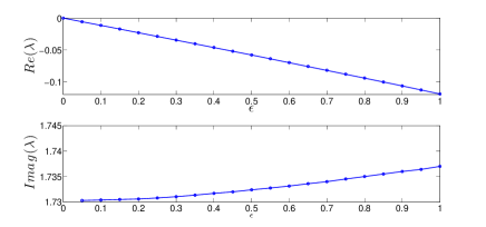
Figure 4. The figure shows the dependence of the real (top) and imaginary (bottom) part of the eigenvalue originally (i.e., for $\epsilon=0$) located at $\lambda^{2}=-3$ for the $\phi^{4}$ model. For the kink centered at $x_{0}=-2$, the perturbation knocks this pair off of the imaginary axis and into a complex pair in the left half plane, implying spectral stability.

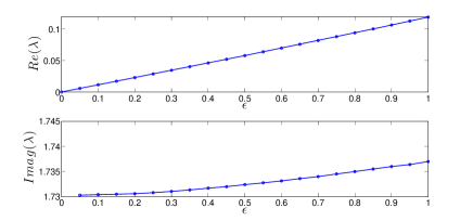
Figure 5. The same as the previous figure but now for the case of $x_{0}=2$, leading to (additional) instability due to the bifurcation of the relevant eigenvalue to the right half plane.

5. Conclusions and Future Challenges

In this work, we have introduced a $\mathcal{PT}$-symmetric variant of the widely relevant (in mechanical, electrical and other physical systems –as e.g. in particle physics–) Klein-Gordon field theory. We have done so by incorporating an anti-symmetric dashpot term featuring gain on one side of the domain and loss symmetrically on the other side. While such $\mathcal{PT}$-symmetric Klein-Gordon settings are starting to be analyzed even experimentally at the discrete level (especially in the case of few nodes), the case of the continuum limit is virtually unexplored. We have seen that for such systems, the stationary kink states of the model persist; however, their spectral stability is dramatically affected. If the kinks of interest are centered at the exact interface between the gain and loss, then they preserve their spectral stability, a feature that our Theorem 1 allows us to establish rigorously. If they are centered on the lossy side, they become further stabilized with parts of the point spectrum moving to the left half plane (either on the real axis or as complex eigenvalue pairs). In this case, if there is a spectral instability, it is weak, for the real part of the unstable eigenvalue will be $\mathcal{O}(\epsilon^{3})$. On the other hand, by means of the symmetries of the model, it is evident that when they are centered on the gain side of the medium, then the relevant eigenvalues bifurcate to the right half plane, giving rise to instability.

While the above lay some of the foundations of the subject of $\mathcal{PT}$-symmetric Klein-Gordon field theories, there are numerous questions that remain open both as regards the existence and in connection to the stability properties of coherent structures in such models. A feature that we did not touch upon, which our preliminary observations suggest that it is even numerically quite technically challenging is the fate of the resonance in the case of $x_{0}\neq 0$. Understanding whether this edge bifurcation from the continuous spectrum may contribute to an instability in such a setting would be a topic of theoretical and numerical interest in its own right. In addition, it would be interesting to develop an instability index theory for such quadratic polynomials in which the linear coefficient is not definite. As was seen in [38] in the case of quadratic matrix polynomials, if the linear coefficient is definite, then the total number of eigenvalues with positive real part is bounded above by the total number of negative eigenvalues for the Schrödinger operator $\mathcal{H}$. Unfortunately, the proof of this result heavily depended upon the definiteness of the linear term, and consequently it is not clear as to how it can be extended to the problem considered in this paper.

As noted earlier there are states which are genuinely time-dependent in Klein-Gordon models, and these states include the traveling kinks and the breathers. While one may be inclined to doubt the existence of genuinely traveling kinks given the spatial inhomogeneity imposed by the gain-loss profile, it would be interesting to explore the dynamics of such waves. For the breathers it is unclear whether the $\mathcal{PT}$-symmetric extension will preserve their structure (and if so, under which conditions this may occur). These questions are currently under consideration and will be reported in future publications.

References

- [1] C. M. BENDER, “Making Sense of Non-Hermitian Hamiltonians”, Rep. Prog. Phys. 70 (2007) 947–1018.
- [2] Z. H. MUSSLIMANI, K. G. MAKRIS, R. EL-GANAINY, and D. N. CHRISTODOULIDES, Optical Solitons in PT Periodic Potentials, Phys. Rev. Lett. 100 (2008) 030402 (4 pages).
- [3] H. RAMEZANI, T. KOTTOS, R. EL-GANAINY, and D.N. CHRISTODOULIDES, “Unidirectional nonlinear PT-symmetric optical structures”, Phys. Rev. A 82 (2010), 043803 (6 pages).
- [4] A. RUSCHHAUPT, F. DELGADO, and J.G. MUGA, “Physical realization of PT-symmetric potential scattering in a planar slab waveguide”, J. Phys. A: Math. Gen. 38 (2005) L171–L176.
- [5] A. GUO, G.J. SALAMO, D. DUCHESNE, R. MORANDOTTI, M. VOLATIER-RAVAT, V. AIMEZ, G. A. SIVILOGLOU, and D. N. CHRISTODOULIDES, “Observation of PT - symmetry breaking in complex optical potentials”, Phys. Rev. Lett. 103, 093902 (2009).
- [6] C.E. RÜTER, K.G. MAKRIS, R. EL-GANAINY, D.N. CHRISTODOULIDES, M. SEGEV, and D. KIP, “Observation of parity-time symmetry in optics”, Nature Physics 6 (2010) 192–195.
- [7] F.Kh. ABDULLAEV, Y.V. KARTASHOV, V.V. KONOTOP, and D.A. ZEZYULIN, “Solitons in PT-symmetric nonlinear lattices”, Phys. Rev. A 83 (2011), 041805(R) (4 pages).
- [8] N. V. ALEXEEVA, I. V. BARASHENKOV, A.A. SUKHORUKOV, and YU.S. KIVSHAR, “Optical solitons in PT-symmetric nonlinear couplers with gain and loss”, Phys. Rev. A 85 (2012), 063837 (13 pages)
- [9] I.V. BARASHENKOV, S.V. SUCHKOV, A.A. SUKHORUKOV, S.V. DMITRIEV and YU.S. KIVSHAR, “Breathers in PT-symmetric optical couplers”, Phys. Rev. A 86 (2012) 053809 (12 pages)
- [10] R. DRIBEN and B.A. MALOMED, “Stability of solitons in parity-time-symmetric couplers”, Opt. Lett. 36 (2011), 4323–4325.
- [11] R. DRIBEN and B.A. MALOMED, “Stabilization of solitons in PT models with supersymmetry by periodic management ”, EPL 96 (2011), 51001 (6 pages).
- [12] S. NIXON, L. GE, and J. YANG, “Stability analysis for solitons in PT-symmetric optical lattices”, Phys. Rev. A 85 (2012), 023822 (10 pages).
- [13] S.V. DMITRIEV, A.A. SUKHORUKOV, and YU.S. KIVSHAR, “Binary parity-time-symmetric nonlinear lattices with balanced gain and loss”, Opt. Lett. 35 (2010), 2976–2978.
- [14] V.V. KONOTOP, D.E. PELINOVSKY, and D.A. ZEZYULIN, “Discrete solitons in PT-symmetric lattices”, EPL 100 (2012), 56006 (6 pages).
- [15] A.A. SUKHORUKOV, S.V. DMITRIEV, S.V. SUCHKOV, and YU.S. KIVSHAR, “Nonlocality in PT-symmetric waveguide arrays with gain and loss” Opt. Lett. 37 (2012) 2148-2150.
- [16] K. LI and P.G. KEVREKIDIS, “PT-symmetric oligomers: analytical solutions, linear stability, and nonlinear dynamics”, Phys. Rev. E 83 (2011), 066608 (7 pages).
- [17] K. LI, P.G. KEVREKIDIS, B.A. MALOMED, and U. GÜNTHER, “Nonlinear PT-symmetric plaquette”, J. Phys. A Math. Theor. 45 (2012) 444021 (23 pages)
- [18] S.V. SUCHKOV, B.A. MALOMED, S.V. DMITRIEV and YU.S. KIVSHAR, “Solitons in a chain of parity-time-invariant dimers”, Phys. Rev. E 84 (2011), 046609.
- [19] A.A. SUKHORUKOV, Z. XU, and YU.S. KIVSHAR, “Nonlinear suppression of time reversals in PT-symmetric optical couplers” Phys. Rev. A 82 (2010), 043818 (5 pages).
- [20] D.A. ZEZYULIN and V.V. KONOTOP, “Nonlinear modes in finite-dimensional PT-symmetric systems” Phys. Rev. Lett. 108 (2012), 213906 (5 pages).
- [21] T. DAUXOIS and M. PEYRARD, Physics of Solitons, Cambridge University Press, (Cambridge, 2006).
- [22] R. K. DODD, J. C. EILBECK, J. D. GIBBON, and H.C. MORRIS, Solitons and Nonlinear Wave Equations Academic Press (New York, 1983).
- [23] J. CUEVAS, L. Q. ENGLISH, P.G. KEVREKIDIS, and M. ANDERSON, “Discrete Breathers in a Forced-Damped Array of Coupled Pendula: Modeling, Computation, and Experiment”, Phys. Rev. Lett. 102, 224101 (2009).
- [24] M. REMOISSENET, Waves Called Solitons, Springer-Verlag (Berlin, 1999).
- [25] C.M. BENDER, B.J. BERNTSON, D. PARKER and E. SAMUEL, “Observation of PT-phase transition in a simple mechanical system”, Am. J. Phys. 81, 173 (2013).
- [26] J. SCHINDLER, A. LI, M. C. ZHENG, F. M. ELLIS, and T. KOTTOS, “Experimental study of active LRC circuits with symmetries”, Phys. Rev. A 84, 040101 (2011).
- [27] H. RAMEZANI, J. SCHINDLER, F. M. ELLIS, U. GÜNTHER, and T. KOTTOS, “Bypassing the bandwidth theorem with symmetry”, Phys. Rev. A 85, 062122 (2012).
- [28] N. LAZARIDES and G. P. TSIRONIS, “Gain-Driven Discrete Breathers in PT-Symmetric Nonlinear Metamaterials” Phys. Rev. Lett. 110, 053901 (2013).
- [29] T. KAPITULA and K. PROMISLOW, “Spectral and Dynamical Stability of Nonlinear Waves”, Springer-Verlag (2013).
- [30] J. BRONSKI, M. JOHNSON, and T. KAPITULA, “An instability index theory for quadratic pencils and applications”, Comm. Math. Phys. (2014), to appear.
- [31] M. STANISLAVOVA, A. STEFANOV, Linear stability analysis for traveling waves of second order in time PDE’s, Nonlinearity 25, (2012) p. 2625–2654.
- [32] M. STANISLAVOVA, A. STEFANOV, Spectral stability analysis for special solutions of second order in time PDE’s: the higher dimensional case, Physica D, 262 (2013), p. 1–13.
- [33] M. CHUGUNOVA and D. PELINOVSKY, “On quadratic eigenvalue problems arising in stability of discrete vortices”, Lin. Alg. Appl. 431 (2009) 962–973.
- [34] S. AGMON, “Spectral properties of Schrödinger operators and scattering theory”, Ann. Scuola Norm. Sup. Pisa Cl. Sci. (4) 2 (1975), no. 2, 151–218.
- [35] A. JENSEN, T. KATO, “Spectral properties of Schrödinger operators and time-decay of the wave functions” Duke Math. J. 46 (1979), no. 3, 583–611.
- [36] P. DEIFT, E. TRUBOWITZ, “Inverse scattering on the line” Comm. Pure Appl. Math. 32 (1979), no. 2, 121–251.
- [37] T. SUGIYAMA, “Kink-Antikink collisions in the two-dimensional model”, Prog. Theor. Phys. 61, 1550 (1979).
- [38] T. KAPITULA, E. HIBMA, H.-P. KIM, and J. TIMKOVICH, “Instability indices for matrix polynomials”, Linear Algebra Appl. 439(11), 3412-3434 (2013). (2013)