Multi-reference symmetry-projected variational approximation for the ground state of the doped one-dimensional Hubbard model

Abstract

A multi-reference configuration mixing scheme is used to describe the ground state, characterized by well defined spin and space group symmetry quantum numbers as well as doping fractions $N_{e}/N_{sites}$, of one dimensional Hubbard lattices with nearest-neighbor hopping and periodic boundary conditions. Within this scheme, each ground state is expanded in a given number of nonorthogonal and variationally determined symmetry-projected configurations. The results obtained for the ground state and correlation energies of half-filled and doped lattices with 30, 34 and 50 sites, compare well with the exact Lieb-Wu solutions as well as with the ones obtained with other state-of-the-art approximations. The structure of the intrinsic symmetry-broken determinants resulting from the variational procedure is interpreted in terms of solitons whose translational and breathing motions can be regarded as basic units of quantum fluctuations. It is also shown that in the case of doped 1D lattices, a part of such fluctuations can also be interpreted in terms of polarons. In addition to momentum distributions, both spin-spin and density-density correlation functions are studied as functions of doping. The spectral functions and density of states, computed with an ansatz whose quality can be well-controlled by the number of symmetry-projected configurations used to approximate the $N_{e}\pm 1$ electron systems, display features beyond a simple quasiparticle distribution, as well as spin-charge separation trends.

I Introduction.

Disentangling the effects of electron-electron interactions in the ground and excited states of low-dimensional systems has become an exciting challenge in contemporary condensed matter physics. Dagotto-review ; Dagotto-Rev-Mod-Physics-2013 In particular, the discovery of high-Tc superconductivity in the cuprates HTCSC-1 has acted as a driving force to develop theoretical models able to account for the most relevant correlations in many-electron systems in the simplest possible way. Within this context, the repulsive Hubbard model Hubbard-model_def1 has been widely studied for several reasons including that it represents a prototype for the Mott transition between a metal and an antiferromagnetic insulator Vollhardt and the suggestion Anderson-1 that it contains the basic physics associated with high-Tc superconductivity. The phenomenon of colossal magnetic resistance Science-Dagotto has also attracted considerable attention. On the other hand, the study of the high-Tc iron-based superconductors sup-Fe ; Stewart-Review has become a very active research area. Su-Fe-Dagotto Here, calculations in terms of multi-orbital Hubbard-like models have already provided valuable insight into the interplay between doping and the strength of the electronic correlations in these exotic superconductors. Dagotto-Rev-Mod-Physics-2013 Hubbard models represent valuable tools to study cold fermionic atoms in optical lattices optical-1 as well as the properties of graphene. CastroNeto-review It has also become clear that their strong coupling limits, i.e., the Heisenberg models, text-Hubbard-1D can be quite useful to study low-dimensional magnets whose properties might be relevant for real materials found in nature and/or synthesized by means of crystal growing. Mikeska

The previous examples already show the central role of Hubbard-like lattice models and their strong coupling versions to obtain insight into the properties associated with the emergent complexity in many-electron problems. Precisely, it is this complexity that requires the use of different approximations to describe low-dimensional systems. Among the available theoretical tools we have, for example, exact diagonalizations for small lattices Dagotto-review ; Lanczos-Fano while for the larger ones, we can resort to quantum Monte Carlo, Nightingale ; Raedt-MC variational Monte Carlo, Neuscamman-2012 coupled cluster, Bishop-1 ; Bishop-2 variational reduced-density-matrix var-red-den-mat and density matrix renormalization group DMRG-White ; Dukelsky-Pittel-RPP ; Scholl-RMP methods, as well as approximations based on matrix product and tensor network states. Scholl-AP ; GChan ; TNPS-1 ; TNPS-2 Both frequency-dependent and frequency-independent embedding approaches Zgid ; DMFT-1 ; maier2005 ; stanescu2006 ; moukouri2001 ; huscroft2001 ; aryanpour2003 ; DVP-2 ; Knizia-Chan ; Irek-DMET are also actively pursued.

Table 1: Ground state energies for half-filled and doped lattices with $N_{sites}$=30 sites and $N_{e}$=14, 18, 22, 26, 30 electrons predicted with the FED scheme ($n$=60 GHF transformations for $U$=2$t$, 4$t$ and $n$=150 for $U$=8$t$) are compared with exact values. Results obtained with the FED^∗ [$n$=25 GHF transformations] (Ref. 51), and ResHF [$n$=30 UHF transformations] (Ref. 41) approximations as well as the energies corresponding to the RHF and other HF solutions are also included in the table. The ratio of correlation energies $\kappa$, is computed according to Eq.(9).

$U$					$N_{e}$=30	$\kappa(\%)$		$N_{e}$=26	$\kappa(\%)$			$N_{e}$=22	$\kappa(\%)$		$N_{e}$=18	$\kappa(\%)$		$N_{e}$=14	$\kappa(\%)$
2$t$			RHF		-23.2671			-26.1642				-26.8921			-25.5587			-22.3390
			HF		-23.4792	10.02		-26.1642	0			-26.8921	0		-25.5587	0		-22.3390	0
			FED		-25.3800	99.83		-28.0201	99.72			-28.4391	99.68		-26.7816	99.69		-23.2365	99.74
			FED∗		-25.3730	99.50		-	-			-	-		-	-		-
			ResHF		-25.3436	98.11		-27.9979	98.52			-28.4268	98.88		-	-		-	-
			Exact		-25.3835			-28.0253				-28.4441			-26.7854			-23.2388
4$t$			RHF		-8.2671			-14.8975				-18.8254			-20.1587			-19.0723
			HF		-14.0732	64.75		-17.3756	34.96			-20.1328	23.42		-21.1011	22.45		-19.8855	27.84
			FED		-17.2081	99.71		-21.9193	99.04			-24.3497	99.03		-24.3222	99.19		-21.9824	99.63
			FED∗		-17.1789	99.39		-	-			-	-		-	-		-
			ReSHF		-17.0542	98.00		-21.5720	94.15			-24.1582	95.56		-	-		-	-
			Exact		-17.2335			-21.9868				-24.4057			-24.3561			-21.9932
8$t$			RHF		21.7329			7.6358				-2.6921			-9.3587			-12.5390
			HF		-7.8329	93.65		-11.2049	79.45			-14.9299	69.32		-18.1922	70.12		-19.0005	77.96
			FED		-9.8260	99.95		-15.8927	99.22			-20.1711	99.01		-21.8777	99.38		-20.8062	99.75
			FED∗		-9.7612	99.75		-	-			-	-		-	-		-
			ResHF		-9.5378	98.46		-15.4059	97.17			-19.5552	95.52		-	-		-	-
			Exact		-9.8387			-16.0761				-20.3462			-21.9555			-20.8271

The exact Bethe ansatz solution of the one-dimensional (1D) Hubbard Hamiltonian is well known, LIEB ; BETHE which is not the case for the two-dimensional (2D) model. On the other hand, in spite of the considerable progress already made, the exact 1D wave functions still remain difficult to handle in practice when computing several physical properties. text-Hubbard-1D It has also remained difficult to obtain an intuitive physical picture of the basic units of quantum fluctuations Tomita-3 ; Tomita-1 ; Tomita-2 ; Tomita-2011PRB using the Lieb-Wu solutions LIEB and/or within the theoretical frameworks already mentioned above. This task is further complicated by the fact that quantum fluctuations can exhibit unconventional features in low-dimensional systems. A typical example, is the spin-charge separation in the strong coupling regime of the 1D Hubbard model. text-Hubbard-1D ; Ogata-Shiba ; Voit Angle-resolved photoemission spectroscopy results also reveal a complex pattern of spin-charge coupling/decoupling both in 1D and 2D systems Kim ; KMShen in the weak and intermediate-to-strong interaction regimes.

Therefore, it is highly desirable to explore the performance of alternative wave function based approaches that, on the one hand, could complement existing state-of-the-art theoretical tools and, on the other hand, lead us to compact states whose (intrinsic) structures are simple enough to be interpreted in terms of basic units of quantum fluctuations in half-filled and doped lattices. Within this context, the 1D Hubbard model represents a challenging testing ground since both its exact solution and highly accurate density matrix renormalization group results are available. The last years have seen some progress in this direction within the framework of the single-reference (SR) and multi-reference (MR) symmetry-projected approximations Tomita-1 ; Tomita-2 ; Tomita-2011PRB ; Carlos-Hubbard-1D ; Rayner-2D-Hubbard-PRB-2012 ; non-unitary-paper-Carlos ; rayner-Hubbard-1D-FED2013 which are routinely used in nuclear structure physics. rs ; Carlo-review ; rayner-GCM-paper ; rayner-GCM-parity Note that in quantum chemistry the names single-component and multi-component have been adopted Carlos-Rayner-Gustavo-VAMPIR-molecules ; Carlos-Rayner-Gustavo-FED-molecules instead of single-reference and multi-reference , respectively.

Recently, a hierarchy of symmetry-projected variational approaches Carlo-review has been applied to describe both the ground and excited states of the 1D and 2D Hubbard models. Carlos-Hubbard-1D ; Rayner-2D-Hubbard-PRB-2012 ; non-unitary-paper-Carlos ; rayner-Hubbard-1D-FED2013 In its simplest (i.e., SR) form, the symmetry-projected variation-after-projection (VAP) method Carlos-Hubbard-1D resorts to a Hartree-Fock-type rs (HF) trial state $|{\cal{D}}\rangle$ that deliberately breaks several symmetries of the considered Hamiltonian. The method then superposes, with the help of projection operators, Carlos-Hubbard-1D a degenerate manifold of Goldstone states $\hat{R}|{\cal{D}}\rangle$, with $\hat{R}$ being a symmetry operation. In this way one recovers a set of quantum numbers associated with the original symmetries of the Hamiltonian. Already at this SR level genuine defects are induced in the intrinsic determinant $|{\cal{D}}\rangle$ resulting from the VAP procedure. Therefore, its structure differs from the one obtained within the standard HF approximation. non-unitary-paper-Carlos This kind of SR symmetry-projected framework has already enjoyed considerable success in quantum chemistry. PQT-reference-1 ; PQT-reference-2 ; PQT-reference-3

An extension of the SR method Carlo-review has been previously used Rayner-2D-Hubbard-PRB-2012 to describe half-filled and doped 2D Hubbard lattices. With the help of chains of VAP calculations, it provides a (truncated) basis consisting of a few (orthonormalized) symmetry-projected configurations which can then be used to further diagonalize the considered Hamiltonian. In this way, one can account on an equal footing for additional correlations in both ground and excited states keeping well defined symmetry quantum numbers. The method also provides a well-controlled ansatz to compute both spectral functions (SFs) and density of states (DOS). Rayner-2D-Hubbard-PRB-2012 In quantum chemistry, the first benchmark calculations on the $C_{2}$ dimer have shown that, with a modest basis set, this methodology provides a high quality description of the low-lying spectrum for the entire dissociation profile. In addition, the same methodology has been applied to obtain the full low-lying spectrum of formaldehyde as well as to a challenging model $C_{2\nu}$ insertion pathway for BeH₂. Carlos-Rayner-Gustavo-VAMPIR-molecules

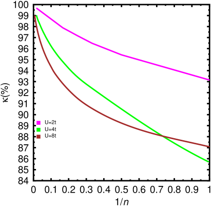
Figure 1: (Color online) The ratio of correlation energies $\kappa$ obtained with the FED approximation is plotted as a function of the inverse of the number of GHF transformations for a lattice with $N_{sites}$=30 sites and $N_{e}$=22 electrons. Results are shown for on-site repulsions of $U$=2$t$, 4$t$, and 8$t$. For details, see the main text.

However, being already more sophisticated than the SR framework, Carlos-Hubbard-1D ; PQT-reference-1 ; PQT-reference-2 ; PQT-reference-3 the extension Rayner-2D-Hubbard-PRB-2012 ; Carlos-Rayner-Gustavo-VAMPIR-molecules mentioned above still essentially describes a given ground and/or excited state in terms of a single symmetry-projected configuration. This certainly limits the amount of correlations that can be accessed for those states. A more correlated description is encoded in a MR scheme. Tomita-1 ; Tomita-2 ; Tomita-2011PRB ; rayner-Hubbard-1D-FED2013 Here, one resorts to a set of symmetry-broken HF states $|{\cal{D}}^{i}\rangle$ and superposes their Goldstone manifolds $\hat{R}|{\cal{D}}^{i}\rangle$. In this way, a given state with a well defined set of quantum numbers is expanded in terms of $n$ nonorthogonal symmetry-projected configurations Tomita-1 ; rayner-Hubbard-1D-FED2013 that are optimized with the help of the Ritz variational principle Blaizot-Ripka applied to the projected energy.

There are several ways to perform the self-consistent optimization of the intrinsic HF states $|{\cal{D}}^{i}\rangle$ within a MR approach. One possible VAP strategy is represented by the Resonating HF Tomita-1 ; Tomita-2 ; Tomita-2011PRB ; Fukutome-original-RSHF ; Yamamoto-1 ; Yamamoto-2 ; Ikawa-1993 (ResHF) scheme within which all the determinants $|{\cal{D}}^{i}\rangle$ are optimized at the same time. Another VAP strategy is represented by the Few Determinant rayner-Hubbard-1D-FED2013 ; Carlo-review (FED) approach where, the HF transformations ${\cal{D}}^{i}$ are optimized one-at-a-time. In both the ResHF and FED schemes, the corresponding configuration mixing coefficients are determined through resonon-like equations. Gutzwiller_method We note that there is no need for the FED expansion to be short, as its name would imply, although this is a desirable feature. In the present study, we keep the acronym to remain consistent with the literature. Carlo-review Hybrid MR approximations are also possible. For example, one could optimize $n-k$ states using the ResHF scheme and $k$ states using the FED one.

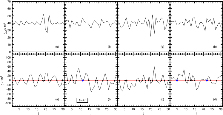
Figure 2: (Color online) The quantities ${\xi}^{i}(j)$ [panels (a) to (d)] and ${\xi}_{cd}^{i}(j)$ [(e) to (h)] are plotted for a 1D lattice with $N_{sites}$=30 sites and $N_{e}$=18 electrons at $U$=2$t$, as a function of lattice site $j$ for some typical symmetry-broken GHF determinants resulting from the FED VAP optimization. Results corresponding to the standard RHF approximation, are plotted in red for comparison. For more details, see the main text.

The FED methodology has already been used rayner-Hubbard-1D-FED2013 to compute ground state energies, spin-spin correlation functions (SSCFs) in real space, magnetic structure factors (MSFs) as well as spin-charge separation tendencies in the SFs of half-filled 1D Hubbard lattices of different sizes in the weak, intermediate-to-strong, and strong interaction regimes. We have shown Carlos-Rayner-Gustavo-FED-molecules that short ResHF and FED expansions can provide an accurate description of chemical systems such as the nitrogen and water molecules along the entire dissociation profile, as well as an accurate interconversion profile among the peroxo and bis($\mu$-oxo) forms of [Cu₂O₂]²⁺ comparable to other state-of-the-art quantum chemical methods. Recent calculations, Laimis-paper have also considered the complex binding pattern in the Mo₂ molecule.

In addition to ground state properties, the Excited Few Determinant Carlo-review (EXCITED FED) scheme has also been used rayner-Hubbard-1D-FED2013 to treat excited states, with well defined quantum numbers, as expansions in terms of nonorthogonal symmetry-projected configurations. As a byproduct of VAP calculations, the EXCITED FED provides a (truncated) basis consisting of a few Gram-Schmidt orthonormalized states, each of them expanded in a given number of nonorthogonal symmetry-projected configurations, which may be used to perform a final diagonalization of the Hamiltonian to account for a more correlated description of both ground and excited states.

Let us stress, that each of the MR approaches already mentioned has its own advantages and drawbacks. A ResHF wave function is stationary with respect to arbitrary changes in the HF transformations rs ${\cal{D}}^{i}$ (i=1, $\dots$, $n$) while a FED one displays stationarity only with respect to the last added transformation. Therefore, the ResHF wave functions become easier to work with in the evaluation of those properties depending on derivatives of the wave function. However, in a ResHF optimization, ${\cal{O}}(n^{2})$ Hamiltonian and norm kernels have to be recomputed at every iteration while only ${\cal{O}}(n)$ kernels are required in an efficient implementation of the FED method. rayner-Hubbard-1D-FED2013 ; Carlos-Rayner-Gustavo-FED-molecules

Regardless of the FED and/or ResHF VAP strategy adopted, the MR approximations are not restricted by the dimensionality (i.e., they can be equally well applied to 1D and 2D systems) and/or the topology of the considered lattices. On the other hand, one of the most attractive features of the MR approximations is that they offer compact wave functions, with well defined quantum numbers, whose quality can be systematically improved by increasing the number of symmetry-projected configurations included in the corresponding ansatz. Tomita-1 ; Tomita-2 ; Tomita-2011PRB ; rayner-Hubbard-1D-FED2013 ; Carlos-Rayner-Gustavo-FED-molecules Obviously, one is always limited in practical applications to a finite number $n$ of symmetry-projected terms in the FED and/or ResHF expansions. However, it should also be kept in mind that both the ResHF and FED wave functions are nothing else than a discretized form of the exact coherent state representation of a fermion state Perlemov and, therefore, become exact in the limit $n\rightarrow\infty$. All in all, we believe that symmetry-projected approximations, already quite successful in nuclear physics, rs ; Carlo-review ; rayner-GCM-paper ; rayner-GCM-parity lead to a rich conceptual landscape and deserve further attention in quantum chemistry PQT-reference-1 ; PQT-reference-2 ; PQT-reference-3 ; Carlos-Rayner-Gustavo-VAMPIR-molecules ; Carlos-Rayner-Gustavo-FED-molecules and condensed matter physics. Carlos-Hubbard-1D ; Rayner-2D-Hubbard-PRB-2012 ; non-unitary-paper-Carlos ; rayner-Hubbard-1D-FED2013 They also provide PaperwithShiwei high quality trial states that can be used within the constrained-path Monte Carlo CPMC-ref scheme, increasing the energy accuracy and decreasing the statistical variance as more symmetries are broken and restored.

In this paper we apply, for the first time, the FED approach to doped systems. Therefore, our main goal is to test its performance using benchmark calculations. To this end, we have selected the 1D Hubbard model for which both exact and highly accurate density matrix renormalization group (DMRG) results can be obtained. For the sake of completeness and comparison we will also discuss half-filling results. In Sec. II, we briefly describe the key ingredients of our MR approach. For a more detailed account, the reader is referred to our previous works. rayner-Hubbard-1D-FED2013 ; Carlos-Rayner-Gustavo-FED-molecules In Sec. III, we discuss the results of our calculations. We have first paid attention to lattices with $N_{sites}$=30 sites and $N_{e}$=14, 18, 22, 26, 30 electrons as illustrative examples. Calculations have been performed for the on-site repulsions $U$=2$t$, 4$t$, and 8$t$ representing the weak, intermediate-to-strong (i.e., noninteracting band width), and strong interaction regimes, respectively. In Sec. III.1, we compare our ground state and correlation energies with the exact ones as well as with those obtained using other theoretical methods. The dependence of the correlation energies predicted for doped lattices with the number of transformations included in our MR ansatz is also discussed in the same section. The basic units of quantum fluctuations in the case of doped lattices are discussed in Sec. III.2, where we consider the structure of the symmetry-broken determinants resulting from the FED VAP procedure. Next, in Secs. III.3 and III.4, we benchmark our results for momentum distributions, SSCFs, and density-density (DDCFs) correlation functions with DMRG ones obtained with the open-source ALPS software. ALPS A typical outcome of our calculations for SFs and DOS ${\cal{N}}(\omega)$ is presented in Sec. III.5, where we consider a lattice with $N_{sites}$=30 sites and $N_{e}$=26 electrons at $U$=4$t$. Next, in Sec. III.6, we illustrate the performance of the FED method in the case of larger lattice sizes. Finally, Sec. IV is devoted to the concluding remarks and work perspectives.

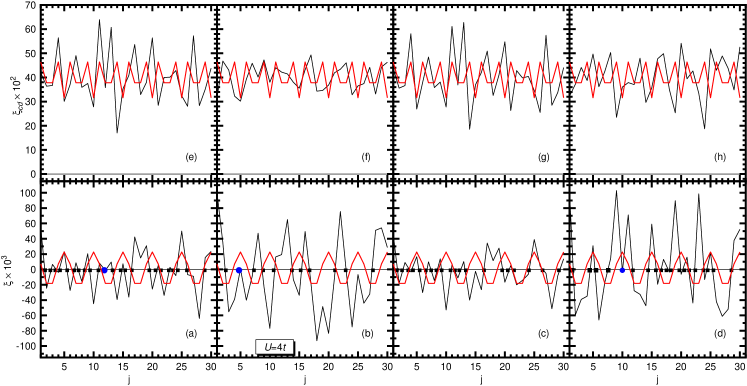
Figure 3: (Color online) Same as Fig. 2 but for $U$=4$t$. Results corresponding to the standard UHF approximation, are plotted in red for comparison.

II Theoretical Framework

We consider the 1D Hubbard Hamiltonian Hubbard-model_def1

$$\hat{H}=-t\sum_{j,\sigma=\uparrow,\downarrow}\Big{\{}\hat{c}_{j+1\sigma}^{\dagger}\hat{c}_{j\sigma}+\hat{c}_{j\sigma}^{\dagger}\hat{c}_{j+1\sigma}\Big{\}}+U\sum_{j}\hat{n}_{j\uparrow}\hat{n}_{j\downarrow}$$ (1)

where the first term represents the nearest-neighbor hopping (t $>$ 0) and the second is the repulsive on-site interaction (U $>$ 0). The fermionic Blaizot-Ripka spin-1/2 operators $\hat{c}_{j\sigma}^{\dagger}$ and $\hat{c}_{j\sigma}$ create and destroy an electron with spin-projection $\sigma=\uparrow,\downarrow$ on a lattice site j=1, $\dots$, $N_{sites}$. The operators $\hat{n}_{j\sigma}$ = $\hat{c}_{j\sigma}^{\dagger}\hat{c}_{j\sigma}$ are the local number operators. We assume periodic boundary conditions and a lattice spacing $\Delta$=1.

The starting point rayner-Hubbard-1D-FED2013 of our FED approach is a set of GHF determinantsStuberPaldus ; HFclassification $|{\cal{D}}^{i}\rangle$ ($i=1,\dots$, n), which deliberately break several symmetries of the Hamiltonian like rotational (in spin space) and spatial ones. To restore these broken symmetries, we explicitly use the spin

$$\hat{P}_{\Sigma{\Sigma}^{{}^{\prime}}}^{S}=\frac{2S+1}{8{\pi}^{2}}\int d\Omega{\cal{D}}_{\Sigma{\Sigma}^{{}^{\prime}}}^{S*}(\Omega)R(\Omega)$$ (2)

and space group

$$\hat{P}_{mm^{{}^{\prime}}}^{k}=\frac{h}{L}\sum_{g=1}^{L}{\Gamma}_{mm^{{}^{\prime}}}^{k*}(g)\hat{R}(g)$$ (3)

projection operators. rayner-Hubbard-1D-FED2013 In Eq.(2), $R(\Omega)$ is the rotation operator in spin space, the label $\Omega$ stands for the set of Euler angles, and ${\cal{D}}_{\Sigma{\Sigma}^{{}^{\prime}}}^{S}(\Omega)$ are Wigner matrices. Edmonds In Eq.(3), $h$ and $L$ represent the dimension of the irreducible representation and the number of space group operations for a given lattice. On the other hand, ${\Gamma}_{mm^{{}^{\prime}}}^{k}(g)$ is an irreducible representation Tomita-1 ; Lanczos-Fano while $\hat{R}(g)$ represents the corresponding point group symmetry operations parametrized in terms of the label g. The linear momentum ${k}=\frac{2\pi}{N_{sites}}{\xi}$ is given in terms of the quantum number $\xi$ which takes the values allowed inside the Brillouin zone (BZ). Ashcroft-Mermin-book The high symmetry momenta $k$=0,$\pi$ are also labelled by the parity of the corresponding irreducible representation. Tomita-1 ; Lanczos-Fano In what follows we will not explictly write this label. The total projection operator can then be written in the following shorthand form

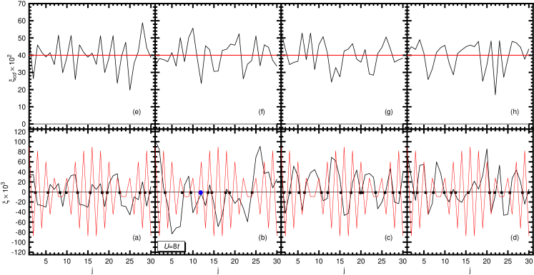
Figure 4: (Color online) Same as Fig. 2 but for $U$=8$t$. Results corresponding to the standard GHF approximation, are plotted in red for comparison.

$$\hat{P}_{\Sigma{\Sigma}^{{}^{\prime}}}^{S}\hat{P}_{mm^{{}^{\prime}}}^{k}=\hat{P}_{KK^{{}^{\prime}}}^{\Theta}$$ (4)

where $\Theta=(S,k)$ represents the set of (spin and linear momentum) symmetry quantum numbers and $K=(\Sigma,m)$. The key idea of the FED approach is to superpose the set of degenerate Goldstone states rayner-Hubbard-1D-FED2013 $|{\cal{D}}^{i}(\Omega,g)\rangle=\hat{R}(\Omega)\hat{R}(g)|{\cal{D}}^{i}\rangle$ through the following ansatz

$$|\phi_{K}^{n\Theta}\rangle=\sum_{K^{{}^{\prime}}}\sum_{i=1}^{n}f_{K^{{}^{\prime}}}^{i\Theta}\hat{P}_{KK^{{}^{\prime}}}^{\Theta}|{\cal{D}}^{i}\rangle$$ (5)

which expands a given ground state $|\phi_{K}^{n\Theta}\rangle$, with well defined symmetry quantum numbers $\Theta$, in terms of $n$ nonorthogonal symmetry-projected configurations $\hat{P}_{KK^{{}^{\prime}}}^{\Theta}|{\cal{D}}^{i}\rangle$. The sum over $K^{{}^{\prime}}$ in Eq.(5) is necessary in order to remove an unphysical dependence of $|\phi_{K}^{n\Theta}\rangle$ on the orientation of the GHF states $|{\cal{D}}^{i}\rangle$. Schmid-Gruemmer-1984

The FED wave function is formally similar to the one adopted within the ResHF method. Tomita-1 ; Tomita-2 ; Tomita-2011PRB ; Fukutome-original-RSHF ; Yamamoto-1 ; Yamamoto-2 ; Ikawa-1993 It is determined by applying the Ritz variational principle Blaizot-Ripka to the energy (independent of K)

$$E^{n\Theta}=\frac{f^{n\Theta\dagger}{\cal{H}}^{n\Theta}f^{n\Theta}}{f^{n\Theta\dagger}{\cal{N}}^{n\Theta}f^{n\Theta}}$$ (6)

written in terms of Hamiltonian and norm kernels

$${\cal{H}}_{iK,jK^{{}^{\prime}}}^{n\Theta} = \langle{\cal{D}}^{i}|\hat{H}\hat{P}_{KK^{{}^{\prime}}}^{\Theta}|{\cal{D}}^{j}\rangle$$

$${\cal{N}}_{iK,jK^{{}^{\prime}}}^{n\Theta} = \langle{\cal{D}}^{i}|\hat{P}_{KK^{{}^{\prime}}}^{\Theta}|{\cal{D}}^{j}\rangle$$ (7)

which require the knowledge of the symmetry-projected matrix elements between all the GHF determinants used in the expansion Eq.(5). In the case of the mixing coefficients, we obtain a resonon-like Gutzwiller_method eigenvalue equation

$$\left({\cal{H}}^{n\Theta}-E^{n\Theta}{\cal{N}}^{n\Theta}\right)f^{\Theta}=0$$ (8)

with the constraint $f^{n\Theta\dagger}{\cal{N}}^{n\Theta}f^{n\Theta}=1$ ensuring the normalization of the solution. Within the FED approach the energy Eq.(6) is varied only with respect to the last added GHF determinant $|{\cal{D}}^{n}\rangle$ keeping all the other transformations ${\cal{D}}^{i}$ (i=1, $\dots$, $n-1$), obtained in previous chains of VAP calculations, fixed. rayner-Hubbard-1D-FED2013 Note that at variance with the ResHF approximation, Tomita-1 ; Tomita-2 ; Tomita-2011PRB ; Fukutome-original-RSHF ; Yamamoto-1 ; Yamamoto-2 ; Ikawa-1993 where all the transformations ${\cal{D}}^{i}$ are optimized at the same time, the FED VAP strategy optimizes them one-at-a-time. This is particularly relevant for alleviating our numerical effort if one keeps in mind that we use the most general symmetry-broken GHF states and therefore a full 3D spin projection Eq.(2) is required. Regardless of the adopted FED and/or ResHF strategy, the variation with respect to the transformations ${\cal{D}}^{i}$ can be efficiently parametrized with the help of the Thouless theorem. Rayner-2D-Hubbard-PRB-2012 ; Carlos-Hubbard-1D ; non-unitary-paper-Carlos ; rayner-Hubbard-1D-FED2013 ; Carlos-Rayner-Gustavo-VAMPIR-molecules ; Carlos-Rayner-Gustavo-FED-molecules

All the FED calculations discussed in this paper have been carried out with an in-house parallel implementation rayner-Hubbard-1D-FED2013 of our VAP procedure. We have used a limited-memory quasi-Newton method quasi-Newton to handle the optimization. Note that the FED expansion of a given ground state $|\phi_{K}^{n\Theta}\rangle$ by $n$ nonorthogonal symmetry-projected GHF configurations enlarges the flexibility in our wave functions, with respect to a SR description, to a total number $n_{var}=2n(2N_{sites}-N_{e})\times N_{e}+4nS+2(n-1)$ of variational parameters.

In Sec. III.5, we will also discuss both the SFs and DOS ${\cal{N}}(\omega)$. The key point, is to superpose the Goldstone hole $|{\cal{D}}_{h}^{i}\left(\Omega,g\right)\rangle=\hat{R}(\Omega)\hat{R}(g){\hat{b}}_{h}\left({\cal{D}}^{i}\right)|{\cal{D}}^{i}\rangle$ and particle $|{\cal{D}}_{p}^{i}\left(\Omega,g\right)\rangle=\hat{R}(\Omega)\hat{R}(g){\hat{b}}_{p}^{\dagger}\left({\cal{D}}^{i}\right)|{\cal{D}}^{i}\rangle$ (i= 1, $\dots$, $n_{T}$) manifolds in the wave functions of the $N_{e}-1$ and $N_{e}+1$ electron systems, respectively. The amplitudes of these superpositions are then determined through the corresponding generalized eigenvalue equations similar to Eq.(8). With these ingredients at hand, as well as the FED solution $|\phi_{K}^{n\Theta}\rangle$, the SFs and DOS can be computed according to Eqs.(25) and (26) in our previous work.rayner-Hubbard-1D-FED2013

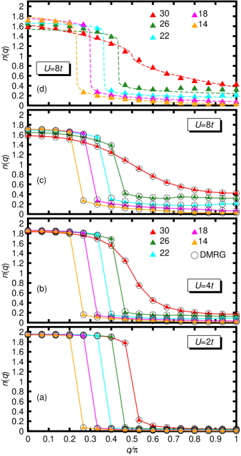
Figure 5: (Color online) The ground state momentum distributions Eq.(12) for $N_{sites}$=30 lattices with 14 (orange triangles), 18 (magenta triangles), 22 (cyan triangles), 26 (green triangles), and 30 (red triangles) electrons are shown for $U$=2$t$ (a), 4$t$ (b), and 8$t$ (c). DMRG results (open black circles) are also included in panels (a) to (c) for comparison. The FED values (filled triangles) are compared in panel (d) with a power-law [Eq.(13)] fitting (dashed lines) of the momentum distributions.

Finally, for the convenience of the reader we summarize the acronyms used in the present study for different types of Slater determinants:

• RHF is used for those symmetry-adapted states preserving all the symmetries of the Hamiltonian Eq.(1).

• UHF is used for those states preserving the $\hat{S}_{z}$-symmetry while possibly breaking all others.

• GHF states are those that break all the symmetries of the considered Hamiltonian.

III Discussion of results

In this section, we discuss the results of our FED calculations. First, we pay attention to lattices with $N_{sites}$=30 sites and $N_{e}$=14, 18, 22, 26, 30 electrons. Results are presented for on-site repulsions $U$=2$t$, 4$t$, and 8$t$, respectively. In Sec. III.1, we compare the ground state and correlation energies with the exact ones, as well as with results obtained using other theoretical approaches. We also discuss, for the case of doped lattices, the dependence of the correlation energies on the number $n$ of nonorthogonal symmetry-projected GHF configurations. Next, in Sec. III.2, we consider the structure of the intrinsic GHF determinants resulting from our VAP procedure in the case of doped lattices. The momentum distributions are presented in Sec. III.3 while the Fourier transforms of the SSCFs and DDCFs in real space are shown in Sec. III.4. They are compared with those obtained within the DMRG framework retaining 1024 states in the renormalization procedure. On the other hand, in Sec. III.5, we discuss spin-charge separation tendencies in the SFs and DOS ${\cal{N}}(\omega)$ of a lattice with $N_{sites}$=30 sites and $N_{e}$=26 electrons. Finally, in Sec. III.6, we illustrate the performance of the FED method in the case of larger lattices.

III.1 Ground state and correlation energies

In Table 1, we compare the exact LIEB ; BETHE and the predicted FED ground state energies for half-filled and doped lattices with $N_{sites}$=30 sites and $N_{e}$=14, 18, 22, 26, 30 electrons. The corresponding $\Theta$ = (0,0) ground states have A₁ symmetry, i.e., they are symmetric under the reflection $x\rightarrow-x$. For $U$=2$t$ and 4$t$, the FED energies shown in the table have been obtained by including $n$=60 nonorthogonal symmetry-projected GHF configurations in the ansatz Eq.(5). On the other hand, $n$=150 GHF transformations have been used for $U$=8$t$. Besides the RHF energies, we have included in Table 1 the lowest possible HF solution for completeness. At $U$=2$t$, the lowest-energy HF solution coincides with the RHF one in the case of doped systems while an UHF solution is obtained at half-filling. At $U$=4$t$ the HF state corresponds to an UHF wave function while for $U$=8$t$ we have found a GHF solution with predominant ferromagnetic character. In the same table, we also show our previous results rayner-Hubbard-1D-FED2013 (FED^∗), based on $n$=25 GHF transformations, and the ResHF ones Tomita-1 obtained with $n$=30 UHF transformations. We have computed the ratio

$$\kappa_{FED}=\frac{E_{RHF}-E_{GHF-FED}}{E_{RHF}-E_{Exact}}\times 100$$ (9)

in order to check how well the FED correlation energies reproduce the exact ones. For the other approximations, such a ratio is obtained from a similar expression.

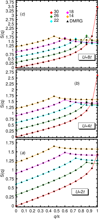
Figure 6: (Color online) Fourier transforms of the ground state spin-spin correlation functions in real space for $N_{sites}$=30 lattices with 14 (orange diamonds), 18 (magenta diamonds), 22 (cyan diamonds), 26 (green diamonds), and 30 (red triangles) electrons are shown for $U$=2$t$ (a), 4$t$ (b), and 8$t$ (c). DMRG results (black triangles) are also included for comparison. Starting with 26 electrons, all the curves have been successively shifted by 0.3 to accomodate them in a single plot.

The first noticeable feature from Table 1 is that, at most, the standard HF solutions account for 93.65 $\%$ of the exact correlation energy. Regardless of the filling and/or the interaction strength, the MR FED expansion clearly recovers a very large portion of correlation energy (i.e., $\kappa_{FED}$ $\geq$ 99 $\%$) in all cases studied. For the half-filled case as well as for the lattices with 26 and 22 electrons, the ground state and correlation energies improve the ResHF and FED^∗ ones obtained in previous studies. Tomita-1 ; rayner-Hubbard-1D-FED2013 On the other hand, the DMRG energies (not shown in the table) are exact to all the quoted figures. We have further used the DMRG results in Secs. III.3 and III.4 to benchmark our calculations for momentum distributions and correlation functions.

From these results and the ones obtained in our previous work, rayner-Hubbard-1D-FED2013 we conclude that the FED scheme provides a reasonable starting point to obtain correlated ground state wave functions, with well defined symmetry quantum numbers, in both half-filled and doped 1D Hubbard lattices. In addition, the method offers a systematic way to improve, through chains of VAP calculations, the quality of such wave functions by increasing the number $n$ of nonorthogonal symmetry-projected GHF configurations included in the FED ansatz. This is illustrated in Fig. 1 where we have plotted, as a function of the inverse $1/n$ of the number of transformations, the ratio $\kappa_{FED}$ for a doped lattice with $N_{sites}$=30 sites and $N_{e}$=22 electrons. One sees that $\kappa_{FED}$ increases smoothly and approaches the exact result as the number of symmetry-projected configurations is increased. For example, a single symmetry-projected configuration provides $\kappa_{FED}$=93.14 $\%$, 85.67 $\%$, 87.08 $\%$ while increasing the number of GHF transformations up to $n$=10 we obtain $\kappa_{FED}$=98.37 $\%$, 96.23 $\%$ and 94.35 $\%$ for $U$=2$t$, 4$t$ and 8$t$, respectively.

Some comments are in order here. First, since the nature of the quantum correlations varies for different doping fractions $x=N_{e}/N_{sites}$ and on-site repulsions, one can expect that the number of GHF transformations required to obtain a given $\kappa_{FED}$ ratio depends on both of them. As already mentioned the FED wave functions become exact in the limit $n\rightarrow\infty$. In practice we are always limited to a finite number of nonorthogonal symmetry-projected configurations in the FED expansion and it is difficult to assert beforehand how many of them are required. Therefore, their number $n$ should be tailored, through chains of VAP calculations, so as to reach a reasonable accuracy not only in the ground state energy but also in other physical quantities like, for example, the spin-spin correlators. In the present study we have used a fixed number $n$=60 for both the weak and intermediate-to-strong interaction regimes while a larger number $n$=150 is required to obtain the energies reported in Table 1 at $U$=8$t$. As we will see later on in Sec. III.4, a larger number of transformations is also required, especially close to half-filling, to improve the quality of the predicted correlation functions. This can be qualitatively understood from the crossover in the SSCFs CrossOverSS that explains how the antiferromagnetic spin correlation at half-filling grows near half-filling. One may then expect strong quantum fluctuations near half-filling, whose basic units (see, Sec. III.2) can only be captured with larger FED expansions. The performance of the FED method for larger lattices will be discussed in Sec. III.6.

III.2 Structure of the intrinsic determinants and basic units of quantum fluctuations in doped lattices

In our previous study rayner-Hubbard-1D-FED2013 of the half-filled 1D Hubbard model we have considered two orders parameters, i.e., the spin density (SD)

$$\xi(j)=(-)^{j-1}\langle{\cal{D}}|\hat{\bf{S}}(j)|{\cal{D}}\rangle\cdot\langle{\cal{D}}|\hat{\bf{S}}(1)|{\cal{D}}\rangle$$ (10)

and the charge density (CD)

$${\xi}_{cd}(j)=1-\sum_{\sigma}\langle{\cal{D}}|\hat{n}_{j\sigma}|{\cal{D}}\rangle$$ (11)

associated with an arbitrary symmetry-broken determinant $|{\cal{D}}\rangle$, with j=1, $\dots$, $N_{sites}$ being the lattice index. The comparison of the SD and CD computed with the standard UHF solution and the ones obtained using the GHF determinants $|{\cal{D}}^{i}\rangle$ resulting from the FED VAP procedure, reveals that ${\xi}^{i}(j)$ displays neutral [i.e., ${\xi}_{cd}^{i}(j)$=0] solitons Horovitz whose translational and breathing motions can be regarded Tomita-1 ; rayner-Hubbard-1D-FED2013 ; Yamamoto-1 ; Ikawa-1993 as the basic units of quantum fluctuations in the FED wave functions Eq.(5).

The question naturally arises, as to what are the basic units of the quantum fluctuations captured within the FED VAP optimization in the case of doped 1D lattices. Among all the GHF transformations ${\cal{D}}^{i}$ used to describe the lattice with $N_{sites}$=30 sites and $N_{e}$=18 electrons (see, Sec. III.1), we have selected some typical examples to plot in Figs. 2, 3 and 4 the corresponding SD ${\xi}^{i}(j)$ [panels (a) to (d)] and CD ${\xi}_{cd}^{i}(j)$ [panels (e) to (h)] as functions of lattice site. Results obtained with the lowest-energy standard HF solutions are also included in the plots (red) for comparison.

In the case of the RHF solution (Fig.2) at $U$=2$t$, the corresponding SD vanishes while the CD takes the constant value 0.4. Due to the symmetry-broken nature of the UHF solution (Fig.3), the corresponding SD and CD exhibit oscillating patterns around the expected values (i.e., 0 and 0.4, respectively) at $U$=4$t$. In the case of the intrinsic GHF solution (Fig.4) at $U$=8$t$ the SD displays a very fast oscillating pattern, which is a direct consequence of its predominant ferromagnetic character [note the presence of the factor $(-)^{j-1}$ in the definition Eq.(10)]. In fact, the energy of this intrinsic GHF solution (i.e, -18.1922 t) is only slightly lower than the one (i.e., -18.0974 t) corresponding to a fully ferromagnetic UHF solution with all the spins aligned along the z-direction. On the other hand, the CD takes the constant value 0.4.

Regardless of the considered interaction regime, the GHF determinants $|{\cal{D}}^{i}\rangle$ associated with the FED solution Eq.(5) exhibit pairs of solitons (black squares) where the SD ${\xi}^{i}(j)$ changes its sign. The space group projection operator provides a translational motion for such soliton pairs. When different determinants show soliton pairs with different widths, this can be interpreted as a breathing mechanism. Isolated points (blue circles) where ${\xi}^{i}(j)$ becomes zero are also apparent from Figs. 2, 3 and 4. In the case of doped lattices these new defects represent polarons. Tomita-1 In addition, the CD ${\xi}_{cd}^{i}(j)$ displays local variations around the constant value 0.4 for all the considered on-site repulsions. Other GHF determinants $|{\cal{D}}^{i}\rangle$ (not shown in the figures) display the same qualitative features. Similar results also hold for other U values and lattices.

Therefore, in the case of doped 1D lattices, the ansatz Eq.(5) superposes manifolds $|{\cal{D}}^{i}\left(\Omega,g\right)\rangle=\hat{R}(\Omega)\hat{R}(g)|{\cal{D}}^{i}\rangle$ containing both solitons and polarons. One is then left with an intuitive physical picture Tomita-1 ; rayner-Hubbard-1D-FED2013 in which the basic units of quantum fluctuations in 1D lattices can be mainly associated with the translational and breathing motions of neutral and charged solitons. However, in the case of doped 1D systems, a part of such fluctuations can also be described by polarons. Within both the FED rayner-Hubbard-1D-FED2013 and the ResHF Tomita-1 ; Yamamoto-1 ; Ikawa-1993 schemes, the interference between the defects belonging to different symmetry-broken determinants $|{\cal{D}}^{i}\rangle$ is accounted for through Eq.(8).

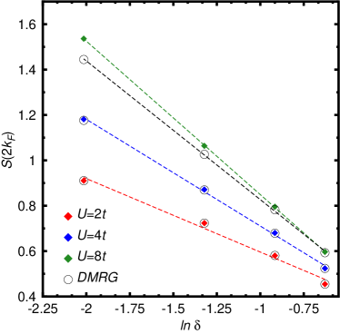
Figure 7: (Color online) Maxima of Fourier transforms of the FED ground state spin-spin correlation functions in real space [Eq.(14)] plotted as functions of ln $\delta$, with $\delta$ being the corresponding doping parameter. Results are shown for on-site repulsions $U$=2$t$ (red diamonds), 4$t$ (blue diamonds), and 8$t$ (green diamonds). DMRG values are plotted with open circles. A straight line has been fitted to guide the eye. For more details, see the main text.

III.3 Momentum distribution

For a given set of quantum numbers $\Theta$, the momentum distribution $n^{n\Theta}(q)$ can be computed as

$$n^{n\Theta}(q)=\sum_{\sigma}\frac{\langle\phi_{K}^{n\Theta}|{\hat{n}}_{q\sigma}|\phi_{K}^{n\Theta}\rangle}{\langle\phi_{K}^{n\Theta}|\phi_{K}^{n\Theta}\rangle}$$ (12)

where $\hat{n}_{q\sigma}$ is the $\sigma$-occupation operator at wave vector q. Note that, due to the particular form of the operator $\hat{n}_{q\sigma}$, the momentum distribution Eq.(12) does not depend explicitly on $K$.

The ground state momentum distributions for $N_{sites}$=30 lattices with 14 (orange triangles), 18 (magenta triangles), 22 (cyan triangles), 26 (green triangles), and 30 (red triangles) electrons are plotted in panels (a), (b) and (c) of Fig. 5 for on-site repulsions $U$=2$t$, 4$t$, and 8$t$, respectively. Regardless of the interaction strength, the FED and DMRG (open black circles) momentum distributions agree well. In all cases, we have obtained a jump at $q=k_{F}$, with $k_{F}$ being the Fermi momentum, that becomes less pronounced, especially at half-filling, for larger U values. Such a jump is also found in calculations based on the exact solution at $U$=$\infty$ Ogata-Shiba as well as in previous studies. Sorella-1990 ; Qin-S2kf As can seen from panel (c), the momentum distribution presents a slight nonmonotonic behavior close to half-filling (i.e., $N_{e}$=26) due to a small feature near $q=2k_{F}$.

Previous works Ogata-Shiba ; Sorella-1990 ; Qin-S2kf ; Solyom ; SchulzPRL1990 have shown that, contrary to an ordinary Fermi liquid, the momentum distribution of the 1D Hubbard model exhibits a power-law behavior around $q=k_{F}$ given by

$$n(q)=n(k_{F})+C|q-k_{F}|^{\tau}\text{sgn}\left(q-k_{F}\right)$$ (13)

at half-filling or U $\to$ $\infty$. We have used the momentum distributions obtained with the FED approach to fit the functional dependence Eq.(13). The results are shown in panel (d) of Fig. 5 for $U$=8$t$. Despite the fact that the functional form Eq.(13) has been obtained using the exact $U$=$\infty$ solution, we observe that it nicely reproduces the trends in the FED (and also DMRG) results.

III.4 Correlation functions

Let us now turn our attention to the predicted FED SSCFs and DDCFs. We compare them with the corresponding DMRG values in the case of $N_{sites}$=30 lattices with 14 (orange triangles), 18 (magenta triangles), 22 (cyan triangles), 26 (green triangles), and 30 (red triangles) electrons. This comparison will allow us to reveal to which extent the FED scheme can capture the main short, medium and long range features in these correlators, especially in the case of doped lattices. We have resorted to the momentum space representation (i.e., the Fourier transforms) of the SSCFs and DDCFs in real space. For a discussion of the predicted FED SSCFs in the case of half-filled lattices, the reader is also referred to our previous work. rayner-Hubbard-1D-FED2013

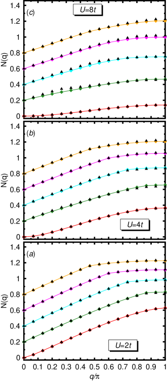
Figure 8: (Color online) Same as Fig. 6 but for the Fourier transforms of the ground state density-density correlation functions in real space. Starting with 26 electrons, all the curves have been successively shifted by 0.2 to accomodate them in a single plot.

The SSCFs in real space are given by

$$S_{m}^{n\Theta}(j)=\frac{\langle\phi_{K}^{n\Theta}|\hat{\bf{S}}(j)\cdot\hat{\bf{S}}(1)|\phi_{K}^{n\Theta}\rangle}{\langle\phi_{K}^{n\Theta}|\phi_{K}^{n\Theta}\rangle}$$ (14)

where the subindex $m$ accounts for the dependence with respect to the particular row of the space group irreducible representation used in the projection. Let us stress that the wave functions $|\phi_{K}^{n\Theta}\rangle$ Eq.(5) are pure spin states where orbital relaxation is allowed. Both conditions have already been shown to be important ingredients to improve the description of the long-range behavior of the SSCFs. Tomita-1 ; rayner-Hubbard-1D-FED2013 ; Yamamoto-1 ; Ikawa-1993 The Fourier transforms (FT-SSCFs) $S_{m}^{n\Theta}(q)$ of the SSCFs Eq.(14) are depicted in panels (a), (b) and (c) of Fig. 6 for the ground states of the lattices considered in the present study at $U$=2$t$, 4$t$ and 8$t$, respectively.

The first feature apparent from Fig. 6, is the prominent antiferromagnetic peak at the wave vector q=$\pi$ in the case of the half-filled system. The peaks of the FT-SSCFs always occur at $q=2k_{F}$. Such peaks have also been found Ogata-Shiba with the exact $U$=$\infty$ solution of the 1D Hubbard model as well as in previous calculations. Hirsch-S2kf ; Qin-S2kf ; Imada-S2kf They are shifted towards smaller linear momenta as we move away from half-filling. In the same plot, we have also included the results of our DMRG calculations (black triangles) for comparison. It is satisfying to observe that the predicted FED values closely follow the trend obtained within the DMRG approach. The largest differences between the FED and DMRG FT-SSCFs arise in the values of the corresponding peaks near half-filling for large U. For the lattice with 26 electrons the FED peak, obtained with $n$=150 GHF transformations, at $U$=8$t$ overestimates the DMRG one by 5 $\%$. On the other hand, using a smaller number $n$=60 of transformations, we obtain a poorer (10 $\%$ overestimation) description of the SSCFs and FT-SSCFs in the strong interaction regime.

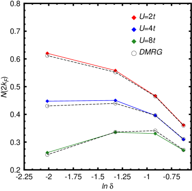
Figure 9: (Color online) Inflection points at wave vector $q=2k_{F}$ of the FED Fourier-transformed density-density correlation functions in real space [Eq.(15)] are plotted as functions of ln $\delta$ for $U$=2$t$ (red diamonds), 4$t$ (blue diamonds), and 8$t$ (green diamonds). DMRG values are plotted with open circles. For more details, see the main text.

A previous study CrossOverSS has shown the universal character of the crossover in the SSCFs as we approach half-filling. As a result of this crossover, the peaks observed in the FT-SSCFs at $q=2k_{F}$ display a linear logarithmic dependence with the doping parameter $\delta=1-x$. The results of our FED calculations are compared in Fig. 7 with the DMRG ones. For each U value, we have fitted a straight line to guide the eye. For $U$=2$t$ and 4$t$, the FED and DMRG values agree well (we have therefore included only the fitting of the former in the plot) and exhibit an almost linear behavior as a function of ln $\delta$. The same linear trend is observed at $U$=8$t$ though in this case the discrepancy between the FED and DMRG values, arising from a poorer description of the FT-SSCFs in the former (see, Fig. 6), is larger.

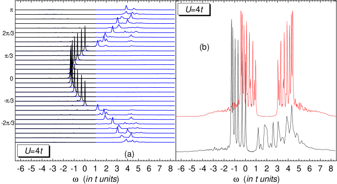
Figure 10: (Color online) The hole (black) and particle (blue) SFs for a lattice with $N_{sites}$=30 sites and $N_{e}$=26 electrons are plotted in panel (a) as functions of the excitation energy $\omega$ (in t units). The DOS (black) ${\cal{N}}(\omega)$ is compared in panel (b) with the one (red) corresponding to half-filling. The latter has been shifted (i.e., ${\cal{N}}(\omega)+40$) for the sake of clarity. Results are shown for the on-site repulsion $U$=4$t$. A Lorentzian folding of width $\Gamma$=0.05 t has been used. For more details, see the main text.

The DDCFs in real space can be computed as

$$N_{m}^{n\Theta}(j)=\frac{\langle\phi_{K}^{n\Theta}|\delta\hat{n}(j)\delta\hat{n}(1)|\phi_{K}^{n\Theta}\rangle}{\langle\phi_{K}^{n\Theta}|\phi_{K}^{n\Theta}\rangle}$$ (15)

where $\delta\hat{n}(j)=\hat{n}(j)-\langle\hat{n}(j)\rangle$ and $\hat{n}(j)=\sum_{\sigma}\hat{n}_{j\sigma}$. Their FT-DDCFs $N_{m}^{n\Theta}(q)$ are shown in panels (a), (b), and (c) of Fig. 8 for $U$=2$t$, 4$t$, and 8$t$, respectively. DMRG values (black triangles) are also plotted for comparison. Similar to the momentum distributions and FT-SSCFs already discussed above, the FED FT-DDCFs closely follow the trends observed in the DMRG ones, with the largest differences arising for $q\leq\pi/2$ in the case of the lattice with 26 electrons at $U$=8$t$. From panels (a), (b), and (c) of Fig. 8, we also observe the appearence of inflection points around $q=2k_{F}$ which become less pronounced as U increases. They are plotted in Fig. 9 as functions of ln $\delta$. We observe a shift down of the curves as U increases reflecting that the charge fluctuations decrease for larger U values. In addition, we note that the curves bend down more for larger on-site repulsions.

III.5 Spectral functions and density of states

A typical outcome of our calculations is shown in panel (a) of Fig. 10, where we have plotted the hole (black) and particle (blue) SFs, as functions of the excitation energy $\omega$, for a lattice with $N_{sites}$=30 sites and $N_{e}$=26 electrons at $U$=4$t$. Calculations have been performed along the lines described in our previous work. rayner-Hubbard-1D-FED2013 The FED ground state of the system with $N_{e}$=26 electrons has been approximated by $n$=60 GHF transformations while for the systems with $N_{e}\pm 1$ electrons we have superposed $n_{T}$=25 hole and particle manifolds (see, Sec. II). Smaller values $n_{T}$=5 and $n_{T}$=15 have also been investigated. However, increasing the number of hole and particle manifolds to $n_{T}$=25 leads to a shift of the main peaks and a redistribution of the strength of some of the peaks found for $n_{T}$=5 and $n_{T}$=15 as a result of the small number of configurations used in the calculations. In all cases, a Lorentzian folding of width $\Gamma$=0.05 t has been used.

We observe prominent hole peaks belonging to the spinon band. Such a band resembles the one found in the half-filled case rayner-Hubbard-1D-FED2013 though the spectral weight of some of the hole peaks found in the latter is redistributed to the particle sector due to the presence of doping. Another prominent feature of the SFs shown in panel (a) is the very extended distribution of the spectral weight for linear momenta $|k|>k_{F}$. The splitting of the strength in the corresponding particle SFs reveals that the present finite size results at the intermediate-to-strong interaction regime already display spin-charge separation tendencies beyond a simple quasiparticle distribution as well as shadow features. This agrees well with results obtained using other theoretical approximations. AraGo ; Senechal-scs ; PENcPRL1996

In panel (b) of Fig. 10 we have plotted the DOS ${\cal{N}}(\omega)$ corresponding to the lattice with $N_{sites}$=30 sites and $N_{e}$=26 electrons (black). For the sake of comparison, we have also included in the same panel the DOS in the half-filled case (red). The last one, has also been computed using $n$=60 and $n_{T}$=25. It exhibits the characteristic Hubbard gap moukouri2001 ; huscroft2001 ; aryanpour2003 ; AraGo and particle-hole symmetry. text-Hubbard-1D As can be seen from the figure, this particle-hole symmetry is lost in the doped case. As a result of states intruding the original gap, a smaller pseudogap is developed at $U$=4$t$. However, our calculations indicate that such a pseudogap progressively disappears for increasing doping fractions $x$. Similar results also hold for both $U$=2$t$ and $U$=8$t$ though the effect is less pronounced in the latter due to the larger value of the gap at half-filling.

Table 2: The ground state energies predicted within the FED scheme are compared with the exact ones. Results are presented for $N_{sites}$=34 lattices with $N_{e}$=14, 18, 22, 26, 30, 34 electrons as well as for the half-filled lattice with $N_{sites}$=50 sites. In each case, the number $n$ of transformations used in the FED ansatz [Eq.(5)] is indicated. The ratio of correlation energies $\kappa$, is computed according to Eq.(9)

$N_{sites}$		$N_{e}$		U		FED		$n$		Exact		$\kappa$ ($\%$)
34		14		4$t$		-23.0991		60		-23.1137		99.46
34		14		4$t$		-23.1048		100		-23.1137		99.67
34		18		4$t$		-26.4440		60		-26.4842		98.99
34		18		4$t$		-26.4587		100		-26.4842		99.35
34		22		4$t$		-27.8402		60		-27.9207		98.48
34		22		4$t$		-27.8673		100		-27.9207		98.99
34		26		4$t$		-27.1248		60		-27.2553		98.05
34		26		4$t$		-27.1634		100		-27.2553		98.63
34		30		4$t$		-24.2555		60		-24.3967		98.28
34		30		4$t$		-24.2966		100		-24.3967		98.78
34		34		4$t$		-19.4646		60		-19.5258		99.40
34		34		4$t$		-19.4876		100		-19.5258		99.62
34		34		8$t$		-11.0562		60		-11.1473		99.74
34		34		8$t$		-11.0883		100		-11.1473		99.83
50		50		2$t$		-42.1748		60		-42.2443		98.46
50		50		2$t$		-42.1957		100		-42.2443		98.62
50		50		4$t$		-28.1924		60		-28.6993		96.62
50		50		4$t$		-28.2999		100		-28.6993		97.33
50		50		8$t$		-15.7739		60		-16.3842		98.84
50		50		8$t$		-15.9770		100		-16.3842		99.22

III.6 Larger lattices

Now, we turn our attention to larger lattices. Let us stress that our aim in this section is not to be exhaustive but to illustrate the FED results in such lattices. To this end the predicted ground state energies are compared with the exact ones in Table II. Results are presented for $N_{sites}$=34 lattices with $N_{e}$=14, 18, 22, 26, 30, 34 electrons as well as for the half-filled lattice with $N_{sites}$=50 sites. For the considered on-site repulsions we have performed two different sets of FED calculations based on $n$=60 and $n$=100 GHF transformations. The ratio of correlation energies $\kappa$, has been computed according to Eq.(9).

As can be seen from the table, the FED approach, based on $n$=60 symmetry-projected configurations, already provides ${\kappa}_{FED}$ $>$ 98 $\%$. These values significantly improve the ones obtained with the standard HF approximation. For example, for the half-filled lattice with $N_{sites}$=50, the UHF approximation accounts for ${\kappa}_{UHF}$=12.02 $\%$, 65.02 $\%$, 92.26 $\%$ while ${\kappa}_{FED}$= 98.46 $\%$, 96.62 $\%$, 98.84 $\%$ at $U$=2$t$, 4$t$, and 8$t$, respectively. Note that, for the same on-site repulsions, the variational Monte Carlo method provides $\kappa$ values of around 87 $\%$, 92 $\%$, and 96 $\%$, respectively. Yokoyamma-Shiba For the same half-filled lattice, the ground state energies obtained with $n$=60 also improve the values reported in our previous work rayner-Hubbard-1D-FED2013 using a smaller number (i.e., $n$=25) of nonorthogonal symmetry-projected GHF configurations in the FED expansion Eq.(5) as well as the ones provided by the ResHF approximation Tomita-1 based on $n$=30 UHF transformations. Moreover, further increasing up to $n$=100 leads to ${\kappa}_{FED}$ $\geq$ 99.35 $\%$ in the case of lattices with $N_{sites}$=34 sites. In the case $N_{sites}=N_{e}$=50, we have obtained ${\kappa}_{FED}$= 98.62 $\%$, 97.33 $\%$, 99.22 $\%$ for $U$=2$t$, 4$t$, and 8$t$, respectively. The previous results show that the FED scheme also provides a resonable starting point to obtain correlated wave functions in lattices larger than the ones considered in Sec. III.1. In particular, one sees that for increasing lattice sizes the quality of the FED wave functions can also be systematically improved, for different doping fractions, by increasing the number of symmetry-projected configurations included in the MR ansatz Eq.(5). We are unable at the moment to anticipate the number of symmetry-projected configurations necessary to achieve a given quality in the FED wave functions for arbitrary lattice sizes and doping fractions. Nevertheless, we stress once more that the exact answer can always be approached in a systematic constructive way.

Finally, as a typical example of the results obtained for the lattices considered in this section, we have plotted in Fig. 11 the momentum distributions corresponding to $N_{sites}$=34 sites with 18 (magenta triangles), 26 (green triangles), and 34 (red triangles) electrons at $U$=4$t$. We have resorted to $n$=100 nonorthogonal symmetry-projected states in the calculations. As can be seen from the figure, the momentum distributions still display the main feature already discussed in Sec. III.3 for the case of half-filled and doped lattices with $N_{sites}$=30 sites, i.e., a jump at $q=k_{F}$ that becomes less pronounced at half-filling.

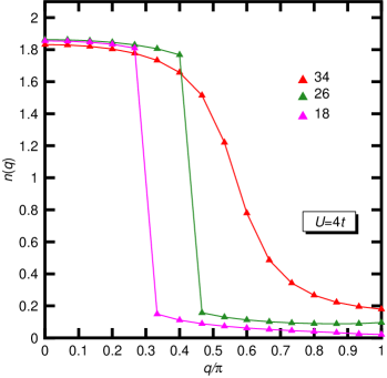
Figure 11: (Color online) The ground state momentum distributions Eq.(12) for $N_{sites}$=34 lattices with 18 (magenta triangles), 26 (green triangles), and 34 (red triangles) electrons are shown for $U$=4$t$.

IV conclusions

In the present study we have applied, for the first time, the FED approach to doped Hubbard systems. Our main goal has been to test its performance using benchmark calculations in 1D Hubbard lattices. Half-filled systems have also been discussed. We have compared the results of our calculations for ground state and correlation energies with those obtained using other theoretical approximations. From the results of our previous study rayner-Hubbard-1D-FED2013 and those obtained in the present work based on a larger number of nonorthogonal symmetry-projected GHF configurations in the MR expansion, we conclude that the FED scheme provides a reasonable starting point to obtain (compact) correlated wave functions in both half-filled and doped 1D Hubbard lattices. We have shown that the quality of such wave functions can be systematically improved, through chains of VAP calculations, in a constructive manner by increasing the number of transformations in the corresponding FED ansatz.

The analysis of the structure of the (intrinsic) symmetry-broken Slater determinants resulting from our VAP procedure reveals that they differ from that provided by the standard HF approximation. In particular, in the case of doped lattices they contain defects (i.e., solitons and polarons). The translational and breathing motions of such solitons can be regarded as the basic units of quantum fluctuations for the considered lattices. In addition, in the case of doped 1D systems, a part of the quantum fluctuations can also be described by polarons. On the other hand, though the FED results are not as accurate as the DMRG ones for the considered 1D lattices, our benchmark calculations for momentum distributions and correlations functions show that the former captures the main physics trends found in the latter.

We have also shown that the FED scheme can be used to access dynamical properties of doped 1D Hubbard lattices such as SFs and the DOS. To this end, in addition to the corresponding FED ground state based on $n$ GHF transformations, we have considered ansätze for the $N_{e}+1$ and $N_{e}-1$ electron systems that superpose $n_{T}$ particle and hole manifolds, respectively. For the case of a doped lattice with $N_{sites}$=30 sites and $N_{e}$=26 electrons our scheme provides hole and particle SFs that qualitatively agree with results obtained using other theoretical frameworks. They point point to a distribution of the spectral strength beyond the one expected for a simple quasiparticle distribution and display spin-charge separation tendencies in all the considered interaction regimes.

We believe that the finite size FED calculations already show that VAP MR expansions, based on nonorthogonal symmetry-projected Slater determinants, represent a useful theoretical tool to study low-dimensional correlated electronic systems with different doping contents that complement other existing approaches and could even be combined with them. Within this context, we have recently used PaperwithShiwei SR symmetry-projected wave functions as trial states within the constrained-path Monte Carlo framework. It has been shown that the use of such SR symmetry-projected states increases the energy accuracy while decreasing the statistical variance in calculations for large lattices. Given the fact that short FED-like expansions encode a more correlated description of the considered systems, they might be seen as plausible candidates for further improving the previous results.

The MR expansions used in the present study still offer a rich conceptual landscape for further development. In particular, small vibrations around symmetry-projected mean fields (i.e., symmetry-projected Tamm Dancoff and Random Phase approximations) can be consistently formulated. Scmid-RPA ; Nishiyama-RPA Such approximations can then be used to access a large number of excited states as required in studies of the optical conductivity in lattice models. optical-Dagotoo ; optical-Scalapino ; Jeckelmann Such calculations are in progress and will be reported elsewhere.

Let us stress that symmetry-projected approximations are not restricted by the dimensionality of the considered lattices. In this respect, our studies have paved the way for applying the MR methodology to the systematic description of both ground and excited states of 2D square, honeycomb, Kagome, and triangular lattices, as well as more involved multi-orbital Hubbard models relevant to iron-based superconductors. Dagotto-Rev-Mod-Physics-2013 In the realm of quantum chemistry, we plan to further enlarge our current developments Carlos-Rayner-Gustavo-VAMPIR-molecules ; Carlos-Rayner-Gustavo-FED-molecules for the molecular Hamiltonian.

- (1) E. Dagotto, Rev. Mod. Phys. 66, 763 (1994).
- (2) E. Dagotto, Rev. Mod. Phys. 85, 849 (2013).
- (3) J. G. Bednorz and K. A. Müller, Z. Phys. B 64, 189 (1986).
- (4) J. Hubbard, Proc. R. Soc. (London) A 276, 238 (1963).
- (5) D. Vollhardt, Rev. Mod. Phys. 56, 99 (1984).
- (6) P. W. Anderson, Science 235, 1196 (1987).
- (7) E. Dagotto, Science 309, 257 (2005).
- (8) Y. Kamihara, T. Watanabe, M. Hirano and H. Hosono, J. Am. Chem. Soc. 130, 3296 (2008).
- (9) G. R. Stewart, Rev. Mod. Phys. 83, 1539 (2011).
- (10) P. Dai, J. Hu and E. Dagotto, Nature 8, 709 (2012).
- (11) R. Jördens, N. Strohmaier, K. Günter, H. Moritz and T. Esslinger, Nature 455, 204 (2008); U. Schneider, L. Hackermüller, S. Will, Th. Best, I. Bloch, T. A. Costi, R. W. Helmes, D. Rasch and A. Rosch, Science 322, 1520 (2008); I. Bloch, J. Dalibard and W. Zwerger, Rev. Mod. Phys. 80, 885 (2008).
- (12) A. H. Castro Neto, F. Guinea, N. M. R. Peres, K., S. Novosolev and A. K. Geim, Rev. Mod. Phys. 81, 109 (2009).
- (13) F. H. L. Essler, H. Frahm, F. Göhmann, A. Klümper and V. E. Korepin, The One-Dimensional Hubbard Model (University Press, Cambridge, 2005).
- (14) H. -J. Mikeska and K. Kolezhuk, Lect. Notes Phys. 645, 1 (2004).
- (15) G. Fano, F. Ortolani and A. Parola, Phys. Rev. B 46, 1048 (1992).
- (16) Quantum Monte Carlo Methods in Physics and Chemistry edited by M. P. Nightingale and C. J. Umrigar, NATO Advanced Studies Institute, Series C: Mathematical and Physical Sciences (Kluwer, Dordrecht, 1999), Vol. 525.
- (17) H. De Raedt and W. von der Linden, The Monte Carlo Method in Condensed Matter Physics, edited by K. Binder (Springer-Verlag, Heidelberg, 1992).
- (18) E. Neuscamman, C. J. Umrigar and G. K.-L. Chan, Phys. Rev. B 85, 045103 (2012).
- (19) R. F. Bishop, P. H. Y. Li, D. J. J. Farnell, J. Richter and C. E. Campbell, Phys. Rev. B 85, 205122 (2012).
- (20) P. H. Y. Li, R. F. Bishop, D. J. J. Farnell, and C. E. Campbell, Phys. Rev. B 86, 144404 (2012).
- (21) J. R. Hammond and D. A. Mazziotti, Phys. Rev. A 73, 062505 (2006).
- (22) S. R. White, Phys. Rev. Lett. 69, 2863 (1992).
- (23) J. Dukelsky and S. Pittel, Rep. Prog. Phys. 67, 513 (2004).
- (24) U. Schollwöck, Rev. Mod. Phys. 77, 259 (2005).
- (25) U. Schollwöck, Ann. Phys. 326, 96 (2010).
- (26) G. K.-L. Chan and S. Sharma, Ann. Rev. Phys. Chem. 62, 465 (2011).
- (27) L. Tagliacozzo, G. Evenbly and G. Vidal, Phys. Rev. B 80, 235127 (2009).
- (28) C. V. Kraus, N. Schuch, F. Verstraete and J. I. Cirac, Phys. Rev. A 81, 052338 (2010).
- (29) D. Zgid, E. Gull and G. K.-L. Chan, Phys. Rev. B 86, 165128 (2012).
- (30) A. Georges, G. Kotliar, W. Krauth and M. J. Rozenberg, Rev. Mod. Phys. 68, 13 (1996).
- (31) T. Maier, M. Jarrell, T. Pruschke and M. H. Hettler, Rev. Mod. Phys. 77, 1027 (2005).
- (32) T. D. Stanescu, M. Civelli, K. Haule and G. Kotliar, Ann. Phys. 321, 1682 (2006).
- (33) S. Moukouri and M. Jarrell, Phys. Rev. Lett. 87, 167010 (2001).
- (34) C. Huscroft, M. Jarrell, Th. Maier, S. Moukouri and A. N. Tahvildarzadeh, Phys. Rev. Lett. 86, 139 (2001).
- (35) K. Aryanpour, M. H. Hettler and M. Jarrell, Phys. Rev. B 67, 085101 (2003).
- (36) M. Potthoff, Eur. Phys. J. B 32, 429 (2003).
- (37) G. Knizia and G. K.-L. Chan, Phys. Rev. Lett. 109, 186404 (2012).
- (38) I. W. Bulik, G. E. Scuseria and J. Dukelsky, Phys. Rev. B 89, 035140 (2014).
- (39) E. H. Lieb and F. Y. Wu, Phys. Rev. Lett. 20, 1445 (1968).
- (40) H. Bethe, Z. Phys. 71, 205 (1931).
- (41) N. Tomita, Phys. Rev. B 79, 075113 (2009).
- (42) N. Tomita, Phys. Rev. B 69, 045110 (2004).
- (43) N. Tomita and S. Watanabe, Phys. Rev. Lett. 103, 116401 (2009).
- (44) F. Satoh, M. A. Ozaki, T. Maruyama and N. Tomita, Phys. Rev. B 84, 245101 (2011).
- (45) M. Ogata and H. Shiba, Phys. Rev. B 41, 2326 (1990).
- (46) J. Voit, Phys. Rev. B 47, 6740 (1993).
- (47) B. J. Kim, H. Koh, E. Rotenberg, S. -J. Oh, H. Eisaki, N. Motoyama, S. Uchida, T. Tohoyama, S. Maekawa, Z. X. Shen and C. Kim, Nature 2, 397 (2006).
- (48) K. M. Shen, F. Ronning, D. H. Lu, W. S. Lee, N. J. C. Ingle, W. Meevasana, F. Baumberger, A. D. Damascelli, N. P. Armitage, L. L. Miller, Y. Kohsaka, M. Azuma, M. Takano, H. Takagi and Z. X. Shen, Phys. Rev. Lett. 93, 267002 (2004).
- (49) K.W. Schmid, T. Dahm, J. Margueron and H. Müther, Phys. Rev. B 72, 085116 (2005).
- (50) R. Rodríguez-Guzmán, K.W. Schmid, C. A. Jiménez-Hoyos and G. E. Scuseria, Phys. Rev. B 85, 245130 (2012).
- (51) C. A. Jiménez-Hoyos, R. Rodríguez-Guzmán and G. E. Scuseria, Phys. Rev. A 86, 052102 (2012).
- (52) R. Rodríguez-Guzmán, C. A. Jiménez-Hoyos, R. Schutski and G. E. Scuseria, Phys. Rev. B 87, 235129 (2013).
- (53) P. Ring and P. Schuck, The Nuclear Many-Body Problem (Springer, Berlin, 1980).
- (54) K. W. Schmid, Prog. Part. Nucl. Phys. 52, 565 (2004).
- (55) R. Rodríguez-Guzmán, J. L. Egido and L. M. Robledo, Nucl. Phys. A 709, 201 (2002)
- (56) R. Rodríguez-Guzmán, L. M. Robledo and P. Sarriguren, Phys. Rev. C 86, 034336 (2012).
- (57) C. A. Jiménez-Hoyos, R. Rodríguez-Guzmán and G. E. Scuseria, J. Chem. Phys. 139, 224110 (2013).
- (58) C. A. Jiménez-Hoyos, R. Rodríguez-Guzmán and G. E. Scuseria, J. Chem. Phys. 139, 204102 (2013).
- (59) G. E. Scuseria, C. A. Jiménez-Hoyos, T. M. Henderson, K. Samanta and J. K. Ellis, J. Chem. Phys. 135, 124108 (2011)
- (60) C. A. Jiménez-Hoyos, T. M. Henderson, T. Tsuchimochi and G. E. Scuseria, J. Chem. Phys. 136, 164109 (2012)
- (61) K. Samanta, C. A. Jiménez-Hoyos and G. E. Scuseria, J. Chem. Theory Comput. 8, 4944 (2012).
- (62) J.-P. Blaizot and G. Ripka, Quantum Theory of Finite Fermi Systems (The MIT Press, Cambridge, MA, 1985).
- (63) H. Fukutome, Prog. Theor. Phys. 80, 417 (1988); 81, 342 (1989).
- (64) S. Yamamoto, A. Takahashi and H. Fukutome, J. Phys. Soc. Jpn. 60, 3433 (1991).
- (65) S. Yamamoto and H. Fukutome, J. Phys. Soc. Jpn. 61, 3209 (1992).
- (66) A. Ikawa, S. Yamamoto, and H. Fukutome, J. Phys. Soc. Jpn. 62, 1653 (1993).
- (67) M.C. Gutzwiller, Phys. Rev. Lett. 10, 159 (1963).
- (68) L. Bytautas, Carlos A. Jiménez-Hoyos, R. Rodríguez-Guzmán and Gustavo E. Scuseria, Mol. Phys., in press.
- (69) A.M. Perlemov, Sov. Phys. Usp. 20, 703 (1977).
- (70) H. Shi, C. A. Jiménez-Hoyos, R. Rodríguez-Guzmán, G. E. Scuseria and S. Zhang, arXiv//cond-mat.str-el//1402.0018 (2013).
- (71) S. Zhang, J. Carlson and J. E. Gubernatis, Phys. Rev. B 55, 7464 (1997).
- (72) A. F. Albuquerque et al., J. Magn. Magn. Mater. 310, 1187 (2007); B. Bauer et al., J. Stat. Mech. (2011) P05001.
- (73) J. L. Stuber and J.Paldus, Symmetry Breaking in the Independent Particle Model. Fundamental World of Quantum Chemistry: A Tribute Volume to the Memory of Per-Olov Löwdin; Edited by E. J. Brandas and E. S Kryachko (Kluwer Academic Publishers: Dordrecht, The Netherlands, 2003).
- (74) H. Fukutome, Int. J. Quantum Chem., 20, 955 (1981).
- (75) A. R. Edmonds, Angular Momentum in Quantum Mechanics, Princenton Univ. Press, Princenton (1957).
- (76) N. W. Ashcroft and N.D. Mermin, Solid State Physics, Saunders College, 1976.
- (77) K. W. Schmid, F. Grümmer and A. Faessler, Phys. Rev. C 29, 291 (1984).
- (78) D. C. Liu and J. Nocedal, Math. Program. B 45, 503 (1989).
- (79) M. Imada, N. Furukawa and T. M. Rice, J. Phys. Soc. Jpn. 61, 3861 (1992).
- (80) B. Horovitz, in Solitons, edited by S. E. Trullinger , V. E. Zakharov and V. L. Pokrovsky (Elsevier, Amsterdam, 1986).
- (81) S. Sorella, A. Parola, M. Parrinello and E. Tosati, Europhys. Lett. 12, 721 (1990).
- (82) S. Qin, S. Liang, Z. Su and L. Yu, Phys. Rev. B 52, 5475 (1995).
- (83) J. Sólyom, Adv. Phys. 28, 201 (1979).
- (84) H. J. Schulz, Phys. Rev. Lett. 64, 2831 (1990).
- (85) J. E. Hirsch and D. J. Scalapino, Phys. Rev. B 27, 7169 (1983).
- (86) M. Imada and Y. Hatsugai, J. Phys. Soc. Jpn. 58, 3752 (1989).
- (87) A. Go and G. S. Jeon, J. Phys.: Condens. Matter 21, 485602 (2009).
- (88) D. Sénéchal, D. Perez and M. Pioro-Ladriére, Phys. Rev. Lett. 84, 522 (2000).
- (89) K. Penc, K. Hallberg, F. Mila and H. Shiba, Phys. Rev. Lett. 77, 1390 (1996); J. Favand, S. Haas, K. Penc, F. Mila and E. Dagotto, Phys. Rev. B 55, R4859 (1997); A. Parola and S. Sorella, Phys. Rev. B 45, R13156 (1992); M. Ogata, T. Sugiyama and H. Shiba, Phys. Rev. B 43, 8401 (1991); M. Ogata and H. Shiba, Phys. Rev. B 41, 2326 (1990).
- (90) H. Yokoyama and H. Shiba, J. Phys. Soc. Jpn. 56, 3582 (1987).
- (91) K. W. Schmid, M. Kyotoku, F. Grümmer and A. Faessler, Ann. Phys. 190, 182 (1989).
- (92) S. Nishiyama, Prog. Theor. Phys. 69, 100 (1983).
- (93) A. Moreo and E. Dagotto, Phys. Rev. B 42, 4786 (1990).
- (94) R. M. Fye, M. J. Martins, D. J. Scalapino, J. Wagner and W. Hanke, Phys. Rev. B 45, 7311 (1992).
- (95) E. Jeckelmann, F. Gebhard and F. H. L. Essler, Phys. Rev. Lett. 85, 3910 (2000).