Homogenization of coupled heat and moisture transport in masonry structures including interfaces

Abstract

Homogenization of a simultaneous heat and moisture flow in a masonry wall is presented in this paper. The principle objective is to examine an impact of the assumed imperfect hydraulic contact on the resulting homogenized properties. Such a contact is characterized by a certain mismatching resistance allowing us to represent a discontinuous evolution of temperature and moisture fields across the interface, which is in general attributed to discontinuous capillary pressures caused by different pore size distributions of the adjacent porous materials. In achieving this, two particular laboratory experiments were performed to provide distributions of temperature and relative humidity in a sample of the masonry wall, which in turn served to extract the corresponding jumps and subsequently to obtain the required interface transition parameters by matching numerical predictions and experimental results. The results suggest a low importance of accounting for imperfect hydraulic contact for the derivation of macroscopic homogenized properties. On the other hand, they strongly support the need for a fully coupled multi-scale analysis due to significant dependence of the homogenized properties on actual moisture gradients and corresponding values of both macroscopic temperature and relative humidity.

1 Introduction

An extensive three-dimensional nonlinear thermo-mechanical analysis of Charles Bridge in Prague, as a typical representative of historical masonry structures, identified the year round variation of temperature as one of the most severe contributors to the growth of damage in the bridge [1]. In sum, the analysis was carried out in the framework of totally uncoupled multi-scale solution strategy assuming a macroscopically homogeneous bridge with material data derived from an independent homogenization study performed on meso-scale. When limiting attention to a heat transport phenomenon such a simplification has been supported by calculations presented in [2] rendering the macroscopic homogenized heat conductivities independent of macroscopic gradients. On the other hand, the obtained results have shown a relatively strong dependence of the macroscopic thermal conductivity on initial values of relative humidity and temperature.

It will be demonstrated that in view of this the uncoupled multi-scale approach is no longer admissible and the bridging of scales must be understood in a fully coupled framework. Such an analysis thus accommodates two sources of coupling on both material and structural level. The latter one is typically presented in the framework of FE² computational scheme [3, 4, 5, 6, 7]. Nevertheless, if coupling on a material level is considered it usually comprises mechanical response and transport of one particular non-mechanical field, either temperature or moisture. On the other hand, coupling heat and moisture transport within FE² scheme appears novel. This topic, however, goes beyond the present scope and will be considered elsewhere. Instead, our attention will concentrate on the following two aspects of the modeling of masonry structures:

• To assess the influence of possibly imperfect hydraulic contact on macroscopic homogenized properties. The notion of imperfect hydraulic contact has been put forward in [8, 9, to cite a few] offering, through experimental observations, the discontinuity in moisture field to be caused by discontinuity in capillary pressure at the interface of distinct porous materials in the case when the corresponding pore size distributions do not sufficiently interpenetrate. Experimental validation of this assumption is presented in Section 3.

• To confirm the need for a fully coupled multi-scale analysis.

A crucial point in addressing the first item is the choice of a suitable constitutive model. Literature offers a variety of such models allowing for modeling of heat and moisture transport in porous materials. An extensive overview of various models is available in [10]. Since moisture transport due to gravity forces can usually be neglected in building structures including bridges we lump one particular diffusion model proposed by Künzel [11], see also [12] for additional reference. Because of lucidity, a short overview of this model is provided in Section 2. The model is utilized in Section 3 to reproduce the transient transport of heat and moisture induced in the laboratory within a sample of masonry wall for specific climatic conditions. The desired interface transition parameters are estimated in parallel by matching numerical results and experimental measurements.

The second item moves our attention to the topic of homogenization. In general, the macro-meso transition of transient heat flow calls for the solution of the transient problem on both scales. As suggested in [5, 6], this becomes particularly important for a finite size representation of a sub-scale problem (RVE - representative volume element) since estimates of distributions of macroscopic fields may show size dependency due to higher order terms appearing on the left hand side of macroscopic balance equations. The authors further showed that a steady state solution is recovered for infinitesimally small RVEs. This was an a priori assumption put forward, e.g. in [3]. Because the problem of macro-scale transient flow is not part of this contribution, the steady state conditions will also be adopted here to see, through a parametric study performed solely on the meso-scale, a significant dependence of homogenized properties on applied moisture gradients thus supporting the advocated need for a fully coupled multi-scale analysis in the solution of real engineering problems. In doing so, we limit our attention to classical first order homogenization theory as presented for example in [2, 13, 14]. Individual steps are outlined in Section 4. The most essential results are then summarized in Section 5.

In the following text, $a$ and $\mathsf{A}$ denote a vector and a symmetric second-order tensor, respectively. The symbol $\mbox{\boldmath$\nabla$}=\left\{\displaystyle{{\partial}/{\partial{x}}},\displaystyle{{\partial}/{\partial{y}}},\displaystyle{{\partial}/{\partial{z}}}\right\}^{\sf T}$ stands for the gradient representation. All materials are assumed locally isotropic.

2 Local constitutive and balance equations

Owing to its ability to describe all substantial phenomena of heat and moisture transport in building materials with numerical predictions reasonably close to experimentally obtained data we choose the model developed by Künzel [11] for studying these transport processes in masonry structures.

He neglected the liquid water and water vapor convection driven by gravity and total pressure as well as enthalpy changes due to liquid flow and choose relative humidity $\varphi$ as the only moisture potential. The water vapor diffusion is then described by Fick’s law written as

$$\mbox{\boldmath$g$}_{v}=-\delta_{p}\mbox{\boldmath$\nabla$}\left(\varphi p_{\mathrm{sat}}\right),$$ (1)

where $\mbox{\boldmath$g$}_{v}$ is the water vapor flux, $\delta_{p}$ is the water vapor permeability of a porous material and $p_{\mathrm{sat}}=p_{\mathrm{sat}}(\theta)$ is the saturation water vapor pressure being exponentially dependent on temperature. The transport of liquid water is assumed in the form of surface diffusion in an absorbed layer and capillary flow typically represented by Kelvin’s law

$$\mbox{\boldmath$g$}_{w}=-D_{\varphi}\mbox{\boldmath$\nabla$}\varphi,$$ (2)

where $\mbox{\boldmath$g$}_{w}$ is the flux of liquid water, $D_{\varphi}=D_{w}\,(\mathrm{d}w/\mathrm{d}\varphi)$ is the liquid conductivity, $D_{w}=D_{w}\,(w/w_{f})$ is the liquid diffusivity, $\mathrm{d}w/\mathrm{d}\varphi$ is the derivative of water retention function and $w/w_{f}$ is the water content related to the capillary saturation with $w_{f}$ being the free water saturation. The Fourier law is then used to express the heat flux $q$ as

$$\mbox{\boldmath$q$}=-\lambda\mbox{\boldmath$\nabla$}\theta,$$ (3)

where $\lambda$ is the thermal conductivity and $\theta$ is the local temperature. Introducing the above constitutive equations into energy and mass conservation equations we finally get

• The energy balance equation

  $$\frac{\mathrm{d}H}{\mathrm{d}\theta}\frac{\mathrm{d}\theta}{\mathrm{d}t}=\mbox{\boldmath$\nabla$}{\sf{}^{T}}[\lambda\mbox{\boldmath$\nabla$}\theta]+h_{v}\mbox{\boldmath$\nabla$}{\sf{}^{T}}[\delta_{p}\mbox{\boldmath$\nabla$}\left(\varphi p_{\mathrm{sat}}\right)],$$ (4)

• The conservation of mass equation

  $$\frac{\mathrm{d}w}{\mathrm{d}\varphi}\frac{\mathrm{d}\varphi}{\mathrm{d}t}=\mbox{\boldmath$\nabla$}{\sf{}^{T}}[D_{\varphi}\mbox{\boldmath$\nabla$}\varphi]+\mbox{\boldmath$\nabla$}{\sf{}^{T}}[\delta_{p}\mbox{\boldmath$\nabla$}\left(\varphi p_{\mathrm{sat}}\right)],$$ (5)

where $H$ is the enthalpy of moist building material and $h_{v}$ is the evaporation enthalpy of water. The second term on the right hand side of Eq. (4) represents the change of enthalpy due to phase transition being considered the only heat source or sink.

3 Evaluation of interface transition parameters

As foreshadowed in the introductory part, one of the objectives of the present contribution is to evaluate the influence of imperfect hydraulic contact on the predictions of macroscopic homogenized transport parameters. Unlike classical definition of a hydraulic contact, which builds upon continuity of capillary pressure $p_{c}$ resulting in turn into a jump of water content $w$ across the interface uniquely related to $p_{c}=p_{c}(w)$, an imperfect contact allows for a discontinuous variation of capillary pressure along the interface caused by different pore size distributions of the adjacent porous materials [9]. In case of natural contact, assumed henceforth for the brick-mortar interface, the flux of water vapor is neglected and the flux of liquid water $g_{w,\mathrm{int}}$ becomes

$$g_{w,\mathrm{int}}=-\beta_{\mathrm{int}}(p_{c2}-p_{c1}),$$ (6)

where $\beta_{\mathrm{int}}$ is the internal interface permeability. The pore size difference is implicitly introduced through the Kelvin-Laplace equation [11] yielding the capillary pressure as a function of relative humidity as

$$p_{c}=-\frac{\rho^{w}R\theta}{M_{w}}{\rm ln}\varphi,$$ (7)

where $M_{w}$ is the molar mass of water, $\rho^{w}$ is the water intrinsic density and $R$ is the universal gas constant. Although temperature continuity is typically assumed for natural [8], we shall expect that the jump in capillary pressure results in the corresponding jump in temperature. The heat flux across the interface $q_{\mathrm{int}}$ will then attain the form similar to Eq. (6)

$$q_{\mathrm{int}}=-\alpha_{\mathrm{int}}(\theta_{2}-\theta_{1}),$$ (8)

where $\alpha_{\mathrm{int}}$ is the internal heat transfer coefficient. In numerical calculations Eqs. (6) and (8) are introduced by employing standard interface elements.

3.1 Experimental measurements

An extensive experimental investigation of the moisture and heat transport through a sample of the masonry wall was carried out to determine the previously introduced interface transport coefficients. Although their direct measurement is currently not feasible, their estimates are still possible at least in the context of inverse methods combining available experimental data and numerical simulations of corresponding laboratory tests. This particular approach, where model parameters are properly adjusted during repeated calculations to match experimental and numerical results, is adopted thereinafter.

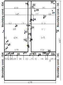
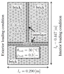
(a)	(b)

Figure 1: (a) Geometry of the masonry block with positions of sensors, (b) finite element mesh with applied loading

The experiments were conducted using the NONSTAT measuring system consisting of two climatic chambers for the simulation of climatic conditions (relative humidity, temperature), which are connected by a specially developed tunnel for testing large specimens. Although the specimen dimensions are therefore close to a real masonry structure, the accuracy of measurements remains the same as for small laboratory samples, see [15, 16] for further details. To measure temperature and moisture fields, a set of sensors was attached to the masonry specimen as seen in Fig. 1(a) with the following accuracy: capacitive relative humidity sensors are applicable in the range of humidities $0.05$-$0.98$ $\pm$ $0.02$ [-], temperature sensors provide measurements with a deviation of $\pm$ $0.4$ [${}^{\circ}\mathrm{C}$] in the temperature range from -20 to 0 [${}^{\circ}\mathrm{C}$] and $\pm$ $0.1$ [${}^{\circ}\mathrm{C}$] in the range from $0$ to $70$ [${}^{\circ}\mathrm{C}$].

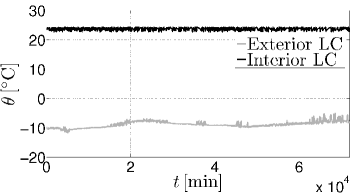
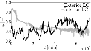
(a)	(b)

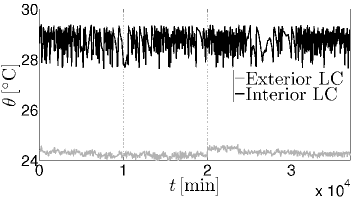
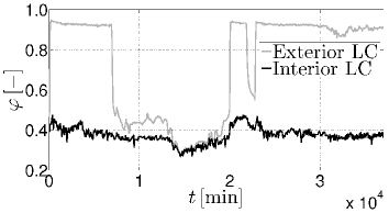
Figure 2: Experiment No. 1: Loading conditions - (a) temperature, (b) relative humidity

(a)	(b)

Figure 3: Experiment No. 2: Loading conditions - (a) temperature, (b) relative humidity

Two separate experiments were conducted. In the first experiment, the heat transport was driven by the temperature gradient, whereas the relative humidity was maintained at a constant level. In the second experiment, the relative humidity transport was monitored at approximately constant temperature. The real climatic conditions generated on both the interior and exterior part of the wall sample for the first and second experiment are displayed in Figs. 3 and 3, respectively. Notice that although expected to be constant around the value of 0.5, the relative humidity in the first experiment shows considerable fluctuations exceeding the range of 0.2 [-]. Moreover, the measurements in the second experiments were polluted by two electricity shutdowns clearly visible in Fig. 3 resulting in a severe drop of relative humidity on the exterior part of the specimen. It should, however, be mentioned that despite of that, none of these two complications in the control of relative humidity are of major concern in the identification of material parameters since the exact record of boundary conditions, with limitations to the selected time step, was introduced in all numerical calculations.

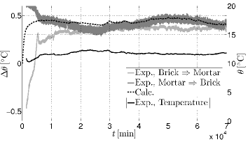
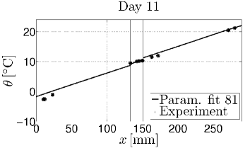
(a)	(b)

Figure 4: Experiment No. 1: (a) comparison of experimentally and numerically obtained temperature jumps along the interface, (b) calculated and measured temperature profile in chosen sensors corresponding to $11^{\mathrm{th}}$ day

3.2 Numerical simulation

The first experiment was focused on the heat transport trough the masonry block, especially in the area of interface transition zone. On the exterior side of the specimen, a constant temperature of $-9.5$ [${}^{\circ}\mathrm{C}$] and on the interior side, a constant temperature of $24.5$ [${}^{\circ}\mathrm{C}$] were maintained, see Fig. 3(a). The experimental measurement lasted $50$ days. All experiments were performed considering the moisture in the form of water vapor only. Therefore, no additional difficulties associated with ice formation in large pores aroused in numerical simulations. Nevertheless, if this issue becomes important the present model can be modified, as suggested in [11], allowing us to determine the amount of movable water for a given temperature.

Distribution of temperature in the selected points close to the interface served to extract the corresponding jumps and to assess their dependence on temperature and relative humidity on the one hand and on the other hand their sensitivity to the direction of flow. The experimentally obtained time variation of temperature jumps is plotted in Fig. 4 suggesting its invariance with respect to both temperature and flow direction, at least for the present experimental setup. An example of variation of temperature is plotted in Fig. 4(a) for sensor No. 12. Reproducing these results numerically would thus allow us to derive the respective interface heat transfer coefficient $\alpha_{\mathrm{int}}$.

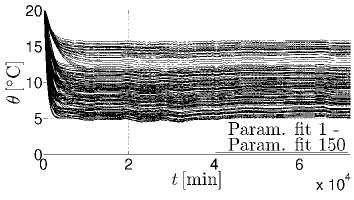
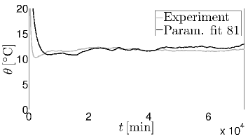
(a)	(b)

Figure 5: Experiment No. 1: (a) evolution of temperature obtained from all numerical calculations in sensor No. $12$, (b) evolution of temperature obtained numerically for optimal data and from experiment in sensor No. $12$

If material parameters of individual phases were available and assuming the relative humidity is continuous this would be the only parameter to be searched for. Unfortunately, no additional experiments were conducted for this type of material and had to be identified along with the parameter $\alpha_{\mathrm{int}}$. Although a variety of techniques, typically exploiting the power of genetic algorithms, are available in the literature, see e.g.  [17, 18], a simple ”trial and error” procedure was adopted here to mine the necessary material data. To that end, the moisture transport parameters were taken from literature for a similar type of material [2], while the remaining thermal properties of brick, mortar and interface transition zone, namely the thermal conductivity of dry building material $\lambda_{\mathrm{0}}$ [Wm^-1K^-1], the thermal conductivity supplement $b_{\mathrm{tcs}}$ [-] and the interface heat transfer coefficient $\alpha_{\mathrm{int}}$ [Wm^-2K^-1] were found by matching the experimental and numerical results in the framework of least square method applied to a pool of numerical realizations with input parameters generated by the Latin Hypercube Sampling method assuming Log-normal distribution of material data to simply avoid possibly negative values of parameters generated for individual realizations. The mean values are taken again from [2].

Geometrical model and boundary conditions used in numerical calculations appear in Fig. 1(b). The finite element mesh consisted of 662 triangular and 57 interface elements. The calculated curves entering the inverse analysis are plotted in Fig. 5(a). The results representing the temperature in the area of interface transition zone (ITZ) are displayed in Fig. 5(b). The numerically predicted temperature jumps are presented in Fig. 4(a) assuming a single value of parameter $\alpha_{\mathrm{int}}$ independent of both temperature and flow direction. The calculated and measured temperature profiles for optimally fitted thermal data are compared in Fig. 5(b).

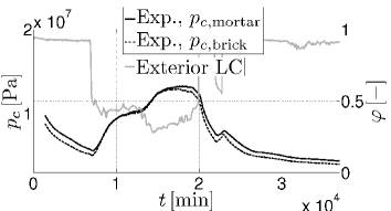
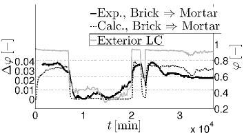
(a)	(b)

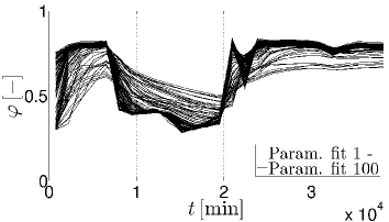
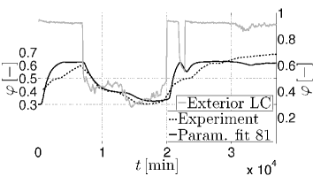
Figure 6: Experiment No. 2: (a) distribution of back calculated capillary pressures along the interface, (b) comparison of experimentally and numerically obtained relative humidity jumps along the interface

(a)	(b)

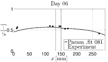
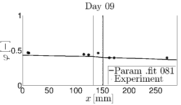
Figure 7: Experiment No. 2: (a) evolution of relative humidity obtained from all numerical calculations in sensor No. $14$, (b) evolution of relative humidity obtained numerically for optimal data and from experiment in sensor No. $14$

(a)	(b)

Figure 8: Experiment No. 2: Calculated and measured relative humidity profile in chosen sensors corresponding to: (a) $6^{\mathrm{th}}$ day, (b) $9^{\mathrm{th}}$ day

The second experiment simulated a water vapor transport within a steady state temperature profile. On the exterior side of the wall the relative humidity of 0.3 [-] and on the interior side of 0.95 [-] were prescribed, see Fig. 3. The temperature varied in the range of 25 to 29 [${}^{\circ}\mathrm{C}$]. This experiment lasted 27 days. As before independence of jumps in relative humidity with respect to the flow direction was again observed. Thus only jumps pertinent to brick-mortar transition are presented, see Fig. 8(b). Noticing that the actual values of these jumps are essentially comparable to the measuring precision may support the notion of a perfect hydraulic contact. In the next paragraphs we seek to confirm this via numerical simulations.

As for numerical calculations, a similar generation of material parameters as in the previous numerical example was carried out, see Fig. 8, to capture the necessary relative humidity input data for both material phases (free water saturation $w_{f}$ [kgm^-3], water content $w_{80}$[kgm^-3] at 0.8 [-] relative humidity, water vapor diffusion resistance factor $\mu$ [-], water absorption coefficient $A$ [kgm^-2s^-0.5] and interface permeability $\beta_{\mathrm{int}}$ [kgm^-2s^-1Pa^-1]. Again, the finite element mesh as seen in Fig. 1(b) was used with the thermal material parameters of mortar and bricks ($\left\{\lambda_{0,\mathrm{m}},\lambda_{0,\mathrm{b}}\right\}=\left\{0.45,0.25\right\}$, $\left\{b_{\mathrm{tcs,m}},b_{\mathrm{tcs,b}}\right\}=\left\{9.0,10.0\right\}$, $\alpha_{\mathrm{int}}=100000$) found from the first identification problem.

Fig. 8(a) represents a collection of all possible variations of relative humidity, while Fig. 8(b) displays the evolution of moisture for optimally fitted set of parameters ($\left\{w_{\mathrm{f,m}},w_{\mathrm{f,b}}\right\}=\left\{160.0,229.30\right\}$, $\left\{w_{80,\mathrm{m}},w_{80,\mathrm{b}}\right\}=\left\{22.72,141.68\right\}$, $\left\{\mu_{\mathrm{m}},\mu_{\mathrm{b}}\right\}=\left\{9.63,16.80\right\}$, $\left\{A_{\mathrm{m}},A_{\mathrm{b}}\right\}=\left\{0.82,0.51\right\}$, $\beta_{\mathrm{int}}=5.25\times{10}^{-9}$) derived from the ”trial and error” procedure.

The experimentally and numerically obtained results for the interface transition zone are plotted in Fig. 8 depicting distributions of capillary pressures and jumps in relative humidity in individual phases in the vicinity of the interface. Note that capillary pressures are not directly measured but arise from back calculation by introducing the corresponding values of experimentally measured relative humidities in Kelvin’s equation (7). Their discontinuous variation further supports our assumption of an imperfect hydraulic contact. As seen from both figures the experimental measurement was affected by the fault of boundary condition on the exterior side of the masonry wall due to electricity shutdown so that the identification of jumps in this time period was rather complicated and therefore, as can be seen from Fig. 8(b), the agreement between numerical and experimental estimates is less accurate. It is also worth noting that the jump magnitude in relative humidity is almost equal to the accuracy of sensors. Therefore, incorporating the interface elements into numerical calculations will probably have negligible influence on the predicted results.

The calculated moisture profile and measured relative humidity for the optimally fitted thermal and moisture material parameters are depicted in Fig. 8.

4 Homogenization on meso-scale

Once having derived the material parameters of individual phases we may now proceed to address the two principal objectives, recall the introductory part, in the light of the first order homogenization theory. To that end, we consider an RVE in terms of a periodic unit cell (PUC) describing the geometrical and material details of the meso-scale, see Fig. 9.

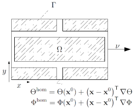
Figure 9: Periodic unit cell of brick-mortar composite with assumed boundary conditions

4.1 Fundamentals of 1st order homogenization

Since examining only the coupling effect and influence of interface transition parameters on the homogenized properties, it is sufficient to consider a steady state problem and perform a detailed parametric study on meso-scale. Because only first order homogenization is adopted, it is assumed that macroscopic temperature and relative humidity vary only linearly over the PUC. This can be achieved by loading the boundary of the PUC by the prescribed temperature $\theta^{\mathrm{hom}}$ and relative humidity $\varphi^{\mathrm{hom}}$ derived from uniform macroscopic temperature $\mbox{\boldmath$\nabla$}\Theta$ and relative humidity $\mbox{\boldmath$\nabla$}\Phi$ gradients, respectively, as depicted in Fig. 9.

In such a case, the local temperature and relative humidity admit the following decomposition

$$\theta(\mbox{\boldmath$x$}) = \Theta(\mbox{\boldmath$x$}^{0})+\left(\mbox{\boldmath$x$}-\mbox{\boldmath$x$}^{0}\right)^{\sf T}\mbox{\boldmath$\nabla$}\Theta+\theta^{*}(\mbox{\boldmath$x$})\,=\,\Theta^{\mathrm{hom}}+\theta^{*},$$

$$\varphi(\mbox{\boldmath$x$}) = \Phi(\mbox{\boldmath$x$}^{0})+\left(\mbox{\boldmath$x$}-\mbox{\boldmath$x$}^{0}\right)^{\sf T}\mbox{\boldmath$\nabla$}\Phi+\varphi^{*}(\mbox{\boldmath$x$})\,=\,\Phi^{\mathrm{hom}}+\varphi^{*},$$ (9)

where $\mbox{\boldmath$\nabla$}\Theta$ and $\mbox{\boldmath$\nabla$}\Phi$ are the macroscopically uniform temperature and relative humidity gradients, respectively. Fluctuations of local fields about the macroscopic ones are denoted by $\theta^{*}(\mbox{\boldmath$x$})$ and $\varphi^{*}(\mbox{\boldmath$x$})$. Finally, the temperature $\Theta(\mbox{\boldmath$x$}^{0})$ and the relative humidity $\Phi(\mbox{\boldmath$x$}^{0})$ at the reference point $\mbox{\boldmath$x$}^{0}$ are introduced to uniquely define the distributions of the corresponding local fields. The micro-temperature and micro-relative humidity gradients

$$\mbox{\boldmath$\nabla$}\theta(\mbox{\boldmath$x$}) = \mbox{\boldmath$\nabla$}\Theta+\mbox{\boldmath$\nabla$}\theta^{*}(\mbox{\boldmath$x$}),$$

$$\mbox{\boldmath$\nabla$}\varphi(\mbox{\boldmath$x$}) = \mbox{\boldmath$\nabla$}\Phi+\mbox{\boldmath$\nabla$}\varphi^{*}(\mbox{\boldmath$x$}),$$ (10)

averaged over the volume $|\Omega|$ of the PUC

$$\langle\mbox{\boldmath$\nabla$}\theta(\mbox{\boldmath$x$})\rangle = \frac{1}{|\Omega|}\int_{\Omega}\mbox{\boldmath$\nabla$}\theta(\mbox{\boldmath$x$})\mathrm{d}\Omega(\mbox{\boldmath$x$})=\mbox{\boldmath$\nabla$}\Theta+\frac{1}{|\Omega|}\int_{\Omega}\mbox{\boldmath$\nabla$}\theta^{*}(\mbox{\boldmath$x$})\mathrm{d}\Omega(\mbox{\boldmath$x$}),$$

$$\langle\mbox{\boldmath$\nabla$}\varphi(\mbox{\boldmath$x$})\rangle = \frac{1}{|\Omega|}\int_{\Omega}\mbox{\boldmath$\nabla$}\varphi(\mbox{\boldmath$x$})\mathrm{d}\Omega(\mbox{\boldmath$x$})=\mbox{\boldmath$\nabla$}\Phi+\frac{1}{|\Omega|}\int_{\Omega}\mbox{\boldmath$\nabla$}\varphi^{*}(\mbox{\boldmath$x$})\mathrm{d}\Omega(\mbox{\boldmath$x$}),$$ (11)

yield the scale transition relation, see e.g. [3],

$$\langle\mbox{\boldmath$\nabla$}\theta^{*}\rangle = \frac{1}{|\Omega|}\int_{\Omega}\mbox{\boldmath$\nabla$}\theta^{*}(\mbox{\boldmath$x$})\mathrm{d}\Omega(\mbox{\boldmath$x$})=\frac{1}{|\Omega|}\int_{\Gamma}\theta^{*}(\mbox{\boldmath$x$})\mbox{\boldmath$\nu$}\mathrm{d}\Gamma(\mbox{\boldmath$x$})=0,$$

$$\langle\mbox{\boldmath$\nabla$}\varphi^{*}\rangle = \frac{1}{|\Omega|}\int_{\Omega}\mbox{\boldmath$\nabla$}\varphi^{*}(\mbox{\boldmath$x$})\mathrm{d}\Omega(\mbox{\boldmath$x$})=\frac{1}{|\Omega|}\int_{\Gamma}\varphi^{*}(\mbox{\boldmath$x$})\mbox{\boldmath$\nu$}\mathrm{d}\Gamma(\mbox{\boldmath$x$})=0.$$ (12)

The boundary integral disappears providing either the fluctuation parts of the local fields equal zero (Dirichlet boundary conditions) or the periodic boundary conditions, i.e. the same values of $\theta^{*}$ and $\varphi^{*}$ on opposite sides of the rectangular PUC, are enforced on $\Gamma$.

4.2 Discretized form of energy balance equation

Using Eqs. (1) and (3) the heat flux density is given by

$$\mbox{\boldmath$q$}+h_{v}\mbox{\boldmath$g$}_{v} = -\lambda\mbox{\boldmath$\nabla$}\theta-h_{v}\delta_{p}\mbox{\boldmath$\nabla$}(\varphi p_{\mathrm{sat}})$$ (13)

$$= -\lambda\mbox{\boldmath$\nabla$}\theta-h_{v}\delta_{p}p_{\mathrm{sat}}\mbox{\boldmath$\nabla$}\varphi-h_{v}\delta_{p}\varphi\mbox{\boldmath$\nabla$}p_{\mathrm{sat}}.$$

Next, substituting for local fields $\theta$ and $\varphi$ from Eq. (10) into (13) and after some manipulations we get

$$\mbox{\boldmath$q$}+h_{v}\mbox{\boldmath$g$}_{v}=-[\lambda+h_{v}\delta_{p}\frac{\mathrm{d}p_{\mathrm{sat}}}{\mathrm{d}\theta}\varphi](\mbox{\boldmath$\nabla$}\Theta+\mbox{\boldmath$\nabla$}\theta^{*})-h_{v}\delta_{p}p_{\mathrm{sat}}(\mbox{\boldmath$\nabla$}\Phi+\mbox{\boldmath$\nabla$}\varphi^{*}).$$ (14)

The stepping stone in the estimation of macroscopic response is the Hill-Mandel lemma suggesting equality of the work of local fields averaged over the solution domain and the work of their macroscopic counterparts. Owing to the nonlinear nature of underlying material models, the formulation must be written in an incremental form. To that end, assume an equilibrium state at the end of the $i$-th time step and consider a small increment of the macroscopic temperature gradient $\mathrm{d}(\mbox{\boldmath$\nabla$}\Theta)$ resulting in an incremental change of local and macroscopic fluxes so that

$$\left\langle-\delta(\mbox{\boldmath$\nabla$}\theta){\sf{}^{T}}\mathrm{d}(\mbox{\boldmath$q$}+h_{v}\mbox{\boldmath$g$}_{v})\right\rangle=-\delta(\mbox{\boldmath$\nabla$}\Theta){\sf{}^{T}}\mathrm{d}(\mbox{\boldmath$q$}^{\mathrm{M}}+h_{v}^{\mathrm{M}}\mbox{\boldmath$g$}_{v}^{\mathrm{M}}),$$ (15)

where the symbol $\langle\cdot\rangle=\frac{1}{|\Omega|}\int_{\Omega}\cdot\mathrm{d}\Omega$ represents the volume averaging. Providing we admit only the Dirichlet boundary conditions in the form of the prescribed gradient of macroscopic temperature the term on the right hand side would disappear ($\delta(\mbox{\boldmath$\nabla$}\Theta)=\mbox{\boldmath$0$}$). For the calculation purposes this condition is considered to determine the unknown fluctuation fields. Nevertheless, for the derivation of instantaneous macroscopic conductivity matrix it will prove useful to keep the full generality of the mathematical formulation.

To proceed, consider the numerical solution in the framework of the finite element method and introduce the standard geometric matrix $\mathsf{B}$ storing the spatial derivatives of the finite element shape functions to get the discretized form of the local fields as

$$\mbox{\boldmath$\nabla$}\theta=\mbox{\boldmath$\nabla$}\Theta+\mbox{\boldmath$\mathsf{B}$}\mbox{\boldmath$r$}_{\theta}^{*},\qquad\mbox{\boldmath$\nabla$}\varphi=\mbox{\boldmath$\nabla$}\Phi+\mbox{\boldmath$\mathsf{B}$}\mbox{\boldmath$r$}_{\varphi}^{*},$$ (16)

and

$$\delta(\mbox{\boldmath$\nabla$}\theta)=\delta(\mbox{\boldmath$\nabla$}\Theta)+\mbox{\boldmath$\mathsf{B}$}\delta\mbox{\boldmath$r$}_{\theta}^{*},\qquad\delta(\mbox{\boldmath$\nabla$}\varphi)=\delta(\mbox{\boldmath$\nabla$}\Phi)+\mbox{\boldmath$\mathsf{B}$}\delta\mbox{\boldmath$r$}_{\varphi}^{*}.$$ (17)

Substituting Eqs. (14), (16) and (17) into Eq. (15) provides

$$\delta(\mbox{\boldmath$\nabla$}\Theta){\sf{}^{T}}\{\mathrm{d}(\mbox{\boldmath$q$}^{\mathrm{M}}+h_{v}^{\mathrm{M}}\mbox{\boldmath$g$}_{v}^{\mathrm{M}})+$$

$$\qquad+\underbrace{\left\langle\lambda+h_{v}\delta_{p}\frac{\mathrm{d}p_{\mathrm{sat}}}{\mathrm{d}\theta}\hat{\Phi}^{\mathrm{hom}}\right\rangle}_{\mbox{\boldmath$\mathsf{K}$}_{\theta\theta}^{\mathrm{m}}}\mathrm{d}(\mbox{\boldmath$\nabla$}\Theta)+\underbrace{\left\langle h_{v}\delta_{p}p_{\mathrm{sat}}\right\rangle}_{\mbox{\boldmath$\mathsf{K}$}_{\theta\varphi}^{\mathrm{m}}}\mathrm{d}(\mbox{\boldmath$\nabla$}\Phi)+$$

$$\qquad+\underbrace{\left\langle[\lambda+h_{v}\delta_{p}\frac{\mathrm{d}p_{\mathrm{sat}}}{\mathrm{d}\theta}\hat{\Phi}^{\mathrm{hom}}]\mbox{\boldmath$\mathsf{B}$}\right\rangle}_{\mbox{\boldmath$\mathsf{L}$}_{\theta\theta}}\mathrm{d}\mbox{\boldmath$r$}_{\theta}^{*}+\underbrace{\left\langle h_{v}\delta_{p}p_{\mathrm{sat}}\mbox{\boldmath$\mathsf{B}$}\right\rangle}_{\mbox{\boldmath$\mathsf{L}$}_{\theta\varphi}}\mathrm{d}\mbox{\boldmath$r$}_{\varphi}^{*}\}+$$

$$+\delta(\mbox{\boldmath$r$}_{\theta}^{*}){\sf{}^{T}}\{\underbrace{\left\langle\mbox{\boldmath$\mathsf{B}$}^{\sf T}[\lambda+h_{v}\delta_{p}\frac{\mathrm{d}p_{\mathrm{sat}}}{\mathrm{d}\theta}\hat{\Phi}^{\mathrm{hom}}]\right\rangle}_{\mbox{\boldmath$\mathsf{L}$}_{\theta\theta}^{\sf T}}\mathrm{d}(\mbox{\boldmath$\nabla$}\Theta)+\underbrace{\left\langle\mbox{\boldmath$\mathsf{B}$}^{\sf T}h_{v}\delta_{p}p_{\mathrm{sat}}\right\rangle}_{\mbox{\boldmath$\mathsf{L}$}_{\theta\varphi}^{\sf T}}\mathrm{d}(\mbox{\boldmath$\nabla$}\Phi)+$$

$$\qquad+\underbrace{\left\langle\mbox{\boldmath$\mathsf{B}$}^{\sf T}[\lambda+h_{v}\delta_{p}\frac{\mathrm{d}p_{\mathrm{sat}}}{\mathrm{d}\theta}\hat{\Phi}^{\mathrm{hom}}]\mbox{\boldmath$\mathsf{B}$}\right\rangle}_{\mbox{\boldmath$\mathsf{K}$}_{\theta\theta}}\mathrm{d}\mbox{\boldmath$r$}_{\theta}^{*}+\underbrace{\left\langle\mbox{\boldmath$\mathsf{B}$}{\sf{}^{T}}h_{v}\delta_{p}p_{\mathrm{sat}}\mbox{\boldmath$\mathsf{B}$}\right\rangle}_{\mbox{\boldmath$\mathsf{K}$}_{\theta\varphi}}\mathrm{d}\mbox{\boldmath$r$}_{\varphi}^{*}\}=0,$$ (18)

where the notation $\hat{\Phi}^{\mathrm{hom}}={\Phi}^{\mathrm{hom}}+\hat{\varphi}^{*}$ is introduced to identify $\hat{\varphi}^{*}$ with the fluctuation of relative humidity at the end of the previous iteration step. Because of the independence of variations $\delta(\mbox{\boldmath$\nabla$}\Theta)$ and $\delta\mbox{\boldmath$r$}_{\theta}^{*}$, Eq. (18) splits into two equalities. Noting that the change of the macroscopic flux can be expressed in the form

$$\mathrm{d}(\mbox{\boldmath$q$}^{\mathrm{M}}+h_{v}^{\mathrm{M}}\mathrm{d}\mbox{\boldmath$g$}_{v}^{\mathrm{M}})=-\mbox{\boldmath$\mathsf{K}$}_{\theta\theta}^{\mathrm{M}}\mathrm{d}(\mbox{\boldmath$\nabla$}\Theta)-\mbox{\boldmath$\mathsf{K}$}_{\theta\varphi}^{\mathrm{M}}\mathrm{d}(\mbox{\boldmath$\nabla$}\Phi),$$ (19)

we write the first equality as

$$(-\mbox{\boldmath$\mathsf{K}$}_{\theta\theta}^{\mathrm{M}}+\mbox{\boldmath$\mathsf{K}$}_{\theta\theta}^{\mathrm{m}})\mathrm{d}(\mbox{\boldmath$\nabla$}\Theta)+(-\mbox{\boldmath$\mathsf{K}$}_{\theta\varphi}^{\mathrm{M}}+\mbox{\boldmath$\mathsf{K}$}_{\theta\varphi}^{\mathrm{m}})\mathrm{d}(\mbox{\boldmath$\nabla$}\Phi)+\mbox{\boldmath$\mathsf{L}$}_{\theta\theta}\mathrm{d}\mbox{\boldmath$r$}_{\theta}^{*}+\mbox{\boldmath$\mathsf{L}$}_{\theta\varphi}\mathrm{d}\mbox{\boldmath$r$}_{\varphi}^{*}=0.$$ (20)

The second equality is then provided by

$$\mbox{\boldmath$\mathsf{L}$}_{\theta\theta}^{\sf T}\mathrm{d}(\mbox{\boldmath$\nabla$}\Theta)+\mbox{\boldmath$\mathsf{L}$}_{\theta\varphi}^{\sf T}\mathrm{d}(\mbox{\boldmath$\nabla$}\Phi)+\mbox{\boldmath$\mathsf{K}$}_{\theta\theta}\mathrm{d}\mbox{\boldmath$r$}_{\theta}^{*}+\mbox{\boldmath$\mathsf{K}$}_{\theta\varphi}\mathrm{d}\mbox{\boldmath$r$}_{\Phi}^{*}=0.$$ (21)

4.3 Discretized form of mass balance equation

Similar to Eq. (15)) the variational form of the Hill-Mandel lemma for moisture transport reads

$$\left\langle-\delta(\mbox{\boldmath$\nabla$}\varphi){\sf{}^{T}}[\mathrm{d}(\mbox{\boldmath$g$}_{v}+\mbox{\boldmath$g$}_{w})]\right\rangle=-\delta(\mbox{\boldmath$\nabla$}\Phi)^{\sf T}[\mbox{\boldmath$g$}_{v}^{\mathrm{M}}\mathrm{d}(\mbox{\boldmath$g$}_{v}^{\mathrm{M}}+\mbox{\boldmath$g$}_{w}^{\mathrm{M}})],$$ (22)

where the moisture flux density is given by

$$\mbox{\boldmath$g$}_{v}+\mbox{\boldmath$g$}_{w}=-(D_{\varphi}+\delta_{p}p_{\mathrm{sat}})(\mbox{\boldmath$\nabla$}\Phi+\mbox{\boldmath$\nabla$}\varphi^{*})-\delta_{p}\frac{\mathrm{d}p_{\mathrm{sat}}}{\mathrm{d}\theta}\varphi(\mbox{\boldmath$\nabla$}\Theta+\mbox{\boldmath$\nabla$}\theta^{*}).$$ (23)

Introducing Eq. (23) together with Eqs. (16) and (17) into Eq. (22) yields

$$\delta(\mbox{\boldmath$\nabla$}\Phi){\sf{}^{T}}\{\mathrm{d}(\mbox{\boldmath$g$}_{v}^{\mathrm{M}}+\mbox{\boldmath$g$}_{w}^{\mathrm{M}})+$$

$$\qquad+\underbrace{\left\langle\delta_{p}\frac{\mathrm{d}p_{\mathrm{sat}}}{\mathrm{d}\theta}\hat{\Phi}^{\mathrm{hom}}\right\rangle}_{\mbox{\boldmath$\mathsf{K}$}_{\varphi\theta}^{\mathrm{m}}}\mathrm{d}(\mbox{\boldmath$\nabla$}\Theta)+\underbrace{\left\langle D_{\varphi}+\delta_{p}p_{\mathrm{sat}}\right\rangle}_{\mbox{\boldmath$\mathsf{K}$}_{\varphi\varphi}^{\mathrm{m}}}\mathrm{d}(\nabla\Phi)+$$

$$\qquad+\underbrace{\left\langle[\delta_{p}\frac{\mathrm{d}p_{\mathrm{sat}}}{\mathrm{d}\theta}\hat{\Phi}^{\mathrm{hom}}]\mbox{\boldmath$\mathsf{B}$}\right\rangle}_{\mbox{\boldmath$\mathsf{L}$}_{\varphi\theta}}\mathrm{d}\mbox{\boldmath$r$}_{\theta}^{*}+\underbrace{\left\langle[D_{\varphi}+\delta_{p}p_{\mathrm{sat}}]\mbox{\boldmath$\mathsf{B}$}\right\rangle}_{\mbox{\boldmath$\mathsf{L}$}_{\varphi\varphi}}\mathrm{d}\mbox{\boldmath$r$}_{\varphi}^{*}\}+$$

$$+\delta(\mbox{\boldmath$r$}_{\varphi}^{*}){\sf{}^{T}}\{\underbrace{\left\langle\mbox{\boldmath$\mathsf{B}$}^{\sf T}[\delta_{p}\frac{\mathrm{d}p_{\mathrm{sat}}}{\mathrm{d}\theta}\hat{\Phi}^{\mathrm{hom}}]\right\rangle}_{\mbox{\boldmath$\mathsf{L}$}_{\varphi\theta}^{\sf T}}\mathrm{d}(\mbox{\boldmath$\nabla$}\Theta)+\underbrace{\left\langle\mbox{\boldmath$\mathsf{B}$}^{\sf T}[D_{\varphi}+\delta_{p}p_{\mathrm{sat}}]\right\rangle}_{\mbox{\boldmath$\mathsf{L}$}_{\varphi\varphi}^{\sf T}}\mathrm{d}(\mbox{\boldmath$\nabla$}\Phi)+$$

$$\qquad+\underbrace{\left\langle\mbox{\boldmath$\mathsf{B}$}^{\sf T}[\delta_{p}\frac{\mathrm{d}p_{\mathrm{sat}}}{\mathrm{d}\theta}\hat{\Phi}^{\mathrm{hom}}]\mbox{\boldmath$\mathsf{B}$}\right\rangle}_{\mbox{\boldmath$\mathsf{K}$}_{\varphi\theta}}\mathrm{d}\mbox{\boldmath$r$}_{\theta}^{*}+\underbrace{\left\langle\mbox{\boldmath$\mathsf{B}$}^{\sf T}[D_{\varphi}+\mbox{\boldmath$\mathsf{\delta}$}_{p}p_{\mathrm{sat}}]\mbox{\boldmath$\mathsf{B}$}\right\rangle}_{\mbox{\boldmath$\mathsf{K}$}_{\varphi\varphi}}\mathrm{d}\mbox{\boldmath$r$}_{\varphi}^{*}\}=0.$$ (24)

Since (compare with (19))

$$\mathrm{d}(\mbox{\boldmath$g$}_{v}^{\mathrm{M}}+\mbox{\boldmath$g$}_{w}^{\mathrm{M}})=-\mbox{\boldmath$\mathsf{K}$}_{\varphi\theta}^{\mathrm{M}}\mathrm{d}(\mbox{\boldmath$\nabla$}\Theta)-\mbox{\boldmath$\mathsf{K}$}_{\varphi\varphi}^{\mathrm{M}}\mathrm{d}(\mbox{\boldmath$\nabla$}\Phi),$$ (25)

the Hill-Mandel lemma for moisture transport (compare with Eq. (20)) becomes

$$(-\mbox{\boldmath$\mathsf{K}$}_{\varphi\theta}^{\mathrm{M}}+\mbox{\boldmath$\mathsf{K}$}_{\varphi\theta}^{\mathrm{m}})\mathrm{d}(\mbox{\boldmath$\nabla$}\Theta)+(-\mbox{\boldmath$\mathsf{K}$}_{\varphi\varphi}^{\mathrm{M}}+\mbox{\boldmath$\mathsf{K}$}_{\varphi\varphi}^{\mathrm{m}})\mathrm{d}(\mbox{\boldmath$\nabla$}\Phi)+\mbox{\boldmath$\mathsf{L}$}_{\varphi\theta}\mathrm{d}\mbox{\boldmath$r$}_{\theta}^{*}+\mbox{\boldmath$\mathsf{L}$}_{\varphi\varphi}\mathrm{d}\mbox{\boldmath$r$}_{\varphi}^{*}=0,$$ (26)

together with (recall Eg. (21))

$$\mbox{\boldmath$\mathsf{L}$}_{\varphi\theta}^{\sf T}\mathrm{d}(\mbox{\boldmath$\nabla$}\Theta)+\mbox{\boldmath$\mathsf{L}$}_{\varphi\varphi}^{\sf T}\mathrm{d}(\mbox{\boldmath$\nabla$}\Phi)+\mbox{\boldmath$\mathsf{K}$}_{\varphi\theta}\mathrm{d}\mbox{\boldmath$r$}_{\theta}^{*}+\mbox{\boldmath$\mathsf{K}$}_{\varphi\varphi}\mathrm{d}\mbox{\boldmath$r$}_{\varphi}^{*}=0.$$ (27)

4.4 Macroscopic conductivity matrices

Assuming that the heat and moisture balance is reached at the end of the $i$-th step at the mesostructural level and the nodal unbalanced forces are equal to zero, we obtain from the system of equations (21) and (27)

$$\left\{\begin{array}[]{c}\mathrm{d}\mbox{\boldmath$r$}_{\theta}^{*}\\ \mathrm{d}\mbox{\boldmath$r$}_{\varphi}^{*}\end{array}\right\}=-\left[\begin{array}[]{cc}\mbox{\boldmath$\mathsf{K}$}_{\theta\theta}&\mbox{\boldmath$\mathsf{K}$}_{\theta\varphi}\\ \mbox{\boldmath$\mathsf{K}$}_{\varphi\theta}&\mbox{\boldmath$\mathsf{K}$}_{\varphi\varphi}\end{array}\right]^{-1}\left[\begin{array}[]{cc}\mbox{\boldmath$\mathsf{L}$}_{\theta\theta}^{\sf T}&\mbox{\boldmath$\mathsf{L}$}_{\theta\varphi}^{\sf T}\\ \mbox{\boldmath$\mathsf{L}$}_{\varphi\theta}^{\sf T}&\mbox{\boldmath$\mathsf{L}$}_{\varphi\varphi}^{\sf T}\end{array}\right]\left\{\begin{array}[]{c}\mathrm{d}(\mbox{\boldmath$\nabla$}\Theta)\\ \mathrm{d}(\mbox{\boldmath$\nabla$}\Phi)\end{array}\right\}.$$ (28)

The system of equations (20) and (22) can be rewritten with help of Eq. (28) as

$$\left[\begin{array}[]{cc}\mbox{\boldmath$\mathsf{K}$}_{\theta\theta}^{\mathrm{M}}&\mbox{\boldmath$\mathsf{K}$}_{\theta\varphi}^{\mathrm{M}}\\ \mbox{\boldmath$\mathsf{K}$}_{\varphi\theta}^{\mathrm{M}}&\mbox{\boldmath$\mathsf{K}$}_{\varphi\varphi}^{\mathrm{M}}\end{array}\right]\left\{\begin{array}[]{c}\mathrm{d}(\mbox{\boldmath$\nabla$}\Theta)\\ \mathrm{d}(\mbox{\boldmath$\nabla$}\Phi)\end{array}\right\}=$$ (33)

$$=\left(\left[\begin{array}[]{cc}\mbox{\boldmath$\mathsf{K}$}_{\theta\theta}^{\mathrm{m}}&\mbox{\boldmath$\mathsf{K}$}_{\theta\varphi}^{\mathrm{m}}\\ \mbox{\boldmath$\mathsf{K}$}_{\varphi\theta}^{\mathrm{m}}&\mbox{\boldmath$\mathsf{K}$}_{\varphi\varphi}^{\mathrm{m}}\end{array}\right]-\left[\begin{array}[]{cc}\mbox{\boldmath$\mathsf{L}$}_{\theta\theta}&\mbox{\boldmath$\mathsf{L}$}_{\theta\varphi}\\ \mbox{\boldmath$\mathsf{L}$}_{\varphi\theta}&\mbox{\boldmath$\mathsf{L}$}_{\varphi\varphi}\end{array}\right]\left[\begin{array}[]{cc}\mbox{\boldmath$\mathsf{K}$}_{\theta\theta}&\mbox{\boldmath$\mathsf{K}$}_{\theta\varphi}\\ \mbox{\boldmath$\mathsf{K}$}_{\varphi\theta}&\mbox{\boldmath$\mathsf{K}$}_{\varphi\varphi}\end{array}\right]^{-1}\left[\begin{array}[]{cc}\mbox{\boldmath$\mathsf{L}$}_{\theta\theta}^{\sf T}&\mbox{\boldmath$\mathsf{L}$}_{\theta\varphi}^{\sf T}\\ \mbox{\boldmath$\mathsf{L}$}_{\varphi\theta}^{\sf T}&\mbox{\boldmath$\mathsf{L}$}_{\varphi\varphi}^{\sf T}\end{array}\right]\right)\left\{\begin{array}[]{c}\mathrm{d}(\mbox{\boldmath$\nabla$}\Theta)\\ \mathrm{d}(\mbox{\boldmath$\nabla$}\Phi)\end{array}\right\},$$ (44)

to finally arrive at the macroscopic conductivity matrix in the form

$$\left[\begin{array}[]{cc}\mbox{\boldmath$\mathsf{K}$}_{\theta\theta}^{\mathrm{M}}&\mbox{\boldmath$\mathsf{K}$}_{\theta\varphi}^{\mathrm{M}}\\ \mbox{\boldmath$\mathsf{K}$}_{\varphi\theta}^{\mathrm{M}}&\mbox{\boldmath$\mathsf{K}$}_{\varphi\varphi}^{\mathrm{M}}\end{array}\right]=\left[\begin{array}[]{cc}\mbox{\boldmath$\mathsf{K}$}_{\theta\theta}^{\mathrm{m}}&\mbox{\boldmath$\mathsf{K}$}_{\theta\varphi}^{\mathrm{m}}\\ \mbox{\boldmath$\mathsf{K}$}_{\varphi\theta}^{\mathrm{m}}&\mbox{\boldmath$\mathsf{K}$}_{\varphi\varphi}^{\mathrm{m}}\end{array}\right]-\left[\begin{array}[]{cc}\mbox{\boldmath$\mathsf{L}$}_{\theta\theta}&\mbox{\boldmath$\mathsf{L}$}_{\theta\varphi}\\ \mbox{\boldmath$\mathsf{L}$}_{\varphi\theta}&\mbox{\boldmath$\mathsf{L}$}_{\varphi\varphi}\end{array}\right]\left[\begin{array}[]{cc}\mbox{\boldmath$\mathsf{K}$}_{\theta\theta}&\mbox{\boldmath$\mathsf{K}$}_{\theta\varphi}\\ \mbox{\boldmath$\mathsf{K}$}_{\varphi\theta}&\mbox{\boldmath$\mathsf{K}$}_{\varphi\varphi}\end{array}\right]^{-1}\left[\begin{array}[]{cc}\mbox{\boldmath$\mathsf{L}$}_{\theta\theta}^{\sf T}&\mbox{\boldmath$\mathsf{L}$}_{\theta\varphi}^{\sf T}\\ \mbox{\boldmath$\mathsf{L}$}_{\varphi\theta}^{\sf T}&\mbox{\boldmath$\mathsf{L}$}_{\varphi\varphi}^{\sf T}\end{array}\right].$$ (45)

4.5 Numerical results

Recall the introductory part posting two particular issues to be investigated. First, we were interested in assessing the influence of interface transition parameters on the homogenized response. For this purpose, the PUC displayed in Fig. 9 was loaded by a set of prescribed macroscopic temperature $\mbox{\boldmath$\nabla$}\Theta$ and relative humidity $\mbox{\boldmath$\nabla$}\Phi$ gradients. The initial values of temperature and relative humidity were set equal to $\Theta(\mbox{\boldmath$x$}^{0})=20$ [${}^{\circ}\mathrm{C}$] and $\Phi(\mbox{\boldmath$x$}^{0})=0.5$ [-], respectively. The model parameters were found using equations listed in [12] together with phase material data derived in Section 3. To see the sensitivity of the homogenized properties on interface parameters, we assumed a set of constant values of parameters $\alpha_{\mathrm{int}}$ and $\beta_{\mathrm{int}}$ slightly varying about the optimal ones $\alpha_{\mathrm{int}}=10^{5}$ [Wm^-2K^-1] and $\beta_{\mathrm{int}}=5.25\times{10}^{-9}$ [kgm^-2s^-1Pa^-1].

The results are plotted in Fig. 10 showing variation of the selected diagonal terms of the homogenized conductivity matrix, recall Eq. (45). Clearly, while we may notice dependence of homogenized terms on macroscopic gradients, the impact of variation of $\alpha_{\mathrm{int}}$ and $\beta_{\mathrm{int}}$ is almost imperceptible. These results together with experimental observations presented in Section 3 may suggest that the introduction of interface transition zone at the mesostructural level is essentially negligible for the prediction of effective properties, at least for the present material system and applied range of temperatures and relative humidities.

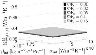
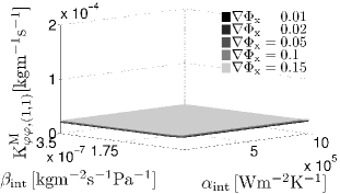
(a)	(b)

Figure 10: Variation of the effective parameters ($\mathrm{K}_{\theta\theta,(1,1)}^{\mathrm{M}}$ and $\mathrm{K}_{\varphi\varphi,(1,1)}^{\mathrm{M}}$) as a function of the interface transfer coefficients for various values of relative humidity gradients

Second, to capture the influence of macroscopic loading conditions on effective parameters we assumed, in view of the previous results, a perfect hydraulic contact and loaded the PUC again by several different macroscopic temperature and relative humidity gradients. In addition, the macroscopic/initial temperature and macroscopic/initial relative humidity also varied.

The distributions of the same macroscopic terms as in the first example appear in Fig. 11. It is evident that the predicted effective parameters are considerably dependent on both the initial and loading conditions. Despite it, one may suggest that homogenization analysis performed for various values of water content $w$ and certain referenced initial values of temperature and relative humidity can be exploited to construct the homogenized macro-scale retention curves providing the analysis is independent of the applied macroscopic gradients. Such curves would be then used in an independent macroscopic study. While this seems acceptable for effective thermal conductivities, this approach evidently fails for effective moisture transport coefficients, which strongly depend on the current temperature and relative humidity gradients. Therefore, studying the coupled heat and moisture transport in masonry structures must be envisioned in a full-fledged coupled multi-scale framework (FE² problem). On the other hand, this offers the possibility of including the mesostructural morphology and mesostructural material behavior in the macro-level, where typical structures are analyzed, without the need for assigning the fine-scale details to the entire structure.

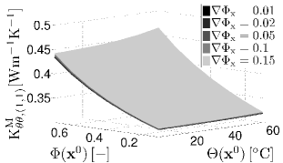
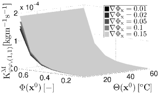
(a)	(b)

Figure 11: Variation of the effective parameters ($\mathrm{K}_{\theta\theta,(1,1)}^{\mathrm{M}}$ and $\mathrm{K}_{\varphi\varphi,(1,1)}^{\mathrm{M}}$) as a function of initial conditions for various values of relative humidity gradients

5 Conclusions

A coupled heat and moisture transport was studied with reference to the first order homogenization of masonry walls. First, a specific experimental program was executed to infer the local phase material parameters and interface transition coefficients from experimentally observed jumps in temperature and relative humidity fields. The notion of a negligible effect of considering an imperfect hydraulic contact put forward already by experimental results was further supported numerically by a parametric meso-scale homogenization study of a stationary problem.

Admitting only a perfect hydraulic contact proves useful in the light of the second set of results promoting the need for fully coupled multi-scale analysis when transport of moisture becomes appreciable, such as the case of historic masonry structures, especially bridges.

References

- [1] J. Novák, J. Zeman, M. Šejnoha, J. Šejnoha, Pragmatic multi-scale and multi-physics analysis of Charles Bridge in Prague, Engineering Structures 30 (11) (2008) 3365–3376.
- [2] J. Sýkora, J. Vorel, T. Krejčí, M. Šejnoha, J. Šejnoha, Analysis of coupled heat and moisture transfer in masonry structures, Materials and Structures 42 (8) (2009) 1153–1167.
- [3] I. Özdemir, W. Brekelmans, M. Geers, Computational homogenization for heat conduction in heterogeneous solids, International Journal for Numerical Methods in Engineering 73 (2008) 185–204.
- [4] I. Özdemir, W. Brekelmans, M. Geers, Fe2 computational homogenization for the thermo-mechanical analysis of heterogeneous solids, Computer Methods in Applied Mechanics and Engineering 198 (3-4) (2008) 602–613.
- [5] F. Larsson, K. Runesson, F. Su, Variationally consistent computational homogenization of transient heat flow, International Journal for Numerical Methods in Engineering 81 (2010) 1659–1686.
- [6] F. Larsson, K. Runesson, F. Su, Computational homogenization of uncoupled consolidation in micro-heterogeneous porous media, International Journal for Numerical and Analytical Methods in Geomechan 34 (2010) 1431–1458.
- [7] S. Lee, V. Sundararaghavan, Multi-scale homogenization of moving interface problems with flux jumps: applications to solidification, Computational mechanics 44 (2009) 297–307.
- [8] V. P. De Freitas, V. Abrantes, P. Crausse, Moisture migration in building walls - analysis of the interface phenomena, Building and Enviroment 31 (2) (1996) 99–108.
- [9] X. Qiu, F. Haghighat, M. Kumaran, Moisture transport across interfaces between autoclaved aerated concrete and mortar, Journal of Thermal Envelope & Building Science 26 (3) (2003) 213–236.
- [10] R. Černý, P. Rovnaníková, Transport Processes in Concrete, London: Spon Press, 2002.
- [11] H. M. Künzel, Simultaneous Heat and Moisture Transport in Building Components, Tech. rep., Fraunhofer IRB Verlag Stuttgart (1995).
- [12] H. Künzel, K. Kiessl, Calculation of heat and moisture transfer in exposed building components, International Journal of Heat Mass Transfer 40 (1997) 159–167.
- [13] J. C. Michel, H. Moulinec, P. Suquet, Effective properties of composite materials with periodic microstructure: A computational approach, Computer Methods in Applied Mechanics and Engineering 172 (1999) 109–143.
- [14] J. Šejnoha, M. Šejnoha, J. Zeman, J. Sýkora, J. Vorel, Mesoscopic study on historic masonry, Structural Engineering and Mechanics 30 (1) (2008) 99–117.
- [15] Z. Pavlík, J. Pavlík, M. Jiřičková, R. Černý, System for testing the hygrothermal performance of multi-layered building envelopes, Journal of Thermal Envelope and Building Science 25 (2002) 239–249.
- [16] Z. Pavlík, J. Mihulka, J. Žumár, R. Černý, Experimental monitoring of moisture transfer across interfaces in brick masonry, in: Structural Faults and Repair, 2010.
- [17] K. Matouš, M. Lepš, J. Zeman, M. Šejnoha, Applying genetic algorithms to selected topics commonly encountered in engineering practice, Computer Methods in Applied Mechanics and Engineering 190 (13–14) (2000) 1629–1650.
- [18] A. Kučerová, Identification of nonlinear mechanical model parameters based on softcomputing methods, Ph.D. thesis, Ecole Normale Supérieure de Cachan, Laboratoire de Mécanique et Technologie (2007).