Correlated valence bond state and its study of the spin-$1/2$ $J_{1}-J_{2}$ Antiferromagnetic Heisenberg model on a square lattice

Abstract

We propose a class of variational wavefunctions, namely the correlated valence bond states, for the frustrated Hamiltonians in the paramagnetic phase. This class of wavefunctions admits negative amplitude and the same sublattice pairing when a bipartite lattice is considered, thus suffers from the negative sign problem. However if applied to small systems, the sign problem is manageable using the standard variational Monte Carlo method. We optimize the wavefunctions for the $J_{1}-J_{2}$ Antiferromagnetic Heisenberg model on a square lattice in the coupling region $J_{2}/J_{1}\in[0.45:0.56]$ for system sizes $L=4,6,8$. To calculate the correlation functions and the order parameters for larger systems, we make the extensive Monte Carlo samplings using the variational parameters optimized at system size $L=8$. We find that the paramagnetic phase is a gapless spin liquid in the entire range of $J_{2}/J_{1}\in[0.45:0.56]$ with a gapless singlet excitation and a gaped triplet excitation.

I Introduction

The $J_{1}-J_{2}$ antiferromagnetic (AF) Heisenberg model on a square lattice has attracted a lot of attention due to its close relation to the disappearance of the AF order in high-T_c superconducting material anderson1 ; anderson2 ; Inui ; lyons ; wen_review_hightc and its possibility of realizing the so called spin liquid state chandra88 ; ed2 ; ed4 ; Capriotti_prl87.097201 ; richter_ed ; tao ; ling ; jiang ; huwenjun . The spin liquids, defined as lacking long range order and supporting strong quantum fluctuation, have all the key properties of the insulating state “nearby” to a superconducting phase. Hence a simple example of spin liquids, the resonating valence bond (RVB) state was proposed to describe high-T_c superconductivity anderson1 ; anderson2 . Spin liquids have become the focus of research in modern condensed matter physics since the discovery of different kinds of spin liquids in theory KL8795 ; WWZ8913 ; RS9173 ; W9164 ; SondhiZ2 ; HongZ2 . Although the existence and stability of spin liquids in realistic models and real material are still in question kagomeSL ; stefan ; spinliquid1 ; spinliquid2 ; spinliquid3 .

The nature of the ground state of the $J_{1}-J_{2}$ AF Heisenberg model in the intermediate coupling region has been debated gelfand89 ; chubukov91 ; chandra88 ; chandra90 ; subir ; WWZ8913 ; W9164 ; ed1 ; ed2 ; ed3 ; ed4 ; ed5 ; richter_ed ; sirker_prb73.184420 ; darradi_prb78.214415 ; kevin_prb79.224431 ; mambrini_prb74.144422 ; arlego_prb78.224415 ; Capriotti_prl87.097201 ; Capriotti_prl84.3173 ; valentin ; tao ; ling for decades due to the highly frustrated nature of this model and is still a open question. Recently, several numerical works revisited this model using novel concept, such as the topological entanglement entropy (TEE) jiang , and new numerical tools, such as the projected entangled pair states (PEPSs) valentin ; ling . Amazingly many of them have reached a consistent and the lowest ground state energy ever huwenjun ; jiang ; gong ; ling , however their resulting ground states behave diversely. A density matrix renormalization group (DMRG) study on long cylinders suggested a gaped $\mathbb{Z}_{2}$ spin liquids from the evidences of non-vanishing singlet and triplet gaps in the paramagnetic phase and a nonzero TEE jiang . The Gutzwiller-projected BCS wavefunction study indicated a gapless spin liquid state supported by the existence of gapless triplet excitations at momenta $(\pi,0)$ and $(0,\pi)$ huwenjun . Most recently, the DMRG study with $\text{SU}(2)$ symmetry imposed on the states on long cylinders found a diverging dimer correlation length, and claimed a plaquette valence bond solid (VBS) state as the ground state gong . These controversial results pose the question about the numerical convergence and the system size dependence anders2 .

In this paper, we propose a novel wavefunction and use the variational Monte Carlo (VMC) method to tackle this system. As one knows, the key to a meaningful variational method is to have a good trial wavefunction. Here, we take a resonating valence bond state approach. The reasons for such a choice are the following, first of all, RVB states can describe a variety of phases including the spin liquids, the AF long range ordered states and the valence bond solids KL8795 ; SondhiZ2 ; HongZ2 ; didier1 ; albuquerque ; tang ; kevin2 ; jie1 ; lin_cap ; second of all, recent development in PEPSs showed that a family of one parameter PEPSs with bond dimension $D=3$, which described the RVB state beyond the nearest neighbor pairing, can greatly lower the variational energy of this model compared to that of the short range RVB state ling_PRL13 . We can imagine that with more build-in correlations and hence more variational parameters, the RVB states should approach the true ground state very well.

The simplest RVB ansatz on a bipartite lattice is the valence bond amplitude product (AP) state, where the probability of having a valence bond of separation $(x,y)$ is independent of each other and is denoted as $h(x,y)$ liang . Consequently the bond amplitudes $h(x,y)$ become the variational parameters for the valence bond AP states. Simulations based on this variational ansatz has been done jie1 ; kevin2 : it was found that the amplitude $h(1,2)$ tends to be negative for $J_{2}/J_{1}\gtrapprox 0.4$ in order to minimize the energy within this variational subspace. The place where $h(1,2)$ changes sign signals the break down of the Marshall’s sign rule marshall and is very close to the proposed critical point where the AF long range order disappears. It is interesting to ask the question that does the onset of the negative amplitude in the valence bond AP state indicate a phase transition to new states? In this paper, we will give our answer to this question from the correlated valence bond point of view. Prior to our investigation, Lin et al. introduced the so called correlated amplitude product (CAP) state, where an extra weight factor has been given to a pair of valence bonds lin_cap in order to build the bond-bond correlations into the wavefunction, however they have not yet applied the CAPs to the $J_{1}-J_{2}$ AF Heienberg model. The goal of this paper is to simulate the ground state of the $J_{1}-J_{2}$ AF Heisenberg model on square lattice using the correlated valence bond states, whose definition will be clear in Sec II.

The rest of this paper is arranged as following: in Sec. II, we define the correlated valence bond states, which have some similarity but are essentially different from the CAPs lin_cap . We introduce the variational Monte Carlo method and the optimization strategy for this wavefunction in Sec. III. Upon optimization of the correlated valence bond states by minimizing the ground state energies, we arrive at the optimal states. In Sec. IV, We present the variational ground state energy and the ground state correlations for the optimized states. In Sec. V, we discuss the advantages and limitation of this ansatz and conclude for the nature of the intermediate phase of the $J_{1}-J_{2}$ AF Heisenberg model on square lattice.

II Hamiltonian and the trial wavefunction

The Hamiltonian of the $J_{1}-J_{2}$ AF Heisenberg model on a square lattice is given by

$$H=J_{1}\sum_{\langle i,j\rangle}\mathbf{S}_{i}\cdot\mathbf{S}_{j}+J_{2}\sum_{\langle\langle i,j\rangle\rangle}\mathbf{S}_{i}\cdot\mathbf{S}_{j},$$ (1)

where the first summation runs over the NN pair $\langle i,j\rangle$ and the second summation runs over the next NN (NNN) pair $\langle\langle i,j\rangle\rangle$.

An equal weight superposition of the short range RVB state has been applied as a trial wavefunction to the ground state of Hamiltonian Eq. (1) didier1 , but the variational energy is not good and it is nowhere close to the true ground state at any coupling ratio $J_{2}/J_{1}$. One step forward was made by introducing a positive amplitude to an arbitrary ranged bipartite valence bond in the frame work of the valence bond AP states kevin2 ; the reported best thermodynamic energy at $J_{2}/J_{1}=0.5$ is $E_{\text{AP}}=-0.49023(2)$ per site, which is still much higher than the DMRG studies gong and has left a lot of room for improvement in the trial wavefunction. Here we speculate that the bond-bond correlations may play a crucial role than the individual long range bonds lin_cap . Therefore, we define a class of ansatze called the correlated valence bond states by a set of statistical rules:

1. Considering without the presence of the correlated valence bond pairs, the ansatz is reduced to a short-bond amplitude product state: the bond amplitude $h(1,0)=h(0,1)=1$ and otherwise 0.

2. If two short individual bonds are sitting next to a common edge of the lattice, they are allowed to quantum fluctuate to any other valence bond tilings on these four sites, and vice versa, as illustrated in Fig. 1. Each valence bond tiling of these four sites is associated with a amplitude marked as either 1, $b_{i}$ or $c_{i}$, where $b_{i},c_{i}$ ($i=1,2,3,4$) are the variational parameters.

3. The two short bonds on the left hand side of the reversible-arrow in Fig. 1 are two individual bonds (uncorrelated), which can be randomly rearranged with all other uncorrelated short bonds into any allowed short bond product state. However the two correlated bonds together with the lattice edge (in blue dash line) on the right hand side of the reversible-arrow form a single object such that the two bonds there in can not be treated independently. The correlated-bond-pair can only be flipped back to the two short bonds exactly shown on the left hand side of the reversible-arrow.

The above three rules together form a statistical mechanic ensemble. Before discussing the variational Monte Carlo algorithm, several comments are along the line. We choose such a statistical ensemble as the trial wavefunction in order to address bond-bond correlations. The amplitudes of the correlated-bond-pairs give extra factors to the wavefunction coefficients, and this ansatz goes beyond the AP state. The correlated-bond-pair amplitudes serve as the variational parameters of the trial wavefunction. We can easily translate this ansatz to a PEPS wavefunction that describes qualitatively the same statistical ensemble.

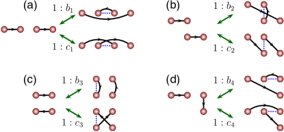
Figure 1: On the left hand side of the reversible arrows, we demonstrate four possible short bond pairs which are connected by a common edge in the lattice; whereas one the right hand side of the arrows, we show two other valence bond tilings of the four sites. Blue dashed lines are the reference edge. The ratios mark the relative amplitudes of the short bonds and the correlated-bond-pairs in the wavefunction coefficients.

We impose the translational and rotational symmetries to the wavefunction to reduce the number of variational parameters. This restriction is perfectly valid as long as we work with finite size systems. There are four distinct arrangements of two short bonds that are connected by a common lattice edge, as illuminated in Fig. 1, therefore eight different correlated-bond-pairs whose amplitudes are denoted by $b_{1},b_{2},b_{3},b_{4}$ and $c_{1},c_{2},c_{3},c_{4}$. Hereafter, we use the word “correlated-bond-pair” and its amplitude interchangeably. Given these clarifications, we can write the trial wavefunction as following

$$|\Psi\rangle=\sum_{C(\alpha)}\prod_{i=1}^{4}b_{i}^{n_{b_{i}}}\prod_{i=1}^{4}c_{i}^{n_{c_{i}}}|\alpha\rangle\equiv\sum_{C(\alpha)}\psi_{C(\alpha)}|\alpha\rangle,$$ (2)

where $C(\alpha)$ is a compact pack of individual short bonds and correlated-bond-pairs on a lattice which produce a valence bond tiling configuration $|\alpha\rangle$, $n_{b_{i}}$ ($n_{c_{i}}$) is the number of $b_{i}$ ($c_{i}$) in a compact pack $C(\alpha)$. Note that different packing $C(\alpha)$ can generate the same valence bond tiling configuration $|\alpha\rangle$.

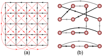
Figure 2: (a) The singlet sign convention for the wavefunction. (b) A transition graph for calculation of the overlap matrix element $\langle{\beta}|{\alpha}\rangle$. The arrows marked for $|\alpha\rangle$ (in black lines) align with the sign convention, whereas for $|\beta\rangle$ (in gray lines) anti-align with the sign convention. $\langle{\beta}|{\alpha}\rangle=(-1)^{n_{v}}2^{n_{l}-\frac{N}{2}}$, where $n_{v}$ is the number of arrows that violate the direction of the flow and $n_{l}$ is the number of loops in the transition graph.

III The variational Monte Carlo method

In this section, we first briefly describe the variational valence bond Monte Carlo method, followed by the optimization method used to determine the optimal variational parameters.

Given a variational wavefunction $|\Psi\rangle$, the expectation value of any operator $\hat{O}$ is written as

$$\frac{\langle\Psi|\hat{O}|\Psi\rangle}{\langle\Psi|\Psi\rangle}=\frac{\sum_{C(\alpha)C(\beta)}W_{C(\alpha)C(\beta)}O_{\alpha\beta}}{\sum_{C(\alpha)C(\beta)}W_{C(\alpha)C(\beta)}},$$ (3)

with the importance sampling weight defined as

$$W_{C(\alpha)C(\beta)}=\psi_{C(\beta)}\psi_{C(\alpha)}\langle\beta|\alpha\rangle,$$ (4)

and the operator matrix element defined as

$$O_{\alpha\beta}=\frac{\langle\beta|\hat{O}|\alpha\rangle}{\langle\beta|\alpha\rangle},$$ (5)

here $\langle\beta|\alpha\rangle$ is the overlap matrix element. If both the coefficients $\psi_{C(\alpha)}$ and the overlap matrix elements $\langle\beta|\alpha\rangle$ are positive definite, we could use the standard valence bond MC method jie1 . However our valence bond configuration $|\alpha\rangle$ allows valence bonds of the same sublattice pairing, therefore the overlap matrix elements can be negative; in addition, the correlated-bond-pair amplitudes can take negative values, which means the coefficients $\psi_{C(\alpha)}$ can be negative too. Thus our wavefunction encounters a negative sign problem. We can treat it in a standard way by rewriting Eq. (3) as

$$\frac{\langle\Psi|\hat{O}|\Psi\rangle}{\langle\Psi|\Psi\rangle} = \frac{\frac{\sum_{C(\alpha)C(\beta)}|W_{C(\alpha)C(\beta)}|\text{Sgn}({W})O_{\alpha\beta}}{\sum_{C(\alpha)C(\beta)}|W_{C(\alpha)C(\beta)}|}}{\frac{\sum_{C(\alpha)C(\beta)}|W_{C(\alpha)C(\beta)}|\text{Sgn}({W})}{\sum_{C(\alpha)C(\beta)}|W_{C(\alpha)C(\beta)}|}}$$ (6)

$$\equiv \frac{\langle\text{Sgn}(W)O_{\alpha\beta}\rangle_{|W|}}{\langle\text{Sgn}(W)\rangle_{|W|}},$$

where $\text{Sgn}(W)$ denotes the sign of the weight Eq. (4). We sample using the absolute value $|W_{C(\alpha)C(\beta)}|$ (abbreviated as $|W|$) as the importance weight. The operator expectation value can be obtained by taking the ratio of $\langle\text{Sgn}(W)O_{\alpha\beta}\rangle_{|W|}$ and $\langle\text{Sgn}(W)\rangle_{|W|}$.

We now explain how to calculate the overlap matrix element $\langle\beta|\alpha\rangle$ and how to count the sign in $\text{Sgn}(W)$. We fix the sign convention for any valence bond in $|\alpha\rangle$: for the AB sublattice pairing, the direction of the valence bond is always pointing from the A sublattice to the B sublattice; whereas for the same sublattice pairing, we refer to the signs drawn in Fig. 2(a) as the convention. Given $|\alpha\rangle$ and $|\beta\rangle$, the overlap matrix element for a transition graph is $(-1)^{n_{v}}2^{n_{l}-\frac{N}{2}}$, where $n_{l}$ is the number of loops in the transition graph and $n_{v}$ is the number of singlets that violate the direction of flow that is arbitrarily chosen for each loop in the transition graph. An example of the transition graph is shown in Fig. 2(b). Here $2^{-N/2}$ is a normalization constant, since the maximum number of loops in a transition graph is $N/2$. The total number of minus sign factors in the coefficient $\psi_{C(\alpha)}$ depends on the sign convention and the signs of the variational parameters $b_{i},c_{i}$. Putting all signs together we have $\text{Sgn(W)}=\text{Sgn}(\psi_{\alpha})\text{Sgn}(\psi_{\beta})\text{Sgn}(\langle\beta|\alpha\rangle)$.

Next, we explain how to calculate the operator matrix element $O_{\alpha\beta}$. Since the singlet product states $|\alpha\rangle,|\beta\rangle$ appear on both the numerator and the denominator, we can choose any singlet sign convention we want (those sign factors will cancel if otherwise choose a difference sign convention). For any transition graph, we choose one such that every loop has $A^{\prime}B^{\prime}A^{\prime}B^{\prime}\cdots A^{\prime}B^{\prime}$ structure, i.e. we choose the sign to be always pointing from $A^{\prime}$ to $B^{\prime}$. Here we use $A^{\prime},B^{\prime}$ to differentiate the $A,B$ sublattices of the original lattice bipartition, and $A^{\prime}$ and $B^{\prime}$ only have a relative meaning within each loop. Therefore all operator expectation values can be evaluated using the same formulas as in the Ref. anders2 with the replacement of $A$ ($B$) by $A^{\prime}$ ($B^{\prime}$).

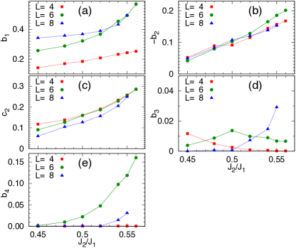
Figure 3: Optimized variational parameters for system sizes $L=4,6,8$ with coupling strength $J_{2}/J_{1}\in[0.45:0.56]$. Parmeters not shown here are optimized close to 0.

The MC sampling of wavefunction Eq. (2) takes two types of update. The first type of update is the local update. We begin by randomly selecting a link from the lattice, one of the following cases will happen:

1. if the link is not occupied by any singlets and it sits beside two individual short bonds, propose to flip randomly to one of the correlated-bond-pairs or stay unchanged with the corresponding probability;

2. if the link belongs to a correlated-bond-pair and is exactly sitting on the reference edge in blue dashed lines in Fig. 1, propose to flip to the two individual short bonds or stay unchanged with the corresponding probability;

3. for any other cases, abandon such a choice and iterate.

If a local update is proposed, we accept or reject this local update with probability $P=\text{min}[2^{n_{l}^{\prime}-n_{l}},1]$, where $n_{l}^{\prime}$ is the number of loop in the trial transition graph. The second type of update is the loop update. We randomly construct an allowed loop of alternating individual short bonds and vacant lattice links, then we shift all individual short bonds on that loop by one lattice space. This rearrangement can always be proposed with probability 1, since all individual short bond have equal amplitudes, and it will keep all the correlated-bond-pairs untouched. The loop update is accepted or rejected with probability $P=\text{min}[2^{n_{l}^{\prime}-n_{l}},1]$ defined above.

We use variational MC to calculate the derivative of the energy with respect to a variational parameter $a$ ($a\in\{b_{i},c_{i}\}$) as

$$\frac{\partial\langle E\rangle}{\partial a}=\langle\frac{n_{a}}{a}E\rangle-\langle\frac{n_{a}}{a}\rangle\langle E\rangle,$$ (7)

and update them according to jie1

$$a({t+1})=a({t})-r\delta({t+1})\times\text{sign}\left(\left(\frac{\partial\langle E\rangle}{\partial a}\right)_{t}\right),$$ (8)

where $t$ is the iteration index, $r$ is a random number $r\in[0,1)$, and $\delta({t})=0.01/t$ until the energy converges. The function form $\delta(t)$ is chosen heuristically jie1 . The optimization results and correlation functions will be presented in the next section.

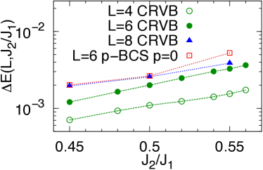
Figure 4: The ground state energy error per site for the $4\times 4$ (green circle), $6\times 6$ (green dots) and $8\times 8$ (blue triangles) lattices, here the reference ground state energies for the $8\times 8$ lattice are taken from the DMRG results in Ref. gong . Red square is a comparison to the projected fermionic BCS wavefunction for a $6\times 6$ lattice without Lanczos projection step huwenjun .

IV The variational Results

We present the well optimized variational parameters for the wavefunction Eq. (2) for system sizes $L=4,6,8$ at $J_{2}/J_{1}\in[0.45:0.56]$ in Fig. 3. We find strong size dependence for the optimized variational parameters $b_{1},b_{3},b_{4}$. However, parameters $b_{2},c_{2}$ have less size dependence. Other parameters that are not shown in Fig. 3 are optimized close to zero. The absolute energy error per site $\Delta E(L,J_{2})$ for sizes $L=4,6$ compared with the exact diagonalization (ED) results richter_ed and for size $L=8$ compared with the DMRG results gong are presented in Fig. 4. The absolute errors are small, e.g., $\Delta E(4,0.55J_{1})\sim 1.5\times 10^{-3}J_{1}$ and $\Delta E(6,0.55J_{1})\sim 3\times 10^{-3}J_{1}$. For comparison, we draw the Gutzwiller-projected BCS wavefunction results without Lanczos projection huwenjun in the same frame: at $L=6,J_{2}=0.55J_{1}$, our absolute energy error is lower by about $40\%$.

We take the optimized parameters from size $L=8$ to calculate the order parameters and the correlation functions for system sizes $L>8$ until the average signs are no longer manageable, because optimizing variational parameters for $L>8$ becomes not feasible. We assume that the correlation functions at larger sizes will not be too sensitive to the variational parameters as long as they are within a reasonable range from the optimal values.

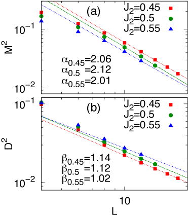
Figure 5: (a) The sublattice magnetization and (b) the dimer order parameter as a function of system size at $J_{2}/J_{1}=0.45,0.5,0.55$ in a log-log plot. Power law functions $M^{2}\sim 1/L^{\alpha}$, $D^{2}\sim 1/L^{\beta}$ have been fitted to the points for $L\geq 10$.

Let us first define a set of order parameters. The sublattice magnetization is written as

$$M^{2}=\frac{1}{N}\sum_{\mathbf{r}}C(\mathbf{r}),$$ (9)

where $\mathbf{r}=(x,y)$, $C(\mathbf{r})$ is the spin correlation function, and it is defined as

$$C(\mathbf{r})=\frac{(-1)^{x+y}}{N}\sum_{i=1}^{N}\mathbf{S}_{\mathbf{r}_{i}}\cdot\mathbf{S}_{\mathbf{r}_{i}+\mathbf{r}}.$$ (10)

The dimer order parameter is defined as

$$D^{2}=D_{x}^{2}+D_{y}^{2},$$ (11)

where

$$D_{x} = \frac{1}{N}\sum_{i}^{N}(-1)^{x_{i}}\mathbf{S}_{\mathbf{r}_{i}}\cdot\mathbf{S}_{\mathbf{r}_{i}+\mathbf{e}_{x}},$$ (12)

$$D_{y} = \frac{1}{N}\sum_{i}^{N}(-1)^{y_{i}}\mathbf{S}_{\mathbf{r}_{i}}\cdot\mathbf{S}_{\mathbf{r}_{i}+\mathbf{e}_{y}},$$ (13)

and $\mathbf{e}_{x}=(1,0)$, $\mathbf{e}_{y}=(0,1)$.

The sublattice magnetization and the dimer order parameter are presented in log-log plots in Fig. 5. The sublattice magnetization at couplings $J_{2}/J_{1}=0.45,0.5,0.55$ scale as $M^{2}\sim 1/L^{2}$, which is expected for the exponentially decaying spin correlation function Eq. (10). The dimer order parameter follows a power law decay with system size as $D^{2}\sim 1/L^{\beta}$ where $\beta\approx 1$. Therefore, we find a critical phase that has gapless singlet excitations and gaped triplet excitations within the range of $J_{2}/J_{1}\in[0.45:0.56]$.

We next make some connections to the results given by previous work. A large optimal parameter $b_{1}$ is consistent with the results of an enhanced spin-spin correlation along the $x$ and $y$ axes shown in Ref. kevin2 . A negative optimal parameter $b_{2}$ is consistent with the result of having negative $h(1,2)$ in the simulation using an AP product state jie1 ; kevin2 . Our variational term $c_{2}$ generates configuration of parallel diagonal bond pair. The parallel diagonal bond pairs together with the short bonds, if contribute with equal weights to the resonating wavefunction on a square lattice, will give a $\mathbb{Z}_{2}$ spin liquid state HongZ2 . Our optimized wavefunction, which contains both the parallel diagonal bonds and the short bonds, does not behave like a $\mathbb{Z}_{2}$ spin liquid, although it deviates from the special point of equal weights superposition defined in Ref. HongZ2 . We need to do further investigation to answer why it fails to be a $\mathbb{Z}_{2}$ spin liquid. The optimal parameter $b_{3}$ at system size $L=8$ grows rapidly as a function of $J_{2}$, whose effect is to increase the dimer-dimer correlation. However given this optimized parameter strength, the effect of $b_{3}$ will not induce a quantum phase transition from a critical phase to the VBS phase as predicted in Ref gong , because the latter phase requires a very large value in $b_{3}$ lin_cap .

Let us turn to the question that we asked earlier: does a negative amplitude $h(2,1)$ in an AP state indicate a phase transition? From our example, the answer seems to be NO. The critical phase presented in our work is simply a result of muting all the long range bonds in the AP state, as one increase the weights of $b_{2}$ and $c_{2}$ from 0, there are no signs of a phase transition from the critical phase to either $\mathbb{Z}_{2}$ or VBS states. Therefore we conclude that the negative amplitude $h(2,1)$ along in an AP state could not trigger a phase transition.

V Conclusion

Using the correlated valence bond state, we minimized the ground state energy of the $J_{1}-J_{2}$ antiferromagnetic (AF) Heisenberg model on a square lattice for a coupling ratio $J_{2}/J_{1}\in[0.45:0.56]$ by turning a few correlated-bond-pair amplitudes. The energies are consistent with the exact diagonalization (ED) results on the $4\times 4$ and $6\times 6$ tori richter_ed and the density matrix renormalization group (DMRG) results on the $8\times 8$ torus gong . We applied the optimal variational parameters from the $8\times 8$ system to the larger tori and studied their correlation functions using the valence bond Monte Carlo (MC) sampling method. We found that within the optimized phase, the Neel order parameter scales as the inverse of the volume, and the dimer order parameter describing the columnar or plaquette valence bond solid (VBS) phases follows a power law decay with the system size $L$ approximately as $1/L$. These correlation functions indicate a critical phase with gapless singlet excitations and gaped triplet excitations in the entire range of $J_{2}/J_{1}\in[0.45:0.56]$. Due to the negative sign problem, we can not optimize even larger systems or further increase the number of variational parameters, such as turn on the individual long range bonds. Our simulation provide insights of how and when the critical phase can turn into a VBS or a $\mathbb{Z}_{2}$ spin liquid. However with the current results, we can not conclude which one is the true ground state with the intermediate coupling strength.

Acknowledgment– We thank J. Richter for providing us the ED results. We would like to thank O. Motrunich, F. Verstraete, K. Beach, A. Sandvik, Z.-C. Gu, S.-S. Gong, W.-J. Hu for useful discussion. The author especially thanks O. Motrunich for reading and giving comments on the manuscript. This work was supported by the Institute for Quantum Information and Matter, an NSF Physics Frontiers Center with support of the Gordon and Betty Moore Foundation through Grant GBMF1250.

References

- (1) P. W. Anderson, Resonating Valence Bonds: A new kind of Insulator?, Mat. Res. Bull. 8, 153 (1973).
- (2) P. W. Anderson, The Resonating Valence Bond State in and Superconductivity, Science 235, 4793 (1987).
- (3) M. Inui, S. Doniach and M. Gabay, Doping dependence of antiferromagnetic correlations in high-temperature superconductors, Phys. Rev. B 38, 6631 (1988).
- (4) K. B. Lyons, P. A. Fleury, L. F. Schneemeyer and J. V. Waszczak, Spin Fluctuations and Superconductivity in , Phys. Rev. Lett. 60, 732 (1988).
- (5) P. A. Lee, N. Nagaosa and X. G. Wen, Doping a Mott insulator: Physics of high-temperature superconductivity, Phys. Mod. Phys. 78, 17 (2006).
- (6) P. Chandra and B. Doucot, Possible spin-liquid state at large S for the frustrated square Heisenberg lattice, Phys. Rev. B 38, 9335 (1988).
- (7) F. Figueirido, A. Karlhede, S. Kivelson, S. Sondhi, M. Rocek and D. S. Rokhsar, Exact diagonalization of finite frustrated spin-1/2 Heisenberg models, Phys. Rev. B 41, 4619 (1990).
- (8) H. J. Schulz, T. A. L. Ziman and D. Poilblanc, Magnetic Order and Disorder in the Frustrated Quantum Heisenberg Antiferromagnet in Two Dimensions, J. Phys. I 6, 675 (1996).
- (9) L. Capriotti, F. Becca, A. Parola and S. Sorella, Resonating Valence Bond Wave Functions for Strongly Frustrated Spin Systems, Phys. Rev. Lett. 87, 097201 (2001).
- (10) J. Richter and J. Schulenburg, The spin-1/2 - Heisenberg antiferromagnet on the square lattice: Exact diagonalization for N=40 spins, Eur. Phys. J. B 73, 117 (2010).
- (11) T. Li, F. Becca, W. Hu and S. Sorella, Gapped spin-liquid phase in the J1-J2 Heisenberg model by a bosonic resonating valence-bond ansatz , Phys. Rev. B 86, 075111 (2012).
- (12) L. Wang, Z.-C. Gu, F. Verstraete and X.-G. Wen, Spin-liquid phase in spin-1/2 square Heisenberg model: A tensor product state approach , (2011), eprint arXiv:1112.3331 (unpublished).
- (13) H.-C. Jiang, H. Yao and L. Balents, Spin liquid ground state of the spin-1/2 square Heisenberg model, Phys. Rev. B 86, 024424 (2012).
- (14) W.-J. Hu, F. Becca, A. Parola and S. Sorella, Direct evidence for a gapless Z2 spin liquid by frustrating Ne ̵́el antiferromagnetism, Phys. Rev. B 88, 060402(R) (2013).
- (15) V. Kalmeyer and R. B. Laughlin, Equivalence of the resonating-valence-bond and fractional quantum Hall states, Phys. Rev. Lett. 59, 2095 (1987).
- (16) X.-G. Wen, F. Wilczek and A. Zee, Chiral Spin States and Superconductivity, Phys. Rev. B 39, 11413(1989).
- (17) X.-G. Wen, Mean Field Theory of Spin Liquid States with Finite Energy Gaps and Topological Order, Phys. Rev. B 44, 2664 (1991).
- (18) N. Read and S. Sachdev, Large-N expansion for frustrated quantum antiferromagnets, Phys. Rev. Lett. 66, 1773 (1991).
- (19) R. Moessner and S. L. Sondhi, Resonating Valence Bond Phase in the Triangular Lattice Quantum Dimer Model, Phys. Rev. Lett. 86, 1881 (2001).
- (20) Hong Yao, and S. A. Kivelson, Exact Spin Liquid Ground States of the Quantum Dimer Model on the Square and Honeycomb Lattices, (2011), eprint arXiv:1112.1702(unpublished).
- (21) J. S. Helton, K. Matan, M. P. Shores, E. A. Nytko, B. M. Bartlett, Y. Yoshida, Y. Takano, A. Suslov, Y. Qiu, J.-H. Chung, D. G. Nocera and Y. S. Lee, Spin Dynamics of the Spin-1/2 Kagome Lattice Antiferromagnet , Phys. Rev. Lett. 98, 107204 (2007).
- (22) S. Yamashita, Y. Nakazawa, M. Oguni, Y. Oshima, H. Nojiri, Y. Shimizu, K. Miyagawa and K. Kanoda, Thermodynamic properties of a spin-1/2 spin-liquid state in a -type organic salt, Nature Physics 4, 459 (2008).
- (23) M. Yamashita, N. Nakata, Y. Senshu, M. Nagata, H. M. Yamamoto, R. Kato, T. Shibauchi and Y. Matasuda, Highly Mobile Gapless Excitations in a Two-Dimensional Candidate Quantum Spin Liquid, Science 328, 1246 (2010).
- (24) Simeng Yan, D. A. Huse, and S. R. White, Spin-Liquid Ground State of the Kagome Heisenberg Antiferromagnet, Science 332, 1173 (2011).
- (25) S. Depenbrock, I. P. McCulloch and U. Schollwock, Nature of the Spin Liquid Ground State of the S=1/2 Kagome Heisenberg Model , Phys. Rev. Lett. 109, 067201 (2012).
- (26) M. P. Gelfand, R. R. P. Singh and D. A. Huse, Zero-temperature ordering in two-dimensional frustrated quantum Heisenberg antiferromagnets, Phys. Rev. B 40, 10801 (1989).
- (27) A. V. Chubukov and Th. Jolicoeur, Dimer stability region in a frustrated quantum Heisenberg antiferromagnet, Phys. Rev. B 44, 12050 (1991).
- (28) P. Chandra, P. Coleman and A. I. Larkin, Ising Transition in Frustrated Heisenberg Models, Phys. Rev. Lett. 64, 88 (1990).
- (29) S. Sachdev and R. N. Bhatt, Bond-operator representation of quantum spins: Mean field theory of frustrated quantum Heisenberg antiferromagnets, Phys. Rev. B 41, 9323 (1990).
- (30) E. Dagotto and A. Moreo, Phase diagram of the frustrated spin-1/2 Heisenberg antiferromagnet in 2 dimensions, Phys. Rev. Lett. 63, 2148 (1989).
- (31) H. J. Schulz and T. A. L. Ziman, Finite-Size Scaling for the Two-Dimensional Frustrated Quantum Heisenberg Antiferromagnet, Europhys. Lett. 18, 355 (1992).
- (32) T. Einarsson and H. J. Schulz, Direct calculation of the spin stiffness in the - Heisenberg antiferromagnet, Phys. Rev. B 51, 6151 (1995).
- (33) L. Capriotti and S. Sorella, Spontaneous Plaquette Dimerization in the - Heisenberg Model, Phys. Rev. Lett. 84, 3173 (2000).
- (34) J. Sirker, Z. Weihong, O. P. Sushkov and J. Oitmaa, - model: First-order phase transition versus deconfinement of spinons, Phys. Rev. B 73, 184420 (2006).
- (35) R. Darradi, O. Derzhko, R. Zinke, J. Schulenburg, S. E. Krüger and J. Richter, Ground state phases of the spin-1/2 - Heisenberg antiferromagnet on the square lattice: A high-order coupled cluster treatment, Phys. Rev. B 78, 214415 (2008).
- (36) K. S. D. Beach, Master equation approach to computing RVB bond amplitudes, Phys. Rev. B 79, 224431 (2009).
- (37) M. Mambrini, A. Läuchli, D. Poilblanc and F. Mila, Plaquette valence-bond crystal in the frustrated Heisenberg quantum antiferromagnet on the square lattice, Phys. Rev. B 74, 144422 (2006).
- (38) M. Arlego and W. Brenig, Plaquette order in the -- model: Series expansion analysis, Phys. Rev. B 78, 224415 (2008).
- (39) V. Murg, F. Verstraete and J. I. Cirac, Exploring frustrated spin systems using projected entangled pair states, Phys. Rev. B 79, 195119 (2009).
- (40) S.-S. Gong, W. Zhu, D. N. Sheng, O. I. Motrunich and M. P. A. Fisher, Plaquette Ordered Phase and Quantum Phase Diagram in the Spin-1/2 Square Heisenberg Model, Phys. Rev. Lett. 113, 027201 (2014).
- (41) A. W. Sandvik, Finite-size scaling and boundary effects in two-dimensional valence-bond solids, Phys. Rev. B 85, 134407 (2012).
- (42) D. Poilblanc, N. Schuch, D. Pèrez-García and J. I. Cirac, Topological and Entanglement Properties of Resonating Valence Bond wavefunctions, Phys. Rev. B 86, 014404 (2012).
- (43) J. Lou and A. W. Sandvik Variational ground states of two-dimensional antiferromagnets in the valence bond basis, Phys. Rev. B 76, 104432 (2007).
- (44) X. Zhang and K. S. D. Beach Resonating valence bond trial wave functions with both static and dynamically determined Marshall sign structure, Phys. Rev. B 87, 094420 (2013).
- (45) A. F. Albuquerque and F. Alet, Critical correlations for short-range valence-bond wavefunctions on the square lattice, Phys. Rev. B 82, 180408R (2010).
- (46) Y. Tang, A. W. Sandvik and C. L. Henley, Properties of resonating valence bond spin liquids and critical dimer models, Phys. Rev. B 84, 174427 (2011).
- (47) Y.-C. Lin, Y. Tang, J. Lou and A. W. Sandvik, Correlated valence-bond states, Phys. Rev. B 86, 144405 (2012).
- (48) L. Wang, D. Poilblanc, Z.-C. Gu, X.-G. Wen and F. Verstraete, Constructing a Gapless Spin-Liquid State for the Spin-1/2 Heisenberg Model on a Square Lattice, Phys. Rev. Lett. 111, 037202 (2013).
- (49) S. Liang, B. Doucot and P. W. Anderson, Some New Variational Resonating-Valence-Bond-Type Wave Functions for the Spin-1/2 Antiferromagnetic Heisenberg Model on a Square Lattice, Phys. Rev. Lett. 61, 365 (1988).
- (50) W. Marshall, Antiferromagnetism, Proc. R. Soc. Lond. Ser. A 232, 48 (1955).