Maximal distance travelled by $N$ vicious walkers till their survival

Abstract

We consider $N$ Brownian particles moving on a line starting from initial positions ${\bf{u}}\equiv\{u_{1},u_{2},\dots u_{N}\}$ such that $0<u_{1}<u_{2}<\cdots<u_{N}$. Their motion gets stopped at time $t_{s}$ when either two of them collide or when the particle closest to the origin hits the origin for the first time. For $N=2$, we study the probability distribution function $p_{1}(m|{\bf{u}})$ and $p_{2}(m|{\bf{u}})$ of the maximal distance travelled by the $1^{\text{st}}$ and $2^{\text{nd}}$ walker till $t_{s}$. For general $N$ particles with identical diffusion constants $D$, we show that the probability distribution $p_{N}(m|{\bf u})$ of the global maximum $m_{N}$, has a power law tail $p_{i}(m|{\bf{u}})\sim{N^{2}B_{N}\mathcal{F}_{N}({\bf u})}/{m^{\nu_{N}}}$ with exponent $\nu_{N}=N^{2}+1$. We obtain explicit expressions of the function $\mathcal{F}_{N}({\bf u})$ and of the $N$ dependent amplitude $B_{N}$ which we also analyze for large $N$ using techniques from random matrix theory. We verify our analytical results through direct numerical simulations.

1 Introduction

Extreme value statistics (EVS) is by now a major issue with a variety of applications in several areas of sciences including physics, statistics or finance, to name just a few Gumbel . For $N$ independent and identically distributed (i.i.d.) random variables $y_{1},\cdots,y_{N}$, the distribution of the maximum $y_{\rm max}=\max_{1\leq i\leq N}\,y_{i}$ (or the minimum $y_{\rm min}$) is well understood with the identification, in the large $N$ (thermodynamical) limit, of three distinct universality classes, depending on the parent distribution of the $y_{i}$’s Gumbel . However, these results for i.i.d. random variables do not apply when the random variables are correlated Dean ; KrapivskySatya2003 . Recently, there has been a surge of interest in EVS of strongly correlated random variables, which is very often the interesting case in statistical physics. Physically relevant examples include for instance the extreme statistics of a stochastic process $u(t)$, with strong temporal correlations, like Brownian motion or its variants. Many studies in this context are focused on extremal properties, like the maximum of $u(t)$, over a fixed time interval, $t\in[0,T]$ Revuz99 ; Yor01 ; Borodin02 ; Majumdar04 ; Majumdar05 ; satyacurrsci ; Schehr10 .

However in many cases the length of this time interval is itself a random variable $t_{s}$, which can thus vary from one realization of the stochastic process to another. This time $t_{s}$ is usually strongly correlated to the process $u(t)$ itself. An interesting situation is the case where $t_{s}$ is a “stopping time” Feller , i.e. when it is associated to the stopping of the process $u(t)$ if a certain event occurs for the first time. For example, in a queuing process starting from an initial queue length $l_{0}>0$, $t_{s}$ is the time when the queue length $l_{t}$ becomes zero for the first time (also called the “busy period”) Kearney04 ; Kearney06 . In finance $t_{s}$ might correspond to the time when a stock price $S_{t}$ reaches some specified level for the first time Yor01 ; Comtet98 ; majum-Qfin . Stopping times also naturally arise in various statistical physics models ranging from capture processes Bramson91 ; Wenbo01 or target annihilating problems Blumen84 all the way to reaction-diffusion kinetics Kang85 ; Ben-Naim93 ; Krapivsky95 or coarsening dynamics of domain walls in Ising model Bray94 . In the context of stochastic control theory, stochastic processes with “stopping time” have been widely studied Shiryaev .

The simplest example of a “stopped” stochastic process is the motion of a single Brownian particle starting form $u(0)=u_{1}>0$ which is observed till time $t_{s}$ when the walker crosses the origin for the first time. This time is called the first passage time Rednerbook ; Bray13 . A natural extreme value question is then: what is the distribution $p(m|u_{1})$ of the maximal displacement $m=\max_{0\leq t\leq t_{s}}u(t)$ travelled by the walker till its first passage time $t_{s}$ ? It can be shown Kearney05 that the cumulative probability $Q_{1}(u_{1}|L)=\text{Prob}[m\leq L|u_{1}]$ that the maximum stays below $L$ till the first passage time is given by $Q_{1}(u_{1}|L)=1-{u_{1}}/{L}$, hence $p(m|u_{1})={u_{1}}/{m^{2}}$. In the context of polymer translocation through a small pore, the quantity $1-Q_{1}(u_{1}|L)$ is precisely the probability of complete translocation of a polymer of length $L$. For generic subdiffusive process, this translocation probability is shown to scale as $\sim(u_{1}/L)^{\phi}$ for large $L$ with $\phi=\theta_{p}/H$ where $\theta_{p}$ is the persistence exponent Bray13 ; Satyacurrsci99 and $H$ is the Hurst exponent Satyarosso10 . Other related questions like the statistics of the time when the walker reaches the maximal displacement before its first passage time $t_{s}$ or the fluctuations of the area enclosed under the Brownian motion till $t_{s}$, have also been studied in connection with several applications including queuing theory or lattice polygon models Kearney04 ; Kearney06 ; Kearney05 ; Kearney07 ; Randon-Furling07 ; Abundo13 .

“Stopped” processes involving $N>1$ particles are also interesting and have been considered in the literature. For instance, the maximal displacement between the “leader" and the “laggard" among $N$ particles has been studied for $N=3$ particles in Ref. SatyaBray2010 . Very recently the authors of Ref. KrapivskySatya2010 have studied the probability distribution function (PDF) $p(m|{\bf{u}})$ of the global maximum $m_{N}$ of $N$ non-interacting and identical Brownian walkers (i.e. with the same diffusion constant) before their first exit from the positive half-line, given that they had started from positions ${\bf{u}}\equiv\{u_{1},u_{2},\dots u_{N}\}$. They showed that the tail of the PDF $p(m|{\bf{u}})$ of the global maximum $m_{N}$ till the time $t_{s}$ when any one of the $N$ walkers crosses the origin for the first time, is given by

$$p(m|{\bf{u}})\simeq\left[N~{}b_{N}\prod_{i=1}^{N}u_{i}\right]~{}\frac{1}{m^{N+1}}\;,\;m\gg u_{N}\;,$$ (1)

where $b_{N}$ is an $N$-dependent constant that behaves for large $N$ as, $b_{N}\approx\text{exp}\left[\frac{N}{2}\log(\log N)\right]$. This result (1) holds for non-interacting particles and it is natural to wonder about the effects of interactions on the statistics of the global maximum till the stopping time of this multi-particle process.

This is precisely the question which we address in this article, by considering non-intersecting Brownian motions, which is one of the simplest – though non trivial – interacting particles system. More precisely, we consider $N$ Brownian walkers moving on a line with position $u_{i}(t)$ at time $t$ for $i=1,2,\dots,N$. They evolve with time according to the Langevin equations

$$\frac{d}{dt}u_{i}(t)=\eta_{i}(t),~{}~{}\text{with}~{}~{}\langle\eta_{i}(t)\rangle=0~{}~{}\text{and}~{}~{}\langle\eta_{i}(t)\eta_{j}(t^{\prime})\rangle=2D_{i}\delta_{ij}\delta(t-t^{\prime})\;,$$ (2)

where $D_{i}$ is the diffusion constant of the $i\text{th}$ particle and $\eta_{i}$’s are independent Gaussian white noises. The initial positions of these particles are $u_{i}(0)=u_{i}$ such that $0<u_{1}<u_{2}<\dots<u_{N}$. The process gets stopped at a random time $t=t_{s}$ when a specific event occurs. In this paper we consider two different mechanisms of stopping event called “process 1” [see Fig. 1 (i)] and “process 2” [see Fig. 1 (ii)]:

• In “process 1”, we consider the evolution of the $N$ Brownian walkers till time $t_{s}$ when either the first particle crosses the origin for the first time before any two walkers meet each other or any two particles meet for the first time before the first particle crosses the origin [see Fig. 1 (i)].

• In “process 2”, $t_{s}$ is the time when the first particle crosses the origin for the first time before any two walkers meet [see Fig. 1 (ii)].

In both cases, the trajectories of the particles are non-intersecting. In the physics literature, such non-intersecting Brownian motions are called “vicious walkers” deGennes68 ; Fisher84 and have been recently studied in various contexts Schehr08 ; Kobayashi ; Nadal09 ; Forrester08 ; Izumi11 ; Rambeau11 ; Issac .

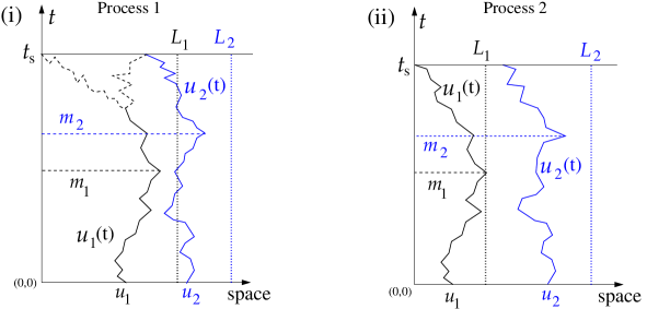
Figure 1: (Color online) Schematic representation of the process 1 and process 2 with $N=2$ particles: $u_{1}(t)$ represents the trajectory of the 1st particle (the leftmost one) and $u_{2}(t)$ represents the trajectory of the 2nd particle (the rightmost one).

Let $p_{i}(m|{\bf{u}})dm$, with $i=1,2,\cdots,N$, denote the probability that $m_{i}\in[m,m+dm]$, where $m_{i}=\max_{0\leq t\leq t_{s}}u_{i}(t)$ is the maximal distance travelled by the $i$th walker till the stopping time $t_{s}$. Here we mainly focus on the PDFs $p_{1}(m|{\bf{u}})$ and $p_{N}(m|{\bf{u}})$ because $m_{1}$ and $m_{N}$ provide characterization of certain geometrical properties of the Brownian walker trajectories. For instance, one may think about $m_{1}$ as an estimate of the common region visited by all the $N$ walkers till the process “stops” (given that all the particles initially started very close to the origin). Similarly, $m_{N}$ characterizes the number of distinct sites visited by the $N$ walkers till $t_{s}$. Recently we have studied the distributions of the number of distinct sites and common sites visited by $N$ independent walkers over a fixed time interval $[0,t]$ Anupam13 . Our initial motivation was to generalize this case to interacting walkers over a fixed time interval. But it is a harder problem to solve. However we show in this paper that the problem with a “stopping time” is solvable even in the presence of interactions. It is also interesting to note that introducing an extra random variable namely the “stopping time” $t_{s}$ renders the problem analytically tractable.

Before presenting the details of our calculations, it is useful to give a summary of our results. We first study the $N=2$ particle problem because it is fully solvable even when the diffusion constants of the two particles are different i.e $D_{1}\neq D_{2}$ and also because the basic concepts are easy to present in this case. Solving a backward Fokker-Planck (BFP) equation we are able to find the full distributions $p_{2}(m|u_{1},u_{2})$ and $p_{1}(m|u_{1},u_{2})$ corresponding to the maximal displacements $m_{2}$ and $m_{1}$ of the right and left particle, respectively (see Fig. 1). We show explicitly for both processes 1 and 2 that the PDFs $p_{2}(m|u_{1},u_{2})$ and $p_{1}(m|u_{1},u_{2})$ have power law tails valid for $m\gg u_{2}$, as

$$p_{1}(m|u_{1},u_{2}) \simeq \dfrac{\mathcal{A}_{1}(u_{1},u_{2},D_{1},D_{2})}{m^{\nu_{1}}}\;,$$ (3)

$$p_{2}(m|u_{1},u_{2}) \simeq \dfrac{\mathcal{A}_{2}(u_{1},u_{2},D_{1},D_{2})}{m^{\nu_{2}}},$$ (4)

$$\text{with~{}exponents}~{}~{}~{}~{}~{}~{}~{}~{}\nu_{1}=\nu_{2} = \frac{3\pi-2\arctan\left(\sqrt{\frac{D_{1}}{D_{2}}}\right)}{\pi-2\arctan\left(\sqrt{\frac{D_{1}}{D_{2}}}\right)}\;.$$ (5)

The functions $\mathcal{A}_{i}(u_{1},u_{2},D_{1},D_{2})$ are the amplitudes associated to the algebraic tails of the PDF $p_{i}(m|u_{1},u_{2})$ with $i=1,2$. While these amplitudes differ from process 1 to process 2, the exponents $\nu_{1}=\nu_{2}$ (for the right and left walkers) are process independent. The amplitudes depend explicitly on the initial positions $u_{1},~{}u_{2}$ as well as on the diffusion constants $D_{1},~{}D_{2}$. Explicit expressions of $\mathcal{A}_{i}(u_{1},u_{2},D_{1},D_{2})$ for both processes 1 and 2 are given in Eqs. (113) to (116).

Next we consider the general $N$-particle problem. In this case, based on the results for the non-interacting case [Eq. (1)] as well as on the results of the $N=2$-particle problem, one generally expects that the PDF $p_{i}(m|{\bf{u}})$ of the maximal distance $m_{i}$ of the $i^{\text{th}}$ particle till the stopping time $t_{s}$, has an algebraic tail:

$$p_{i}(m|{\bf{u}})\simeq\mathcal{A}_{i}({\bf{u},D})~{}\frac{1}{m^{\nu_{i}}},\;\;m\gg u_{N},\;\;i=1,2,\cdots N\;.$$ (6)

The exponents $\nu_{i}$’s and the amplitudes $\mathcal{A}_{i}$’s are, in general, different for the two processes for $N>2$ (note that for $N=2$, while the exponents are same, the amplitudes are different). They also depend explicitly on the number of particles $N$ and on the diffusion constants ${\bf{D}}=(D_{1},D_{2},\cdots,D_{N})$. Proving the result in Eq. (6) for any $i=1,2,...,N$ and general $N$ is a hard task. However, one can make some progress for $i=N$ i.e for the maximal distance $m_{N}$ travelled by the rightmost walker. When the walkers are identical i.e. when they have identical diffusion constants $D_{1}=D_{2}=...=D_{N}=D$, we estimate the tail of the PDF $p_{N}(m|{\bf{u}})$ using a heuristic scaling argument based on the distribution $f_{N}(t_{s}|{\bf u})$ of the “stopping time” $t_{s}$. This argument, for both processes 1 and 2, yields :

$$\nu_{N}=N^{2}+1,~{}~{}\text{when}~{}~{}D_{1}=D_{2}=...=D_{N}=D.$$ (7)

We also obtain an explicit expression of the prefactor $\mathcal{A}_{N}({\bf u},D_{1}=D,\cdots,D_{N}=D)$ in Eq. (6). We observe that for identical diffusion constants this prefactor does not depend on $D$ explicitly. Hence suppressing $D$ from the argument, we denote $\mathcal{A}_{N}({\bf u},D_{1}=D,\cdots,D_{N}=D)=\mathcal{A}_{N}({\bf u})$ and show that it is given by

$$\mathcal{A}_{N}({\bf u})\approx N^{2}B_{N}\mathcal{F}({\bf u})\;,~{}~{}\text{with}\;~{}\mathcal{F}({\bf u})=\frac{\mathcal{Y}_{N}({\bf u})}{S_{N}({\bf u})},$$ (8)

$$\text{where}\,~{}\mathcal{Y}_{N}({\bf u})=\prod_{i=1}^{N}u_{i}\;\prod_{1\leq i<j\leq N}(u_{j}^{2}-u_{i}^{2}),$$ (9)

and $S_{N}({\bf u})$ is an exit probability whose value is $1$ for process 1 and smaller than $1$ for process 2 [given in Eq. (86)]. We also present a formal exact expression of the $N$ dependent constant $B_{N}$, which for large $N$, is shown to grow asymptotically as

$$B_{N}\approx\text{exp}\left[\frac{N^{2}}{2}\log N+o(\log N)\right]\;,$$ (10)

where $o(\log N)$ represents terms smaller than $\log N$. This large $N$ asymptotic form of $B_{N}$ should be compared with the corresponding behavior $b_{N}\approx\text{exp}\left[\frac{N}{2}\log(\log N)\right]$ in the non-interacting case in Eq. (1).

The paper is organized as follows. In section 2 we consider the two walkers problem where we evaluate the PDFs $p_{1}(m|u_{1},u_{2})$ and $p_{2}(m|u_{1},u_{2})$ corresponding to $m_{1}$ and $m_{2}$ respectively. In this section we solve a BFP equation, which under the “stopping time” framework becomes a Laplace’s equation. From the solution of the BFP equation we find the distributions of the individual maximal distances of the first and second particles. In section 3 we consider the general $N$-particle problem. This section is divided into two subsections. In the first subsection 3.1, we give a heuristic scaling argument based on the distribution of the “stopping time” $t_{s}$, to find the exponent $\nu_{N}$ of the power law tail of the PDF $p_{N}(m|{\bf u})$ corresponding to the global maximum $m_{N}$. In the next subsection 3.2, we present a more rigorous calculation based on $N$-particle Green’s function to establish the power law obtained in the previous section 3.1. This calculation also provides exact expressions for the amplitudes associated to the tail of $p_{N}(m|{\bf u})$. Some technical details have been left in Appendices A, B, C and D.

2 Two walkers problem ($N=2$): exact solution

Let us consider the motion of two non-identical Brownian walkers $u_{1}(t)$ and $u_{2}(t)$ given by

$$\dot{u}_{i}(t) = \eta_{i}(t)\;,\text{with}~{}\langle\eta_{i}(t)\rangle=0,~{}\text{for}~{}i=1,2\;,$$ (11)

and $$\langle\eta_{1}(t)\eta_{1}(t^{\prime})\rangle=2D_{1}\delta(t-t^{\prime}),$$ (12)

$$\langle\eta_{2}(t)\eta_{2}(t^{\prime})\rangle=2D_{2}\delta(t-t^{\prime}),$$

$$\langle\eta_{1}(t)\eta_{2}(t^{\prime})\rangle=0,$$

where $D_{1}$ and $D_{2}$ are the diffusion constants of the first (left) and second (right) particle respectively. To compute the PDFs of the individual maximum displacements $m_{1}$ and $m_{2}$, respectively, of the first and second particle, we start by defining the joint cumulative distribution function

$$\mathcal{Q}({\bf{L}}|{\bf{u}})\equiv\mathcal{Q}(L_{1},L_{2}|u_{1},u_{2})=\text{Prob.}[m_{1}\leq L_{1},~{}m_{2}\leq L_{2}|~{}0<u_{1}<L_{1};~{}u_{1}<u_{2}<L_{2}],$$ (13)

given that the initial positional order is maintained till $t_{s}$ and ${\bf{L}}=(L_{1},L_{2})$. The marginal cumulative distribution $\mathcal{Q}_{1}(L|u_{1},u_{2})=\text{Prob.}[m_{1}\leq L|~{}0<u_{1}<L;~{}u_{1}<u_{2}<\infty]$ is obtained by taking the limits $L_{1}\to L$ and $L_{2}\to\infty$ in $\mathcal{Q}({\bf{L}}|{\bf{u}})$ whereas the marginal cumulative distribution $\mathcal{Q}_{2}(L|u_{1},u_{2})=\text{Prob.}[m_{2}\leq L|~{}0<u_{1}<L;~{}u_{1}<u_{2}<L]$ is obtained by taking the limit $L_{1}\to L_{2}=L$ of $\mathcal{Q}({\bf{L}}|{\bf{u}})$.

To find $\mathcal{Q}({\bf{L}}|{\bf{u}})$ we consider a different problem. We consider the first exit problem of a single Brownian walker ${\bf u}(t)=(u_{1}(t),u_{2}(t))$ moving in two dimensions inside the region $\mathcal{W}=$ $OBCD$ described in Fig. 2 (i). We are interested in the probability with which the 2d-walker exits from $\mathcal{W}=$ $OBCD$ through specific boundaries for the first time. We denote this first exit probability by $F({\bf{u}};{\bf{L}})$ for both processes 1 and 2.

For process 1, the exit probability $F({\bf{u}};{\bf{L}})$ represents the probability that the 2d-walker, starting from position $(u_{1},u_{2})$, exits from the region $\mathcal{W}$ through boundary $OD$ or $OB$ for the first time. When the 2d-walker exits through $OB$, it corresponds, in the original two-particle picture (Fig. 1), to the first (left) particle meeting the second (right) particle before it hits the origin for the first time at $t=t_{s}$ while keeping $m_{1}\leq L_{1}$ and $m_{2}\leq L_{2}$ over $[0,t_{s}]$. In contrast, first exit of the 2d-walker through $OD$ corresponds to the first particle hitting the origin before meeting the second particle for the first time at $t=t_{s}$ while maintaining $m_{1}\leq L_{1}$ and $m_{2}\leq L_{2}$ over $[0,t_{s}]$. On the other hand, for process 2 the function $F({\bf{u}};{\bf{L}})$ represents the probability that the 2d-walker exits from the region $\mathcal{W}$ only through boundary $OD$ for the first time. This exit event, in the two-particle picture, corresponds to the first particle hitting the origin for the first time before the two particles meet each other while keeping $m_{1}\leq L_{1}$ and $m_{2}\leq L_{2}$. In the limit $L_{1}\to\infty$ and $L_{2}\to\infty$, we get the ultimate exit probability

$$S_{2}(u_{1},u_{2})=\lim\limits_{L_{1}\to\infty}\lim\limits_{L_{2}\to\infty}F({\bf{u}};{\bf{L}}),$$ (14)

which, for process 1, represents the the probability that the first particle hits either the origin or the second particle ultimately. Of course this occurs with probability $S_{2}(u_{1},u_{2})=1$ in this case. On the other hand, for process 2, $S_{2}(u_{1},u_{2})$ represents the probability that the first particle hits the origin for the first time before it collides with the second particle. This exit probability $S_{2}(u_{1},u_{2})$, in case of process 2, is precisely the survival probability of a lamb in the so-called “lamb-lion” problem where it is being chased by a single diffusing lion in the presence of a refuge. If we identify the first particle as the lamb, the second particle as the lion and the origin as the refuge Rednerbook ; Gabel12 then $S_{2}(u_{1},u_{2})$ is the probability that the lamb survives (i.e. reaches the refuge) before being caught by the lion. This probability is smaller than one since there is a finite probability that the lion catches the lamb (i.e. the second particle hits the first particle before the later hits the origin). In particular for process 2, one can show that Gabel12

$$S_{2}(u_{1},u_{2})=1-\arctan\left(\dfrac{u_{1}}{u_{2}}\sqrt{\dfrac{D_{2}}{D_{1}}}\right)\left[\arctan\left(\sqrt{\dfrac{D_{2}}{D_{1}}}\right)\right]^{-1},$$ (15)

which for $D_{1}=D_{2}=D$ becomes independent of $D$ and is given by $S_{2}(u_{1},u_{2})=1-\frac{4}{\pi}\arctan(u_{1}/u_{2})$.

The quantity $S_{2}(u_{1},u_{2})$ has nice interpretations in terms of the trajectories of the two walkers. It represents the volume of a set of trajectories which contains all pairs of such trajectories which, starting from positions $(u_{1},u_{2})$, stay non-intersecting till $t_{s}$, whereas the quantity $F({\bf{u}};{\bf{L}})$ represents the volume of a subset, which contains such pairs of non-intersecting trajectories that are constrained by $m_{1}\leq L_{1}$ and $m_{2}\leq L_{2}$. Hence the ratio $\frac{F({\bf{u}};{\bf{L}})}{S_{2}(u_{1},u_{2})}$ gives the fraction of such pairs of vicious trajectories which have $m_{1}\leq L_{1}$ and $m_{2}\leq L_{2}$. This fraction precisely represents the cumulative probability $\mathcal{Q}({\bf{L}}|{\bf{u}})$ defined in Eq. (13). Hence, if we know the exit probability $F({\bf{u}};{\bf{L}})$, the cumulative probability $\mathcal{Q}({\bf{L}}|{\bf{u}})$ is obtained from

$$\mathcal{Q}({\bf{L}}|{\bf{u}})=\frac{F({\bf{u}};{\bf{L}})}{S_{2}(u_{1},u_{2})},\;\;\;\text{where}~{}~{}S_{2}(u_{1},u_{2})=\lim\limits_{L_{1}\to\infty}\lim\limits_{L_{2}\to\infty}F({\bf{u}};{\bf{L}}).$$ (16)

The next question is then how to compute this exit probability $F({\bf{u}};{\bf{L}})$ in Eq. (16). In the next subsection we show that the probability $F({\bf{u}};{\bf{L}})$ satisfies a Laplace’s equation which we solve with boundary conditions specified for both process 1 and process 2.

2.1 Backward Fokker-Planck equation for $F({\bf{u}};{\bf{L}})$

A powerful tool to study the PDF of first passage times, like $t_{s}$ in our problem [see Fig. (1)], is the backward Fokker-Planck equation Rednerbook ; Bray13 . Here we are actually dealing with functionals of $t_{s}$, $m_{i}=\max\{x_{i}(t),0\leq t\leq t_{s}\}$. For such functional also, it is possible to use an approach based on BFP equation (see Ref. satyacurrsci for a review). Here we write down a BFP equation for the quantity $F({\bf{u}};{\bf{L}})$ treating the initial coordinates $u_{i}$ as independent variables. To do this, we consider trajectories $u_{1}(t)$ and $u_{2}(t)$ of the two Brownian particles over the interval $[0,t_{s}]$, which evolve according to the Langevin Eqs. (2). We first split the time interval $[0,t_{s}]$ into two parts: $[0,\Delta t]$ and $[\Delta t,t_{s}]$. In the first infinitesimal time window $[0,\Delta t]$ the two Brownian particles will move from their initial positions $\{u_{1},u_{2}\}$ to new positions $\{u_{1}+\Delta u_{1},u_{2}+\Delta u_{2}\}$, where

$$\Delta u_{1}=\int_{0}^{\Delta t}\eta_{1}(t^{\prime})dt^{\prime}~{}\text{and}~{}\Delta u_{2}=\int_{0}^{\Delta t}\eta_{2}(t^{\prime})dt^{\prime}\;.$$ (17)

These two new positions are considered as “new" initial positions of the two Brownian particles, respectively, for the evolution in the subsequent time interval $[\Delta t,t_{s}]$. Since the evolution of the positions of the particles are Markovian, we have

$$F({\bf{u}};{\bf{L}})=\Big{\langle}F({\bf{u}}+\Delta{\bf{u}};{{\bf L}})\Big{\rangle}_{\Delta{{\bf u}}}.$$ (18)

By Taylor expanding the right hand side of the above equation in $\Delta u_{1},\Delta u_{2}$ we have

$$F({\bf{u}};{\bf{L}})=F({\bf{u}};{\bf{L}})+\sum_{i=1}^{2}\left[\frac{\partial F}{\partial u_{i}}\left\langle\Delta u_{i}\right\rangle+\frac{1}{2}\frac{\partial^{2}F}{\partial u_{i}^{2}}\left\langle\Delta u_{i}^{2}\right\rangle\right]+\frac{\partial^{2}F}{\partial u_{1}\partial u_{2}}\left\langle\Delta u_{1}\Delta u_{2}\right\rangle+\dots$$ (19)

From the Langevin Eqs. (2) one can easily show that

$$\left\langle\Delta u_{i}\right\rangle=0\;,\;\left\langle\Delta u_{i}\Delta u_{j}\right\rangle=2\delta_{ij}D_{i}\Delta t~{}~{}\text{for}~{}~{}~{}i=1,2\;.$$ (20)

Using these relations in Eq. (19) and keeping only terms of $\mathcal{O}(\Delta t)$ we obtain the following partial differential equation

$$D_{1}\frac{\partial^{2}F}{\partial u_{1}^{2}}+D_{2}\frac{\partial^{2}F}{\partial u_{2}^{2}}=0\;,$$ (21)

with boundary conditions (BCs) determined by the stopping rules, which are thus different for process 1 and process 2. The Eq. (21) is valid over the region $\mathcal{W}=\{0\leq u_{1}\leq L_{1};u_{1}\leq u_{2}\leq L_{2}\}$.

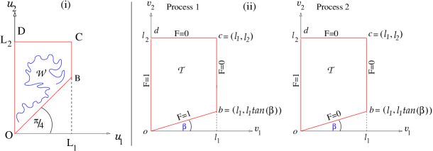
Figure 2: (Color online) (i) Motion of a 2d-walker inside the region $\mathcal{W}$, (ii) Boundaries and boundary conditions associated to the Laplace’s equation in (23) for process 1 and process 2. Note that $l_{i}=L_{i}\sqrt{D_{i}}$ and $\tan(\beta)=\sqrt{D_{1}/D_{2}}$.

It is convenient to perform the following rescaling

$$v_{i}=\frac{u_{i}}{\sqrt{D_{i}}}\;,~{}~{}l_{i}=\frac{L_{i}}{\sqrt{D_{i}}}~{},$$ (22)

which transforms the trapezium OBCD in the $(u_{1},u_{2})$ plane to the trapezium $obcd$ in the $(v_{1},v_{2})$ plane where $\tan(\beta)=\sqrt{D_{1}/D_{2}}$. Under this transformation the Fokker-Planck equation in (21) becomes the Laplace’s equation

$$\frac{\partial^{2}F}{\partial v_{1}^{2}}+\frac{\partial^{2}F}{\partial v_{2}^{2}}=0,$$ (23)

which holds over the region $\mathcal{T}=$ $obcd=\{0\leq v_{1}\leq l_{1};v_{1}\tan(\beta)\leq v_{2}\leq l_{2}\}$ [see Fig. 2 (ii)] with appropriate BCs. We give the BCs in Table 1, which can be understood from the following arguments:

Boundary conditions with $\tan(\beta)=\sqrt{\frac{D_{1}}{D_{2}}}$
Boundary	process 1	process 2
$v_{1}=0$            [od]	$F(v_{1}=0,v_{2};l_{1},l_{2})=1$	$F(v_{1}=0,v_{2};l_{1},l_{2})=1$
$v_{2}=\tan{(\beta)}v_{1}$  [ob]	$F(v_{1},~{}v_{2}=\tan(\beta)v_{1};l_{1},l_{2})=1$	$F(v_{1},~{}v_{2}=\tan(\beta)v_{1};l_{1},l_{2})=0$
$v_{1}=l_{1}$           [bc]	$F(v_{1}=l_{1},v_{2};l_{1},l_{2})=0$	$F(v_{1}=l_{1},v_{2};l_{1},l_{2})=0$
$v_{2}=l_{2}$           [cd]	$F(v_{1},v_{2}=l_{2};l_{1},l_{2})=0$	$F(v_{1},v_{2}=l_{2};l_{1},l_{2})=0$

Table 1: Table of boundary conditions associated to the Laplace’s equation in (23) for process 1 and process 2.

• BC on the segment $[od]$ ($v_{1}=0)$: If the first particle starts with $u_{1}=0$ and $u_{1}\leq u_{2}\leq L_{2}$ (i.e. $v_{1}=0$ and $0\leq v_{2}\leq l_{2}$), then the first particle immediately crosses the origin, which implies $t_{s}=0$, for both process 1 and process 2. Clearly then the maximal displacement of the two particles remains $m_{1}=0<L_{1}$ and $m_{2}=u_{2}\leq L_{2}$ implying the BC $F(v_{1}=0,v_{2};l_{1},l_{2})=1$ on $[od]$ [see Fig. 2 (ii)] for both processes 1 and 2.

• BC on the segment $[ob]$ [$v_{2}=\tan(\beta)v_{1}$]: If both particles start from the same position i.e. $u_{1}=u_{2}<L_{1}<L_{2}$, then they immediately collide implying $t_{s}=0$ and hence, for process 1, $F(v_{1},v_{2}=\tan(\beta)~{}v_{1};l_{1},l_{2})=1$. On the other hand, process 2 excludes the possibility of any collision between the two particles even at time $t=t_{s}$. This implies $F(v_{1},v_{2}=\tan(\beta)~{}v_{1};l_{1},l_{2})=0$ instead of $1$ [see Fig. 2 (ii)].

• BC on the segment $[bc]$ ($v_{1}=l_{1}$): When the initial positions are say $u_{1}=L_{1}$ and $L_{1}\leq u_{2}\leq L_{2}$ (i.e. $v_{1}=l_{1}$ and $l_{1}\leq v_{2}\leq l_{2}$), then clearly $m_{1}=L_{1}$ at $t=0$ and it will definitely become larger than $L_{1}$ in the next subsequent instant. Hence the BC on the segment $[bc]$ is $F(v_{1}=l_{1},v_{2};l_{1},l_{2})=0$ [see Fig. 2 (ii)] for both processes 1 and 2.

• BC on the segment $[cd]$ ($v_{2}=l_{2}$): When the second particle starts from its initial position $u_{2}=L_{2}$ (i.e. $v_{2}=l_{2}$) then $m_{2}=L_{2}$ right at the beginning and $m_{2}$ will definitely become larger than $L_{2}$ in the next subsequent instant implying $F(v_{1},v_{2}=l_{2};l_{1},l_{2})=0$ on the segment $[cd]$ [see Fig. 2 (ii)] for both processes 1 and 2.

To summarize, we finally have to solve a Laplace’s equation in (23), which holds inside the polygon ${\mathcal{T}}$ in the plane $(v_{1},v_{2})$ shown in Fig. 2 with BCs specified in Table 1 for both process 1 and process 2.

2.2 Solution of the Laplace’s equation via conformal mapping

Solving the Laplace’s equation in (23) for any given BC is not a priori an easy task. However using a conformal transformation of the variables, one can transform boundaries of the domain ${\cal T}$ to a much simpler geometry, while leaving the Laplace’s equation itself invariant. Following Ref. SatyaBray2010 , we here use the Schwarz-Christoffel (S-C) transformation which operates as follows: For a polygon $\mathcal{P}$ (see Fig. 3) in the $W$ plane having $n$ vertices $\{w_{1},w_{2},\dots,w_{n}\}$ with corresponding interior angles $\{\alpha_{1},\alpha_{2},\dots,\alpha_{n}\}$, there exists a transformation $W=W(z)$ from complex $z$-plane to $W$ plane such that the upper half $\mathcal{R}^{\prime}$ of the $z$-plane gets mapped onto the interior region $\mathcal{R}$ of the polygon in the $W$ plane. Under this transformation $W=W(z)$, the real axis in the $z$-plane gets mapped onto the boundary of the polygon $\mathcal{P}$ with the $n$ vertices $\{w_{1},w_{2},\dots,w_{n}\}$ being images of the $n$ specific points $\{x_{1},x_{2},\dots,x_{n}\}$ on the real axis. As a result, solving the Laplace’s equation with complicated boundaries reduces to finding the electrostatic potential on the upper half of the complex $z$-plane when the potential is given on the real axis: the electrostatic potential can then be obtained explicitly from the Poisson’s integral formula. The S-C transformation reads as Schaums

$$W(z)=B_{0}~{}\int_{0}^{z}(t-x_{1})^{\frac{\alpha_{1}}{\pi}-1}(t-x_{2})^{\frac{\alpha_{2}}{\pi}-1}\dots(t-x_{n})^{\frac{\alpha_{n}}{\pi}-1}~{}dt+C_{0},$$ (24)

where $B_{0}$ and $C_{0}$ are arbitrary constants. It is convenient to choose one point, say $x_{n}$, at $-\infty$, such that the last factor $(t-x_{n})^{\frac{\alpha_{n}}{\pi}-1}$ present in the integrand of Eq. (24) is absent.

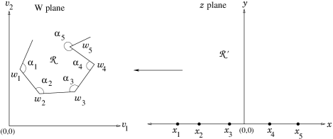
Figure 3: (Color online) Schematic representation of Schwarz-Christoffel transformation $W(z)$ in Eq. (24), such that $w_{i}=W(x_{i})$.

In our problem, we have a trapezium $obcd$ as shown in Fig. 4 for both processes 1 and 2. We chose a point $b^{\prime}$ on the real line of the $z$-plane at $-\infty$, which corresponds to the image of vertex $b$ on the $W$ plane (see Fig. 4). Moreover, let us consider that the points $c^{\prime},d^{\prime},o^{\prime}$ on the real line with coordinates $x=-a,~{}x=-1$ and $x=0$ are mapped onto the vertices $c,d,o$ (see Fig. 4) under the transformation $W(z)$.

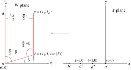
Figure 4: (Color online) Schematic representation of Schwarz-Christoffel transformation in Eq. (25).

One thus has

$$W(z)=B_{0}~{}\int_{0}^{z}t^{-(\frac{\beta}{\pi}+\frac{1}{2})}(t+1)^{-\frac{1}{2}}(t+a)^{-\frac{1}{2}}~{}dt+C_{0},~{}~{}~{}\text{where}~{}~{}~{}\beta=\arctan\left(\sqrt{\frac{D_{1}}{D_{2}}}\right),$$ (25)

where $a$, $B_{0}$ and $C_{0}$ are unknown constants to be determined. Since in our case the origin is mapped onto itself under the transformation $W(z)$, i.e. $W(0)=0$, we have $C_{0}=0$. Hence, from Eq. (25) and Eq. (22) we have

$$\frac{u_{1}}{\sqrt{D_{1}}}+i\frac{u_{2}}{\sqrt{D_{2}}}=W(z)=B_{0}\int_{0}^{z}\frac{dt}{t^{1-\theta}\sqrt{1+t}\sqrt{a+t}}~{}~{}~{}\text{where}~{}~{}~{}\theta=\frac{1}{2}-\frac{1}{\pi}\arctan\left(\sqrt{\frac{D_{1}}{D_{2}}}\right).$$ (26)

Here we note that for $D_{1}=D_{2}$ the exponent $\theta=\frac{1}{4}$. The unknown constants $B_{0}$ and $a$ in Eq. (26) are determined as follows. The points $c^{\prime}\equiv(-a,0)$ and $d^{\prime}\equiv(-1,0)$ on the real axis get mapped onto the points $c\equiv(l_{1}=\frac{L_{1}}{\sqrt{D_{1}}},l_{2}=\frac{L_{2}}{\sqrt{D_{2}}})$ and $d\equiv(0,l_{2})$ on the $W$ plane respectively, which implies

$$d=W(d^{\prime})\implies~{}~{}i~{}l_{1}\alpha\tan(\beta) = B_{0}\int_{0}^{-1}\frac{t^{\theta-1}}{\sqrt{1+t}\sqrt{a+t}}dt,$$ (27)

$$c=W(c^{\prime})\implies~{}~{}l_{1}(1+i~{}\alpha\tan(\beta)) = B_{0}\int_{0}^{-a}\frac{t^{\theta-1}}{\sqrt{1+t}\sqrt{a+t}}dt,$$ (28)

where the variable $\alpha$ is defined as

$$\alpha={L_{2}}/{L_{1}}.$$ (29)

Simplifying Eqs. (27) and (28) one obtains the following two expressions,

$$~{}~{}~{}~{}~{}~{}~{}~{}~{}~{}~{}~{}~{}~{}~{}~{}~{}~{}~{}\frac{h_{\theta}(a)}{k_{\theta}(a)}=\frac{1}{\alpha\tan(\beta)}=\frac{L_{1}\sqrt{D_{1}}}{L_{2}\sqrt{D_{2}}},$$ (30)

$$B_{0}=\frac{l_{1}\alpha\tan(\beta)}{k_{\theta}(a)}~{}e^{i\beta}=\frac{L_{2}}{k_{\theta}(a)\sqrt{D_{2}}}\text{exp}\left[i\arctan\left(\sqrt{\frac{D_{1}}{D_{2}}}\right)\right],$$ (31)

$$\text{with}~{}~{}h_{\theta}(a)=\int_{1}^{a}\frac{t^{\theta-1}}{\sqrt{t-1}\sqrt{a-t}}~{}dt~{}~{}\text{and}~{}~{}~{}k_{\theta}(a)=\int_{0}^{1}\frac{t^{\theta-1}}{\sqrt{1-t}\sqrt{a-t}}~{}dt\;,$$ (32)

which determine the two constants $a$ and $B_{0}$.

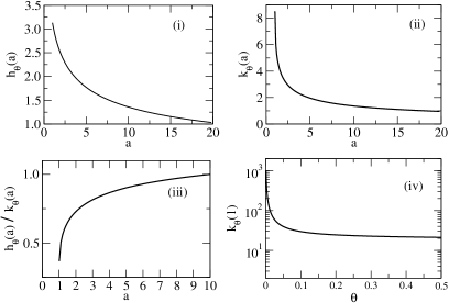
Figure 5: (Color online) Properties of the integrals $h_{\theta}(a)$ and $k_{\theta}(a)$ given in Eq. (32). In figures (i), (ii) and (iii) we have used the value $\theta={1}/{3}$.

The solution of the Eq. (30) gives the value of $a$ for given $\alpha$ and $\beta$ whereas using this solution for $a$ in Eq. (31) we get $B_{0}$. When $\alpha\to 1$, i.e. $L_{1}\to L_{2}$, the vertices $c$ and $b$ of the trapezium $obcd$ approach to each other. This means that the point $c^{\prime}$ on the real axis of the $z$-plane (Fig. 4) should approach $b^{\prime}$ implying $a\to\infty$ as $L_{1}\to L_{2}$. On the other hand, when $\alpha\to\infty$, i.e. $L_{2}\gg L_{1}$, the point $c^{\prime}$ should approach $d^{\prime}$ implying $a\to 1$ in this limit. Hence we expect that the value of $a$ should lie in the interval $[1,+\infty)$ for $1<\alpha<\infty$ where both the integrals $h_{\theta}(a)$ and $k_{\theta}(a)$ are smooth real valued functions of $a$ for given $\theta$. In Fig. 5 (i) and (ii) we show how the integrals $h_{\theta}(a)$ and $k_{\theta}(a)$ behave as a function of $a$ for $\theta=\frac{1}{3}$. Solving the Eq. (30) we obtain the value of $a$ for given $\alpha$ and $\beta$ and using this value of $a$ in Eq. (31) we can get $B_{0}$. In Fig. 6 we plot $a$ as a function of $\alpha$ for $D_{1}=1.3$ and $D_{2}=1.5$ and see that $a$ diverges when $\alpha$ goes to $1$ whereas $a$ approaches $1$ when $\alpha\to\infty$ (as expected from the above arguments). Let us analyze the integrals $h_{\theta}(a)$ and $k_{\theta}(a)$ in detail to see how $a$ behaves as a function of $\alpha$ when $\alpha\to 1$ and $\alpha\to\infty$ separately.

We first consider the case when $\alpha$ approaches $1$ from above i.e. $a\to\infty$. Expanding the two functions entering the left hand side (l.h.s.) of Eq. (30) for large $a$ we get

$$h_{\theta}(a) \simeq \frac{\sqrt{\pi}\Gamma[\theta]}{\sqrt{a}\tan{\beta}}\left[\frac{1}{\Gamma[\frac{1}{2}+\theta]}+\frac{\theta}{\Gamma[\frac{3}{2}+\theta]}\frac{1}{a}+\mathcal{O}(a^{-2})\right],$$ (33)

$$k_{\theta}(a) \simeq \frac{\sqrt{\pi}\Gamma[\theta]}{\sqrt{a}}\left[\frac{1}{\Gamma[\frac{1}{2}+\theta]}+\left(\frac{\theta}{2\Gamma[\frac{1}{2}+\theta]}-\frac{\theta}{4\Gamma[\frac{3}{2}+\theta]}\right)\frac{1}{a}+\mathcal{O}(a^{-2})\right],$$ (34)

where $\Gamma[x]$ is the Gamma function.

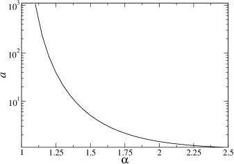
Figure 6: (Color online) Plot of $a$ as a function of $\alpha$ obtained by numerically solving Eq. (30) for a given value of $\beta$ (see Eq. (25)) corresponding to $D_{1}=1.3$ and $D_{2}=1.5$.

Using the above expressions in Eq. (31) we see that $a$ diverges as $a\propto 1/(\alpha-1)$ as $\alpha$ approaches $1$. Next we consider the case $\alpha\to\infty$ where we expect $a$ to approach $1$. Expanding the functions $h_{\theta}(a)$ and $k_{\theta}(a)$ around $a=1$ we find

$$h_{\theta}(a) \simeq \pi+\pi(1-\theta)~{}\tan(\beta)(a-1)+\mathcal{O}\left((a-1)^{2}\right),$$ (35)

$$k_{\theta}(a) \simeq -\log(a-1)+\mathcal{O}\left((a-1)\log(a-1)\right),$$ (36)

which with the help of Eq. (31) yields $a-1\sim e^{-\pi\alpha\tan(\beta)}$. In Table 2 we summarize the values of $a$ and $B_{0}$ for different $\alpha=L_{2}/L_{1}$.

$\alpha\to 1$	$a\propto 1/{(\alpha-1)}$	$B_{0}=\dfrac{L_{1}\Gamma[\frac{1}{2}+\theta]\tan{\beta}}{\sqrt{\pi D_{1}}\Gamma[\theta]}\sqrt{a}e^{i\beta}$
$1<\alpha<\infty$	$1<a<\infty$	$B_{0}=\dfrac{L_{1}\alpha\tan(\beta))}{\sqrt{D_{1}}k_{\theta}(a)}~{}e^{i\beta}$
$\alpha\to\infty$	$a-1\simeq e^{-\pi\alpha\tan(\beta)}$	$B_{0}=\dfrac{L_{1}}{\pi\sqrt{D_{1}}}e^{i\beta}$

Table 2: Table of values of $a$ and $B_{0}$ for given $L_{1}$, $\alpha={L_{2}}/{L_{1}}$ and $\beta=\arctan\left(\sqrt{\frac{D_{1}}{D_{2}}}\right)$.

Once the values of $B_{0}$ and $a$ are determined, the conformal transformation in Eq. (26) is uniquely defined. Under this transformation (26) the Laplace’s equation (23) remains invariant i.e we still have

$$\frac{\partial^{2}F(x,y)}{\partial x^{2}}+\frac{\partial^{2}F(x,y)}{\partial y^{2}}=0\;,$$ (37)

in the new variables $(x,y)$ which holds over the upper half complex plane. The BCs on the real axis are

$$(i)~{}F(x,0)=0~{}\text{for}~{}x<-1~{}~{}\text{and}~{}F(x,0)=1~{}\text{for}~{}x\geq-1~{}~{}~{}~{}~{}\text{(process 1)}$$ (38)

and $$(ii)~{}F(x,0)=1~{}\text{for}~{}-1\leq x\leq 0~{}~{}\text{and}~{}F(x,0)=0~{}\text{otherwise}~{}~{}~{}~{}\text{(process 2)}\;.$$ (39)

The solution of the Laplace’s equation in the upper half complex plane can be written explicitly in terms of the values at the boundary by using Poisson’s integral formula

$$F(x,y)=\frac{y}{\pi}\int_{-\infty}^{\infty}\frac{F(x^{\prime},0)}{y^{2}+(x-x^{\prime})^{2}}dx^{\prime}\;.$$ (40)

Using the BCs in Eqs. (38), (39) and performing the integral in both cases we get the following explicit solutions

$$F(x,y)=\begin{cases}&1-\frac{1}{\pi}\arctan\left(\frac{y}{1+x}\right)~{}~{}~{}~{}~{}~{}~{}~{}~{}~{}~{}~{}~{}~{}~{}~{}~{}~{}~{}~{}~{}~{}\text{for process 1}\\ &\frac{1}{\pi}\left[\arctan\left(\frac{y}{x}\right)-\arctan\left(\frac{y}{1+x}\right)\right]~{}~{}~{}~{}~{}~{}~{}\text{for process 2},\end{cases}$$ (41)

expressed in terms of $x$ and $y$.

2.3 Results and discussions

In the previous section 2.2, we have solved the Laplace’s equation in (23) using S-C conformal mapping which provides the first exit probability $F$ in terms of the $(x,y)$ coordinates (i.e. in the $z$-plane). Then, to obtain the cumulative distribution $\mathcal{Q}(L_{1},L_{2}|u_{1},u_{2})$ defined in Eq. (13), we first need to express the solution $F(x,y)$ in terms of our original coordinates $\left(v_{1}=\frac{u_{1}}{\sqrt{D_{1}}},v_{2}=\frac{u_{2}}{\sqrt{D_{1}}}\right)$ which can, in principle, be done by inverting the conformal transformation $W(z)=W$ in Eq. (26). Once this inversion is performed, the marginal cumulative distribution $\mathcal{Q}_{1}(L|u_{1},u_{2})=\text{Prob.}[m_{1}\leq L|~{}0<u_{1}<L_{1};~{}u_{1}<u_{2}<L_{2}]$ is obtained by taking $L_{1}\to L$ and $L_{2}\to\infty$ limits of $\mathcal{Q}(L_{1},L_{2}|u_{1},u_{2})$ whereas the marginal cumulative distribution $\mathcal{Q}_{2}(L|u_{1},u_{2})=\text{Prob.}[m_{2}\leq L|~{}0<u_{1}<L_{1};~{}u_{1}<u_{2}<L_{2}]$ is obtained by taking $L_{1}\to L_{2}=L$ limit of $\mathcal{Q}(L_{1},L_{2}|u_{1},u_{2})$. The inversion of the transformation $W(z)=W$ for any given $L_{1}$ and $L_{2}$ can not be done analytically in terms of elementary functions but one can do this inversion numerically. In the asymptotic limit $L_{2}\to\infty$ and $L_{1}\to\infty$, as we will show below, the S-C transformation gets simplified and there one can invert the transformation analytically. In section 2.3.1 we evaluate $\mathcal{Q}_{1}(L|u_{1},u_{2})$ and $\mathcal{Q}_{2}(L|u_{1},u_{2})$ obtained by numerical inversion of the conformal transformation. These expressions can then be compared to their numerical estimation obtained by direct simulation of Langevin equations (11). In section 2.3.2 we present large $L$ asymptotics which allows to study the tails of the marginal distributions $p_{i}(m|u_{1},u_{2})$. Finally, in section 2.3.3 we study the correlations between $m_{1}$ and $m_{2}$.

2.3.1 Evaluation of $\mathcal{Q}_{1}(L|u_{1},u_{2})$ and $\mathcal{Q}_{2}(L|u_{1},u_{2})$ through numerical inversion

We first compute $\mathcal{Q}_{1}(L|u_{1},u_{2})$, i.e. the probability that the maximum $m_{1}$ of the 1st particle remains below $L$ till the stopping of the two-particle process. It is obtained from $\mathcal{Q}(L_{1},L_{2}|u_{1},u_{2})$ in the $L_{2}\to\infty$ limit keeping $L_{1}=L$ fixed. This corresponds to $\alpha=L_{2}/L_{1}\to\infty$ which, with the help of table 2, implies $a\to 1$ and $B_{0}=\frac{L}{\pi\sqrt{D_{1}}}e^{i\beta}$ where $\beta$ is given in Eq. (25). Using this value of $B_{0}$ and taking the limit $a\to 1$ of the S-C transformation in Eq. (26) we have

$$\frac{\pi\sqrt{D_{2}u_{1}^{2}+D_{1}u_{2}^{2}}}{L~{}\sqrt{D_{2}}}~{}e^{i\left(\psi-\beta\right)}=\int_{0}^{z}\frac{t^{\theta-1}}{(1+t)}~{}dt,$$ (42)

where we have written the complex coordinate $W=\left(\frac{u_{1}}{\sqrt{D_{1}}}+i\frac{u_{2}}{\sqrt{D_{2}}}\right)$ on the left hand side as

$$W=\frac{\sqrt{D_{2}u_{1}^{2}+D_{1}u_{2}^{2}}}{\sqrt{D_{1}D_{2}}}e^{i\psi},~{}~{}\text{with}~{}~{}\psi=\arctan\left(\frac{\sqrt{D_{1}}u_{2}}{\sqrt{D_{2}}u_{1}}\right).$$ (43)

For given $(u_{1},u_{2})$ and $L$, we numerically solve the above equation (42) for $z=x+iy$. Plugging this solution into Eq. (41) first and then using Eq. (16) we obtain $\mathcal{Q}_{1}(L|u_{1},u_{2})$. In Fig. 7 (i) and (ii) we compare the value of $\mathcal{Q}_{1}(L|u_{1},u_{2})$ obtained from numerical inversion of the transformation $W(z)$ [i.e. solving Eq. (42)] to the value of $\mathcal{Q}_{1}(L|u_{1},u_{2})$ obtained from direct simulation of the Langevin Eqs. (11) for both process 1 and process 2, and for $u_{1}=1.27,~{}u_{2}=3.51$, $D_{1}=1.3$ and $D_{2}=1.5$. We observe a very good agreement between the analytical and numerical curves.

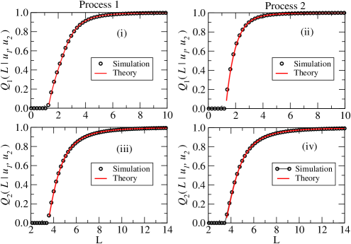
Figure 7: (Color online) Plots of marginal cumulative distributions. The open circles represent the data obtained from numerical simulations while the solid line corresponds to a numerical evaluation of our exact formula. In figures (i) and (ii) we show a plot of $\mathcal{Q}_{1}(L|u_{1},u_{2})$ as a function of $L$ while in figures (iii) and (iv) we show a plot of $\mathcal{Q}_{2}(L|u_{1},u_{2})$ again as a function $L$ for both processes. The parameters used for this plot are $u_{1}=1.27,~{}u_{2}=3.51$,$D_{1}=1.3$ and $D_{2}=1.5$.

Similarly, to evaluate $\mathcal{Q}_{2}(L|u_{1},u_{2})$, i.e. the probability that the maximum $m_{2}$ of the 2nd particle stays below $L$ till $t_{s}$, we first take the limit $L_{2}\to L_{1}=L$ (i.e. $\alpha\to 1$) of $\mathcal{Q}(L_{1},L_{2}|u_{1},u_{2})$. We know from Table 2 that, when $\alpha\to 1$ the coordinate $a$ goes to $\infty$. As a result, the S-C transformation in Eq. (26) now reads

$$\frac{\Gamma[\theta]\Gamma[\frac{1}{2}-\theta]\sqrt{D_{2}u_{1}^{2}+D_{1}u_{2}^{2}}}{L~{}\sqrt{\pi}\sqrt{D_{1}+D_{2}}}~{}e^{i\left(\psi-\beta\right)}=\int_{0}^{z}\frac{t^{\theta-1}}{\sqrt{1+t}}~{}dt\;.$$ (44)

For given $(u_{1},~{}u_{2})$ and $L$, we solve the above equation for $z=x+iy$ numerically and plug the solution into Eq. (41) to obtain $\mathcal{Q}_{2}(L|u_{1},u_{2})$ from Eq. (16). In Fig. 7 (iii) and (iv) we compare the value of $\mathcal{Q}_{2}(L|u_{1},u_{2})$, obtained by numerically inverting the transformation $W(z)$ [i.e. solving Eq. (44)] to the value of $\mathcal{Q}_{2}(L|u_{1},u_{2})$ obtained from direct simulation of the Langevin Eqs. (11) for both process 1 and process 2, and for $u_{1}=1.27,~{}u_{2}=3.51$, $D_{1}=1.3$ and $D_{2}=1.5$: here also one observes a very good agreement between the analytical and numerical curves.

2.3.2 Large $L_{1}$ and $L_{2}$ limits

We now focus on the limit where both $L_{1}$ and $L_{2}$ are large, keeping the ratio $\alpha=L_{2}/L_{1}$ fixed. In this limit, the S-C transformation gets simplified which makes it possible to invert the transformation $W=W(z)$ analytically. For simplicity we present here our calculation assuming $D_{1}=D_{2}=D$. The calculation for $D_{1}\neq D_{2}$ can be done similarly. For $D_{1}=D_{2}=D$ we have

$$\beta=\frac{\pi}{4},~{}~{}\theta=\frac{1}{4},~{}~{}W=\frac{u_{1}+i~{}u_{2}}{\sqrt{D}}=\frac{\sqrt{u_{1}^{2}+u_{2}^{2}}}{\sqrt{D}}e^{i\psi}~{}~{}\text{where}~{}~{}\psi=\arctan\left(\frac{u_{2}}{u_{1}}\right)\;.$$ (45)

From Eq. (31), we see that $B_{0}$ diverges linearly with $L_{1}$ as $k_{\theta}(a)$ is finite (see Fig. 5 ii). Dividing both sides of Eq. (26) by $B_{0}$ and taking $L_{1}\to\infty$ and $L_{2}\to\infty$ limit while keeping $\alpha=L_{2}/L_{1}$ fixed, we see the left hand side of Eq. (26) decreases to zero. This suggests us to expand the integral on the right hand side of Eq. (26) around $z=0$ to get

$$\frac{W}{B_{0}}=\frac{\left(u_{1}+iu_{2}\right)}{B_{0}\sqrt{D}}=\frac{z^{\frac{1}{4}}}{\sqrt{a}}\left[4-\frac{2(1+a)}{5a}z+\mathcal{O}(z^{2})\right].$$ (46)

Following Ref. SatyaBray2010 , we now invert the transformation $W=W(z)$ from $z$-plane to $(u_{1},u_{2})$ plane to obtain $z\approx\mathcal{R}e^{i\Psi}$ where, denoting $L_{1}=L$ and $L_{2}=\alpha L$, we have

$$\mathcal{R} = \left[\mathcal{X}(a)\frac{(u_{1}^{2}+u_{2}^{2})^{2}}{L^{4}}+\frac{2(1+a)\mathcal{X}(a)^{2}}{5a}\frac{(u_{1}^{2}+u_{2}^{2})^{4}\cos\left(4\psi-\pi\right)}{L^{8}}+\mathcal{O}(L^{-12})\right],\allowdisplaybreaks[4]$$ (47)

$$\Psi = 4\psi-\pi+\frac{2(1+a)\mathcal{X}(a)}{5a}\frac{(u_{1}^{2}+u_{2}^{2})^{2}\sin\left(4\psi-\pi\right)}{L^{4}}+\mathcal{O}(L^{-12}),\allowdisplaybreaks[4]$$ (49)

$$\text{with}\;\mathcal{X}(a)=\left(\frac{h_{1/4}(a)\sqrt{a}}{4}\right)^{4},$$

and $h_{1/4}(a)$ is defined in Eq. (32). This large $L$ expansion can in principle be carried out systematically to arbitrary order. We now take the small $z$ limit of the explicit solutions $F(x,y)$ in Eq. (41) and then inject the above large $L$ expansion of $z\approx\mathcal{R}e^{i\Psi}$ into it to get the exit probability, mentioned in Eq. (16), as

$$F(u_{1},u_{2};L,\alpha L)\approx\begin{cases}&1-\dfrac{\mathcal{X}(a)}{\pi}(u_{1}^{2}+u_{2}^{2})^{2}\sin\left(4\psi-\pi\right)L^{-4}+\mathcal{O}(L^{-8})\;\;\;\;\hskip 9.95863pt\text{for process 1}\;,\\ &\\ &\dfrac{4\psi-\pi}{\pi}-\dfrac{1}{\pi}\left(\dfrac{3a-2}{5a}\right)\mathcal{X}(a)(u_{1}^{2}+u_{2}^{2})^{2}\sin\left(4\psi-\pi\right)L^{-4}+\mathcal{O}(L^{-12})\\ &\hskip 227.62204pt\text{for process 2},\end{cases}$$ (50)

where $\psi$ and $\mathcal{X}(a)$ are given in Eq. (45) and (49) respectively, with $a$ implicitly determined from Eq. (30). Putting $L=\infty$ in the above equation (50) we get the probability $S_{2}(u_{1},u_{2})$ defined in Eq. (14), which for process 1 is equal to $1$ and for process 2 is equal to $\frac{4\psi-\pi}{\pi}$. Using the expression of $\psi$ from Eq. (45), we get explicit expression of $S_{2}(u_{1},u_{2})$ for process 2, as announced in Eq. (15) with $D_{1}=D_{2}$. One can follow the same calculation to get $S_{2}(u_{1},u_{2})$ for $D_{1}\neq D_{2}$. After few simplifications, one can rewrite the exit probability $F(u_{1},u_{2};L,\alpha L)$ in Eq. (50) in the following form :

$$F(u_{1},u_{2};L,\alpha L)\approx S_{2}(u_{1},u_{2})-c(a)\mathcal{Y}_{2}(u_{1},u_{2})~{}L^{-4}~{}~{}\text{for}~{}L\gg u_{2},$$ (51)

for both processes 1 and 2, where the constant $c(a)$ is given by

$$c(a)=\begin{cases}&\dfrac{4\mathcal{X}(a)}{\pi},~{}~{}~{}~{}~{}~{}~{}~{}~{}~{}~{}~{}~{}~{}~{}~{}\text{for~{}process 1}\\ &\\ &\dfrac{4\mathcal{X}(a)}{\pi}\left(\dfrac{3a-2}{5a}\right),~{}~{}\text{for~{}process 2},\end{cases}$$ (52)

$$\text{and}~{}~{}\mathcal{Y}_{2}(u_{1},u_{2})=u_{1}u_{2}(u_{2}^{2}-u_{1}^{2})~{}\text{for~{}both~{}processes~{}1~{}and~{}2.}$$ (53)

Plugging the expression of $F(u_{1},u_{2};L,\alpha L)$ from Eq. (51) into Eq. (16), we get the joint cumulative distribution

$$\mathcal{Q}(L,\alpha L|u_{1},u_{2}) \simeq 1-c(a)\frac{\mathcal{Y}_{2}(u_{1},u_{2})}{S_{2}(u_{1},u_{2})}~{}\frac{1}{L^{4}},~{}~{}\text{for}~{}L\gg u_{2}~{}\;.$$ (54)

Note that the $\alpha$ dependence in the above expression comes only through $a$ since it is a function of $\alpha=\frac{L_{2}}{L_{1}}$ [see Eq. (30)]. Taking the limit $\alpha\to\infty$ i.e. $a\to 1$ (see Table 2) in the above expression, we get the marginal cumulative distribution $\mathcal{Q}_{1}(L|u_{1},u_{2})$ [defined below Eq. (13)] of the maximum $m_{1}$ given that the 1st particle always stayed below the 2nd particle till the stopping time $t_{s}$. Similarly, if we take the limit $\alpha\to 1$ i.e. $a\to\infty$ limit, we get $\mathcal{Q}_{2}(L|u_{1},u_{2})$, the cumulative distribution of the maximum $m_{2}$. After taking the derivative of $\mathcal{Q}_{i}(L|u_{1},u_{2})$ with respect to $L$ and putting $L=m$ we get the marginal PDFs, $p_{i}(m|u_{1},u_{2})$ for $i=1,2$ which behave like

$$p_{1}(m|u_{1},u_{2})\approx k_{1}{\mathcal{Y}_{2}(u_{1},u_{2})}\frac{1}{m^{5}},~{}\text{for}~{}m\gg u_{2}\;,$$ (55)

$$p_{2}(m|u_{1},u_{2})\approx k_{2}\frac{\mathcal{Y}_{2}(u_{1},u_{2})}{S_{2}(u_{1},u_{2})}\frac{1}{m^{5}},~{}\text{for}~{}m\gg u_{2}\;,$$ (56)

where the numerical constants $k_{1}$ and $k_{2}$ are obtained by taking, respectively, $a\to 1$ and $a\to\infty$ limits of $c(a)$ and finally multiplying it by $4$ [coming from the derivative of $L^{-4}$ w. r. t. $L$ in (51)]. The constants $k_{1}$ and $k_{2}$ are explicitly given by

$$k_{1}=\begin{cases}&\dfrac{\pi^{3}}{16}\;,\;\text{for~{}process 1}\\ &\\ &\dfrac{\pi^{3}}{80}\;,\;\text{for~{}process 2}\end{cases}\hfill\hskip 28.45274pt{\rm and}\;\hskip 28.45274ptk_{2}=\begin{cases}&\dfrac{\Gamma[\frac{1}{4}]^{8}}{(4\pi)^{3}}\;,~{}~{}~{}~{}\text{for~{}process 1}\\ &\\ &\dfrac{3~{}\Gamma[\frac{1}{4}]^{8}}{5~{}(4\pi)^{3}}\;,~{}~{}\text{for~{}process 2}\;.\end{cases}$$ (57)

We can easily see that the tails of the PDFs $p_{i}(m|u_{1},u_{2})$ in Eq. (56) are of the form announced in Eqs. (3) and (4) with $D_{1}=D_{2}$. The Vandermonde determinant in the expression of $\mathcal{Y}_{2}(u_{1},u_{2})$ (53) reflects the fact that the two walkers are non-intersecting and is reminiscent of the connection between vicious walkers and random matrix theory Schehr08 .

A similar calculation can be performed in the case of different diffusion constants $D_{1}\neq D_{2}$ to obtain

$$\mathcal{Q}(L,\alpha L|u_{1},u_{2})\approx 1-\frac{\mathcal{B}(u_{1},u_{2},\alpha,\mu)}{L^{\mu}}~{}~{}\text{with}~{}~{}\mu=\frac{2\pi}{\pi-2\arctan\left(\sqrt{\frac{D_{1}}{D_{2}}}\right)}~{}~{}~{}\text{for}~{}~{}L\gg u_{2}$$ (58)

which finally provides the PDFs

$$p_{i}(m|u_{1},u_{2})\approx\frac{\mathcal{A}_{i}(u_{1},u_{2},\mu)}{m^{\nu}}~{}~{}\text{with}~{}~{}\nu=\mu+1~{}~{}~{}\text{for}~{}~{}m\gg u_{2}\;.$$ (59)

The explicit expressions of the functions $\mathcal{B}(u_{1},u_{2},\alpha,\mu)$ and $\mathcal{A}_{i}(u_{1},u_{2},\mu)$ have been left in Appendix B. Here we present the results of $p_{1}(m_{1}|u_{1},u_{2})$ and $p_{2}(m_{1}|u_{1},u_{2})$ obtained by simulating directly the Langevin equations in Eq. (2) and compare them with the analytical prediction in Eq. (59).

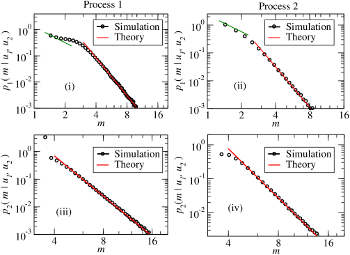
Figure 8: (Color online) Plots of the PDFs of $m_{1}$, the maximum of the first (left) particle and of $m_{2}$, the maximum of the second (right) particle up to the stopping time $t_{s}$. The open circles correspond to numerical simulations while the solid lines represent the exact asymptotic behaviors (the red ones for the large argument asymptotics and the green one for the small argument asymptotics) as explained in the text. There is no fitting parameters. In figures (i) and (ii) we show a plot of $p_{1}(m|u_{1},u_{2})$ as a function of $m$ whereas, in figures (iii) and (iv) we show a plot of $p_{2}(m|u_{1},u_{2})$ as a function of $m$ for both processes. The parameters used for these plots are $u_{1}=1.27,~{}u_{2}=3.51$, $D_{1}=1.3$ and $D_{2}=1.5$. The red solid lines have a slope $-\nu=-4.826$ as expected from Eqs. (58) and (59) while the green solid lines have a slope $-2$.

In Fig. 8 (i) and (ii) we show a plot $p_{1}(m|u_{1},u_{2})$ (with open circles) obtained from simulation, respectively for process 1 and process 2, with $u_{1}=1.27,~{}u_{2}=3.51$, $D_{1}=1.3$ and $D_{2}=1.5$. We have also plotted the large $m$ asymptotic behavior obtained from our analytical prediction (59) with the same set of parameters for which, one expects from Eqs. (58) and (59) that $\nu\simeq 4.826$ and, from Eqs. (113) and (114), $\mathcal{A}_{1}(u_{1},u_{2},\mu)\simeq 68.79$ for process 1 and $\mathcal{A}_{1}(u_{1},u_{2},\mu)\simeq 25.32$ for process 2. We see that the agreement between our numerical simulations and our analytical results is very good. Notice also that for $m_{1}\ll u_{2}$, the first particle does not feel the presence of the second particle and therefore one expects that in this limit $p_{1}(m|u_{1},u_{2})\sim{u_{1}}/{m^{2}}$ for process 1 and $p_{1}(m|u_{1},u_{2})\sim{u_{1}}/{[S_{2}(u_{1},u_{2})m^{2}]}$ for process 2, with $S_{2}(u_{1},u_{2})\simeq 0.549$ in the later case [see Eq. (15)]. These asymptotic behaviors for small $m$ are shown as green line in Fig. 8 (i) and (ii): the agreement with the numerical data is rather good. Finally, in Fig. 8 (iii) and (iv) we show a comparison between $p_{2}(m|u_{1},u_{2})$ evaluated numerically (open circles) and the analytical predictions for the tails (59) [see also Eqs. (115) and (116)]. Here also the agreement is very good.

2.3.3 Correlation between the maxima $m_{1}$ and $m_{2}$

We end up this section by considering the correlations between the maximal displacements $m_{1}$ and $m_{2}$ of the 1st and 2nd particle, respectively. To characterize these correlations, we define the following quantity

$$C_{\theta}(\alpha,L;u_{1},u_{2})=[\mathcal{Q}(L,\alpha L|u_{1},u_{2})-\mathcal{Q}_{1}(L|u_{1},u_{2})\mathcal{Q}_{2}(\alpha L|u_{1},u_{2})]L^{\frac{1}{\theta}},$$ (60)

with $\alpha=L_{2}/L_{1}$ and $\theta$ is given in Eq. (26). This quantity measures the difference between the joint cumulative probability $\mathcal{Q}(L,\alpha L|u_{1},u_{2})$ of $m_{1},m_{2}$ and the product of their individual marginal cumulative probabilities $\mathcal{Q}_{1}(L|u_{1},u_{2})$ and $\mathcal{Q}_{2}(\alpha L|u_{1},u_{2})$.

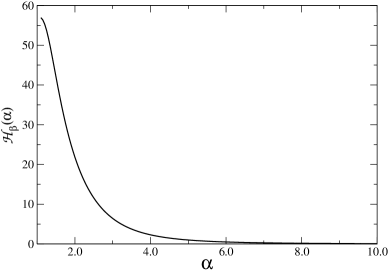
Figure 9: (Color online) Plot of $\mathcal{H}_{\beta}(\alpha)$, which gives a measure of correlation of the two maxima $m_{1}$ and $m_{2}$ for $D_{1}=1.3$ and $D_{2}=1.5$.

If the two maxima $m_{1}$ and $m_{2}$ are independent of each other then the quantity defined above would be identically zero for any $\alpha$ and $L$. We plug the large $L$ expression of $\mathcal{Q}(L,\alpha L|u_{1},u_{2})$ from Eq. (58) and the large $L$ of $\mathcal{Q}_{1}(L|u_{1},u_{2})$ and $\mathcal{Q}_{2}(\alpha L|u_{1},u_{2})$ obtained from Eq. (58) by taking $\alpha\to\infty$ and $\alpha\to 1$ limit, respectively, to see that the function $C_{\theta}(\alpha,L;u_{1},u_{2})$ becomes independent of $L$ [the factor $L^{1/\theta}$ in (60) is chosen for this purpose] and takes the following form

$$C_{\theta}(\alpha,L;u_{1},u_{2})|_{L\to\infty}=\mathcal{H}_{\beta}(\alpha)\mathcal{L}_{\beta}(u_{1},u_{2})\;,$$ (61)

for both processes, where the function $\mathcal{H}_{\beta}(\alpha)$ carries the information on the correlations (the function ${\cal L}_{\beta}(u_{1},u_{2})$ can also be computed explicitly but we do not discuss it here). This function $\mathcal{H}_{\beta}(\alpha)$ is given by

$$\mathcal{H}_{\beta}(\alpha) = \frac{1}{\pi}\left[\left(\pi\tan(\beta)\right)^{\frac{1}{\theta}}+\alpha^{-\frac{1}{\theta}}\left(\frac{\sqrt{\pi}\Gamma[\theta]}{\Gamma[\frac{1}{2}+\theta]}\right)^{\frac{1}{\theta}}-\left(\frac{k_{\theta}(a)\sqrt{a}}{\alpha}\right)^{\frac{1}{\theta}}\right],$$

with $$\theta=\frac{1}{2}-\frac{\beta}{\pi}~{}~{}\text{and}~{}~{}\beta=\arctan\left(\frac{\sqrt{D_{1}}}{\sqrt{D_{2}}}\right).$$ (62)

Here we should keep in mind that according to Eq. (30), $a$ is a function of $\alpha$ and $\beta$. In Fig. 9, we plot $\mathcal{H}_{\beta}(\alpha)$ as a function of $\alpha$ for $D_{1}=1.3$ and $D_{2}=1.5$. This shows that even when both $m_{1},m_{2}$ are large, $m_{1}$ and $m_{2}$ are strongly correlated as long as they are of the same order of magnitude. As expected, these correlations vanish when the two particles are very far away from each other.

3 Multi-particle problem: $N>2$

In this section we generalize the two vicious walkers problem to $N$ vicious walkers problem. We focus on the PDF $p_{N}(m|{\bf u})$ of the global maximum $m_{N}$ (maximal distance travelled by the rightmost particle). Moreover, we assume that the $N$ walkers are identical i..e. they have the same diffusion constant $D_{1}=D_{2}=...=D_{N}=D$. In this case, we expect that the PDF $p_{N}(m|{\bf u})$ will not depend on $D$ and will have the following power law tail

$$p_{N}(m|{\bf u})\simeq\dfrac{\mathcal{A}_{N}({\bf u})}{m^{\nu_{N}}}~{}~{}\text{with}~{}\nu_{N}=N^{2}+1,$$ (63)

for both processes 1 and 2. We first show from a heuristic scaling argument that one can predict the power law in the above equation. The scaling argument is based on the large time tail of the distribution $f_{N}(t_{s}|{\bf u})$ of the stopping time $t_{s}$. This argument provides the $N$-dependence of the exponent $\nu_{N}$ accurately but it does not predict the prefactor precisely. For this we study the $N$-particle problem rigorously in the next subsection, where we follow an approach different from what we have done for the $N=2$ case. In particular, we have used the Green’s function approach directly rather than solving a $N$-dimensional Laplace’s equation inside an $N$-dimensional complicated Weyl chamber because the later approach becomes difficult as we do not have at our disposal any generalized Schwarz-Christoffel transformation valid in dimensions $d>2$.

3.1 A heuristic argument for $N$ particles

To justify the power law for $p_{N}(m|{\bf u})$ given in Eq. (63), we present a simple scaling argument which is based on the power law tail of the PDF of the stopping time $t_{s}$ itself. This argument is valid for both process 1 and process 2 and it goes as follows. Let $Q_{N}(L|{\bf{u}})=\text{Prob.}[m_{N}\leq L|{\bf{u}}]$ be the probability that the global maximum $m_{N}$ stays below the level $L$ given that the $N$ walkers starting from positions ${\bf{u}}$ stay non-intersecting till time $t_{s}$. For large $L$, the dominant contribution to $1-Q_{N}(L|{\bf{u}})=\text{Prob.}[m_{N}\geq L|{\bf{u}}]$ comes from trajectories which typically have large global maximum $m_{N}$. On the other hand, using the connection between non-intersecting Brownian motions and random matrix theory (RMT) one can argue that the average value of the global maximum $m_{N}$ over the time interval $[0,t_{s}]$ grows as $\langle m_{N}\rangle\sim\sqrt{t_{s}~{}N}$, whereas the fluctuations of $m_{N}$ around this mean value decays as $N^{-1/6}$ Schehr08 ; Forrester08 . As a result, the distribution of $m_{N}$ over the time interval $[0,t_{s}]$ will be highly peaked around $m_{N}\sim\sqrt{t_{s}N}$ for very large $N$. Therefore one expects that for large $t_{s}$ and $N$, the random variable $m_{N}$ will be typically of the order of $\sim\sqrt{t_{s}~{}N}$. Hence, for large $N$ and $L$, the tail of the cumulative distribution $Q_{N}(L|{\bf{u}})$ is obtained from :

$$1-Q_{N}(L|{\bf{u}}) = \text{Prob.}[m_{N}>L|{\bf{u}}]\approx\text{Prob.}\left[t_{s}>c\frac{L^{2}}{N}\big{|}{\bf{u}}\right],$$ (64)

$$\text{with}, \text{Prob.}[t_{s}>t|{\bf{u}}]=\int_{t}^{\infty}f_{N}(t^{\prime}|{\bf{u}})dt^{\prime}\;,$$ (65)

where $f_{N}(t_{s}|{\bf{u}})$ is the PDF of the stopping time $t_{s}$ (and $c$ is an undetermined constant, irrelevant for the present argument).

To find the PDF of the “stopping time” $f_{N}(t|{\bf{u}})$ for identical walkers i.e. for $D_{1}=D_{2}=...=D_{N}=D$, we start with the Green’s function $G_{N}({\bf{y}},t;{\bf{u}},0)$ of $N$ non-intersecting Brownian walkers with an absorbing wall at the origin. This Green’s function represents the probability density of the positions ${\bf{y}}=(y_{1},y_{2},...,y_{N})$ of the $N$ walkers at time $t$ given that they had started from positions ${\bf{u}}=(u_{1},u_{2},...,u_{N})$ initially. Using the Karlin-McGregor formula karlin , this $N$-particle Green’s function can be expressed as the determinant of a $N\times N$ matrix $[G_{i,j}]\equiv[g(u_{i},y_{j},t)]$ where

$$g(u,y,t)=\frac{1}{\sqrt{4\pi Dt}}\left(\text{exp}\left[-\frac{(y-u)^{2}}{4Dt}\right]-\text{exp}\left[-\frac{(y+u)^{2}}{4Dt}\right]\right)$$ (66)

is the single particle Green’s function with an absorbing wall at the origin. One can also map the problem of finding $G_{N}({\bf{y}},t;{\bf{u}},0)$ to the problem of finding the wave function of $N$ free fermions with an infinite wall at the origin and this mapping allows us to write Schehr08

$$G_{N}({\bf{y}},t|{\bf{u}},0)=\frac{1}{(\sqrt{2Dt})^{N}}\frac{1}{N!}\left(\frac{2}{\pi}\right)^{N}\int_{0}^{\infty}\dots\int_{0}^{\infty}dq_{1}dq_{2}\dots dq_{N}~{}\Phi_{{\bf{q}}}^{(N)}\left(\frac{{\bf{u}}}{\sqrt{2Dt}}\right)\Phi_{{\bf{q}}}^{(N)}\left(\frac{{\bf{y}}}{\sqrt{2Dt}}\right)e^{-\frac{1}{2}{\bf{q}}^{2}}\;,$$ (67)

where ${\bf{q}}\equiv\{q_{1},q_{2},\dots,q_{N}\}$, ${\bf q}^{2}=\sum_{i=1}^{N}q_{i}^{2}$ and

$$\Phi_{{\bf{q}}}^{(N)}\left({\bf{u}}\right)=\left|\begin{matrix}\sin\left(q_{1}u_{1}\right)&\sin\left(q_{1}u_{2}\right)&\cdots&\sin\left(q_{1}u_{N}\right)\\ \sin\left(q_{2}u_{1}\right)&\sin\left(q_{2}u_{2}\right)&\cdots&\sin\left(q_{2}u_{N}\right)\\ \vdots&\vdots&\ddots&\vdots\\ \sin\left(q_{N}u_{1}\right)&\sin\left(q_{N}u_{2}\right)&\cdots&\sin\left(q_{N}u_{N}\right)\end{matrix}\;\right|.$$ (68)

In case of process 1, the motion of the $N$ walkers “stop” when either any two particles meet each other for the first time before the leftmost particle hits the origin or the first particle crosses the origin for the first time before any two particles meet each other. The survival probability $S_{N}\left(t|{\bf{u}}\right)$ of such $N$-particle process, is given by

$$S_{N}\left(t|{\bf{u}}\right)=\int_{\mathcal{W}}d^{N}{\bf{y}}~{}G_{N}({\bf{y}},t|{\bf{u}},0).$$ (69)

The Weyl chamber $\mathcal{W}$ in the above expression is defined as $\mathcal{W}=[{\bf y}\in\mathbb{R}_{+}^{N}|0\leq y_{1}\leq y_{2}\leq\dots\leq y_{N}\leq\infty]$ where $\mathbb{R}_{+}$ is the set of non-negative real numbers. Hence, for process 1, the PDF of the “stopping time” is

$$f_{N}(t|{\bf{u}})=-\frac{\partial S_{N}\left(t|{\bf{u}}\right)}{\partial t}=-\frac{\partial}{\partial t}\left(~{}\int_{\mathcal{W}}dy_{1}dy_{2}\dots dy_{N}~{}G_{N}({\bf{y}},t|{\bf{u}},0)\right)~{}~{}~{}~{}\text{for~{}process 1}.$$ (70)

On the other hand, for process 2 the reasoning is a bit different as the process gets “stopped” only when the first particle hits the origin for the first time before any two other particles collide. This implies that the PDF $f_{N}(t|{\bf{x}})$ of the “stopping time” is obtained from the outward flux through the $y_{1}=0$ hyperplane $\widetilde{\mathcal{W}}=[{\bf y}\in\mathcal{W}~{}|~{}y_{1}=0]$ of the Weyl chamber $\mathcal{W}$. Hence integrating the outward probability current density $D\left(\frac{\partial G_{N}({\bf{y}},t|{\bf{u}},0)}{\partial y_{1}}\right)_{y_{1}=0}$ over the hyperplane $\widetilde{\mathcal{W}}$ we get

$$f_{N}(t|{\bf{u}})=D\int_{\widetilde{\mathcal{W}}}dy_{2}dy_{3}\dots dy_{N}\left(\frac{\partial G_{N}({\bf{y}},t|{\bf{u}},0)}{\partial y_{1}}\right)_{y_{1}=0}~{}~{}~{}~{}\text{for~{}process 2},$$ (71)

where the Green’s function is explicitly given in Eq. (67).

To obtain the tail of the PDF $f_{N}(t|{\bf{u}})$, we need to find the large $t$ behavior of $G_{N}({\bf{y}},t|{\bf{u}},0)$, which can be obtained by expanding the function $\Phi_{{\bf{q}}}^{(N)}\left(\frac{{\bf{u}}}{\sqrt{t}}\right)$ in Eq. (68) for large $t$ and finite ${\bf u}$. One can show Kobayashi that for large $t$ and finite ${\bf u}$,

$$\Phi_{{\bf{q}}}^{(N)}\left(\frac{{\bf{u}}}{\sqrt{2Dt}}\right)=\det\limits_{1\leq i,j\leq N}\sin\left[q_{i}\frac{u_{j}}{\sqrt{2Dt}}\right]\approx\gamma_{N}~{}\mathcal{Y}_{N}({\bf{q}})~{}\mathcal{Y}_{N}({\bf{u}})~{}\frac{1}{\left(\sqrt{2Dt}~{}\right)^{N^{2}}}+\mathcal{O}\left(t^{-(N^{2}+1)/2}\right),$$ (72)

$$~{}~{}~{}~{}~{}~{}~{}~{}~{}~{}\text{where},~{}~{}~{}~{}\gamma_{N}=\frac{(-1)^{\frac{N(N-1)}{2}}}{\prod\limits_{i=1}^{N}(2i-1)!}~{}~{}~{}~{}~{}~{}~{}\text{and}~{}~{}~{}~{}~{}~{}~{}\mathcal{Y}_{N}({\bf{u}})=\prod_{i=1}^{N}u_{i}\;\prod_{1\leq i<j\leq N}(u_{j}^{2}-u_{i}^{2}).$$ (73)

Plugging the above large $t$ approximation (72) into Eq. (67) and performing the integrations over the variables $q_{i}$, we get

$$G_{N}({\bf{y}},t|{\bf{u}},0)\simeq\frac{\mathcal{Y}_{N}({\bf u})}{(\sqrt{2Dt})^{N^{2}}}~{}\left[\frac{\left(\frac{2}{\pi}\right)^{\frac{N}{2}}}{\prod\limits_{i=1}^{N}(2i-1)!}~{}\frac{1}{(\sqrt{2Dt})^{N}}~{}\text{exp}\left[-\frac{{\bf y}^{2}}{4Dt}\right]~{}\mathcal{Y}_{N}\left(\frac{{\bf y}}{\sqrt{2Dt}}\right)\right].$$ (74)

Finally, putting this large $t$ form of $G_{N}({\bf{y}},t|{\bf{u}},0)$ into Eqs. (70) and (71) and performing the rest of the integrations over the variables $y_{i}$, we obtain

$$f_{N}(t_{s}|{\bf{u}})\sim D\delta_{N}\frac{\mathcal{Y}_{N}({\bf{u}})}{(Dt_{s})^{\zeta}},\;\;\text{with}\;\zeta=\frac{N^{2}}{2}+1,$$ (75)

for both process 1 and process 2, where $\delta_{N}$ is an $N$ dependent constant different for process 1 and process 2. The explicit expressions of $\delta_{N}$ for both processes are given in Appendix A. The above result for $f_{N}(t_{s}|{\bf{u}})$ has also been proved in Krattenthaler ; Bray04 for process 2. Plugging the large $t_{s}$ behavior of $f_{N}(t_{s}|{\bf{u}})$ from Eq. (75) into Eqs. (64) and (65) we get,

$$1-Q_{N}(L|{\bf{u}})\propto B_{N}\mathcal{Y}_{N}({\bf u})/{L^{N^{2}}},~{}\text{for~{}large~{}}L$$ (76)

where, the function $\mathcal{Y}_{N}({\bf u})$ is given in Eq. (73) and $B_{N}$ is an $N$ dependent constant. Upon deriving both sides of the Eq. (76) with respect to $L$ at $L=m$, we get the tail of the PDF $p_{N}(m|{\bf u})$ as given in Eq. (63) with $\nu_{N}=N^{2}+1$ and $\mathcal{A}_{N}=N^{2}B_{N}\mathcal{Y}_{N}({\bf u})$. This heuristic argument also provides a rough estimate of $B_{N}$ for large $N$ and that is $B_{N}\sim\text{exp}\left(\frac{N^{2}}{2}\log N\right)$. Similar scaling arguments have been successfully used to study the distribution of the global maximum $m_{N}$ of $N$ non-interacting particles till their first exit from the half space KrapivskySatya2010 .

This result (76) is in line with the following general results valid for a generic self-affine process. For such a process $x(t)$ starting from $x>0$, the cumulative distribution $Q(L|x)=\text{Prob.}(m\leq L|x)$ of the maximum $m$ till the stopping time $t_{s}$ (time of first passage through $x=0$), or equivalently the exit probability $Q(L|x)$ from the box $[0,L]$ through the origin, has been recently studied in Satyarosso10 where it was shown that $1-Q(L|x)\sim(x/L)^{\phi}$ in the $(x/L)\to 0$ limit. The exponent $\phi$ is related to the persistence exponent $\theta_{p}$ and the Hurst exponent $H$ via the scaling relation $\phi=\theta_{p}/H$ Satyarosso10 . The persistence exponent $\theta_{p}$ characterizes the late time power-law decay of the survival probability, i.e. the probability that the process stays on the positive half-axis up to time $t$ Bray13 ; Satyacurrsci99 , whereas the Hurst exponent characterizes the typical growth of $x(t)\sim t^{H}$ with time $t$. Thus, the PDF of the maximum decays for large $m$ as $P(m|x)\sim m^{-\phi-1}$ with $\phi=\theta_{p}/H$. From Eq. (75) we see that for the multiparticle process the corresponding persistence exponent is $\theta_{p}=\frac{N^{2}}{2}$. If we consider this $N$-particle process as a single self-affine process in $N$-dimensional space with $H=1/2$, then the general argument from Satyarosso10 suggests that $1-Q(L|{\bf x})\sim(1/L)^{\phi}$, with $\phi=(\theta_{p}/H)=N^{2}$, which is in accordance with Eq. (76), although this argument can not predict the precise dependence on the initial positions. In the next subsection we prove $\nu_{N}=N^{2}+1$ on firmer grounds and compute the amplitude exactly.

3.2 The distribution $p_{N}(m|{\bf{u}})$ of the global maximum for $N>2$

Here we study the distribution $p_{N}(m|{\bf{u}})$ of the global maximum $m_{N}$ of $N$ identical (i.e. with identical diffusion constant $D_{1}=D_{2}=...=D_{N}=D$) vicious walkers using the $N$-particle Green’s function. We first compute the cumulative probability $Q_{N}(L|{\bf{u}})=\text{Prob.}(m_{N}\leq L|{\bf{u}})$ which represents the probability that the global maximum $m_{N}$ of the rightmost particle is less or equal to $L$ given that the walkers, starting from positions ${\bf{u}}=(u_{1},u_{2},...,u_{N})$ stayed non-intersecting till the “stopping time” $t_{s}$. Upon taking the derivative of $Q_{N}(L|{\bf{u}})$ with respect to $L$ at $L=m$ we get the PDF $p_{N}(m|{\bf{u}})$. To compute this cumulative probability $Q_{N}(L|{\bf{u}})$ we consider the first exit problem of a single $N$-dimensional Brownian walker ${\bf{u(t)}}=(u_{1}(t),u_{2}(t),...,u_{N}(t))$ from the region $\mathcal{T}_{N}(L)=\{{\bf{u}}\in{\mathbb{R}}_{+}^{N}|0<u_{1}<u_{2}<...<u_{N}<L\}$, as done for the $N=2$-particle case (see Fig. 2). For process 1 we consider the first exit probability of the walker through any of the boundaries $u_{1}=0$ or $u_{i+1}=u_{i}$ with $i=1,2,...,N-1$. These exit events correspond, in the original $N$-particle problem, to the following events: (a) leftmost particle crossing the origin for the first time before any two particles meet or (b) any two particle meet for the first time before the leftmost particle hits the origin. On the other hand for process 2, we consider the first exit probability of the $N$-dimensional walker only through the boundary $u_{1}=0$. This event corresponds to the leftmost particle hitting the origin for the first time before any two particles meet in the $N$-particle picture. We denote this first exit probability for both process 1 and process 2 by $F_{N}({\bf u},L)$. For process 1, one can see that $F_{N}({\bf u},L)$ is equal to the time integration from $t=0$ to $t=\infty$ of the total outward probability flux through all the boundaries of $\mathcal{T}_{N}(L)$ (which is equal to 1) minus time integration of the outward flux through the boundary $u_{N}=L$ whereas for process 2 $F_{N}({\bf u},L)$ is equal to the time integration of the outward flux only through the boundary $u_{1}=0$. Hence, the probability $F_{N}({\bf u},L)$ can be expressed in terms of the Green’s function $G^{(L)}_{N}({\bf y},t~{}|~{}{\bf u},0)$ as,

$$F_{N}({\bf u},L) = 1+D\int\limits_{0}^{\infty}dt\int_{W_{0}^{L}}d^{N-1}{\bf{y}}\left(\frac{\partial G_{N}^{(L)}}{\partial y_{N}}\right)_{y_{N}=L}~{}~{}~{}~{}\text{for~{}process~{}1}$$ (77)

$$\text{and}~{}~{}~{}F_{N}({\bf u},L) = ~{}~{}~{}~{}~{}D\int\limits_{0}^{\infty}dt\int_{W_{0}^{L}}d^{N-1}{\bf{y}}\left(\frac{\partial G_{N}^{(L)}}{\partial y_{1}}\right)_{y_{1}=0}~{}~{}~{}~{}\;\,\text{for~{}process~{}2},$$ (78)

where, we have introduced the notations

$$\int_{W_{a}^{b}}d^{N-1}{\bf{y}} = \int\limits_{a}^{b}dy_{N-1}\int\limits_{a}^{y_{N-1}}dy_{N-2}...\int\limits_{a}^{y_{2}}dy_{1}~{}~{}~{}~{}~{}\text{for~{}process~{}1},$$ (79)

$$\text{and}~{}~{}~{}\int_{W_{a}^{b}}d^{N-1}{\bf{y}} = \int\limits_{a}^{b}dy_{N}\int\limits_{a}^{y_{N}}dy_{N-1}...\int\limits_{a}^{y_{3}}dy_{2}~{}~{}~{}~{}~{}~{}~{}~{}~{}~{}~{}\text{for~{}process~{}2}.$$ (80)

The Green’s function used in Eqs. (77) and (78) represents the probability density that $N$ non-intersecting Brownian walkers, starting initially from ${\bf u}$, reach ${\bf y}$ in time $t$ . From Karlin-McGregor formula karlin , it can be written in terms of a determinant of single particle propagators inside a box $[0,L]$ as,

$$G^{(L)}_{N}({\bf y},t~{}|~{}{\bf u},0)=\det\limits_{1\leq i,j\leq N}\left[\sum\limits_{m=-\infty}^{\infty}g(u_{i},y_{j}+2mL,t)\right],$$ (81)

where the function $g(u,y,t)$ is given in Eq. (66). Putting this form of the Green’s function in Eqs. (77) and (78), one can see that $F_{N}({\bf u},L)$ can be expressed for both process 1 and process 2 as

$$F_{N}({\bf u},L)=\sum\limits_{\{{\bf{m}}\}}\mathcal{J}_{{\bf m}}^{(N)}({\bf u},L)~{}~{}\text{where}~{}~{}~{}\sum\limits_{\{{\bf{m}}\}}\equiv\sum\limits_{m_{1}=-\infty}^{\infty}\sum\limits_{m_{2}=-\infty}^{\infty}...\sum\limits_{m_{N}=-\infty}^{\infty}\;,$$ (82)

and

$$\mathcal{J}_{{\bf m}}^{(N)}({\bf u},L)=\delta_{{\bf m,0}}+D\int\limits_{0}^{\infty}dt\int_{W_{0}^{L}}d^{N-1}{\bf{y}}\left(\frac{\partial}{\partial y_{N}}\det\limits_{1\leq i,j\leq N}g(u_{i},y_{j}+2m_{j}L,t)\right)_{y_{N}=L}\text{for~{}process 1}$$ (83)

$$\mathcal{J}_{{\bf m}}^{(N)}({\bf u},L)=~{}~{}~{}~{}~{}~{}~{}~{}~{}~{}D\int\limits_{0}^{\infty}dt\int_{W_{0}^{L}}d^{N-1}{\bf{y}}\left(\frac{\partial}{\partial y_{1}}\det\limits_{1\leq i,j\leq N}g(u_{i},y_{j}+2m_{j}L,t)\right)_{y_{1}=0}\;\;\text{for~{}process 2}\;.$$ (84)

We will see later that the above form of $F_{N}({\bf u},L)$ in Eq. (82) will be convenient to compute the large $L$ asymptotics which will be needed to compute the tail of the PDF $p_{N}(m|{\bf u})$ [see Eq. (63)]. Once we know $F_{N}({\bf u},L)$, the cumulative probability $Q_{N}(L|{\bf{u}})$ is obtained from the ratio (as done in the $N=2$-particle case)

$$Q_{N}(L|{\bf{u}})=\frac{F({\bf{u}},L)}{S_{N}({\bf u})},\;\;\;\text{where}~{}~{}S_{N}({\bf u})=\lim\limits_{L\to\infty}F({\bf{u}},L)\;.$$ (85)

This ratio represents the fraction of such group of $N$ Brownian trajectories starting from positions ${\bf u}=(u_{1},u_{2},...,u_{N})$, which have global maximum $m_{N}\leq L$ and stay mutually non-intersecting till the stopping time $t_{s}$. In the denominator, the quantity $S_{N}({\bf u})$ in Eq. (85) represents the probability that the process will “stop” ultimately. Clearly, for process 1 this probability is exactly one whereas for process 2 this probability is smaller than one ($S_{N}({\bf u})<1$) and expressed as

$$S_{N}({\bf u})=D\frac{1}{N!}\left(\frac{2}{\pi}\right)^{N}\int_{0}^{\infty}d\tau~{}\int_{W_{0}^{\infty}}d^{N-1}{\bf{y}}~{}\int_{0}^{\infty}d^{N}{\bf{k}}~{}~{}\text{exp}\left[-{\bf{k}}^{2}D\tau\right]~{}\Phi_{{\bf{k}}}^{(N)}\left({\bf u}\right)\left\{\frac{\partial}{\partial y_{1}}\Phi_{{\bf k}}^{(N)}\left({\bf{y}}\right)\right\}_{y_{1}=0}$$ (86)

where $\Phi_{{\bf{k}}}^{(N)}\left({\bf u}\right)$ is given in Eq. (68). A more explicit expression of $S_{N}({\bf u})$ is given in Eq. (117). One can, in principle, compute the integral in Eq. (86) for any given $N$ and ${\bf u}\equiv(u_{1},u_{2},....,u_{N})$. For $N=2$, the probability $S_{2}({\bf u})$ is explicitly given by $S_{2}({\bf u})=\frac{4}{\pi}\arctan\left(\frac{u_{2}}{u_{1}}\right)-1$ [see Eq. (15) for $D_{1}=D_{2}$]. For $N=3$, an explicit expression of $S_{3}({\bf u})$ is given in Eq. (119).

To find the large $m$ form of the distribution $p_{N}(m|{\bf{u}})$, we first look at the large $L$ limit of $F({\bf u},L)$ to get the large $L$ form of $Q_{N}(L|{\bf{u}})$ from Eq. (85). We show below in Eq. (95) that, for both process 1 and process 2 the probability $F({\bf u},L)$ has the following large $L$ form

$$F({\bf u},L) = S_{N}({\bf u})-B_{N}\frac{\mathcal{Y}_{N}({\bf{u}})}{L^{N^{2}}}+\mathcal{O}\left(\frac{1}{L^{N^{2}+1}}\right)~{}~{}\text{where,}$$ (87)

$$\mathcal{Y}_{N}({\bf u}) = \prod_{i=1}^{N}u_{i}\;\prod_{1\leq i<j\leq N}(u_{j}^{2}-u_{i}^{2}),$$ (88)

and $B_{N}$ is an $N$ dependent constant. Hence from the ratio in Eq. (85) we get

$$Q_{N}(L|{\bf{u}})=1-B_{N}\frac{\mathcal{Y}_{N}({\bf{u}})}{S_{N}({\bf u})}~{}\frac{1}{L^{N^{2}}}+\mathcal{O}\left(\frac{1}{L^{N^{2}+1}}\right),$$ (89)

from which we finally obtain

$$p_{N}(m|{\bf u})=\left(\frac{\partial Q_{N}(L|{\bf{u}})}{\partial L}\right)_{L=m}\simeq N^{2}B_{N}\frac{\mathcal{Y}_{N}({\bf{u}})}{S_{N}({\bf u})}~{}\frac{1}{m^{(N^{2}+1)}}~{}~{}\text{for}~{}~{}m\gg u_{N},$$ (90)

as announced in Eq. (63). This asymptotic result indicates that for $N$ walkers, integer moments of $m_{N}$ up to order $(N^{2}-1)$ are finite, while higher integer moments are infinite. Therefore as $N$ increases, the distribution becomes narrower and narrower as expected but this happens in a nontrivial way. It is instructive to compare the prefactor of the algebraic tail of $p_{N}(m|{\bf u})$ in Eq. (90) with the same amplitude in the non-interacting case in Eq. (1). Besides the factor $\prod_{i}u_{i}$ which is in common with the non-interacting case, the non-intersecting condition is encoded in this amplitude (90) through the Vandermonde determinant in $\mathcal{Y}_{N}({\bf u})$ (88). The appearance of the Vandermonde determinant is reminiscent of the connection between the present vicious walkers problem and random matrix theory Schehr08 .

In the following we give an outline of the proof of Eqs. (87) and (88) for process 2. For process 1 one can follow similar calculations starting from Eqs. (82) and (83) to arrive at Eq. (87). We start by using the following identity

$$g(u,y,t)=\frac{1}{\sqrt{4\pi Dt}}\left[\text{exp}\left(-\frac{(u-y)^{2}}{4Dt}\right)-\text{exp}\left(-\frac{(u+y)^{2}}{4Dt}\right)\right]=\frac{2}{\pi}\int_{0}^{\infty}dk~{}\sin(ku)\sin(ky)~{}e^{-k^{2}Dt},$$ (91)

in the expression of the Green’s function $g(u,y,t)$ in Eq. (84). By performing then some algebraic manipulations, one can show from Eq. (82) that the first exit probability $F({\bf u},L)$ can be written in the following form

$$F({\bf u},L)=S_{N}({\bf u})+\frac{1}{N!}\left(\frac{2}{\pi}\right)^{N}\sum\limits_{\{{\bf{m}}\}}q_{N}^{({\bf{m}})}({\bf u},L)~{}~{}~{}\text{where},$$ (92)

$$q_{N}^{({\bf{0}})}({\bf u},L)=-D\int_{0}^{\infty}d\tau~{}\int_{W_{1}^{\infty}}d^{N-1}{\bf{z}}~{}\int_{0}^{\infty}d^{N}{\bf{q}}~{}~{}\text{exp}\left[-{\bf{q}}^{2}D\tau\right]~{}\Phi_{{\bf{q}}}^{(N)}\left(\frac{{\bf{u}}}{L}\right)\left\{\frac{\partial}{\partial z_{1}}\Phi_{{\bf{q}}}^{(N)}\left({\bf{z}}\right)\right\}_{z_{1}=0},$$ (93)

$$q_{N}^{({\bf{m}})}({\bf u},L)=D\int_{0}^{\infty}d\tau~{}\int_{W_{0}^{1}}d^{N-1}{\bf{z}}~{}\int_{0}^{\infty}d^{N}{\bf{q}}~{}~{}\text{exp}\left[-{\bf q}^{2}D\tau\right]~{}\Phi_{{\bf{q}}}^{(N)}\left(\frac{{\bf{u}}}{L}\right)\left\{\frac{\partial}{\partial z_{1}}\Phi_{{\bf{q}}}^{(N)}\left({\bf{z}+2{\bf m}}\right)\right\}_{z_{1}=0}$$ (94)

and $S_{N}({\bf u})$ and $\Phi_{{\bf{k}}}^{(N)}\left({\bf u}\right)$ are given in Eqs. (86) and (68) respectively. To arrive at the above expression of $F({\bf u},L)$ we used that $\int_{W_{0}^{L}}d^{N-1}y=\int_{W_{0}^{\infty}}d^{N-1}y-\int_{W_{L}^{\infty}}d^{N-1}y$ and performed the following change of variables ${\bf k}=\frac{{\bf q}}{L}$, ${\bf y}={\bf z}~{}L$ inside the integrations. Note that this expression of $F({\bf u},L)$ given in Eq. (92) is more suitable for obtaining a large $L$ asymptotic as the $L$ dependence is contained in the function $\Phi_{{\bf{q}}}^{(N)}\left(\frac{{\bf{u}}}{L}\right)$ which is a determinant of $\sin\left[q_{i}\frac{u_{j}}{L}\right]$ (68). The large $L$ expansion of $\Phi_{{\bf{q}}}^{(N)}\left(\frac{{\bf{u}}}{L}\right)$ is obtained from Eq. (72) by replacing $t=\frac{L^{2}}{2D}$. Plugging this large $L$ behavior in Eqs. (93) and (94), we get from Eq. (92)

$$F({\bf u},L)=S_{N}({\bf u})-B_{N}\frac{\mathcal{Y}_{N}({\bf{u}})}{L^{N^{2}}}+\mathcal{O}\left(\frac{1}{L^{N^{2}+1}}\right)\;,\;L\to\infty\\$$ (95)

where,

$$~{}~{}~{}~{}B_{N}=r_{N}\left[R_{N}({\bf{0}})-\sum\limits_{\{{\bf{m}\neq{\bf 0}}\}}R_{N}({\bf{m}})\right],~{}~{}\text{with}~{}r_{N}=\frac{(-1)^{\frac{N(N-1)}{2}}}{2N!\prod\limits_{i=1}^{N}(2i-1)!}\left(\frac{2}{\pi}\right)^{N}\;,\;{\rm and}$$ (96)

$$~{}~{}~{}~{}~{}R_{N}({\bf{0}})=\int_{0}^{\infty}d\tau~{}\int_{W_{1}^{\infty}}d^{N-1}{\bf{z}}~{}\int_{0}^{\infty}d^{N}{\bf{q}}~{}~{}\text{exp}\left[-\frac{{\bf q}^{2}\tau}{2}\right]~{}\mathcal{Y}({\bf q})~{}\left\{\frac{\partial}{\partial z_{1}}\Phi_{{\bf{q}}}^{(N)}\left({\bf{z}}\right)\right\}_{z_{1}=0},$$ (97)

$$~{}~{}~{}~{}~{}R_{N}({\bf{m}})=\int_{0}^{\infty}d\tau~{}\int_{W_{0}^{1}}d^{N-1}{\bf{z}}~{}\int_{0}^{\infty}d^{N}{\bf{q}}~{}~{}\text{exp}\left[-\frac{{\bf q}^{2}\tau}{2}\right]~{}\mathcal{Y}({\bf q})~{}\left\{\frac{\partial}{\partial z_{1}}\Phi_{{\bf{q}}}^{(N)}\left({\bf{z}+2{\bf m}}\right)\right\}_{z_{1}=0},$$ (98)

and the function $\mathcal{Y}({\bf q})$ is given in Eq. (88). The integration over the variables $z_{i}$ in the above formula is understood in terms of the notations given in Eq. (80). Moreover one should note that the domain of integration corresponding to the integration over the variables $z_{i}$ in the case ${\bf m}={\bf 0}$ is different from the case ${\bf m}\neq{\bf 0}$. Performing the integrations over $q_{i}$’s in Eqs. (97) and (98), one can rewrite the constant $B_{N}$ given in Eq. (95) as

$$B_{N} = d_{N}\left[h_{N}({\bf{0}})-\sum\limits_{\{{\bf{m}\neq{\bf 0}}\}}h_{N}({\bf{m}})\right],~{}~{}\text{with}~{}~{}~{}d_{N}=\frac{1}{2\prod\limits_{i=1}^{N}(2i-1)!}\left(\frac{2}{\pi}\right)^{\frac{N}{2}},~{}~{}~{}\text{and}~{}$$ (99)

$$h_{N}({\bf{0}}) = \int_{0}^{\infty}d\tau~{}\tau^{-\frac{N(N+1)}{2}}\int_{W_{1}^{\infty}}d^{N-1}{\bf{z}}~{}\text{exp}\left(-\frac{{\bf z}^{2}}{2\tau}\right)\left[\frac{\partial}{\partial z_{1}}\mathcal{Y}_{N}\left(\frac{{\bf z}}{\sqrt{\tau}}\right)\right]_{z_{1}=0}$$

$$h_{N}({\bf{m}}) = \int_{0}^{\infty}d\tau~{}{\tau^{-\frac{N(N+1)}{2}}}\int_{W_{0}^{1}}d^{N-1}{\bf{z}}~{}\left[\frac{\partial}{\partial z_{1}}~{}\text{exp}\left(-\frac{({\bf{z}}+2{\bf{m}})^{2}}{2\tau}\right)\mathcal{Y}_{N}\left(\frac{{\bf{z}}+2{\bf{m}}}{\sqrt{\tau}}\right)\right]_{z_{1}=0},$$ (100)

where, again, the function $\mathcal{Y}_{N}({\bf u})$ is given in Eq. (88). In principle one can compute numerically the constant $B_{N}$ given in Eq. (99) for any given $N$. For instance, for $N=2$, such a numerical evaluation yields $B_{2}=2.25689\ldots$. Comparing the expression of $p_{2}(m|{\bf u})$ in Eq. (90) for $N=2$ with the Eq. (56), we see that the value of $B_{2}$ obtained from the Green’s function method matches exactly with the value of $k_{2}/4=\frac{3~{}\Gamma[1/4]^{8}}{20(4\pi)^{3}}=2.25689\ldots$ obtained previously in Eq. (57) for process 2 through a completely different approach (using Schwarz-Christoffel mapping). For $N=3$ we obtain the numerical estimate from (99) $B_{3}=16.3053..$. It is interesting to find the large $N$ asymptotic behavior of $B_{N}$. One can argue and we have checked it numerically with Mathematica that for large $N$ the dominant contribution to $B_{N}$ in Eq. (99) comes from the term $h_{N}(0,0,..,0,-1)$. Hence we conjecture that

$$B_{N}\simeq d_{N}\Delta_{N}\,~{}~{}\text{for~{}large}~{}N,~{}~{}\text{where}~{}\Delta_{N}=-h_{N}(0,0,...,0,-1),$$ (101)

and $d_{N}$ is given in Eq. (99). From Eq. (100), one can see that $\Delta_{N}$ has the following form

$$\Delta_{N}=\int_{0}^{\infty}d\tau~{}{\tau^{-\frac{N^{2}+N+4}{2}}}\int_{0}^{1}dz_{N}~{}\text{exp}\left[-\frac{(z_{N}-2)^{2}}{2\tau}\right]~{}(2-z_{N})^{3}~{}\mathcal{K}_{N-2}(z_{N},\tau),$$ (102)

where the explicit expression of the function $\mathcal{K}_{N}(x,\tau)$ is given in Eq. (122) (see Appendix D). The large $N$ analysis of $\mathcal{K}_{N}(x,\tau)$ can be carried out using analytical techniques from random matrix theory, namely Coulomb gas techniques Dyson ; Dean08 ; Dean08II ; Bohigas (for a review see Ref. Majumdar14 ). We then show in Appendix D that for large $N\gg 1$, the constant $\Delta_{N}$ grows as :

$$\Delta_{N}=-h_{N}(0,0,...,0,-1)\approx\text{exp}\left(\frac{3N^{2}}{2}\log N\right).$$ (103)

On the other hand, from the explicit expression of $d_{N}$ given in Eq. (99) we get

$$d_{N}\approx\text{exp}\left(-\frac{N^{2}}{2}\log N\right),~{}~{}\text{for}~{}~{}N\gg 1\;.$$ (104)

Hence using Eqs. (103) and (104) in Eq. (101) we finally get

$$B_{N}\simeq d_{N}\Delta_{N}\approx\text{exp}\left(\frac{N^{2}}{2}[\log N+o(\log N)]\right)~{}~{}\text{for}~{}~{}N\gg 1\;,$$ (105)

where $o(\log N)$ represents terms smaller than $\log N$. This large $N$ asymptotic form of $B_{N}$ agrees with the rough estimate obtained from the heuristic argument in section 3.1.

4 Conclusion

To summarize, we have considered the extreme statistics of $N$ non-intersecting Brownian motions in one dimension (“vicious walkers”), till their survival. These Brownian particles “survive” over a random time interval $[0,t_{s}]$ where $t_{s}$ is usually called the “stopping time”. We consider two different stopping mechanisms named process 1 and process 2 to define $t_{s}$. For process 1, the $N$-particle process gets “stopped” when either any of the two particles among $N$ particles meet each other for the first time before the leftmost one hits the origin or the leftmost particle hits the origin for the first time before any two particles meet each other (see Fig. 1). On the other hand, for process 2, the “stopping time” $t_{s}$ is determined from the first passage time of the leftmost walker given that no other two particles have met before $t_{s}$. For $N=2$ particles, we have computed exactly the joint cumulative distribution function $\mathcal{Q}(L_{1},L_{2}|u_{1},u_{2})$ of the maxima of the leftmost and rightmost particle till their survival. This was done by solving a two-dimensional backward Fokker-Planck equation with the help of a conformal mapping, namely the Schwarz-Christoffel transformation. From the joint cumulative distribution we have obtained the marginal PDFs of the maxima of the first and second particle $p_{1}(m|u_{1},u_{2})$ and $p_{2}(m|u_{1},u_{2})$ respectively. For general $N$ identical walkers, we have computed the tail of the distribution $p_{N}(m|{\bf u})$ of the global maximum $m_{N}$ in two ways. The first one is using a heuristic argument based on the distribution $f_{N}(t|{\bf u})$ of the “stopping time” while the second one is an exact calculation based on $N$-particle Green’s function.

This work raises several interesting questions, which certainly deserve further studies. The first extension of the present study is the computation of the exponent $\nu_{N}$ and the associated amplitude $\mathcal{A}_{N}(\bf{u},\bf{D})$ for $N>2$ particles and different diffusion constants. This is a challenging question from a technical point of view as, in this case, one can not use the Karlin-McGregor formula. In this paper, we have mostly focused on the distribution of the value of the global maximum $m_{N}$ of $N$ non-intersecting walkers till the stopping time $t_{s}$. Another interesting observable is not just the actual value of the maximum $m_{N}$, but the time $t_{m}$ at which this maximum occurs before the stopping time $t_{s}$. The PDF of $t_{m}$ was studied for vicious walkers over a fixed time interval Rambeau11 , with interesting application to stochastic growth processes Rambeau10 , and it will be interesting to study it for the stopped multi-particle process. Finally, another interesting open question concerns the distribution $p_{1}(m|{\bf u})$ of the maximum displacement $m_{1}$ of the leftmost walker for $N>2$. This is an interesting quantity as the maximal displacement $m_{1}$ travelled by the leftmost particle can be considered, for instance, as a measure of the common region Anupam13 visited by all the walkers.

Appendix A The constant $\delta_{N}$ in Eq. (75)

Here we give explicit and exact expression of the constant $\delta_{N}$ appearing in Eq. (75) for both processes 1 and 2.
For process 1

$$\delta_{N} = \frac{\left(\frac{2}{\pi}\right)^{N/2}N^{2}}{2^{(\frac{N^{2}}{2}+1)}\prod\limits_{j=1}^{N}\Gamma[2i]}\int\limits_{0}^{\infty}dz_{N}\int\limits_{0}^{z_{N}}dz_{N-1}...\int\limits_{0}^{z_{3}}dz_{2}\int\limits_{0}^{z_{2}}dz_{1}\;\text{exp}\left(-\sum\limits_{i=1}^{N}\frac{z_{i}^{2}}{2}\right)\prod\limits_{i=1}^{N}z_{i}\prod_{1\leq i<j\leq N}(z_{j}^{2}-z_{i}^{2})$$ (106)

$$= ~{}~{}~{}~{}~{}~{}~{}~{}~{}~{}~{}~{}\left(\frac{2}{\pi}\right)^{N}\frac{N}{2(N-1)!}~{}\frac{\prod\limits_{j=1}^{N}\Gamma\left[1+\frac{j}{2}\right]\Gamma\left[1+\frac{j-1}{2}\right]}{\prod\limits_{i=1}^{N}\Gamma[2i]},~{}~{}~{}~{}\text{and}$$

for process 2

$$\delta_{N} = \frac{\left(\frac{2}{\pi}\right)^{N/2}}{2^{(\frac{N^{2}}{2}+1)}\prod\limits_{j=1}^{N}\Gamma[2i]}\int\limits_{0}^{\infty}dz_{N}\int\limits_{0}^{z_{N}}dz_{N-1}...\int\limits_{0}^{z_{3}}dz_{2}\text{exp}\left(-\sum\limits_{i=2}^{N}\frac{z_{i}^{2}}{2}\right)\prod\limits_{i=2}^{N}z_{i}^{3}\prod_{2\leq i<j\leq N}(z_{j}^{2}-z_{i}^{2})$$ (107)

$$= ~{}~{}~{}~{}~{}~{}~{}~{}~{}~{}~{}~{}\left(\frac{2}{\pi}\right)^{N}\frac{N\sqrt{\pi}}{8~{}N!}~{}\frac{\prod\limits_{j=1}^{N-1}\Gamma\left[1+\frac{j}{2}\right]\Gamma\left[2+\frac{j-1}{2}\right]}{\prod\limits_{i=1}^{N}\Gamma[2i]}$$

where $\Gamma[x]$ is the Gamma function. These two expressions are obtained using exact formulas for Selberg integrals Mehta .

Appendix B Explicit expressions of the functions $\mathcal{B}(u_{1},u_{2},\alpha,\mu)$ and $\mathcal{A}_{i}(u_{1},u_{2},\mu)$.

Following the method explained in section 2, one can compute the joint cumulative distribution function of $m_{1}$ and $m_{2}$ till the stopping time $t_{s}$ for any diffusion coefficients $D_{1},D_{2}$. We will not give the details here but only quote the results for the asymptotic behaviors which one can extract from this exact calculation. One finds indeed

$$\mathcal{Q}(L,\alpha L|u_{1},u_{2})\approx 1-\frac{\mathcal{B}(u_{1},u_{2},\alpha,\mu)}{L^{\mu}}~{}~{}\text{with}~{}~{}\mu=\frac{2\pi}{\pi-2\arctan\left(\sqrt{\frac{D_{1}}{D_{2}}}\right)}~{}~{}~{}\text{for}~{}~{}L\gg u_{2}$$ (108)

$$\mathcal{B}(u_{1},u_{2},\alpha,\mu) = \frac{1}{\pi}\mathcal{X}_{\theta}(a)~{}\left(\sqrt{\frac{D_{2}u_{1}^{2}+D_{1}u_{2}^{2}}{D_{2}}}\right)^{\frac{1}{\theta}}~{}\sin\left(\frac{\psi-\beta}{\theta}\right)~{}~{}~{}~{}\text{for process 1 and }$$ (109)

$$\mathcal{B}(u_{1},u_{2},\alpha,\mu) = \frac{\theta}{\psi-\beta}\left(\frac{2a\theta+a-1}{2a(1+\theta)}\right)\mathcal{X}_{\theta}(a)~{}\left(\sqrt{\frac{D_{2}u_{1}^{2}+D_{1}u_{2}^{2}}{D_{2}}}\right)^{\frac{1}{\theta}}~{}\sin\left(\frac{\psi-\beta}{\theta}\right)~{}~{}~{}~{}\text{for process 2}$$ (110)

$$\text{where},~{}\mathcal{X}_{\theta}(a) = \left(\theta~{}h_{\theta}(a)\sqrt{a}\right)^{\frac{1}{\theta}},~{}\psi=\arctan\left(\frac{\sqrt{D_{1}}u_{2}}{\sqrt{D_{2}}u_{1}}\right),~{}~{}\theta=\frac{1}{2}-\frac{\beta}{\pi}~{}~{}\text{with}~{}~{}\beta=\arctan\left(\sqrt{\frac{D_{1}}{D_{2}}}\right),$$ (111)

which yields the asymptotic behaviors of the PDFs:

$$p_{i}(m|u_{1},u_{2})\approx\frac{\mathcal{A}_{i}(u_{1},u_{2},\mu)}{m^{\nu}}~{}~{}\text{with}~{}~{}\nu=\mu+1~{}~{}~{}\text{for}~{}~{}m\gg u_{2}\;~{}\text{and}~{}i=1,2.$$ (112)

The amplitudes $\mathcal{A}_{i}(u_{1},u_{2},\mu)$ are explicitly given by

$$\mathcal{A}_{1}(u_{1},u_{2},\mu) = \frac{1}{\pi\theta}\left(\frac{\pi\theta\sqrt{D_{2}u_{1}^{2}+D_{1}u_{2}^{2}}}{\sqrt{D_{2}}}\right)^{\frac{1}{\theta}}~{}\sin\left(\left[\arctan\left(\frac{\sqrt{D_{1}}u_{2}}{\sqrt{D_{2}}u_{1}}\right)-\beta\right]\theta^{-1}\right)~{}~{}{\text{process 1}}$$ (113)

$$\mathcal{A}_{1}(u_{1},u_{2},\mu) = \left(\frac{\theta}{1+\theta}\right)\left(\frac{\pi\theta\sqrt{D_{2}u_{1}^{2}+D_{1}u_{2}^{2}}}{\sqrt{D_{2}}}\right)^{\frac{1}{\theta}}\frac{\sin\left(\left[\arctan\left(\frac{\sqrt{D_{1}}u_{2}}{\sqrt{D_{2}}u_{1}}\right)-\beta\right]\theta^{-1}\right)}{\left[\arctan\left(\frac{\sqrt{D_{1}}u_{2}}{\sqrt{D_{2}}u_{1}}\right)-\beta\right]}~{}~{}{\text{process 2}}\;,~{}$$ (114)

together with

$$\mathcal{A}_{2}(u_{1},u_{2},\mu) = \frac{1}{\pi\theta}\left(\frac{\theta~{}\Gamma[\theta]\Gamma[\frac{1}{2}-\theta]\sqrt{D_{2}u_{1}^{2}+D_{1}u_{2}^{2}}}{\sqrt{\pi}\sqrt{D_{1}+D_{2}}}\right)^{\frac{1}{\theta}}~{}\sin\left(\left[\arctan\left(\frac{\sqrt{D_{1}}u_{2}}{\sqrt{D_{2}}u_{1}}\right)-\beta\right]\theta^{-1}\right)\,{\text{process 1}}$$ (115)

$$\mathcal{A}_{2}(u_{1},u_{2},\mu) = \left(\frac{1+2\theta}{2(1+\theta)}\right)\left(\frac{\theta~{}\Gamma[\theta]\Gamma[\frac{1}{2}-\theta]\sqrt{D_{2}u_{1}^{2}+D_{1}u_{2}^{2}}}{\sqrt{\pi}\sqrt{D_{1}+D_{2}}}\right)^{\frac{1}{\theta}}\frac{\sin\left(\left[\arctan\left(\frac{\sqrt{D_{1}}u_{2}}{\sqrt{D_{2}}u_{1}}\right)-\beta\right]\theta^{-1}\right)}{\left[\arctan\left(\frac{\sqrt{D_{1}}u_{2}}{\sqrt{D_{2}}u_{1}}\right)-\beta\right]}\,{\text{process 2}}\;.$$

(116)

Appendix C The exit probability $S_{N}({\bf u})$ given in Eq. (86)

After performing the integrations over $k_{i}$ variables in Eq. (86), the exit probability $S_{N}({\bf u})$ can be rewritten as

$$S_{N}({\bf u})=\frac{4}{\sqrt{\pi}}\sum\limits_{i=1}^{N}(-1)^{i+1}\int\limits_{0}^{\infty}dt~{}\frac{u_{i}}{\sqrt{4t}}~{}\text{exp}\left(-\frac{u_{i}^{2}}{4t}\right)\int\limits_{0}^{\infty}dz_{N}\int\limits_{0}^{z_{N}}dz_{N-1}...\int\limits_{0}^{z_{3}}dz_{2}~{}~{}\det\left[\bm{\tilde{\Lambda}}_{i}\left(\frac{{\bf u}}{\sqrt{4t}};z_{2},z_{3},...,z_{N}\right)\right]\;,$$ (117)

where $\bm{\tilde{\Lambda}}_{i}$ is an $(N-1)\times(N-1)$ matrix obtained by removing the $i^{\text{th}}$ row and $1^{\text{st}}$ column from the $N\times N$ matrix $\bm{\tilde{\Lambda}}$ whose elements are given by $[\bm{\tilde{\Lambda}}]_{i,j}=\sqrt{\pi}g\left(\frac{u_{i}}{\sqrt{4t}},z_{j},\frac{1}{4D}\right)$. We recall that the function $g\left(u,y,t\right)$ is given by

$$g(u,y,t)=\frac{1}{\sqrt{4\pi Dt}}\left(\text{exp}\left[-\frac{(y-u)^{2}}{4Dt}\right]-\text{exp}\left[-\frac{(y+u)^{2}}{4Dt}\right]\right).$$ (118)

For $N=3$ we can obtain an explicit expression for the exit probability $S_{3}({\bf u})$. It is given by

$$S_{3}(u_{1},u_{2},u_{3})= \left\{\Psi(u_{1},u_{2},u_{3})-\Psi(u_{1},u_{3},u_{2})\right\}+\left\{\Psi(u_{2},u_{3},u_{1})-\Psi(u_{2},u_{1},u_{3})\right\}$$ (119)

$$~{}~{}~{}~{}~{}~{}~{}~{}~{}~{}~{}~{}~{}~{}~{}+\left\{\Psi(u_{3},u_{1},u_{2})-\Psi(u_{3},u_{2},u_{1})\right\}$$

where

$$\Psi(x,y,z)=\frac{x}{\pi}\Bigg{[}$$ (120)

$$\text{ArcTan}\left(\frac{x\left(\sqrt{x^{2}+y^{2}+z^{2}}+y-z\right)}{x^{2}+\sqrt{\left(2x^{2}+(y+z)^{2}\right)\left(2z\left(z-\sqrt{x^{2}+y^{2}+z^{2}}\right)+x^{2}+y^{2}\right)}-(y+z)\left(\sqrt{x^{2}+y^{2}+z^{2}}-z\right)}\right)$$

$$-\text{ArcTan}\left(\frac{x\left(\sqrt{x^{2}+y^{2}+z^{2}}-y-z\right)}{x^{2}+\sqrt{\left(2x^{2}+(y+z)^{2}\right)\left(2z\left(z-\sqrt{x^{2}+y^{2}+z^{2}}\right)+x^{2}+y^{2}\right)}+(y+z)\left(\sqrt{x^{2}+y^{2}+z^{2}}-z\right)}\right)\allowdisplaybreaks[4]$$

$$-\text{ArcTan}\left(\frac{x\left(\sqrt{x^{2}+y^{2}+z^{2}}+y+z\right)}{x^{2}+\sqrt{\left(2x^{2}+(y+z)^{2}\right)\left(2z\left(z-\sqrt{x^{2}+y^{2}+z^{2}}\right)+x^{2}+y^{2}\right)}-(y+z)\left(\sqrt{x^{2}+y^{2}+z^{2}}-z\right)}\right)$$

$$+\text{ArcTan}\left(\frac{x\left(\sqrt{x^{2}+y^{2}+z^{2}}-y+z\right)}{x^{2}+\sqrt{\left(2x^{2}+(y+z)^{2}\right)\left(2z\left(z-\sqrt{x^{2}+y^{2}+z^{2}}\right)+x^{2}+y^{2}\right)}+(y+z)\left(\sqrt{x^{2}+y^{2}+z^{2}}-z\right)}\right)\Bigg{]}.$$

For larger values of $N$ is does not seem possible to express the integrals in Eq. (117) in terms of simple elementary functions.

Appendix D Large $N$ asymptotic of the constant $\Delta_{N}$ given in Eq. (102)

Here we find the large $N$ asymptotic of the constant $\Delta_{N}$ in Eq. (102). We rewrite it as

$$\Delta_{N}=\int_{0}^{\infty}d\tau~{}{\tau^{-\frac{N^{2}+N+4}{2}}}\int_{0}^{1}dz_{N}~{}\text{exp}\left[-\frac{(z_{N}-2)^{2}}{2\tau}\right]~{}(2-z_{N})^{3}~{}\mathcal{K}_{N-2}(z_{N},\tau)~{}~{}~{}\text{where},$$

$$\mathcal{K}_{N-2}(z_{N},\tau)=\int_{W_{0}^{z_{N}}}d^{N-2}{\bf{z}}~{}\text{exp}\left[-\sum\limits_{i=2}^{N-1}\frac{z_{i}^{2}}{2\tau}\right]~{}\prod\limits_{i=2}^{N-1}\left(\frac{z_{i}}{\sqrt{\tau}}\right)^{3}~{}\prod\limits_{i=2}^{N-1}\left[\frac{(z_{N}-2)^{2}}{\tau}-\frac{z_{i}^{2}}{\tau}\right]\prod\limits_{2\leq i<j\leq N-1}\left(\frac{z_{j}^{2}}{\tau}-\frac{z_{i}^{2}}{\tau}\right),$$

(122)

where the notation $\int_{W_{0}^{z_{N}}}$ is explained in Eq. (80). Using the following identity

$$\int_{W_{0}^{z_{N}}}d^{N}{\bf{z}}~{}f({\bf z})\prod\limits_{1\leq i<j\leq N}\left(\frac{z_{j}^{2}}{\tau}-\frac{z_{i}^{2}}{\tau}\right)=\frac{1}{N!}\int_{0}^{z_{N}}...\int_{0}^{z_{N}}dz_{1}dz_{2}...dz_{N}~{}f({\bf z})\prod\limits_{1\leq i<j\leq N}\left|\frac{z_{j}^{2}}{\tau}-\frac{z_{i}^{2}}{\tau}\right|\;,$$ (123)

valid for any well behaved function $f({\bf z})$, one can show that $\Delta_{N}$ can be expressed as

$$\Delta_{N} = \frac{1}{2^{N-2}(N-2)!}\int_{0}^{\infty}d\tau~{}{\tau^{-\frac{N^{2}+6}{2}}}\int_{0}^{1}dx~{}\text{exp}\left[-\frac{(x-2)^{2}}{2\tau}\right]~{}(2-x)^{3}~{}\mathcal{M}_{N-2}\left(\frac{x^{2}}{\tau},\frac{(2-x)^{2}}{\tau}\right)\;,$$ (124)

where $$\mathcal{M}_{M}\left(c,d\right)=\int_{0}^{c}dq_{1}...\int_{0}^{c}dq_{M}~{}\text{exp}[-\mathcal{V}({\bf{q}})],$$ (125)

with $$\mathcal{V}({\bf{q}})=\frac{1}{2}\left[\sum\limits_{i=1}^{M}[q_{i}-2\log(q_{i})-2\log(d-q_{i})]-\sum\limits_{i\neq j}^{M}\log|q_{j}-q_{i}|\right].$$ (126)

The above expression of $\mathcal{M}_{M}\left(c,d\right)$ in (125) can be interpreted as a partition function of $M$ particles with coordinates ${\bf{q}}=(q_{1},q_{2},...,q_{M})$ which are subject to a global linear+logarithmic external potential and interacting via two dimensional repulsive Coulomb potential $\frac{1}{2}\sum\limits_{i\neq j}^{M}\log|q_{j}-q_{i}|$. Such systems of particles are generally known as Coulomb gas in the literature Dyson ; Mehta ; Forrester . The expression in Eq. (125) indicate that here the particles are confined on a line segment $[0,c]$ by putting two infinite walls at $q=0$ and $q=c$. Similar Coulomb gas with walls appears in the study of the cumulative distribution of the largest eigenvalue of a $M\times M$ random Wishart matrix Bohigas , where the eigenvalues are $\geq 0$ by construction (see Ref. MS14 for a recent review). The large $M$ analysis of $\mathcal{M}_{M}\left(c,d\right)$ can be performed using a saddle point method as done in Dean08 ; Dean08II ; Bohigas . Following Refs. Dean08 ; Dean08II ; Bohigas , we first define a density of particles as $\rho(q)=\frac{1}{M}\sum\limits_{i=1}^{M}\delta(q-q_{i})$ and then express the function $\mathcal{M}_{M}\left(c,d\right)$ in Eq. (125) in terms of $\rho(q)$. As a result the integral in Eq. (125) becomes a functional integral with exponential weight in the integrand. This saddle point calculation yields to leading order for large $M$:

$$\mathcal{M}_{M}\left(c,d\right)\approx\text{exp}\left[\frac{M^{2}}{2}\log(M)\right]~{}\Theta\left(\frac{c}{M}-4\right),$$ (127)

where $\Theta(x)$ is the Heaviside theta function and $\approx$ stands for logarithmic equivalent. Note that the special value $c=4M$ which appears in Eq. (127) is the upper (soft) edge associated to the Marčenko-Pastur law MP67 which describes the density of eigenvalues of Wishart matrices as in Eq. (125) and without wall (i.e. $c\to\infty$). Therefore the theta function $\Theta(c/M-4)$ appearing in Eq. (127) is the zeroth order expression of the cumulative distribution of the largest eigenvalue of Wishart matrices in the large $M$ limit. Finally, injecting this expression (127) of $\mathcal{M}_{M}\left(c,d\right)$ in Eq. (124) and performing the $\tau$ integration we get

$$\Delta_{N} \simeq W_{N}~{}\int_{0}^{1}dx~{}(2-x)^{3}{x^{-(N^{2}+4)}}~{}\text{exp}\left[-\frac{2(N-2)(2-x)^{2}}{x^{2}}\right]~{}~{}\text{where}$$ (128)

$$W_{N} = \frac{2^{N^{2}-N+6}}{(N-2)!}~{}(N-2)^{\frac{2N^{2}+N-2}{2}}~{}\text{exp}\left[-\frac{3}{4}(N-2)^{2}\right]\approx N^{N^{2}}~{}~{}\text{for~{}large}~{}N.$$ (129)

It is straightforward to show that the remaining integral over $x$ in (129) behaves for large $N$ as

$$\int_{0}^{1}dx~{}(2-x)^{3}\frac{1}{x^{N^{2}+4}}~{}\text{exp}\left[-\frac{2(N-2)(2-x)^{2}}{x^{2}}\right]\simeq\sqrt{\frac{\pi}{5}}\frac{N^{3/2}}{2^{N^{2}+3}}~{}\text{exp}\left[\frac{N^{2}}{2}\left(\log N-2\right)\right]\approx N^{\frac{N^{2}}{2}}~{}~{}\text{for~{}large}~{}N.$$ (130)

Hence

$$\Delta_{N}=-h_{N}(0,0,...,0,-1)\approx N^{\frac{3N^{2}}{2}}=\text{exp}\left(\frac{3N^{2}}{2}\log N\right),$$ (131)

as given in Eq. (103).

References

- (1) E. J. Gumbel, Statistics of Extremes, Mineola, NY: Dover, ISBN 0-486-43604-7, (2004).
- (2) D. S. Dean, S. N. Majumdar, Extreme-value statistics of hierarchically correlated variables deviation from Gumbel statistics and anomalous persistence, Phys. Rev. E 64, 046121 (2001).
- (3) S. N. Majumdar, P. L. Krapivsky, Extreme Value Statistics and Traveling Fronts: Various Applications, Physica A 318, 161 (2003).
- (4) D. Revuz, M. Yor, Continuous Martingales and Brownian Motion (Berlin: Springer), (1999).
- (5) M. Yor, Exponential Functionals of Brownian Motion and Related Processes (Berlin: Springer), (2001).
- (6) A. N. Borodin, P. Salminen , Handbook of Brownian Motion: Facts and Formulae (Basel:Birkhauser), (2002).
- (7) S. N. Majumdar, A. Comtet, Exact Maximal Height Distribution of Fluctuating Interfaces, Phys. Rev. Lett. 92, 225501 (2004).
- (8) S. N. Majumdar, A. Comtet, Airy Distribution Function: From the Area Under a Brownian Excursion to the Maximal Height of Fluctuating Interfaces, J. Stat. Phys. 119, 777 (2005).
- (9) S. N. Majumdar, Brownian Functionals in Physics and Computer Science, Curr. Sci. 89, 2076 (2005).
- (10) G. Schehr, P. Le Doussal, Extreme value statistics from the Real Space Renormalization Group: Brownian Motion, Bessel Processes and Continuous Time Random Walks, J. Stat. Mech. P01009, (2010).
- (11) W. Feller, An Introduction to Probability Theory and its Applications, (New York: Wiley), (1968).
- (12) M. J. Kearney, On a random area variable arising in discrete-time queues and compact directed percolation, J. Phys. A: Math. Gen. 37, 8421, (2004).
- (13) M. J. Kearney, Exactly solvable cellular automaton traffic jam model, Phys. Rev. E 74, 061115 (2006).
- (14) A. Comtet, C. Monthus, M. Yor, Exponential functionals of Brownian motion and disordered systems, J. Appl. Probab. 35, 255, (1998).
- (15) S. N. Majumdar, J.-P. Bouchaud, Optimal time to sell a stock in the Black-Scholes model: comment on "Thou shalt buy and hold", by A. Shiryaev, Z. Xu and X.Y. Zhou, Quant. Fin., 8, 753 (2008).
- (16) M. Bramson, D. Griffeath, Capture problems for coupled random walks, in Random Walks, Brownian Motion and Interacting Particle Systems, R. Durrett and H. Kesten, eds. 153-188. Birkhaüser, Boston (1991).
- (17) W. V. Li, Q.-M. Shao, Capture time of Brownian pursuits, Probab. Theory Rel. 121, 30 (2001).
- (18) A. Blumen, G. Zumofen, J. Klafter, Target annihilation by random walkers, Phys. Rev. B 30, 5379 (1984).
- (19) K. Kang, S. Redner, Fluctuation-dominated kinetics in diffusion-controlled reactions, Phys. Rev. A 32, 435 (1985).
- (20) E. Ben-Naim, S. Redner, F. Leyvraz, Decay kinetics of ballistic annihilation, Phys. Rev. Lett. 70, 1890 (1993).
- (21) P. L. Krapivsky, S. Redner, F. Leyvraz, Ballistic annihilation kinetics: The case of discrete velocity distributions, Phys. Rev. E 51, 3977 (1995).
- (22) A. J. Bray, Theory of phase-ordering kinetics, Adv. Phys. 43, 357 (1994).
- (23) A. N. Shiryaev, Optimal Stopping Rules. Springer, ISBN 3-540-74010-4, (2007).
- (24) S. Redner, A guide to first-passage processes, Cambridge University Press, Cambridge, (2001).
- (25) A. J. Bray, S. N. Majumdar, G. Schehr, Persistence and First-Passage Properties in Non-equilibrium Systems, Adv. Phys 62, 225 (2013).
- (26) M. J. Kearney, S. N. Majumdar, On the area under a continuous time Brownian motion till its first-passage time, J. Phys. A: Math. Gen. 38, 4097 (2005).
- (27) S. N. Majumdar, Persistence in nonequilibrium systems, Curr. Sci. 77, 370 (1999).
- (28) S. N. Majumdar, A. Rosso, A. Zoia, Hitting Probability for Anomalous Diffusion Processes, Phys. Rev. Lett. 104, 020602 (2010).
- (29) M. J. Kearney, S. N. Majumdar, R. J. Martin, The first-passage area for drifted Brownian motion and the moments of the Airy distribution, J. Phys. A: Math. Theor. 40, F863 (2007).
- (30) J. Randon-Furling, S. N. Majumdar, Distribution of the time at which the deviation of a Brownian motion is maximum before its first-passage time, J. Stat. Mech. P10008, (2007).
- (31) M. Abundo, On the First-Passage Area of a One-Dimensional Jump-Diffusion Process, Methodol. Comput. Appl. 15, 85 (2013).
- (32) S. N. Majumdar, A. J. Bray, Maximum distance between the Leader and the Laggard for three Brownian walkers, J. Stat. Mech. P08023, (2010).
- (33) P. Krapivsky, S. N. Majumdar, A. Rosso, Maximum of N independent Brownian walkers till the first exit from the half-space, J. Phys. A: Math. Theor. 43, 315001 (2010).
- (34) P. G. de Gennes, Soluble Model for Fibrous Structures with Steric Constraints, J. Chem. Phys. 48, 2257 (1968).
- (35) M. E. Fisher, Walks, walls, wetting, and melting, J. Stat. Phys. 34, 667 (1984).
- (36) G. Schehr, S. N. Majumdar, A. Comtet, J. Randon-Furling, Exact Distribution of the Maximal Height of Vicious Walkers, Phys. Rev. Lett. 101, 150601 (2008).
- (37) N. Kobayashi, M. Izumi, M. Katori, Maximum distributions of bridges of noncolliding Brownian paths, Phys. Rev. E 78, 051102 (2008).
- (38) C. Nadal, S. N. Majumdar, Nonintersecting Brownian interfaces and Wishart random matrices, Phys. Rev. E 79, 061117 (2009).
- (39) P. J. Forrester, S. N. Majumdar, G. Schehr, Non-intersecting Brownian walkers and Yang-Mills theory on the sphere, Nucl. Phys. B 844, 500 (2011).
- (40) M. Izumi, M. Katori, Extreme value distributions of noncolliding diffusion processes (math.PR/1006.5779), RIMS Kokyuroku Bessatsu B27, 45 (2011).
- (41) J. Rambeau, G. Schehr, Distribution of the time at which N vicious walkers reach their maximal height, Phys. Rev. E 83, 061146 (2011).
- (42) I. Perez-Castillo, T. Dupic, Reunion probabilities of one-dimensional random walkers with mixed boundary conditions, arXiv:1311.0654, (2013).
- (43) A. Kundu, S. N. Majumdar, G. Schehr, Exact Distributions of the Number of Distinct and Common Sites Visited by N Independent Random Walkers, Phys. Rev. Lett. 110, 220602 (2013).
- (44) A. Gabel, S. N. Majumdar, N. K. Panduranga, S. Redner, Can a Lamb Reach a Haven Before Being Eaten by Diffusing Lions?, J. Stat. Mech. P05011, (2012).
- (45) M. R. Spiegel, S. Lipschutz, J. J. Schiller, D. Spellman, Schaum’s outlines: Complex Variables, Second Edition, McGraw-Hill, (2009).
- (46) S. Karlin, J. McGregor, Coincidence probabilities, Pacific J. Math. 9, 1141 (1959).
- (47) C. Krattenthaler, A. J. Guttmann, X. G. Viennot, Vicious walkers, friendly walkers and Young tableaux: II. With a wall, J. Phys. A: Math. Gen. 33, 8835 (2000).
- (48) A. J. Bray, K. Winkler, Vicious walkers in a potential, J. Phys. A: Math. Gen. 37, 5493 (2004).
- (49) F. J. Dyson, Statistical Theory of the Energy Levels of Complex Systems. I, J. Math. Phys. 3, 140 (1962).
- (50) D. S. Dean, S. N. Majumdar, Large Deviations of Extreme Eigenvalues of Random Matrices, Phys. Rev. Lett. 97, 160201 (2006).
- (51) D. S. Dean, S. N. Majumdar, Extreme value statistics of eigenvalues of Gaussian random matrices, Phys. Rev. E 77, 041108 (2008).
- (52) P. Vivo, S. N. Majumdar, O. Bohigas, Large deviations of the maximum eigenvalue in Wishart random matrices, J. Phys. A: Math. Theor. 40, 4317 (2007).
- (53) S. N. Majumdar, G. Schehr, Top eigenvalue of a random matrix: large deviations and third order phase transition, J. Stat. Mech. P01012 (2014).
- (54) J. Rambeau, G. Schehr, Extremal statistics of curved growing interfaces in 1+1 dimensions, Europhys. Lett. 91, 60006 (2010).
- (55) M. L. Mehta, Random Matrices, 2nd Edition, Academic Press (1991).
- (56) P. J. Forrester, Log-gases and random matrices, Princeton University Press, Princeton, NJ, (2010).
- (57) S. N. Majumdar, G. Schehr, Top eigenvalue of a random matrix: large deviations and third order phase transition, J. Stat. Mech. P01012 (2014).
- (58) V. A. Marčenko, L. A. Pastur, Distribution of eigenvalues in certain sets of random matrices, Math. USSR-Sb. 1, 457 (1967).