Critical exponents of the explosive percolation transition

Abstract

In a new type of percolation phase transition, which was observed in a set of non-equilibrium models, each new connection between vertices is chosen from a number of possibilities by an Achlioptas-like algorithm. This causes preferential merging of small components and delays the emergence of the percolation cluster. First simulations led to a conclusion that a percolation cluster in this irreversible process is born discontinuously, by a discontinuous phase transition, which results in the term “explosive percolation transition”. We have shown that this transition is actually continuous (second-order) though with an anomalously small critical exponent of the percolation cluster. Here we propose an efficient numerical method enabling us to find the critical exponents and other characteristics of this second order transition for a representative set of explosive percolation models with different number of choices. The method is based on gluing together the numerical solutions of evolution equations for the cluster size distribution and power-law asymptotics. For each of the models, with high precision, we obtain critical exponents and the critical point.

I Introduction

A phase transition in traditional percolation problems is well known to be continuous, i.e., the order parameter $S$ emerges continuously, without a jump at the critical point Stauffer:sa-book94 ; Stauffer:s79 . Above the percolation threshold, a giant connected component (percolation cluster) is present in a system, while below that point all connected components (clusters) are finite. This transition is observed for percolation on lattices and on various networks Dorogovtsev:dm02 ; Dorogovtsev:dm-book03 ; Dorogovtsev:dgm08 ; Dorogovtsev:d-book10 . For lattices, the percolation transition is of the second order with the $\beta$ exponent of the order parameter (the size of the percolation cluster) smaller or equal to $1$ ($\beta=1$ in the mean-field regime, i.e., at or above the upper critical dimension of a system). For highly heterogeneous, e.g., scale-free, networks, the exponent $\beta$ may be above $1$, which corresponds to an order of this transition higher than second Dorogovtsev:dgm08 . The simplest model of percolation (classical random graph) is formulated in the following way. Starting from a large number $N$ of isolated vertices, at each step we choose at random a pair of vertices and interconnect them. When the relative number of links $t=L/N$ in this graph exceeds the threshold $t_{c}=1/2$, the graph has a percolation cluster containing a finite fraction $S$ of all vertices. This is an equilibrium transition since this process can be reversed. For the classical random graph model, in the asymptotic relation $S\propto(t-t_{c})^{\beta}$ near the percolation threshold, the critical exponent $\beta$ is $1$. In the neighborhood of the continuous phase transition, scaling behavior takes place. In particular, at the critical point, the cluster size distribution $n(s)$ (which is the probability that a finite cluster contains $s$ vertices), asymptotically, decays as a power law, $n(s)\sim s^{-\tau}$, where the critical exponent $\tau$ is $5/2$ for the classical random graphs.

The common understanding of the percolation phase transition as continuous was shaken by the study Achlioptas:ads09 reporting a discontinuous percolation phase transition in models where each new edge was selected from several possibilities by a Metropolis-like local optimization algorithm (e.g., of two candidate connections, the edge joining two smallest clusters was chosen). The suggested discontinuity resulted in the new term, namely “explosive percolation”. This observation was confirmed in a number of subsequent works based on simulations, including Refs. Araujo:aaz11 ; Cho:ckp09 ; Cho:ckk10 ; Radicchi:rf09 ; Ziff:z09 ; Ziff:z10 . In our work daCosta:ddgm10 , we showed that the conclusions for the local optimization based models obtained from these simulations were incorrect, and the so-called explosive percolation transition is actually continuous for infinite systems. We explained that the exponent $\beta$ of this transition is surprisingly small, which makes the observation of the continuous transition in simulations of realistic size systems virtually impossible. The critical singularity with a small $\beta$ is perceived as a discontinuity for simulated systems. The continuity of the explosive percolation transition was afterwards confirmed by mathematicians Riordan:rw11 and was observed in Ref. Nagler:nlt11 ; Lee:lkp11 ; Grassberger:gcb11 ; Qian:qhm12 for other models.

To describe quantitatively the explosive percolation transition, in our work daCosta:ddgm10 we showed that the problem can be formulated as a specific aggregation process. The evolution equations for the explosive percolation problems resemble the Smoluchowski equation Smoluchowski:s1915 , which enables us to use traditional numerical algorithms Leyvraz:lt81 . The system of equations was conveniently organized in such a way that we could solve them one by one, sequentially. In this way we succeeded in solving numerically $10^{6}$ evolution equations for the cluster size distribution, which corresponds to the range of cluster sizes $s\leq 10^{6}$. Nonetheless, these direct numerical calculations were so computationally demanding that proceeding in this way we could not further improve the precision of our results including the critical exponents and amplitudes and the explosive percolation threshold position. In the present work we present a new numerical approach to this problem. We demonstrate how to find characteristics of the explosive percolation transition with higher precision by implementing an efficient method, without solving a large array of evolution equations.

II The model

Let us employ the version of the explosive percolation process first considered in Ref. daCosta:ddgm10 . This model belongs to the same class as the original so-called Achlioptas process simulated in Ref. Achlioptas:ads09 and in simulations it produces the same seemingly discontinuous phase transition. Moreover, the exponent $\beta$ in our model turns out to be even smaller than in the process from Ref. Achlioptas:ads09 . Our representative and actually elegant model naturally generalizes the classical random graph model of ordinary percolation (see Sec. I) and allows for analytical and numerical treatment. The process is defined in the following way. We start from an arbitrary initial configuration, for example, from a large number $N$ of isolated vertices, and at each step, we select uniformly at random $m$ vertices ($m$ vertex sample) and choose that of them which is inside the smallest of the clusters to which these vertices belong. Then we again select $m$ vertices and choose that of them belonging to the smallest cluster, and, finally add an edge connecting the two vertices selected in this way, see Fig. 1. In other words, at each step, two sets of clusters are chosen with probability proportional to their sizes and two smallest clusters, taken from each of the sets, merge together. If $m=1$, we recover the classical random graph model. Here we consider the cases of $m=2$, $3$, and $4$. In the limiting case of $m\to\infty$, the giant cluster discontinuously emerges at the point $t=1$ where evolution ends. At this point, the relative size of the giant cluster jumps from $0$ to $1$. Similarly to one-dimensional percolation, this cannot be regarded as a discontinuous transition, since the position of the jump coincides with the end of evolution.

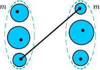
Figure 1: Explosive percolation model rules. At each step, two samples of $m$ vertices are selected at random. In each of the samples, a vertex belonging to the smallest (of $m$) cluster is chosen, and a new edge connecting these two vertices is added to the system.

This model can be treated as an aggregation process, in which clusters selected by our rules merge progressively. A complete description of this process is provided by the evolving distribution $P(s,t)=sn(s)/\langle s\rangle$, which is the probability that a uniformly randomly chosen vertex belongs to a cluster of size $s$ at time $t$. Here $n(s)$ is the size distribution of clusters and $\langle s\rangle$ is the average size of clusters (including the percolation cluster). Let us introduce the probability $Q(s,t)$ that a vertex chosen by our rules from an $m$ vertex sample belongs to a cluster of size $s$. This is the size distribution of merging clusters. Using formulas of probability theory Feller:f68 , we express the distribution $Q(s,t)$ in terms of the distribution $P(s,t)$,

$$Q(s,t)\!=\!\!\left[\sum_{u=s}^{\infty}P(u,t){+}S(t)\!\right]^{m}\!\!\!\!-\left[\!\sum_{\ u=s+1}^{\infty}\!\!\!P(u,t){+}S(t)\!\right]^{m}\!\!\!\!,$$ (1)

which is the basic formula of extreme value statistics. Here $\sum_{u=s}^{\infty}P(u)+S$ is the cumulative distribution. This is the probability that a uniformly randomly chosen vertex belongs to a cluster of size $u\geq s$ including the giant component. Using the normalization condition $\sum_{u=1}^{\infty}P(u)+S=1$, we obtain

$$Q(s,t)=\left[1-\sum_{u=1}^{s-1}P(u,t)\right]^{m}\!\!\!\!-\left[1-\sum_{u=1}^{s}P(u,t)\right]^{m}.$$ (2)

Note also the relation $\sum_{u=1}^{\infty}Q(u)+S^{m}=1$. The evolution equations for the distributions $P(s,t)$ and $Q(s,t)$ describing this aggregation process in the infinite system ($N\to\infty$) have the form

$$\frac{\partial P(s,t)}{\partial t}=s\sum_{u+v=s}Q(u,t)Q(v,t)-2sQ(s,t).$$ (3)

In the case of $m=1$, $Q(s,t)$ in Eq. (3) should be replaced by the distribution $P(s,t)$, and we arrive at well-known master equations for standard percolation, which can be solved explicitly Krapivsky:krb10 . This cannot be done for $m>1$ because in this case the right-hand side of Eq. (3) is not bilinear due to relation (2) and cannot be treated by a generating function technique. Because of this nonlinearity, the case of $m\geq 2$ is far more difficult than that of $m=1$. So we will analyze Eq. (3) numerically, taking into account the relation (2) and a given initial distribution $P(s,0)$. In our work daCosta:ddgm10 we showed that the solution of this equation has a power-law asymptotics

$$P(s,t_{c})\cong f(0)s^{1-\tau}$$ (4)

at the critical point, where the exponent $\tau$ slightly exceeds $2$, which indicates a continuous phase transition. Note that there exist phase transitions combining discontinuity and critical singularity which show a power-law distribution $P(s)\sim s^{-3/2}$ at the critical point Dorogovtsev:dgm06 . In these so-called hybrid transitions, the critical singularity is present when one approaches the critical point only from one side of the transition, namely from the ordered phase. This (the value $\tau=5/2$ and the asymmetry of the hybrid transition) differs sharply from the situation considered in this work. Nonetheless, our method is in principle applicable to hybrid phase transitions as well. The factor $f(0)$ in Eq. (4) is a critical amplitude which equals the value of the scaling function $f(x)$ at $x=0$. At $t\neq t_{c}$, the size distribution of clusters decreases more rapidly than any power law. Near $t_{c}$ we have $P(s,t)=s^{1-\tau}f\left(s|t-t_{c}|^{1/\sigma}\right)$, where $\tau$ and $\sigma$ are critical exponents. While the values of the critical exponents are independent of initial conditions, the form of the scaling function $f(x)$, and so the critical amplitude $f(0)$, depends on the initial distribution $P(s,0)$. Note that initial distributions should decay sufficiently rapidly, faster than a power law with exponent $-2m/(2m-1)$, to produce a nonzero critical point, $t_{c}>0$. The role of initial conditions will be considered elsewhere. Furthermore, the scaling function above the critical point differs from that below $t_{c}$ daCosta:ddgm10 . The dimensionality of our system is infinite, i.e., above the upper critical dimension, which guarantees an exact description in the framework of a mean-field approach. Exact Eqs. (2) and (3) provide this description. As it should be above the upper critical dimension, one can express any critical exponent in this problem in terms of one of them. So we need to find one critical exponent. Similarly to Ref. daCosta:ddgm10 , we find the following relation between the critical exponents $\tau$ and $\beta$ for arbitrary $m$:

$$\beta=\frac{\tau-2}{1-(2m-1)(\tau-2)}$$ (5)

and the expression for the upper critical dimension

$$d_{\text{uc}}=2+4m\beta$$ (6)

above which a mean-field description is exact. The detailed derivation of these relations and the complete scaling theory of the explosive percolation transitions will be presented elsewhere. In Eq. (6) we exploited the fact that the upper critical dimension can be always expressed in terms of the mean-field theory critical exponents. Note that our models, in the present form, are defined in infinite dimensions, and, formally speaking, one cannot directly implement them in lower dimensions. Assume that one can introduce an explosive percolation model of the same universality class of critical behavior (i.e., with the same set of critical exponents) but defined on lattices. Then $d_{\text{uc}}$ is the upper critical dimension of this model. Notice that a bunch of explosive percolation systems on finite-dimensional (mostly two-dimensional) lattices were considered Ziff:z09 .

Let us obtain the critical exponent $\tau$ and the critical amplitude $f(0)$ for $m=2$, $3$, and $4$, as well as the critical point (explosive percolation threshold) $t_{c}$. We assume that at the initial moment all vertices are disconnected, that is $P(s,0)=\delta_{s,1}$, where $\delta_{s,1}$ is the Kronecker symbol. This is our initial condition for the evolution equation.

Substituting Eq. (2) into Eq. (3) we find $P(1,t)$. Substituting this result into the second equation and solving we obtain $P(2,t)$, and so on. This procedure enables us to solve numerically the first $s_{\text{max}}$ equations and find $P(s\leq s_{\text{max}},t)$ at any $t$ with any desired precision.

III The approach

The method we use in this paper is based on the fact that at the critical point, the cluster size distribution $P(s,t_{c})$ has the power-law asymptotics (4), whose parameters, $\tau$ and $f(0)$ we do not know yet. The idea is to glue together the numerical solution $P(s,t)$ and a power-law function at some cluster size $s_{0}\leq s_{\text{max}}$ and then analyze the variation of the result with $s_{0}$. Let us assume first that we know precisely the value of the critical point $t_{c}$, which is actually not the case. Then, after finding numerically $P(s,t_{c})$ for all $s\leq s_{0}$ and gluing it to a power law at $s_{0}$, we easily obtain exponent $\tau$ and critical amplitude $f(0)$. For that, one uses two conditions: (i) $P(s_{0},t_{c})=f(0)s_{0}^{1-\tau}$ and (ii) the normalization condition, namely,

$$\sum_{s=1}^{\infty}P(s,t_{c})=\sum_{s<s_{0}}P(s,t_{c})+f(0)\sum_{s\geq s_{0}}s^{1-\tau}=1.$$ (7)

This condition can be conveniently rewritten in the following form:

$$1=\sum_{s<s_{0}}P(s,t_{c})+P(s_{0},t_{c})s_{0}^{\tau{-}1}\!\!\left[\zeta(\tau{-}1)-\!\sum_{s<s_{0}}\!s^{1-\tau}\!\right]\!,\!\!\!$$ (8)

where $\zeta(x)=\sum_{s=1}^{\infty}s^{-x}$ is the Riemann zeta function. With known $t_{c}$, we would immediately find critical exponent $\tau$ from this equation, leading to the precise value of $\tau$ in the limit $s_{0}\to\infty$.

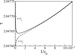
Figure 2: Variation of $\tau$ for $m=2$, calculated from Eq. (10), with $1/s_{0}$, where $s_{0}$ is the point at which numerical solution $P(s,t)$ is glued together with a power law. In our calculations, $s_{0}$ is in the range up to $10^{5}$. The solid and dashed curves correspond to two values of $t$, namely, $t=0.923207<t_{c}$ and $t=0.923208>t_{c}$, respectively.

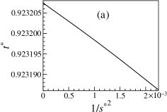
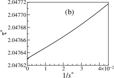
Figure 3: Functions (a) $t(s^{\ast})$ vs. $1/{s^{\ast}}^{2}$, and (b) $\tau(s^{\ast})$ and (c) $f^{*}(0,s^{\ast})$ vs. $1/{s^{\ast}}$ (see the text for the definitions of these functions) in the case of $m=2$. In the limit $s^{*}\to\infty$, the values $t(s^{*})$, $\tau^{*}$, and $f^{\ast}(0)$ approach the exact values of the critical point $t_{c}$, the critical exponent $\tau$, and the amplitude $f(0)$, respectively. These curves are extrapolated to $1/s^{*}{\to}0$ to obtain the precise values $t_{c}$, $\tau$, and $f(0)$.

The value of $t_{c}$ however is not known in advance. Nonetheless, we can formally perform this procedure at any $t$, inserting the numerical solution of the evolution equations for $s\leq s_{0}$ into the following equations:

$$\hskip 38.0ptP(s_{0},t)=f(0)s_{0}^{1-\tau},$$ (9)

$$1=\!\sum_{s<s_{0}}\!P(s,t)+P(s_{0},t)s_{0}^{\tau-1}\!\left[\zeta(\tau{-}1)-\!\sum_{s<s_{0}}\!s^{1-\tau}\right].\!\!\!$$ (10)

From which we can find $\tau$ and $f(0)$ vs. $s_{0}$ for any $t$. Clearly, the exact value of $\tau$ is given by the last equation only for $t=t_{c}$ (when $s_{0}\to\infty$). However, we can still use it to find the set of points $\tau(s_{0})$ corresponding to some time $t\neq t_{c}$. The idea is to analyze how the solutions $\tau(s_{0},t)$ of Eq. (10) vary with $s_{0}$ for a set of $t$ chosen from a neighborhood of the supposed critical point. Below and above the critical point, these solutions behave quite differently as $s_{0}$ approaches infinity, and so it will be easy to identify $t_{c}$. This difference is due to the fact that above $t_{c}$, Eq. (10) neglects the giant component, and the real sum for finite components $\sum_{s=1}^{\infty}P(s,t>t_{c})$ actually equals $1-S<1$.

Figure 2 shows two typical curves $\tau$ vs. $1/s_{0}$ for two particular values of $t$, one below and the other above the critical point (respectively, solid and dashed curves) for the case of $m=2$. With decreasing $1/s_{0}$, these dependencies approach infinity or $2$ if $t$ is below or above $t_{c}$, respectively. One can show that an infinite exponent $\tau(s_{0}\to\infty)$ corresponds to a rapidly decreasing cluster size distribution in the normal phase ($t<t_{c}$). Indeed, apart from the critical point, the distribution $P(s,t)$ decays with $s$ in a exponential-like fashion for large $s$. Numerical solution of the evolution equations gives a distribution of this kind in the range of $s\leq s_{0}$. When we try to glue together this exponential-like function for $s\leq s_{0}$ and a power-law function for $s\geq s_{0}$, we can only get the infinite exponent $\tau$, which corresponds to a more rapid decay than any power law. On the other hand, the behavior $\tau(s_{0})\to 2$, when $s_{0}\to\infty$, indicates the failure of the normalization condition $\sum_{s=1}^{\infty}P(s,t)=1$, which is no longer valid in the phase with a giant component. In this phase, $1-\sum_{s=1}^{s_{0}}P(s,t)$ approaches a nonzero value $S(t)$ as $s_{0}\to\infty$. This violation of normalization to $1$ manifests itself in the divergence of the sum $\sum_{s=s_{0}}^{\infty}s^{1-\tau}$ on its upper limit at $\tau=2$.

If $t=t_{c}$, the curve $\tau(s_{0},t)$ leads to the precise $\tau$ as $1/s_{0}\to 0$. Otherwise, the curves run away from that point, which is the behavior demonstrated by the solid and dashed curves in Fig. 2. To find the precise values of $t_{c}$, $\tau$, and $f(0)$ we inspected a set of $t$. For each of these $t$, we find the minimum of $\tau(s_{0})$, see Fig. 2. Namely, we find the value of this minimum $\tau^{*}=\text{min}_{s_{0}}\tau(s_{0},t)$ and the value $s^{*}$ of $s_{0}$ at which it takes place. We also find the value $f^{\ast}(0)$ corresponding to this minimum, $f^{\ast}(0)=P(s^{*},t){s^{\ast}}^{\tau^{*}-1}$. In particular, these results provide the dependence of the position of the minima $s^{*}$ on $t$. Instead of $s^{*}(t)$, it is convenient to analyze the inverse function $t$ vs. $1/{s^{*}}^{2}$, since we are interested in the limit $s^{*}\to\infty$, and the function $t(1/{s^{*}}^{2})$ is close to linear, see Fig. 3(a). In this limit, $s^{*}\to\infty$, the values $t(s^{*})$, $\tau^{*}$, and $f^{\ast}(0)$ tend to the exact values of the critical point $t_{c}$, the critical exponent $\tau$, and the amplitude $f(0)$, respectively. This figure demonstrates that the curve $t$ vs. $1/{s^{*}}^{2}$ approaches $t_{c}$ almost linearly. Similarly, we plot $\tau^{*}$ and $f^{\ast}(0)$ vs. $1/s^{*}$, see Figs. 3(b) and 3(c), respectively, where each point on the plots corresponds to a different value of $t$. These figures demonstrate that $\tau^{\ast}$ and $f(0)^{\ast}$ approach $\tau$ and, respectively, $f(0)$ almost linearly with $1/s^{\ast}$. This enables us to make extrapolations to $s^{\ast}\to\infty$ (the maximum number of equations which we used, $s_{\text{max}}$, was $10^{5}$) and obtain $t_{c}$, $\tau$, and $f(0)$ with very high precision.

One can even avoid the extrapolation procedure, which may prove to be difficult at $m=4$ and higher. The problem is that for higher $m$ the curves $\tau(s_{0})$ oscillate (see Fig. 4), because the distribution $P(s,t)$ oscillates in the range of low $s$. The reason for these oscillations is the following. If $m$ tends to infinity, then according to our rules, two smallest clusters in the system merge at each step together. Consequently, single vertices initially merge together into the clusters of size $2$, then these clusters merge into the clusters of $4$ vertices, and so on. This results in the peaks of the distribution at $s=2,4,8,\dots$, which are seen already at $m=4$. Fortunately, the amplitude of the oscillations in Fig. 4 decreases with decreasing $1/s_{0}$. This enables us to investigate the run away of the curves from the precise value of $\tau$ at small $1/s_{0}$. As $t$ approaches $t_{c}$ from below or above, the run away in direction of infinity or $2$, respectively, occurs at smaller and smaller values of $1/s_{0}$. It is easy to identify an interval where $t_{c}$ should lie. The lower bound of this interval is the biggest value of $t$ for which the curve $\tau(1/s_{0})$ still shows a trend to infinity at the smallest $1/s_{0}$, i.e., $1/s_{\text{max}}$. The higher bound of the interval is the smallest value of $t$ that corresponds to a curve still demonstrating a trend to $2$ at $1/s_{0}=1/s_{\text{max}}$. Corresponding intervals for $\tau$ and $f(0)$ are then obtained by using Eqs. (9) and (10). We adjust $t$ progressively, using the shooting method, in such a way that the run away takes place at the smallest value of $1/s_{0}$. Even using only the numerical solution of the first $10$ evolution equations this method gives $t_{c}=0.924(2)$ and $\tau=2.047(3)$ for $m=2$. The precision of all the results shown in Table 1 was attained by direct inspection of the curves $\tau(1/s_{0})$, for a $s_{0}\leq s_{\text{max}}=10^{5}$. We tested our method on ordinary percolation ($m=1$) started from isolated nodes. Using $s_{\text{max}}=1000$ recovers the exact values $t_{c}=1/2$ and $\tau=5/2$ with precision $2{\times}10^{-5}$ and $8{\times}10^{-4}$, respectively.

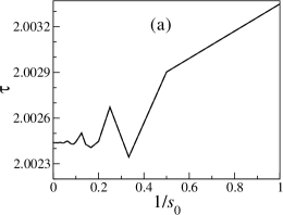
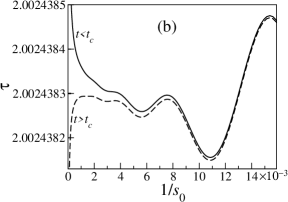
Figure 4: Variation of $\tau$, calculated from Eq. (10), with $1/s_{0}$ in the case of $m=4$. The solid and dashed curves in (a) and (b) correspond to two values of $t$, namely, $t=0.994973560<t_{c}$ and $t=0.994973564>t_{c}$, respectively. Panel (a) shows the full range of $s_{0}$ from $1$ to $s_{\text{max}}=10^{5}$, and panel (b) shows the part of the same plot in the range of $s_{0}$ from $1/16\times 10^{3}$ to $s_{\text{max}}=10^{5}$. In panel (a), the solid and dashed curves are indistinguishable.

Another approach for a model of this class was used in Ref. Vijayaraghavan:vnwd13 to estimate the percolation threshold position imposing the strong assumption that the cluster size distribution $P(s,t)\propto s^{1-\tau}e^{-cs}$, where $c$ is time-dependent, and $c(t_{c})=0$. In this way, after solving $10^{5}$ evolution equations, they achieved the same precision of $t_{c}$ (or even worse) which our method provides with only $10$ equations. One should emphasize that the actual scaling form of the cluster size distribution essentially deviates from a simple exponential, see Ref. daCosta:ddgm10 .

Table 1: Characteristics of the standard percolation ($m=1$) and explosive percolation ($m=2,3,4$) transitions.

$m$	1	2	3	4
$t_{c}$	$1/2$	0.923207509297(2)	0.9817953173509(2)	0.99497356260563(2)
$\beta$	1	0.05557108(1)	0.010428725(1)	0.0024806707(2)
$\tau$	$5/2$	2.04763045(1)	2.009911883(1)	2.0024383299(1)
$d_{\text{uc}}$	$6$	2.4445686(1)	2.12514470(2)	2.039690731(3)
$f(0)$	$1/\sqrt{2\pi}{\approx}0.3989$	0.04619071(1)	0.009831398(1)	0.0024320386(1)
$P(1,t_{c})$	$1/e{\approx}0.3678$	0.0485928295546(4)	0.01172146480245(2)	0.003343067143133(1)

IV Critical exponents and amplitudes

The results of the application of this numerical method to the models with $m=2$, $3$, and $4$ are presented in Table 1. For comparison, in the first column of the table, we show the exact values for the ordinary percolation problem ($m=1$). The values of the exponent $\beta$ and the upper critical dimension $d_{\text{uc}}$ are found by using relations (5) and (6). In the case of $m=2$, the values presented in the table agree with our results daCosta:ddgm10 , although the precision of the numbers obtained in the present work is much higher despite the fact that here we solved $10$ times fewer evolution equations than in Ref. daCosta:ddgm10 . Furthermore, the results in the table for the models with $2\leq m\leq 4$ agree with those obtained from equations for scaling functions (we will consider this alternative method elsewhere). As $m$ increases, the difference $1-t_{c}$ decreases, and the exponent $\beta$ of the giant component size also decreases. The critical amplitude $f(0)$ is close to $P(1,t_{c})$, especially when $m\leq 3$. This closeness indicates that the deviations from a power-law asymptotics in these problems are small even at low values of $s$. Note that $f(0)>P(1,t_{c})$ for classical percolation, while the opposite is true for the explosive percolation transition. The values of $\beta$ are remarkably small. In particular, in the case of $m=4$, $\beta$ is close to $1/400$. This produces an extremely “sharp” transition whose continuity is virtually unobservable even in astronomically large though finite systems. One should note that our way to vary exponents in these non-universal systems by changing $m$ is not unique. For example, other explosive percolation models, introduced in Refs. Fan:fllc12 ; Andrade:ah13 , showed a decay of $\beta$, controlled by a different, specially introduced model parameter.

V Discussions and conclusions

Our results show a rapid decrease of the critical exponent $\beta$ values with increasing $m$. For $m=4$, exponent $\beta$ is about 20 times smaller than already its tiny value for $m=2$. This indicates that exploration of this transition by means of numerical simulations at higher $m$ is hardly possible. Table 1 demonstrates that the upper critical dimension $d_{\text{uc}}$ quickly approaches $2$ with increasing $m$. So the explosive percolation transition in models of this class placed on two-dimensional lattices is very close to its upper critical dimension. This suggests that the critical characteristics of explosive percolation on two-dimensional systems should be close to what was obtained in this paper.

We emphasize that our results were found for models in which evolution is determined by purely local optimization rules. It means that each new interconnection uses only a finite amount of information. In particular, to establish a new link, we do not need to know which of clusters is the biggest in the system. (Indeed, to find the largest cluster, one has to know about all of them.) It is the local optimization rule that leads to continuity of the explosive percolation transition in these models. In more exotic models employing various global optimization algorithms and their variations, discontinuities may occur Schrenk:sah11 ; Chen:cczcdn13 ; Riordan:rw12 ; Chen:cncjszd13 ; Schrenk:sfdadh12 ; Araujo:ah10a ; Cho:chhk13 .

In summary, we have proposed an effective numerical method enabling us to find characteristics of explosive percolation transitions with high precision. We obtained the critical points, critical exponents, and critical amplitudes in a set of representative models. The fact that critical exponents are model dependent demonstrates the non-universality of critical phenomena for this phase transition. Our results confirm the conclusion that explosive percolation transitions are continuous, with a power-law form of the cluster size distribution at the critical point. Based on our observations, we suggest that in a wide range of models of this kind the explosive percolation transition is continuous, including in particular, the models considered in Refs. Achlioptas:ads09 ; Nagler:nlt11 ; Ziff:z09 ; Radicchi:rf09 ; Cho:ckp09 ; Cho:ckk10 ; D'Souza:dm10 ; Manna:mc11 ; Friedman:fl09 ; Choi:cyk11 .

Our approach provides a useful tool for a quantitative description of a new class of critical phenomena in non-equilibrium systems and irreversible processes. Moreover, the applicability of this numerical method is not limited to explosive percolation models. Since the method relies only on generic scaling properties, it is suitable to a wide range of continuous phase transitions in non-equilibrium systems.

- (1) D. Stauffer and A. Aharony, Introduction to Percolation Theory (Taylor & Francis, London, 1994).
- (2) D. Stauffer, Phys. Rep. 54, 1 (1979).
- (3) S. N. Dorogovtsev, A. V. Goltsev, and J. F. F. Mendes, Rev. Mod. Phys. 80, 1275 (2008).
- (4) S. N. Dorogovtsev and J. F. F. Mendes, Evolution of Networks: From Biological Nets to the Internet and WWW (Oxford University Press, New York, 2003).
- (5) S. N. Dorogovtsev and J. F. F. Mendes, Adv. Phys. 51, 1079 (2002).
- (6) S. N. Dorogovtsev, Lectures on Complex Networks (Oxford University Press, Oxford, 2010).
- (7) D. Achlioptas, R. M. D’Souza, and J. Spencer, Science 323, 1453 (2009).
- (8) Y. S. Cho, J. S. Kim, J. Park, B. Kahng, and D. Kim, Phys. Rev. Lett. 103, 135702 (2009).
- (9) F. Radicchi and S. Fortunato, Phys. Rev. Lett. 103, 168701 (2009).
- (10) R. M. Ziff, Phys. Rev. Lett. 103, 045701 (2009).
- (11) Y. S. Cho, B. Kahng, and D. Kim, Phys. Rev. E 81, 030103 (R) (2010).
- (12) R. M. Ziff, Phys. Rev. E 82, 051105 (2010).
- (13) N. A. M. Araújo, J. S. Andrade Jr., R. M. Ziff, and H. J. Herrmann, Phys. Rev. Lett. 106, 095703 (2011).
- (14) R. A. da Costa, S. N. Dorogovtsev, A. V. Goltsev, and J. F. F. Mendes, Phys. Rev. Lett. 105, 255701 (2010).
- (15) O. Riordan and L. Warnke, Science 333, 322 (2011).
- (16) J. Nagler, A. Levina, and M. Timme, Nature Phys. 7, 265 (2011).
- (17) P. Grassberger, C. Christensen, G. Bizhani, S.-W. Son, and M. Paczuski, Phys. Rev. Lett. 106, 225701 (2011).
- (18) H. K. Lee, B. J. Kim, and H. Park, Phys. Rev. E 84, 020101(R) (2011).
- (19) J. H. Qian, D. D. Han, and Y. G. Ma, Europhys. Lett., 100, 48006 (2012).
- (20) M. v. Smoluchowski, Ann. Phys. 353, 1103 (1916).
- (21) F. Leyvraz and H. R. Tschudi, J. Phys. A: Math. Gen. 14, 3389 (1981).
- (22) W. Feller, An Introduction to Probability Theory and Its Applications (John Wiley & Sons, New York, 1968), Vol. 1.
- (23) P. L. Krapivsky, S. Redner, and E. Ben-Naim, A Kinetic View of Statistical Physics (Cambridge University Press, Cambridge, 2010).
- (24) S. N. Dorogovtsev, A. V. Goltsev, and J. F. F. Mendes, Phys. Rev. Lett. 96, 040601 (2006).
- (25) V. S. Vijayaraghavan, P.-A. Noël, A. Waagen, and R. M. D’Souza, Phys. Rev. E 88, 032141 (2013).
- (26) J. Fan, M. Liu, L. Li, and X. Chen, Phys. Rev. E 85, 061110 (2012).
- (27) R. F. S. Andrade and H. J. Herrmann, Phys. Rev. E 88, 042122 (2013).
- (28) K. J. Schrenk, N. A. M. Araújo, and H. J. Herrmann, Phys. Rev. E 84, 041136 (2011).
- (29) Y. S. Cho, S. Hwang, H. J. Herrmann, and B. Kahng, Science 339, 1185 (2013).
- (30) N. A. M. Araújo and H. J. Herrmann, Phys. Rev. Lett. 105, 035701 (2010).
- (31) W. Chen, X. Cheng, Z. Zheng, N. N. Chung, R. M. D’Souza, and J. Nagler, Phys. Rev. E 88, 042152 (2013).
- (32) W. Chen, J. Nagler, X. Cheng, X. Jin, H. Shen, Z. Zheng, and R. M. D’Souza, Phys. Rev. E 87, 052130 (2013).
- (33) K. J. Schrenk, A. Felder, S. Deflorin, N. A. M. Araújo, R. M. D’Souza, and H. J. Herrmann, Phys. Rev. E 85, 031103 (2012).
- (34) O. Riordan and L. Warnke, Phys. Rev. E 86, 011129 (2012).
- (35) R. M. D’Souza and M. Mitzenmacher, Phys. Rev. Lett. 104, 195702 (2010).
- (36) S. S. Manna and A. Chatterjee, Physica A 390, 177 (2011).
- (37) E. J. Friedman and A. S. Landsberg, Phys. Rev. Lett. 103, 255701 (2009).
- (38) W. Choi, S.-H. Yook, and Y. Kim, Phys. Rev. E 84, 020102 (2011).