Sustained RF oscillations from thermally induced spin-transfer torque

Abstract

We investigate the angular dependence of the spin torque generated when applying a temperature difference across a spin-valve. Our study shows the presence of a non-trivial fixed point in this angular dependence, i.e. the possibility for a temperature gradient to stabilize radio frequency oscillations without the need for an external magnetic field. This so called ”wavy” behavior can already be found upon applying a voltage difference across a spin-valve but we find that this effect is much more pronounced with a temperature difference. Our semi-classical theory is parametrized with experimentally measured parameters and allows one to predict the amplitude of the torque with good precision. Although thermal spin torque is by nature less effective than its voltage counterpart, we find that in certain geometries, temperature differences as low as a few degrees should be sufficient to trigger the switching of the magnetization.

Spin caloritronicsBauer et al. (2012); Hatami et al. (2007); Jia et al. (2011); Uchida et al. (2008, 2010); Kikkawa et al. (2013); Jia and Berakdar (2013) studies the interplay of charge, spin and heat transport and provides extensions to some of the spintronics concepts. One of interest to us is the spin-transfer torque (STT)Ralph and Stiles (2008); Myers et al. (1999); Katine et al. (2000), first predicted by Slonczewski and Berger in 1996Slonczewski (1996); Berger (1996). STT is the angular momentum deposited by a spin-polarized current on a ferromagnetic layer. It is at the origin of interesting out of equilibrium dynamics for the magnetization layer leading to magnetic reversal or sustained RF oscillations. The later effect, known as spin-torque oscillator (STO)Li and Zhang (2003); Houssameddine et al. (2009) is a promising candidate for agile RF sources. Although most STO require an external magnetic field, it was also discovered that STT can, in some very asymmetric spin-valves, stabilize an oscillating state in the absence of an external magnetic field. This is the so-called wavinessBoulle et al. (2008); Rychkov et al. (2009); Gmitra and Barnaś (2009). In 2007, in one of the first article on ”caloritronics”, Bauer et al. considered another route for creating STT via the combination of spintronics with thermoelectric effectsHatami et al. (2007): the so-called thermal STT. Spin-dependent thermoelectric effects soon started to attract some theoretical and experimental interest Slonczewski (2010); Uchida et al. (2008, 2010); Kikkawa et al. (2013); Dejene et al. (2012); Flipse et al. (2012)

In this letter, we investigate the angular dependence of the STT induced by temperature gradients applied across various type of magnetic spin valves. Our semi-classical theory, carefully tabulated with experimentally measured parameters, shows that thermally-induced STT is naturally ”wavy” for a wide range of devices. By optimizing the geometry of the sample, we predict that magnetic switching can be obtained with temperature differences as low as a few degrees.

Semi-classical drift-diffusion approach. Our starting point is a semi-classical approached for metallic magnetic multilayers that treats the charge degrees of freedom at the drift-diffusion level yet retains all the information about spin degrees of freedomWaintal et al. (2000); Rychkov et al. (2009). This approach to which we refer as CRMTWaintal et al. (2000); Rychkov et al. (2009); Borlenghi et al. (2011) (for Continuous Random Matrix Theory) can be seen as a generalization of the Valet Fert theoryValet and Fert (1993) to systems with non collinear magnetizationPetitjean et al. (2012). It is also equivalent to the so-called (Generalized) Circuit TheoryBauer et al. (2003). Here we generalize CRMT to include heat flow and thermoelectric effects. In addition to the charge $I_{\alpha}$ and spin $\boldsymbol{J}_{\alpha}$ current densities, we therefore add the heat current density $Q_{\alpha}$ ($\alpha=x,y,z$ being the direction of propagation). Similarly, in addition to the charge $\mu_{c}$ and spin $\boldsymbol{\mu}$ potentials, we include the temperature $\theta$ (in energy unit, $\theta=k_{B}T$ where $T$ is the actual temperature). Note that in this letter, we assume that a single temperature can be defined for both majority and minority electrons. Thermoelectric effects are described by spin dependent Seebeck and Peltier coefficientsBakker et al. (2010); Slachter et al. (2011); Dejene et al. (2012); Uchida et al. (2008). We note $S_{\uparrow}$ ($S_{\downarrow}$) the spin-dependent Seebeck coefficients for majority (minority) electrons while the Peltier coefficients are given by Onsager relation $\Pi_{\sigma}=S_{\sigma}T^{*}$ where $T^{*}$ is the average temperature. We further introduce dimensionless Seebeck coefficients in unit of $k_{B}/e\approx 80\mu V.K^{-1}$: $s=e(S_{\uparrow}+S_{\downarrow})S/(2k_{B})$ and $\Delta s=e(S_{\uparrow}-S_{\downarrow})S/(2k_{B})$ characterize respectively the average and the polarization of the Seebeck effect. Recent experiments provide the first spin resolved values of these quantities for ferromagnetic materialsDejene et al. (2012): $s_{Co}\approx-0.25$ and $\Delta s_{Co}\approx-0.02$ for cobalt, and $s_{Py}\approx-0.21$ and $\Delta s_{Py}\approx-0.044$ for permalloy. We introduce reduced currents (with unit of energy) as follows,

$$I_{\alpha} =4j_{\alpha}^{c}/(e{\cal R_{\rm Sh}})$$ (1)

$$\boldsymbol{J}_{\alpha} =2\hbar\boldsymbol{j}_{\alpha}/(e^{2}{\cal R_{\rm Sh}})$$ (2)

$$Q_{\alpha} =4k_{B}T^{*}j_{\alpha}^{q}/(e^{2}{\cal R_{\rm Sh}})$$ (3)

where ${\cal R_{\rm Sh}}$ is the Sharvin resistance for a unit surface ( with typical value ${\cal R_{\rm Sh}}\approx 1f\Omega.m^{2}$), and $e<0$ is the charge of the electron. These variables follow a set of Ohm-like (or Fourier-like) equations,

$$-\ell_{\ast}\partial_{\alpha}\mu_{c} =j_{\alpha}^{c}-\beta\boldsymbol{j}_{\alpha}\cdot\boldsymbol{m}+\dfrac{\ell_{\ast}}{\ell_{H}}s\left(sj_{\alpha}^{c}+\Delta s\boldsymbol{j}_{\alpha}\cdot\boldsymbol{m}\right)-\dfrac{\ell_{\ast}}{\ell_{H}}sj_{\alpha}^{q}$$ (4)

$$-\ell_{\ast}\partial_{\alpha}\boldsymbol{\mu} =\boldsymbol{j}_{\alpha}-\beta j_{\alpha}^{c}\boldsymbol{m}+\dfrac{\ell_{\ast}}{\ell_{H}}\Delta s\left(sj_{\alpha}^{c}\boldsymbol{m}+\Delta s\boldsymbol{j}_{\alpha}\right)-\dfrac{\ell_{\ast}}{\ell_{H}}\Delta sj_{\alpha}^{q}\boldsymbol{m}+\dfrac{\ell_{\ast}}{\ell_{\perp}}\left(\boldsymbol{m}\times\boldsymbol{j}_{\alpha}\right)\times\boldsymbol{m}-\dfrac{\ell_{\ast}}{\ell_{L}}\left(\boldsymbol{m}\times\boldsymbol{j}_{\alpha}\right)$$ (5)

$$-\ell_{H}\partial_{\alpha}\theta =-sj_{\alpha}^{c}-\Delta s\boldsymbol{j}_{\alpha}\cdot\boldsymbol{m}+j_{\alpha}^{q}$$ (6)

Eqs(4-6) are the extension of Eqs.(1)-(4) of Petitjean et al. (2012). The unit vector $\boldsymbol{m}$ is the local direction of the magnetization (bold vectors correspond to spin space while explicit components $\alpha=x,y,z$ are used for real space). The parameters involved are the mean free paths for the majority ($\ell_{\uparrow}$) and minority ($\ell_{\downarrow}$) electrons, related to the spin-dependent resistivities $\rho_{\sigma}$ as $\ell_{\uparrow(\downarrow)}={\cal R_{\rm Sh}}/\rho_{\uparrow(\downarrow)}$. They can be expressed alternatively in term of $\ell_{\ast}$, the average mean free path ($1/\ell_{\ast}=1/\ell_{\uparrow}+1/\ell_{\downarrow}$), and $\beta=(\ell_{\uparrow}-\ell_{\downarrow})/(\ell_{\uparrow}+\ell_{\downarrow})$, the asymmetry of the spin resolve asymmetry (with a definition identical to the usual Valet-Fert parameter). Two length scales characterize the behavior of a spin perpendicular to the magnetization: the Larmor precession length $\ell_{L}$ and the transverse penetration length $\ell_{\perp}$, see Petitjean et al. (2012). Finally, $\ell_{H}$ is the heat diffusion length. For purely electronic heat transfer Wiedemann-Franz law implies, $\ell_{H}=\ell_{\ast}(\mathcal{L}-s^{2}+2\beta s\Delta s+\Delta s^{2})/(1-\beta^{2})$ with $\mathcal{L}=\pi^{2}/3$. However, to account for the phonon contribution, higher values of $\mathcal{L}$ can be used. A second set of equation expresses the conservation (or lack thereof) of the different currents,

$$\sum_{\alpha}\partial_{\alpha}j_{\alpha}^{c} =0$$ (7)

$$\sum_{\alpha}\partial_{\alpha}j_{\alpha}^{q} =0$$ (8)

$$\sum_{\alpha}\partial_{\alpha}\boldsymbol{j}_{\alpha} =-\dfrac{\ell_{\ast}}{\ell_{sf}^{2}}\boldsymbol{\mu}-\dfrac{1}{\ell_{\perp}}\left(\boldsymbol{m}\times\boldsymbol{\mu}\right)\times\boldsymbol{m}+\dfrac{1}{\ell_{L}}\left(\boldsymbol{m}\times\boldsymbol{\mu}\right)$$ (9)

where $\ell_{sf}$ is the spin diffusion length. Similarly, a set of equations describe the interface boundary conditions between a ferromagnet and a normal metal. The charge and spin sectors are described by the usual spin dependent interface resistances $r^{b}_{\sigma}$, namely Equation (8) and (9) of Ref.Petitjean et al. (2012). The heat sector is given by (neglecting interface thermoelectric effects),

$$\sum_{\alpha}n_{\alpha}j_{\alpha}^{q} =\mathcal{L}\dfrac{{\cal R_{\rm Sh}}}{4r^{b}_{\ast}(1-\gamma^{2})}(\theta_{N}-\theta_{F})$$ (10)

Where $\theta_{N}$ and $\theta_{F}$ are the temperatures on both sides of the Ferro-Normal interface and the interface resistances have been parametrized according to the usual Valet-Fert notation $r^{b}_{\uparrow,\downarrow}=2r^{b}_{\ast}(1\pm\gamma)$. $n_{\alpha}$ are the components of the normal unit vector pointing towards the magnetic side of the interface. Last, the boundary conditions at the metallic electrodes are given by Eqs.(12) and (13) of Ref.Petitjean et al. (2012) for the spin and charge sector while the heat sector reads ($n_{\alpha}$ points towards the system),

$$\sum_{\alpha}n_{\alpha}j_{\alpha}^{q}+\theta=k_{B}\Delta T$$ (11)

where $k_{B}\Delta T$ is the temperature difference applied to the reservoir with respect to the reference temperature $T^{*}$.

Application to thermally induced STT in a spin-valve Let us now turn to a spin-valve made of the following stack: $\rm{Cu_{20}|Co_{L_{Co}}|Cu_{2}|Py_{L_{Py}}(\varphi)|Cu_{10}}$ where the indices indicate the corresponding thicknesses in nm and $\varphi$ is the angle of the magnetization of the free (permalloy) layer with respect to the fixed cobalt layer. Following usual practiceSlonczewski (1996); Waintal et al. (2000), the torque $\boldsymbol{\tau}$ exerted on the free layer is defined as the difference of spin currents on both side of the layer (spin relaxation only provides extremely small corrections here, seePetitjean et al. (2012)). We used standard material parameters for the mean free paths and spin-diffusion lengths of Cu, Co and Py, as extracted from giant magneto resistance measurementsPetitjean et al. (2012)) while we focus on the values given in RefDejene et al. (2012) for the spin resolved Seebeck coefficients (see supplementary material).

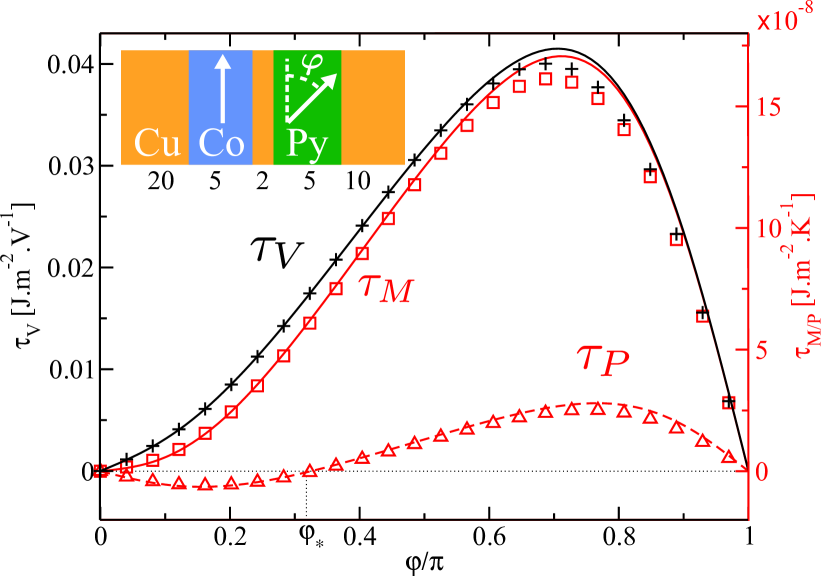
Figure 1: Spin-transfer torque obtained when applying a voltage ($\tau_{V}$, bottom curve), a temperature gradient ($\tau_{M}$, top full curve), and a temperature gradient in the open-circuit configuration ($\tau_{P}$, top dashed curve), versus the magnetization angle $\varphi$ of the Py layer with respect to that of the Co layer. Symbols represent the simulations including spin-flip scattering, while lines correspond to the analytical calculation eq:torque. Here $L_{Co}=L_{Py}=5$ nm. Inset: sketch of the spin valve.

fig:torques shows the angular dependence of the spin torque for three different types of setups (see the right part of Fig.2 for a cartoon). In the first, we apply a voltage bias $V_{b}$ across the spin valve and calculate the torkance $\tau_{V}=d\tau/dV_{b}$. We recover the usual feature of STT in metallic spin valve with a stronger torque in the anti-parallel configuration than in the parallel one (black curves). In the second, we apply a temperature difference $\Delta T$ across the spin valve in an open circuit configuration so that no current can flow through the device. This is the ”pure” spin Seebeck case $\tau_{P}=d\tau/d\Delta T$ as it is given by spin current only. In the last closed circuit or ”mixed” configuration, a temperature difference is applied and a current can flow through the spin valve (i.e. the two electrodes of the spin valve are electrically - but not thermally - short circuited). In this last configuration the Seebeck effect induces a finite current density which in turn induces a STT very similar to the voltage driven one. Hence, one find that the mixed thermal torkance $\tau_{M}=d\tau/d\Delta T$ is somehow intermediate between the pure and the voltage torkances. The most remarkable feature of fig:torques is the appearance in the pure case $\tau_{P}$ of a finite angle $\varphi^{*}\approx\pi/3$ where $\tau_{P}$ vanishes. Depending on the sign of the thermal gradient, this new fixed point will be stabilized or destabilized. When stabilized, it corresponds to a fast precessional state which forms a STO. In the context of voltage induced torque, these ”wavy” structures, which do not require magnetic field in contrast to more conventional STOs, have been discussed for highly asymmetric spin valvesBoulle et al. (2008); Rychkov et al. (2009); Gmitra and Barnaś (2009). Here we find that thermally induce STT corresponds to a wavy angular dependence of the torque in a much broader range of parameters. fig:phase diagram, shows the ”phase diagram” of the spin valve as a function of the thicknesses $L_{Co}$ and $L_{Py}$ of the fixed cobalt and free permalloy layers. The various regions correspond to the presence of a wavy angular dependence of the torque for thermal induced spin torque (P and M) and the standard voltage induced STT (V). The color measures the waviness angle of $\tau_{P}$, when it exists.

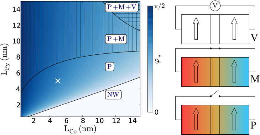
Figure 2: Left: Waviness angle $\varphi^{*}$ of the pure thermal torque $\tau_{P}$ as a function of $L_{Co}$ and $L_{Py}$. The white cross indicates value $L_{Co}=L_{Py}=5$ nm corresponding to fig:torques. The presence of a letter V, M or P in a given region means that the angular dependence of the corresponding torkance $\tau_{V}$, $\tau_{M}$ or $\tau_{P}$ is wavy. NW indicates the region where none of them are wavy. Right: cartoon of our three measurement setups V, M, and P. In M and P a temperature difference is applied across the pillar.

This diagram illustrates several points, the first of which is that thermally induced torque is wavy in a much broader range of thicknesses than the voltage induced torque. Second, the various torques behave quite differently. A thicker Co layer is beneficial for the waviness of $\tau_{V}$, whereas it is detrimental for that of $\tau_{P}$ and $\tau_{M}$. Also, for the limit of a very thin Co layer, the waviness angle for $\tau_{P}$ comes close to $\pi/2$. As a comparison, the maximum waviness angle in this diagram for $\tau_{V}$ (not represented) is five times lower.

To proceed, we introduce a minimum model to estimate the critical value of the temperature gradient needed to trigger magnetic switching or STO behavior. In the macrospin approximation in presence of a purely uniaxial anisotropy, the critical torque (per unit angle and per unit surface of the spin valve) needed to destabilize the initial (parallel or anti-parallel) configuration is given by Slonczewski (1996); Parcollet and Waintal (2006), $\partial\tau/\partial\varphi=\alpha M_{s}L_{Py}B_{u}$ where $B_{u}$ is the uniaxial anisotropy field, $\alpha$ the Gilbert damping coefficient and $M_{s}$ the magnetization. Using $\tau=\tau_{P}\Delta T$, we obtain the critical value of the temperature gradient $\Delta T_{P}$ needed to get magnetic switching (or STO) as,

$$\Delta T_{P}=\frac{\alpha M_{s}B_{u}L_{Py}}{\partial\tau_{P}/\partial\varphi}\approx\frac{L_{Py}}{\partial\tau_{P}/\partial\varphi}\times 1.67\mathrm{\ kJ\cdot m^{-3}\cdot rad^{-1}}$$ (12)

The numerical value of the right hand side of the previous expression was obtained by simulating the spin-valve $\rm{Py_{24}|Cu_{10}|Py_{6}(\varphi)}$ of AlHajDarwish et al. (2004) for which a critical switching current $\rm{I_{crit}=10^{7}A\cdot cm^{-2}}$ has been reported. We calculate a corresponding critical torque of the order of $10^{-5}\rm{J\cdot m^{-2}\cdot rad^{-1}}$ which allows us to estimate globally the product $\alpha M_{s}B_{u}$. Critical currents of the order of $10^{7}\rm{A\cdot cm^{-2}}$ are rather standard values for current driven STTJiang et al. (2004); Zhang et al. (2002); AlHajDarwish et al. (2004) and values up to two orders of magnitude smaller have been reportedYang et al. (2008), so that the previous expression is a rather conservative estimate.

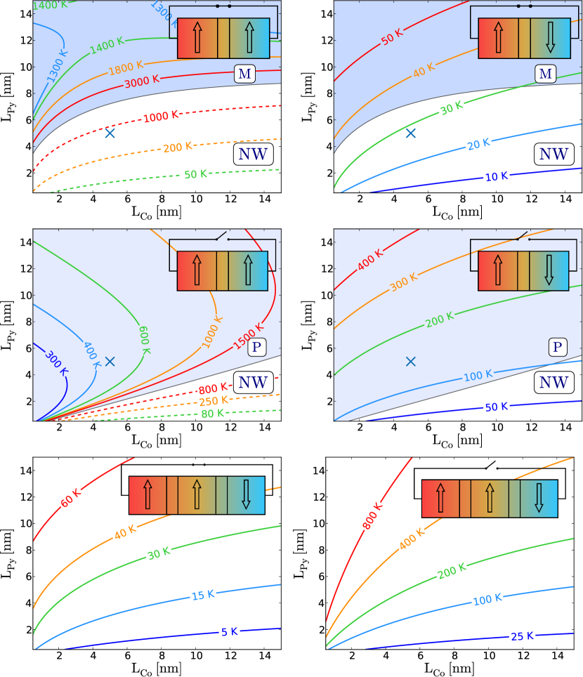
Figure 3: Temperature difference $\Delta T$ needed to achieve the critical torque as a function of $L_{Co}$ and $L_{Py}$ for the mixed ($\Delta T_{M}$, top row) and pure ($\Delta T_{P}$, middle row) torques, for a parallel (left column) and antiparallel (right column) configuration, in the $\rm{Cu_{40}|Co_{L_{Co}}|Cu_{2}|Py_{L_{Py}}(\varphi)|Cu_{10}}$ stack. Dashed ligns indicate a negative torkance. The blue cross indicates $L_{Co}=L_{Py}=5$ nm, cf fig:torques. The background displays the waviness domains of fig:phase diagram. The bottom row shows the same critical temperature difference for the stack $\rm{Cu_{40}|Co_{L_{Co}}|Cu_{2}|Py_{L_{Py}}(\varphi)|Cu_{2}}|Co_{L_{Co}}|Cu_{40}$ for the mixed (left) and pure (right) torques.

fig:critical temperature shows the critical temperature difference in the mixed ($\Delta T_{M}$, top row) and pure case $\Delta T_{P}$, middle row). The corresponding values for the parallel configuration (left column) are very high and are not reasonable for actual devices using the reported values for the Seebeck coefficients (although one should bear in mind that careful tuning of the material/geometrical properties could be use to decrease these values significantly). However, the temperature gradient needed to destabilize the anti-parallel configuration (right panel) is much smaller and should be within experimental grasp (a few tens of Kelvin). To further decrease the critical temperature, we consider a slightly different stack (bottom row of fig:critical temperature) where a third magnetic layer, antiparallel to the first (polarizing) layer has been introduce to enhance the torque. Such an extra layer makes the system perfectly symmetric and therefore makes the waviness behavior disappear. On the other hand, we find a very significant lowering of the critical temperature down to values of a few Kelvin. We find such a low threshold for magnetic reversal to be very encouraging.

Analytical approach: building efficient effective materials. In the absence of spin-flip scattering, ignoring the finite penetration of transverse spins and keeping only the first order terms from the Seebeck/Peltier effect, close analytical expressions can be obtain for our model. A first result is that many collinear materials (or interfaces) put in series can be combined to obtain a unique effective material. After such a procedure our spin valve can be reduced to two effective layers A and B whose magnetizations make an angle $\varphi$. The effective parameters read,

$$\overline{r}=\displaystyle\sum_{i}r_{i}$$ (13)

$$\overline{r}\overline{\beta}=\sum_{i}r_{i}\beta_{i}$$ (14)

$$\overline{r}(1-\overline{\beta}^{2})/{\overline{\mathcal{L}}}=\displaystyle\sum_{i}r_{i}(1-\beta_{i}^{2})/{\mathcal{L}_{i}}$$ (15)

$${\overline{r}}\left(1-\overline{\beta}^{2}\right){\overline{s}}/{\overline{\mathcal{L}}}=\displaystyle\sum_{i}r_{i}(1-\beta_{i}^{2}){s_{i}}/{\mathcal{L}_{i}}$$ (16)

$${\overline{r}}\left(1-\overline{\beta}^{2}\right){\overline{\Delta s}}/{\overline{\mathcal{L}}}=\displaystyle\sum_{i}r_{i}(1-\beta_{i}^{2}){\Delta s_{i}}/{\mathcal{L}_{i}}$$ (17)

where the resistance $r_{i}$ of a bulk layer (interface) is given by the ratio $2\rho_{\ast}L_{i}/{\cal R_{\rm Sh}}$, where $L_{i}$ is the thickness of the layer ($2r_{b}^{\ast}/{\cal R_{\rm Sh}}$). These equations can form the basis for engineering the effective parameters and increase the torkance of the stack. By placing two of these effective materials A and B in series, we obtain a general description of a spin-valve $F_{A}|N|F_{B}(\varphi)$. After some algebra, we obtain the expression of the torque on layer B,

$$\tau=-\dfrac{F}{2}\sin\varphi\left\{\left[\beta_{A}\dfrac{r_{B}+1}{r_{B}}-\beta_{B}\cos\varphi\right]\left(GYeV_{b}+Sk_{B}\Delta T\right)\right.$$

$$+\left.\left[\dfrac{\Delta s_{A}}{\mathcal{L}_{A}}(1-\beta_{A}^{2})\dfrac{r_{B}+1}{r_{B}}-\dfrac{\Delta s_{B}}{\mathcal{L}_{B}}(1-\beta_{B}^{2})\cos\varphi\right]Kk_{B}\Delta T\right\}$$ (18)

where $F$, $G$, $Y$, $K$ and $S$ are expressions involving the various material parameters whose sign do not change when $\varphi$ varies (see supplementary material for explicit expressions). We have checked eq:torque against our numerical simulations and found excellent agreement (see fig:torques). We find that the current $j^{c}\propto GYeV_{b}+Sk_{B}\Delta T$ so that the open-circuit condition for $\tau_{P}$ is obtained using $GYeV_{b}+Sk_{B}\Delta T=0$. While the expression of eq:torque is somewhat cumbersome, the analysis of its angular dependence allows one to obtain simple criteria for the existence of a wavy regime. We find,

$$\cos\varphi_{\ast}^{V} =\dfrac{\beta_{A}}{\beta_{B}}\dfrac{r_{B}+1}{r_{B}}$$ (19)

$$\cos\varphi_{\ast}^{P} =\dfrac{1-\beta_{A}^{2}}{1-\beta_{B}^{2}}\dfrac{\mathcal{L}_{B}}{\mathcal{L}_{A}}\dfrac{\Delta s_{A}}{\Delta s_{B}}\dfrac{r_{B}+1}{r_{B}}$$ (20)

where the above expressions provide first a criterion for waviness ($|\cos\varphi_{\ast}|\leq 1$) and second the value of $\varphi_{\ast}$ for wavy structures. We find that the criterion for waviness in the ”pure” thermal case contains two conflicting contributions: in order to obtain a wavy structure one needs the polarization of the resistivity of the free (B) layer to be small while the corresponding Seebeck coefficient is highly spin polarized. As both are not necessarily correlated (the former is related to the polarization of the density of state while the latter to its variation with respect to energy), this leaves much room for material optimization.

Conclusion. We have developed a quantitative theory for spin dependent Seebeck and Peltier effects in magnetic metallic devices. The theory relies entirely on measured material parameters so that its results do not depend on a - always precarious - detailed microscopic modeling. We find that temperature gradient as low as a few degrees should be enough for magnetic switching. Such low temperature gradients could be used in spintronics devices, either alone or to assist current induced switching.

Acknowledgement Funding was provided by the FP7 project STREP MACALO and the consolidator ERC grant MesoQMC.

I Derivation of the spin torque expression Frefeq:torque

eq:torque was derived in the case of a spin-valve $F_{A}|N|F_{B}(\varphi)$, under the following assumptions: (i) the spin-valve has no variations along the $y$ and $z$ directions, (ii) spin-flip scattering is neglected, (iii) the transverse spin is absorbed at the Normal-Ferro interface ($\ell_{\perp}$ very short) , (iv) the Seebeck coefficients $s$ and $\Delta s$ are only considered at first order and (v) the various layers that make the two effective materials $F_{A}$ and $F_{B}$ have a single orientation of their magnetization. The normal spacer is taken to be perfectly transparent without loss of generality as any finite resistance can be incorporated in the effective material $F_{A}$ or $F_{B}$. We note that in the numerics presented in the main text, condition (ii) and (iv) are relaxed which only lead to small corrections to the results.

Within this set of approximations, eq:crmt1 to (9) become for each material:

$$-\ell_{\ast}\frac{d\mu_{c}}{dx} =j^{c}-\beta j_{\parallel}-s^{\prime}j^{q}$$ (SM-21)

$$-\ell_{\ast}\frac{d\mu_{\parallel}}{dx} =j_{\parallel}-\beta j^{c}-\Delta s^{\prime}j^{q}$$ (SM-22)

$$-\ell_{\ast}\frac{d\theta}{dx} =-s^{\prime}j^{c}-\Delta s^{\prime}j_{\parallel}+\frac{(1-\beta^{2})}{\mathcal{L}}j^{q}$$ (SM-23)

and the conservation equations are:

$$\frac{dj^{c}}{dx} =0$$ (SM-24)

$$\frac{dj^{q}}{dx} =0$$ (SM-25)

$$\frac{dj_{\parallel}}{dx} =0$$ (SM-26)

with $j_{\parallel}=\boldsymbol{j}\cdot\boldsymbol{m}$, $\mu_{\parallel}=\boldsymbol{\mu}\cdot\boldsymbol{m}$, $s^{\prime}=\dfrac{1-\beta^{2}}{\mathcal{L}}s$ and $\Delta s^{\prime}=\dfrac{1-\beta^{2}}{\mathcal{L}}\Delta s$

The conservation equations imply that $j^{c}$ and $j^{q}$ are constant, and the absence of spin-flip makes $j_{\parallel}$ piecewise constant. As a consequence, $\mu_{c}$, $\theta$ and $\mu_{\parallel}$ are piecewise linear so that eq:bulk1 to eq:bulk3 can be easily integrated leading to the effective materials described in Eqs.(13) - (17). The matching of spin accumulation of the $a$ ferromagnet with the normal spacer is described by,

$$n_{x}j^{c}_{a} =\dfrac{{\cal R_{\rm Sh}}}{4r^{b}_{\ast}}\Delta\mu_{c}$$ (SM-27)

$$n_{x}\boldsymbol{j}_{a} =\dfrac{{\cal R_{\rm Sh}}}{4r^{b}_{\ast}}\left(\Delta\boldsymbol{\mu}\cdot\boldsymbol{m}\right)\boldsymbol{m}+\varepsilon_{a}\left(\boldsymbol{m}\times\boldsymbol{\mu}_{a}\right)\times\boldsymbol{m}$$ (SM-28)

$$n_{x}j^{q}_{a} =\mathcal{L}\dfrac{{\cal R_{\rm Sh}}}{4r^{b}_{\ast}}\Delta\theta$$ (SM-29)

with $n_{x}=-1$ ($+1$) for the $F_{A}|N$ ($N|F_{B}$) interface, $r^{b}_{\ast}$ the square resistance of the interface, $\Delta X=X_{N}-X_{F}$ representing the difference of a quantity between the spacer and the ferromagnetic side, and $\varepsilon_{N}=-\varepsilon_{F}=1$. The subscript $a$ indicates on which side of the interface the quantity are evaluated ($N$ or $F$).

Taking the limit of a transparent interface translates to $r^{b}_{\ast}\rightarrow 0$. This yields $\Delta\mu_{c}=0$, $\Delta\boldsymbol{\mu}\cdot\boldsymbol{m}=0$ and $\Delta\theta=0$. Applying eq:interface twice, and eliminating all the variables linked to the spacer provides the matching conditions for the spin currents and accumulations between $F_{A}$ and $F_{B}$. Specifically, denoting $\boldsymbol{\mu}_{A}$ (resp $\boldsymbol{\mu}_{B}$) the vector spin accumulation in layer A (resp. B) infinitely close to its interface with the normal spacer. We have $\boldsymbol{\mu}_{A}=\mu_{A}\boldsymbol{m}_{A}=\mu_{A}\boldsymbol{e}_{z}$, and $\boldsymbol{\mu}_{B}=\mu_{B}\boldsymbol{m}_{B}=\mu_{B}\left(\sin\varphi\boldsymbol{e}_{x}+\cos\varphi\boldsymbol{e}_{z}\right)$. Introducing $\mu_{x}$ and $\mu_{z}$ the components of the spin accumulation inside the normal spacer, we get:

$$\mu_{z}=\mu_{\parallel A}$$ (SM-30)

$$\mu_{x}\sin\varphi+\mu_{z}\cos\varphi=\mu_{\parallel B}$$ (SM-31)

$$j_{z}=j_{\parallel A}$$ (SM-32)

$$j_{x}\sin\varphi+j_{z}\cos\varphi=j_{\parallel B}$$ (SM-33)

$$j_{x}=-\mu_{x}$$ (SM-34)

$$j_{x}\cos\varphi-j_{z}\sin\varphi=\mu_{x}\cos\varphi-\mu_{z}\sin\varphi$$ (SM-35)

By eliminating $j_{x}$, $\mu_{x}$, $j_{z}$ and $\mu_{z}$, we obtain:

$$\mu_{\parallel A}-j_{\parallel A} =\cos\varphi\left(\mu_{\parallel B}-j_{\parallel B}\right)$$ (SM-36)

$$\mu_{\parallel B}+j_{\parallel B} =\cos\varphi\left(\mu_{\parallel A}+j_{\parallel A}\right)$$ (SM-37)

The last set of equations that we need are the boundary conditions at the reservoirs. They read:

$$j^{c}+\mu_{c}^{L}=eV_{b}$$ (SM-38)

$$j^{c}-\mu_{c}^{R}=0$$ (SM-39)

$$j_{\parallel A}+\mu_{\parallel}^{L}=0$$ (SM-40)

$$j_{\parallel B}-\mu_{\parallel}^{R}=0$$ (SM-41)

$$j^{q}+\theta^{L}=k_{B}\Delta T$$ (SM-42)

$$j^{q}-\theta^{R}=0$$ (SM-43)

with $\mu_{c}^{L/R}$, $\mu_{\parallel}^{L/R}$, $\theta^{L/R}$ the value of the potential, spin-resolved potential and temperature infinitely close to the left (L) and right (R) reservoir.

Finally, after some algebra, we can obtain the expressions of the currents and potentials:

$$j^{c} =FG\left[GYeV_{b}+Sk_{B}\Delta T\right]$$ (SM-44)

$$j^{q} =FG\left[SeV_{b}+Kk_{B}\Delta T\right]$$ (SM-45)

$$j_{\parallel A} =F\gamma_{A}\left[GYeV_{b}+Sk_{B}\Delta T\right]+FK\delta_{A}k_{B}\Delta T$$ (SM-46)

$$j_{\parallel B} =F\gamma_{B}\left[GYeV_{b}+Sk_{B}\Delta T\right]+FK\delta_{B}k_{B}\Delta T$$ (SM-47)

$$\mu_{c} =2r_{B}F\left(\left[(1+\dfrac{1}{2r_{B}})G-\beta_{B}\gamma_{B}\right]\left[GYeV_{b}+Sk_{B}\Delta T\right]-\left[s^{\prime}_{B}G+\Delta s^{\prime}_{B}\gamma_{B}\right]Kk_{B}\Delta T\right)$$ (SM-48)

$$\mu_{\parallel A} =F\left[\beta_{A}\left(1+\dfrac{1}{r_{B}}\right)-\beta_{B}\cos\varphi-\gamma_{A}\right]\left[GYeV_{b}+Sk_{B}\Delta T\right]+F\left[\Delta s^{\prime}_{A}\left(1+\dfrac{1}{r_{B}}\right)-\Delta s^{\prime}_{B}\cos\varphi-\delta_{A}\right]Kk_{B}\Delta T$$ (SM-49)

$$\mu_{\parallel B} =-F\left[\beta_{B}\left(1+\dfrac{1}{r_{A}}\right)-\beta_{A}\cos\varphi-\gamma_{B}\right]\left[GYeV_{b}+Sk_{B}\Delta T\right]-F\left[\Delta s^{\prime}_{B}\left(1+\dfrac{1}{r_{A}}\right)-\Delta s^{\prime}_{A}\cos\varphi-\delta_{B}\right]Kk_{B}\Delta T$$ (SM-50)

$$\theta =2r_{B}F\left[\left(\dfrac{1-\beta_{B}^{2}}{\mathcal{L}_{B}}+\dfrac{1}{2r_{B}}\right)\left(SeV_{b}+Kk_{B}\Delta T\right)-Y\left(s^{\prime}_{B}G+\Delta s^{\prime}_{B}\gamma_{B}\right)eV_{b}\right]$$ (SM-51)

with the following notations:

$$G =\dfrac{1}{2}\left(\sin^{2}\varphi+\dfrac{1}{r_{A}}+\dfrac{1}{r_{B}}+\dfrac{1}{r_{A}r_{B}}\right)$$ (SM-52)

$$Y =\left(\dfrac{1-\beta_{B}^{2}}{\mathcal{L}_{B}}+\dfrac{1}{2r_{B}}\right)\dfrac{1}{2r_{A}}+\left(\dfrac{1-\beta_{A}^{2}}{\mathcal{L}_{A}}+\dfrac{1}{2r_{A}}\right)\dfrac{1}{2r_{B}}$$ (SM-53)

$$\gamma_{i} =\left(\dfrac{1}{2}\sin^{2}\varphi+\dfrac{1}{2r_{j}}\right)\beta_{i}+\dfrac{1}{2r_{i}}\beta_{j}\cos\varphi$$ (SM-54)

$$\delta_{i} =\left(\dfrac{1}{2}\sin^{2}\varphi+\dfrac{1}{2r_{j}}\right)\Delta s^{\prime}_{i}+\dfrac{1}{2r_{i}}\Delta s^{\prime}_{j}\cos\varphi$$ (SM-55)

with $(i,j)=(A,B)$ or $(B,A)$

$$K =\dfrac{1}{2}\left(\dfrac{1}{r_{A}}+\dfrac{1}{r_{B}}+\dfrac{1}{r_{A}r_{B}}\right)G-\dfrac{r_{B}\beta_{B}\gamma_{B}+r_{A}\beta_{A}\gamma_{A}}{2r_{A}r_{B}}$$ (SM-56)

$$S =\dfrac{1}{2r_{A}}\left(s^{\prime}_{B}G+\Delta s^{\prime}_{B}\gamma_{B}\right)+\dfrac{1}{2r_{B}}\left(s^{\prime}_{A}G+\Delta s^{\prime}_{A}\gamma_{A}\right)$$ (SM-57)

$$F =\dfrac{1}{2r_{A}}\dfrac{1}{2r_{B}}\dfrac{1}{KGY}$$ (SM-58)

The torque on layer B is defined by $\boldsymbol{\tau}=\boldsymbol{J}_{N}-\boldsymbol{J}_{B}=\dfrac{2\hbar}{e^{2}{\cal R_{\rm Sh}}}\left(j_{x}\boldsymbol{e}_{x}+j_{z}\boldsymbol{e}_{z}-\boldsymbol{j}_{\parallel B}\right)=\dfrac{2\hbar}{e^{2}{\cal R_{\rm Sh}}}\tau\boldsymbol{e}_{1}$, where $\boldsymbol{e}_{1}$ is the in-plane normal vector orthogonal to the magnetization of $F_{B}$. We obtain,

$$\tau=-\dfrac{1}{2}\sin\varphi\left(\mu_{\parallel A}+j_{\parallel A}\right)$$

$$=-\dfrac{F}{2}\sin\varphi\left\{\left[\beta_{A}(1+\dfrac{1}{r_{B}})-\beta_{B}\cos\varphi\right]\left(GYeV_{b}+Sk_{B}\Delta T\right)\right.$$

$$+\left.\left[\dfrac{\Delta s_{A}}{\mathcal{L}_{A}}(1-\beta_{A}^{2})(1+\dfrac{1}{r_{B}})-\dfrac{\Delta s_{B}}{\mathcal{L}_{B}}(1-\beta_{B}^{2})\cos\varphi\right]Kk_{B}\Delta T\right\}$$ (SM-59)

The expression of the waviness angle is, for any applied temperature gradient and/or voltage:

$$\cos\varphi_{\ast}=\dfrac{\beta_{A}(1+\dfrac{1}{r_{B}})\left(GYeV_{b}+Sk_{B}\Delta T\right)+\dfrac{\Delta s_{A}}{\mathcal{L}_{A}}(1-\beta_{A}^{2})(1+\dfrac{1}{r_{B}})Kk_{B}\Delta T}{\beta_{B}\left(GYeV_{b}+Sk_{B}\Delta T\right)+\dfrac{\Delta s_{B}}{\mathcal{L}_{B}}(1-\beta_{B}^{2})Kk_{B}\Delta T}$$ (SM-60)

II Material parameters

For the sake of completeness, we provide the parameters used for the numerical simulations. We used ${\cal R_{\rm Sh}}=2\ f\Omega\cdot\rm m^{2}$, and the values given in the following tables:

Bulk	$\rho_{\ast}$	$\beta$	$\ell_{sf}$	$s$	$\Delta s$	$\mathcal{L}$
material	[$\Omega\cdot$nm]		[nm]
Cu	5	0	500	0.0185	0	$\pi^{2}/3$
Co	75	0.46	60	-0.25	-0.02	$\pi^{2}/3$
Py	291	0.76	5.5	-0.21	-0.044	$\pi^{2}/3$

Table 1: material parameters for the bulk materials

Interface	$r_{b}^{\ast}$	$\gamma$	$\delta$	$\rm T_{\rm mx}$	$\rm R_{\rm mx}$	$\mathcal{L}$
material	[$f\Omega\cdot\rm m^{2}$]
$\rm Cu|Co$	0.51	0.77	0	0	0	$\pi^{2}/3$
$\rm Cu|Py$	0.5	0.7	0	0	0	$\pi^{2}/3$

Table 2: material parameters for the interfaces

References

Bauer et al. (2012)
G. E. W. Bauer,
E. Saitoh, and
B. J. van Wees,
Nat Mater 11,
391 (2012), ISSN 1476-1122.
Hatami et al. (2007)
M. Hatami,
G. E. W. Bauer,
Q. Zhang, and
P. J. Kelly,
Phys. Rev. Lett. 99,
066603 (2007).
Jia et al. (2011)
X. Jia,
K. Xia, and
G. E. W. Bauer,
Phys. Rev. Lett. 107,
176603 (2011).
Uchida et al. (2008)
K. Uchida,
S. Takahashi,
K. Harii,
J. Ieda,
W. Koshibae,
K. Ando,
S. Maekawa, and
E. Saitoh,
Nature 455,
778 (2008).
Uchida et al. (2010)
K. Uchida,
T. Ota,
K. Harii,
S. Takahashi,
S. Maekawa,
Y. Fujikawa, and
E. Saitoh,
Solid State Communications 150,
524 (2010).
Kikkawa et al. (2013)
T. Kikkawa,
K. Uchida,
Y. Shiomi,
Z. Qiu,
D. Hou,
D. Tian,
H. Nakayama,
X.-F. Jin, and
E. Saitoh,
Phys. Rev. Lett. 110,
067207 (2013).
Jia and Berakdar (2013)
C. Jia and
J. Berakdar,
ArXiv e-prints (2013),
eprint 1310.2331.
Ralph and Stiles (2008)
D. Ralph and
M. Stiles,
journal of Magnetism and Magnetic Materials
(2008).
Myers et al. (1999)
E. B. Myers,
D. C. Ralph,
J. A. Katine,
R. N. Louie, and
R. A. Buhrman,
Science 285,
867 (1999).
Katine et al. (2000)
J. A. Katine,
F. J. Albert,
R. A. Buhrman,
E. B. Myers, and
D. C. Ralph,
Phys. Rev. Lett. 84,
3149 (2000).
Slonczewski (1996)
J. C. Slonczewski,
JMMM 62, L1
(1996).
Berger (1996)
L. Berger,
Phys. Rev. B 54,
9353 (1996).
Li and Zhang (2003)
Z. Li and
S. Zhang,
Phys. Rev. B 68,
024404 (2003).
Houssameddine et al. (2009)
D. Houssameddine,
U. Ebels,
B. Dieny,
K. Garello,
J.-P. Michel,
B. Delaet,
B. Viala,
M.-C. Cyrille,
J. A. Katine,
and D. Mauri,
Phys. Rev. Lett. 102,
257202 (2009).
Boulle et al. (2008)
O. Boulle,
V. Cros,
J. Grollier,
L. G. Pereira,
C. Deranlot,
F. Petroff,
G. Faini,
J. Barnaś, and
A. Fert,
Phys. Rev. B 77,
174403 (2008).
Rychkov et al. (2009)
V. S. Rychkov,
S. Borlenghi,
H. Jaffres,
A. Fert, and
X. Waintal,
Phys. Rev. Lett. 103,
066602 (2009).
Gmitra and Barnaś (2009)
M. Gmitra and
J. Barnaś, Phys. Rev. B 79,
012403 (2009).
Slonczewski (2010)
J. C. Slonczewski,
Phys. Rev. B 82,
054403 (2010).
Dejene et al. (2012)
F. K. Dejene,
J. Flipse, and
B. J. van Wees,
Phys. Rev. B 86,
024436 (2012).
Flipse et al. (2012)
J. Flipse,
F. Bakker,
A. Slachter,
F. K. Dejene,
and B. J. van
Wees, Nat Nano 7,
166 (2012).
Waintal et al. (2000)
X. Waintal,
E. B. Myers,
P. W. Brouwer,
and D. C. Ralph,
Phys. Rev. B 62,
12317 (2000).
Borlenghi et al. (2011)
S. Borlenghi,
V. Rychkov,
C. Petitjean,
and X. Waintal,
Phys. Rev. B 84,
035412 (2011).
Valet and Fert (1993)
T. Valet and
A. Fert,
Phys. Rev. B 48,
7099 (1993).
Petitjean et al. (2012)
C. Petitjean,
D. Luc, and
X. Waintal,
Phys. Rev. Lett. 109,
117204 (2012).
Bauer et al. (2003)
G. E. W. Bauer,
Y. Tserkovnyak,
D. Huertas-Hernando,
and A. Brataas,
Phys. Rev. B 67,
094421 (2003).
Bakker et al. (2010)
F. L. Bakker,
A. Slachter,
J.-P. Adam, and
B. J. van Wees,
Phys. Rev. Lett. 105,
136601 (2010).
Slachter et al. (2011)
A. Slachter,
F. L. Bakker,
and B. J. van
Wees, Phys. Rev. B 84,
174408 (2011).
Parcollet and Waintal (2006)
O. Parcollet and
X. Waintal,
Phys. Rev. B 73,
144420 (2006).
AlHajDarwish et al. (2004)
M. AlHajDarwish,
H. Kurt,
S. Urazhdin,
A. Fert,
R. Loloee,
W. P. Pratt, and
J. Bass,
Phys. Rev. Lett. 93,
157203 (2004).
Jiang et al. (2004)
Y. Jiang,
T. Nozaki,
S. Abe,
T. Ochiai,
A. Hirohata,
N. Tezuka, and
K. Inomata,
Nat Mater 3,
361 (2004).
Zhang et al. (2002)
S. Zhang,
P. M. Levy, and
A. Fert,
Phys. Rev. Lett. 88,
236601 (2002).
Yang et al. (2008)
T. Yang,
T. Kimura, and
Y. Otani,
Nat Phys 4,
851 (2008).