Phase structure of cold magnetized quark matter within the SU(3) NJL model

Abstract

The possible different phases of cold quark matter in the presence of a finite magnetic field and chemical potential are obtained within the SU(3) NJL model for two parameter sets often used in the literature. Although the general pattern is the same in both cases, the number of intermediate phases is parameter dependent. The chiral susceptibilities, as usually defined, are different not only for the $s$-quark as compared with the two light quarks, but also for the $u$ and $d$-quarks, yielding non identical crossover lines for the light quark sector.

I Introduction

The study of the QCD phase diagram, when matter is subject to intense external magnetic fields has been a topic of intense investigation recently. The fact that magnetic fields can reach intensities of the order of $B\sim 10^{19}$ G or higher in heavy-ion collisions kharzeev and up to $10^{18}$ G in the center of magnetars magnetars ; njlB made theoretical physicists consider matter subject to magnetic field both at high temperatures and low densities and low temperatures and high densities. Most effective models foresee that at zero chemical potential a crossover transition is obtained at pseudo critical temperatures that increase with an increasing magnetic field, a behavior which is contrary to the one found in lattice QCD (LQCD) calculations baliJHEP2012 ; ruggieri2 ; Fraga:2012rr . Possible explanations for this discrepancy have been recently given in Refs. prl ; kojo ; endrodi . As LQCD calculations are not yet in position to describe the whole $T-\mu$ plane, further investigations with effective models have been developed towards a better understanding of the behavior of the quark condensates marcio2013 , in the search for coexistent chemical potentials at sub-critical temperatures prdrapid as well as the existence and possible location of the critical end point prdrapid ; pedro2013 . In the case of magnetized quark matter some interesting results were obtained from these investigations. Namely, the first order segment of the transition line becomes longer as the field strength increases so that a larger coexistence region for hadronic and quark matter should be expected for strong magnetic fields affecting the position of the (second order) critical point where the first order transition line terminates.

In Ref. [11] it was observed that at sub-critical temperatures the coexistence chemical potential ($\mu_{c}$) initially decreases with increasing values of the magnetic fields but the situation gets reversed when extremely high fields (higher than the cut off scale) are considered so that $\mu_{c}$ oscillates around the B = 0 value for magnetic fields within the $10^{17}-10^{20}$ G range. Together, these effects have interesting consequences for quantities which depend on the details of the coexistence region such as the surface tension as recently discussed in Ref.andre . Note that other physical possibilities such as the isospin and strangeness content of the system, the presence of a vector interaction robson , and the adopted model approximation within a particular parametrization may influence these results mostly in a quantitative way.

As it is well known, in the absence of a magnetic field dynamical chiral symmetry breaking (DCSB) occurs, within four fermion theories, when the coupling ($G$) exceeds a critical value ($G_{c}$), at least in the $2+1$ d and $3+1$ d cases. However, when $B\neq 0$ DCSB may occur even when the coupling is smaller than $G_{c}$. This effect, which is related to a dimensional reduction induced by $B$, is known as magnetic catalysis (MC). It was first observed in the $2+1$ d Gross-Neveu model klimenkoGN and then explained in Ref. miransky (see Ref. reviews for recent reviews). Following its discovery, Ebert, Klimenko, Vdovichenko and Vshivtsev ebert recognized that MC associated to the filling of Landau levels could lead to more exotic phase transition patterns as a consequence of the induced magnetic oscillations. To confirm this assumption these authors have considered a wide range of coupling values for the two flavor Nambu-Jona-Lasinio model (NJL) in the chiral case njl . As expected, they have observed many phase structures as a function of the chemical potential: an infinite number of massless chirally symmetric phases, a cascade of massive phases with broken chiral invariance and tricritical points were also obtained. Recently, these seminal works have been extended by a more systematic, and numerically accurate analysis of the two flavor case considering different model parametrizations identified by the vacuum value of the dressed quark mass in the absence of an external magnetic field $M_{0}$ pablo . In that reference other relevant physical quantities, such as susceptibilities, have been considered in order to produce a phase diagram for cold magnetized quark matter. Although the more complex transition patterns show up for rather low values of the dressed quark mass $M_{0}\simeq 200\,{\rm MeV}$, even with more canonical values of the model parameters leading to $M_{0}\simeq 300-400\,{\rm MeV}$, more than one first order phase transition, which is signaled when the thermodynamical potential develops two degenerate minima at different values of the coexistence chemical potential, is found. We point out that this fact has also been recently observed to arise within another effective four fermion theory described by the $2+1$ d Gross-Neveu model enois . In general, weak first order transitions can be easily missed in a numerical evaluation due to the fact that the two degenerate minima appear almost at the same location being separated by a tiny potential barrier so that their study requires extra care. Physically, this corresponds to a situation where two different (but almost identical) densities coexist at the same chemical potential, temperature and pressure. Also, since these shallow minima are separated by a low potential barrier, one may also expect the surface tension to be small in this case randrup .

At this point it is important to recall that strangeness is generally believed to be of great relevance for the physics of quark stars and the heavy ion collisions and hence cannot be disregarded. For instance, in astrophysical applications the magnetic oscillations studied in Refs. ebert ; pablo may influence the equation of state (EoS) which is the starting point as far as the prediction of observables, such as the mass and radius of a compact star, is concerned. Therefore, and as a step towards the full understanding of the role played by strangeness in these physical situations, in the present work we extend the detailed analysis of cold quark matter recently performed with the two-flavor version to the three-flavor version of the NJL model which is described in terms of two canonical sets of input parameters. In the next section we obtain the pressure for the three flavor NJL and, in Sec. III, we present our numerical results. Our final remarks are presented in Sec. IV.

II Formalism

We consider the SU(3) NJL Lagrangian density which includes a scalar-pseudoscalar interaction and the t´Hooft six-fermion interactionhat and is written as:

$$\mathcal{L}=\bar{\psi}\left(i\ \hbox to0.0pt{/\hss}\!D-\hat{m}_{c}\right)\psi+G\sum_{a=0}^{8}\left[\left(\bar{\psi}\lambda_{a}\psi\right)^{2}+\left(\bar{\psi}i\gamma_{5}\lambda_{a}\psi\right)^{2}\right]-K\left(d_{+}+d_{-}\right)\,,$$ (1)

where $G$ and $K$ are coupling constants, $\psi=\left(u,d,s\right)^{T}$ represents a quark field with three flavors, $d_{\pm}=det\left[\bar{\psi}\left(1\pm\gamma_{5}\right)\psi\right]$, $\hat{m}_{c}=\mathrm{diag}\left(m_{u},m_{d},m_{s}\right)$ is the corresponding (current) mass matrix, $\lambda_{0}=\sqrt{2/3}\,I$, where $I$ is the unit matrix in the three flavor space, and $0~{}<~{}\lambda_{a}~{}\leq~{}8$ denote the Gell-Mann matrices. The coupling of the quarks to the electromagnetic field ${\cal A}_{\mu}$ is implemented through the covariant derivative $D_{\mu}=\partial_{\mu}-i\hat{q}{\cal A}_{\mu}$ where $\hat{q}$ represents the quark electric charge matrix $\hat{q}=\mathrm{diag}\left(q_{u},q_{d},q_{s}\right)$ where $q_{u}/2=-q_{d}=-q_{s}=e/3$. In the present work we consider a static and constant magnetic field in the z direction, ${\cal A}_{\mu}=\delta_{\mu 2}x_{1}B$. In the mean-field approximation the Lagrangian density Eq.(1) can be written as njlB

$$\mathcal{L}^{\mathrm{MFA}}=\bar{\psi}\left(i\ \hbox to0.0pt{/\hss}\!D-\hat{M}\right)\psi-2G\left(\phi_{u}^{2}+\phi_{d}^{2}+\phi_{s}^{2}\right)+4K\phi_{u}\phi_{d}\phi_{s}\,,$$ (2)

where $\hat{M}=\mathrm{diag}\left(M_{u},M_{d},M_{s}\right)$ is a matrix with elements defined by the dressed quark masses which satisfy the set of three coupled gap equations

$$f_{u}(M_{u},M_{d},M_{s}) = M_{u}-m_{u}+4G\ \phi_{u}-2K\ \phi_{d}\phi_{s}=0\ ,$$

$$f_{d}(M_{u},M_{d},M_{s}) = M_{d}-m_{d}+4G\ \phi_{d}-2K\ \phi_{s}\phi_{u}=0\ ,$$

$$f_{s}(M_{u},M_{d},M_{s}) = M_{s}-m_{s}+4G\ \phi_{s}-2K\ \phi_{u}\phi_{d}=0\ .$$ (3)

In Eqs.(2,3), $\phi_{f}$ is the quark condensate associated to each flavor which contains three different terms: the vacuum, the magnetic and the in medium one. At vanishing temperatures these contributions read

$$\phi_{f}=\langle{\bar{\psi}}_{f}\psi_{f}\rangle=\phi_{f}^{\mathrm{vac}}+\phi_{f}^{\mathrm{mag}}+\phi_{f}^{\mathrm{med}}$$ (4)

where

$$\phi_{f}^{\mathrm{vac}} = -\frac{N_{c}M_{f}}{2\pi^{2}}\left[\Lambda\epsilon_{\Lambda}-{M_{f}^{2}}\ln\left(\frac{\Lambda+\epsilon_{\Lambda}}{{M_{f}}}\right)\right]\mbox{,}$$

$$\phi_{f}^{\mathrm{mag}} = -\frac{N_{c}M_{f}|q_{f}|B}{2\pi^{2}}\left[\ln\Gamma(x_{f})-\frac{1}{2}\ln(2\pi)\right.+\left.x_{f}-\frac{1}{2}\left(2x_{f}-1\right)\ln(x_{f})\right]\mbox{,}$$

$$\phi_{f}^{\mathrm{med}} = \frac{N_{c}}{2\pi^{2}}\ M_{f}\ |q_{f}|B\sum_{\nu=0}^{\nu^{max}_{f}}\alpha_{\nu}\ \ln\left[\frac{\mu+\sqrt{\mu^{2}-s_{f}(\nu,B)^{2}}}{s_{f}(\nu,B)}\right]\mbox{,}$$ (5)

where $s_{f}(\nu,B)=\sqrt{M_{f}^{2}+2|q_{f}|B\nu}$, $\epsilon_{\Lambda}=\sqrt{\Lambda^{2}+M_{f}^{2}}$ with $\Lambda$ representing a non covariant ultraviolet cutoff ebert while $x_{f}=M_{f}^{2}/(2|q_{f}|B)$ and $\mu$ is the quark chemical potential. Note that, for simplicity, in the present work we consider the case of symmetric matter where all three quarks carry the same chemical potential. In $\phi^{med}_{f}$, the sum is over the Landau levels (LL s), represented by $\nu$, while $\alpha_{\nu}=2-\delta_{\nu 0}$ is a degeneracy factor and $\nu^{max}_{f}$ is the largest integer that satisfies $\nu^{max}_{f}\leq(\mu^{2}-M^{2}_{f})/(2|q_{f}|B)$.

Then, within the mean-field approximation, the grand-canonical thermodynamical potential cold and dense strange quark matter in the presence of an external magnetic field can be written as

$$\Omega=-\left(\theta_{u}+\theta_{d}+\theta_{s}\right)+2G\left(\phi_{u}^{2}+\phi_{d}^{2}+\phi_{s}^{2}\right)-4K\ \phi_{u}\phi_{d}\phi_{s}\,,$$ (6)

where $\theta_{f}$ gives the contribution from the gas of quasi-particles and can be written as the sum of 3 contributions,

$$\theta^{\mathrm{vac}}_{f} = -\frac{N_{c}}{8\pi^{2}}\ \left\{M_{f}^{4}\ln\left[\frac{(\Lambda+\epsilon_{\Lambda})}{M_{f}}\right]-\epsilon_{\Lambda}\,\Lambda\left(\Lambda^{2}+\epsilon_{\Lambda}^{2}\right)\right\}\mbox{,}$$

$$\theta^{\mathrm{mag}}_{f} = \frac{N_{c}}{2\pi^{2}}\ (|q_{f}|B)^{2}\ \left[\zeta^{(1,0)}(-1,x_{f})-\frac{1}{2}(x_{f}^{2}-x_{f})\ln x_{f}+\frac{x_{f}^{2}}{4}\right]\mbox{,}$$

$$\theta^{\mathrm{med}}_{f} = \frac{N_{c}}{4\pi^{2}}\ |q_{f}|B\ \sum_{\nu=0}^{\nu^{max}_{f}}\alpha_{\nu}\left[\mu\sqrt{\mu^{2}-s_{f}(\nu,B)^{2}}\right.$$ (7)

$$\left.\qquad\qquad\qquad-s_{f}(\nu,B)^{2}\ln\left(\frac{\mu+\sqrt{\mu^{2}-s_{f}(\nu,B)^{2}}}{s_{f}(\nu,B)}\right)\right]\mbox{,}$$

where $\zeta^{(1,0)}(-1,x_{f})=d\zeta(z,x_{f})/dz|_{z=-1}$ with $\zeta(z,x_{f})$ being the Riemann-Hurwitz zeta function.

Parameter set	$\Lambda$	$G\Lambda^{2}$	$K\Lambda^{5}$	$m_{u,d}$	$m_{s}$
	MeV			MeV	MeV
Set 1 hat2	631.4	1.835	9.29	5.5	135.7
Set 2 reh	602.3	1.835	12.36	5.5	140.7

Table 1: Parameter sets for the NJL SU(3) model.

We next use the formalism given above to identify the different phase structures of magnetized quark matter. To obtain the critical chemical potential at given $eB$ we proceed as it follows. In the case of first order phase transitions, we have used the same prescription as in prdrapid , i.e., we have calculated the thermodynamical potential as a function of the dressed quark masses and then searched for two degenerate minima. In the case of crossover transitions its position is identified by the peak of the chiral susceptibility. However, differently from the standard SU(2) NJL model with maximum flavor mixing, within the present version of the SU(3) NJL model the $u$ and $d$ dressed quark masses, as well as the corresponding condensates, are not necessarily the same. For this reason, we have defined different susceptibilities for each flavor $\chi_{f}=d\phi_{f}/dm_{f}$. The peak of these susceptibilities are used in the next section to identify possible crossover transitions.

III Results and discussion

In this section we present and analyze the results of our numerical investigations. These were performed by solving the set of three coupled gap equations given in Eq.(3) for different values of the chemical potential and magnetic fields. In order to analyze the dependence of the results on the model parameters we consider two widely used SU(3) NJL model parametrizations. Set 1 corresponds to that used in Ref.hat2 while Set 2 to that of Ref.reh . The corresponding model parameters are listed in Table 1. It should be stressed that, contrary to what happens in the case of the standard SU(2) NJL model with maximum flavor mixing njl ; pablo , for these parametrizations the difference between the $u$ and $d$ quark electric charges induces a splitting between the $u$ and $d$ dressed quark masses. Nonetheless, we have found that, in general, this splitting is quite small. Of course, due to the larger value of the associated current quark mass, $M_{s}$ is always larger than $M_{u}$ and $M_{d}$.

We stress that, for a given value of $\mu$ and $B$, the set of coupled gap equations might have several solutions. Obviously, the physical solution is the one that leads to the lowest value of the thermodynamical potential Eq.(7). Therefore, it is important to make sure that one does not miss any relevant solution when solving Eqs.(3). In order to do that we have proceeded as follows: given a value of $M_{u}$ the set of equations $\{f_{d},f_{s}\}$ were used to numerically determine the corresponding values of $M_{d}$ and $M_{s}$. These values were then inserted in the remaining gap equation which could be now considered as a function of the single variable $M_{u}$, i.e. $f_{u}\left(M_{u},M_{d}(M_{u}),M_{s}(M_{u})\right)$. Varying $M_{u}$ within a conveniently selected range of values one could at this point determine all the solutions of the coupled system of gap equations by finding all the values of $M_{u}$ at which this function vanishes. Of course, one has to be careful with a possible caveat that this method can have: it could happen that for a given value of $M_{u}$ the set of equations $\{f_{d},f_{s}\}$ might have more that one solution. We have verified that, for the model parametrizations used in this work, which imply a rather strong flavor mixing leading to $M_{u}\approx M_{d}$, this situation did not arise for any of the values of $\mu$ and $B$ considered.

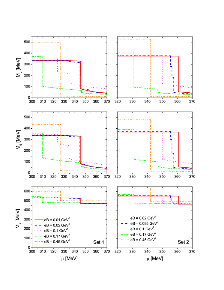
Figure 1: Dressed quark masses as functions of chemical potential for different values of the magnetic field.

We start by analyzing the behavior of the quark constituent masses as functions of the chemical potential for several representative values of the magnetic field shown in Fig.1. Note that here, and in what follows, we use natural units recalling the reader that $eB=1\ \mbox{GeV}^{2}$ corresponds to $B=1.69\times 10^{20}$ G. We consider first the situation for Set 1 (left panels) starting by the lowest chosen value of magnetic field $eB=0.01\ \mbox{GeV}^{2}$ (full red line). As we increase $\mu$ we see that up to certain value $\mu_{c1}=335.3\ \mbox{MeV}$ the dressed masses stay constant. At that point we can observe a (tiny) sudden drop in the masses corresponding to a first order phase transition which goes from the fully chirally broken phase, where the masses are $\mu-$independent, to a less massive one where the masses are $\mu-$dependent. As we continue to increase the chemical potential there is a second tiny jump in the masses (somewhat more easily observed in the plot for $M_{d}$) at $\mu_{c2}=342.3\ \mbox{MeV}$. Increasing $\mu$ further we reach $\mu_{c3}=345.4\ \mbox{MeV}$ where a new, in this case much larger, drop in the masses occur. After this point the dressed $u-$ and $d-$quark masses are much smaller that their vacuum values indicating that light quark sector is in the fully chirally restored phase, namely that if we were to set $m_{u}=m_{d}=0$ (i.e. chiral case) the associated dressed masses would vanish. To identify the different phases it is convenient to adopt the notation of Refs.njl ; pablo . Thus, the fully chirally broken phase in which the system is for $\mu<\mu_{c1}$ is denoted by B. The massive phases in which $M_{f}$ depends on $\mu$ are denoted $\mbox{C}_{i}$ phases. Hence, the system is in the $\mbox{C}_{0}$ phase if $\mu_{c1}<\mu_{c2}$ and in the $\mbox{C}_{1}$ phase if $\mu_{c2}<\mu_{c3}$. The difference between these two phases is that in the $\mbox{C}_{0}$ only the $u-$ and $d-$quark lowest Landau levels (LLL’s) are populated while in $\mbox{C}_{1}$ the $d-$ quark first LL (1LL) also is. It is important to remark that within the range of values of the chemical potential considered in this work no $s-$quark LL is ever populated since this would require larger values of $\mu$. Moreover, the reason why the $d$-quark 1LL is populated without a simultaneous population of the $u$-quark 1LL is due to fact that $|q_{d}|=2|q_{u}|$. For $\mu>\mu_{c3}$ the system is in one of the chirally restored phases $\mbox{A}_{i}$, which differ between themselves in the number of light quark LL’s which are populated. The transitions between these phases correspond to small jumps in the masses (i.e. first order transitions) which in Fig.1 are hardly seen in this case. Considering next the case $eB=0.02\ \mbox{GeV}^{2}$ (blue dashed line) we see that at basically the same value of $\mu_{c1}$ as the one given above there is a first order transition from the B phase to the $\mbox{C}_{0}$ phase. However, in this case no sign of a transition to the $\mbox{C}_{1}$ phase is found as $\mu$ increases. In fact, the following transition corresponds to a big jump in the light quark dressed masses which is associated to the transition between the $\mbox{C}_{0}$ and one of the chiral symmetry restored phases $\mbox{A}_{i}$. It should be noted that this happens at a critical chemical potential which is slightly smaller than the value of $\mu_{c3}$ quoted above. As $\mu$ is further increased consecutive first order transitions between $\mbox{A}_{i}$ occur. Note that the first of them can quite clearly observed in this case. Turning to the case $eB=0.10\ \mbox{GeV}^{2}$ (magenta dotted lines) we see that the overall behavior is similar to that of $eB=0.01\ \mbox{GeV}^{2}$, except for the fact that in the present case the size of the first and second jumps in the masses are quite similar and that they occur at lower values of $\mu$. The situation for $eB=0.17\ \mbox{GeV}^{2}$ (green dash dotted lines) is somewhat peculiar. After a first large jump in the masses (occurring at an even lower value of $\mu$ than the previous cases) they decrease continuously for a rather wide interval of values of $\mu$ which ends with a transition which is characteristic of those between $\mbox{A}_{i}$ phases. Whether in that intermediate interval the system is always in the same phase (of $\mbox{A}_{i}$ type) or it stays first in the $\mbox{C}_{0}$ phase performing at some point a crossover transition to a $\mbox{A}_{i}$ type phase is a question that requires further analysis and is addressed below. Finally, for $eB=0.45\ \mbox{GeV}^{2}$ (orange dash dot dotted lines) the behavior of the system as $\mu$ increases becomes much simpler. There is one single first order phase transition which connects the B and $\mbox{A}_{0}$ phases. Note, however, that this transition occurs at a higher chemical potential as compared to that required in the previous case to induce a transition from the B phase. Turning our attention to the results concerning Set 2 (right panels in Fig.1) we observe that, although for $eB=0.45\ \mbox{GeV}^{2}$ (orange dash dot dotted lines) the behavior is very similar as the corresponding one for Set 1, at low values of $eB$ there are significant differences. For example for $eB=0.02\ \mbox{GeV}^{2}$ (full red lines) the first transition already connects the B phase with one of the $\mbox{A}_{i}$ ones, i.e. there is no sign of an intermediate $\mbox{C}_{0}$ here. As it turns out such a phase only exists for a narrow interval of values of $eB$ of which we take $eB=0.085\ \mbox{GeV}^{2}$ (dashed blue line) as a typical example.

In Fig.2 we show the $eB-\mu$ phase diagrams obtained with both parameter sets. The full lines correspond to first order phase transitions while the dashed and dotted ones to smooth crossovers. As mentioned above the later typically connect some of the $C_{i}$ and $A_{i}$ phases and their determination requires a detailed analysis. In the first place we should stress that, as well known, there is not a unique way to define a crossover transition. In the case of SU(2) cold quark matter under strong magnetic fields this issue was discussed in some detail in Ref.pablo . Following that reference we base our analysis on the chiral susceptibilities introduced at the end of the previous section. In particular, we define the crossover transition line as the ridge occurring in the chiral susceptibility when regarded as a two dimensional function of $eB$ and $\mu$. Mathematically, it can be defined by using for each value of the susceptibility (starting from its maximum value in the given region) the location of the points at which the gradient in the $eB-\mu$ plane is smaller. As remarked in Ref.pablo , this definition must be complemented with the condition that on each side of the curve there should exist at least one region such that there is a maximum in the susceptibility for an arbitrary path connecting both regions. It is important to note that, differently from the $SU(2)$ case discussed in that reference where one single chiral susceptibility can be defined for the two light flavors, the values of $\chi_{u}$ and $\chi_{d}$ at a given point in the $eB-\mu$ plane are in general different in the present case fot . Therefore, there is no reason why there should be identical crossover lines for the two light quark sectors. In fact, and in contrast to what happens with the first order transitions which always coincide, the result of our analysis indicate that for the parametrizations considered this is never the case. As a consequence of this there might be regions in the $eB-\mu$ plane where the $u-$quark sector is in a $\mbox{C}_{i}$ phase and the $d-$quark sector in a $\mbox{A}_{i}$ one and viceversa. In Fig.2, those regions have been indicated by including the notation for each of the corresponding phases (i.e. one for each light quark sector) between brackets. Thus, for example, $[\mbox{A}^{u}_{0},\mbox{C}^{d}_{0}]$ corresponds to a region in which the $u-$ quark sector is in the $\mbox{A}_{0}$ phase and the $d-$ quark sector $\mbox{C}_{0}$. From Fig.2 it is clear that the most remarkable difference between the phase diagrams associated to the two parametrizations considered concerns the regions in which the phases $\mbox{C}_{i}$ exist. For Set 1 the $\mbox{C}_{0}$ phase covers a rather large area of the plane, which in the $eB$ direction extends from very low values up to $eB\simeq 0.15\mbox{GeV}^{2}$ where it has a smooth crossover boundary with the phase $A_{0}$. Note that such a boundary is somewhat different for the two light quark sectors giving rise to an intermediate $[\mbox{A}^{u}_{0},\mbox{C}^{d}_{0}]$ region. Moreover, for this parameter set a small region of $\mbox{C}_{1}$ phase exists for low values of $eB$. In the case of Set 2, however, the phase $\mbox{C}_{0}$ only exists in a small triangular region surrounded by first order transition lines although a small $[\mbox{A}^{u}_{0},\mbox{C}^{d}_{0}]$ region is also present. Another point that it is interesting to address regards the similarities between the present phase diagrams and those reported in Ref.pablo for the SU(2) case with maximum flavor mixing. In fact, the phase diagram obtained for Set 1 has strong similarities to that shown for $M_{0}=340\ \mbox{MeV}$ shown in Fig.12 of that reference. Moreover, that of Set 2 appears to correspond to one somewhere in between those of $M_{0}=360\ \mbox{MeV}$ and $M_{0}=380\ \mbox{MeV}$ of that figure. Interestingly, the vacuum values of the $u-$ and $d-$ dressed quark masses in the vacuum and in the absence of a magnetic field are $M_{u}=M_{d}=336(368)$ MeV for Set 1 (Set 2). Thus, it appears that even in the $SU(3)$ case under consideration the general features of the $eB-\mu$ diagram are dictated to a great extent by the values of light quark dressed quark masses in the vacuum and in the absence of a magnetic field.

We end this section by analyzing in the context of the present SU(3) NJL model the magnetic catalysis (MC) effect mentioned in the Introduction and how this effect is modified by the presence of finite chemical potential leading, for example, to the existence of the so-called inverse magnetic catalysis (IMC) as it has been recently discussed in the literature Preis:2010cq . Actually, the later is usually related to a decrease of the critical chemical potential at intermediate values of the magnetic fields. Such a phenomenon is clearly observed in the phase diagrams displayed in Fig.2. In fact, we see that after staying fairly constant up to $eB\simeq 0.05\ \mbox{GeV}^{2}$ the lowest first order transition line bends down reaching a minimum at $eB\simeq 0.2-0.3\ \mbox{GeV}^{2}$ after which it rises indefinitely with the magnetic field. This implies that, in general, there is some interval of values of the chemical potential for which an increase of the magnetic field at constant $\mu$ causes first a transition from the massive phase B to a less massive phase ($\mbox{C}_{i}$ or $\mbox{A}_{i}$) and afterwards from the massless phase $\mbox{A}_{0}$ back to massive phase B. To address these issues we display in Fig.3 the behavior of the masses as function of magnetic fields for several chemical potentials, and our two parameter sets. In particular, the complex phase structure for Set 1 (left panels) accounts for the different possible behaviors depending on the chemical potential. For $\mu=300$ MeV (red full line), the system is in the B phase for the whole range of magnetic fields, and the MC effect is clearly seen. For $\mu=325$ MeV (magenta dashed line), a similar behavior is seen, except for a middle section where the system passes through a $\mbox{C}_{0}$ phase and an $\mbox{A}_{0}$ phase before returning to the vacuum phase again. Note that when masses are plotted as functions of $eB$, the existence of a crossover transition from $\mbox{C}_{0}$ to $\mbox{A}_{0}$ becomes more noticeable. As already discussed, a detailed analysis shows that the associated critical magnetic field for $u-$quark sector is somewhat lower than that for $d-$quark sector. In this region of the curve, as well as in the rest of the following curves, the effect of IMC is also present. In fact, as already remarked in Ref.pablo , we can conclude that within the $C_{i}$ and $A_{i}$ phases the dressed light quark masses are basically decreasing functions of the magnetic field, while MC occurs principally in the B phase. In particular, for $\mu=340$ MeV (blue dot dotted lines), the phase remains in $\mbox{C}_{0}$ for a significant range of magnetic fields and the mass decreases continuously. Finally, for $\mu=360$ MeV (green dash dotted lines) at low and medium magnetic fields the system goes from a $\mbox{A}_{i}$ phase to another one with $i^{\prime}=i-1$ as the magnetic fields increases, the transition between them being signalled by the peaks in the dressed masses. Eventually, for sufficiently large magnetic fields, it has a first order transition to the B phase. As shown in the right panels of Fig.3, for Set 2 the situation is somewhat simpler. This is, of course, related to the absence of extended $\mbox{C}_{i}$ regions in the associated phase diagram.

IV Final remarks

In the present work we have revisited the phase structure of the magnetized cold quark matter within the framework of the SU(3) NJL model for two parameter sets often used in the literatureBuballa . Although the general pattern is similar, the quantitative results are certainly parameter dependent, as in the case of the SU(2) NJL ebert ; pablo . We have checked that Set 1, i.e. the one leading to lower vacuum values for the dressed quark masses in the absence of a magnetic field, presents a richer phase diagram, with more intermediate phases than Set 2. This is a reflex of the number of small jumps appearing in the quark dressed masses, which are related to the number of filled Landau levels. It is worth emphasizing that, differently from the case of standard SU(2) NJL model with maximum flavor mixing studied in Ref.pablo , within the present version of the SU(3) NJL model the $u-$ and $d-$dressed quark masses, as well as the corresponding condensates, are not necessarily equal for the same chemical potential $\mu$ and magnetic field $B$. As a consequence, three different susceptibilities (one for each flavor) can be defined which, in principle, might bear peaks at different points. This points towards the possibility of having a different crossover transition line for each of three quark flavors. In fact, and in contrast to what happens with the first order transitions which are always found to coincide, the result of our analysis indicate that for the parametrizations considered this is always the case. Hence, the corresponding phase diagrams turn out to have some (small) regions where the quarks of different flavor are in different phases.

The phenomenon of inverse magnetic catalysis as defined in Ref.Preis:2010cq , i.e. the decrease of the critical chemical potential at specific values of the magnetic field intensity, is clearly observed within the present choice of parameters for the SU(3) NJL model. In connection with this, we also note that the response of light quark dressed masses to an increase of the magnetic at fixed $\mu$ depends on the region of $eB-\mu$ phase diagram considered. On the one hand, the increase in light quark dressed masses with magnetic field, known as magnetic catalysis, is principally seen in the vacuum phase B, where chiral symmetry is fully broken. On the other hand, phases where some light quark levels are populated ($\mbox{C}_{i}$ and $\mbox{A}_{i}$) show a dominant decrease in the corresponding masses as magnetic field increased.

We conclude by noting that while in the present work we have restricted ourselves to symmetric quark matter, the role played by charge neutrality and $\beta$-equilibrium in the behavior of quark matter subject to strong magnetic fields is clearly a topic of great interest njlB in the study of magnetars. As the existence of the critical end point is related to the amount of different quark flavors in the system pedro2013 , the resulting phase diagram will certainly be different, and at least at low temperatures, it should be investigated.

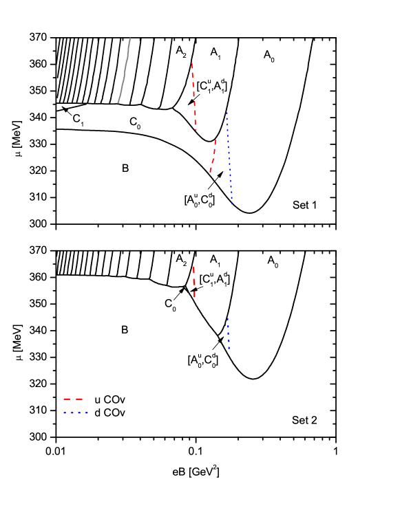
Figure 2: Phase diagrams in the $eB-\mu$ for the set of parameters defined in Table I.

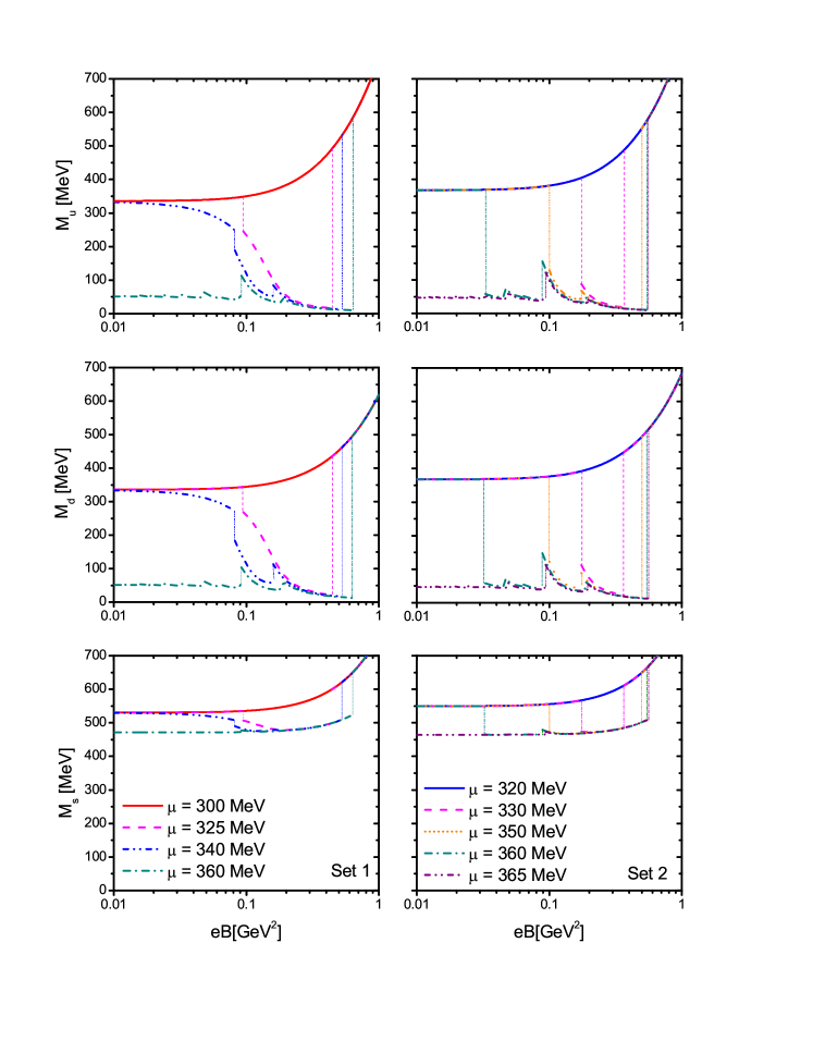
Figure 3: Dressed quark masses as functions of magnetic field for different values of the chemical potential.