On the Construction of Geometric Parameters for
Preferential Fluid Flow Information in Fissured Media

Abstract

For a fissured medium, we analyze the impact that the geometry of the cracks, has in the phenomenon of preferential fluid flow. Using finite volume meshes we analyze the mechanical energy dissipation due to gravity, curvature of the surface and friction against its walls. We construct parameters depending on the Geometry of the surface which are not valid for direct quantitative purposes, but are reliable for relative comparison of mechanical energy dissipation. Such analysis yields Information about the preferential flow directions of the medium which, in most of the cases is not deterministic, therefore the respective Probability Spaces are introduced. Finally, we present the concept of Entropy linked to the geometry of the surface. This notion follows naturally from the random nature of the Preferential Flow Information. fissured media, energy dissipation, preferential flow, probability measures, geometric entropy.
2000 Math Subject Classification: 76S05, 97M99, 94A17

1 Introduction

It is observed from experience, that the phenomenon of fluid flow through porous media is not uniform in every direction, on the contrary, preferential paths are developed. The problem of preferential flow has been extensively studied in recent years from several points of view and at different scales of modeling, due to its remarkable importance in different fields such as oil extraction, water supply, pollution of subsurface streams and soils, waste management, etc. At the pore scale, the presence of solutes and colloids, chemical reactions, high viscosity of the fluid and saturation level have been included in different theoretical and/or empirical models; see JensenHansenMagid ; HagerdornMohn . Nevertheless, upscaling this effects to that of the geological medium, or field scale, has proved to be an extremely difficult task. A different approach emphasizes on the multiple scale aspects of the problem, when preferential flow occurs because of the presence of large pores (connected or not) or geological strata; which generates regions of fast and slow flow exchanging fluid. Hence, several models of coupled systems of partial differential equations have been proposed, such as dual VisaShow ; Barenblatt ; ArbogastDouglasHornung and multiple porosity models SpagnuoloWright , microstructure models Show97 and the coupling of laws at different scale: see ArbLehr2006 for an analytic approach of a Darcy-Stokes system and see LesinigoAngeloQuarteroni for a numerical treatment to a Darcy-Brinkman system. On a different line there are several works, numerical Mclaren ; ArbBrunson2007 or numerical/analytical WangFengHan , dealing with the discretization and numerical aspects as well as the assessment and simulation of the proposed models. Yet another approach lies on a probabilistic point of view FioriJankovic ; BerylandGolden ; Golden based on principles of conductivity. In this work we focus on the impact that the Geometry of the cracks in a fissured medium has on this phenomenon.

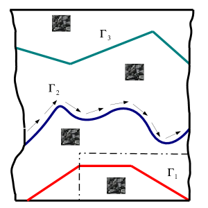
(a) Fissured Medium

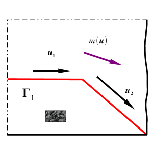
(b) Average Velocity on Fissured System Region

Figure 1: Fissured Medium and Average Velocities

Fissured media are common geological structures, here the fast flow occurs on the cracks while the rock matrix constitutes the slow flow region. For small values of the Reynolds number it is intuitive to see that the saturated flow on the fissures is predominantly parallel to the surface hosting it, see figure 1 (a). This fact has been shown in several rigorous mathematical works, see ArbogastDouglasHornung ; WalkingtonShowalter for homogenization techniques and SpagnuoloCoffield ; Morales ; MoralesShow2 for asymptotic analysis. In the present work we exploit this fact to compute the “average direction” of tangential velocity fields hosted on a surface to predict the likely preferential flow directions of the system. In figure 1 (b) a region of the fissured system is isolated in a way that contains only one crack. Assuming the flow is isotropic on the rock matrix, it follows that the preferential flow direction in this region strictly depends on the flow field hosted on the surface, i.e. its “average” behavior. In this work we assume the medium has one single fissure $\Gamma$ and state that its preferential flow is the “average” tangential flow hosted on the surface $\Gamma$ of the crack. Towards the end of the exposition (section 5.3), it will be clear how to extend the method to a system with multiple fissures.

Describing the exact flow field on the fissures on one hand, has a complexity level essentially equivalent to solving the problem of preferential direction itself, on the other hand for computational purposes it is always necessary to discretize the surface together with the flow fields. Consequently we choose a different approach: first we assume the medium has one single car we construct idealized flow fields related to finite triangulations of a surface, defined only by certain aspects of the geometry of the surface. Such fields are not realistic for describing the flow configuration on the manifold, however they are useful to compare quantities of mechanical energy dissipation. Hence, in order to find the preferential flow directions amongst all the possible aforementioned flow fields, we apply the reasoning line of the Arquimedian weight comparison method. As it turns out, in most of the cases the preferential flow direction is not unique, and a probabilist treatment must be adopted.

Next, we introduce the notation, vectors in $\bm{\mathbbm{R}}^{\!2}$ and $\bm{\mathbbm{R}}^{\!3}$ will be denoted with bold characters and $|\cdot|$ stands for the Euclidean norm. If $\mathbf{x}=(x_{1},x_{2},x_{3})\in\bm{\mathbbm{R}}^{\!3}$ we denote $\widetilde{x}=(x_{1},x_{2})$, and $\mathbf{x}=(\widetilde{x},x_{3})$. The notation $m(\cdot)$ indicates computation of average according to the context. The unitary circle in $\bm{\mathbbm{R}}^{\!2}$ is denoted by $S^{1}$ and the unitary sphere in $\bm{\mathbbm{R}}^{!3}$ is denoted by $S^{2}$. For a given set $A$ we denote $|A|$ its 2-D or 1-D Lebesgue measure in both cases, since it will be clear from the context and $\#A$ stands for its cardinal. The paper is organized as follows: in sections 2, 3 and 4 the preferential flow phenomenon is analyzed from the perspectives of Curvature, Gravity and Friction respectively. All of them are based on comparing mechanical energy dissipation, therefore each section begins constructing adequate flow fields to quantify these losses. Next, the exposition moves to a rigorous discussion of mathematical aspects of the model; most of them necessary for a successful construction of the Preferential Flow Directions Probability Space. Section 5 shows how to assemble the effects previously analyzed and defines the entropy of the preferential flow information; then closes with final remarks and future work. In the reminder of this section we present the geometric setting and the minimum necessary background from fluid mechanics.

1.1 Geometric Setting and Triangulation of the Surface

This work will be restricted to the treatment of surfaces $\Gamma$ coming from a piecewise $C^{1}$-function $\zeta:G\rightarrow\bm{\mathbbm{R}}$ defined on an open bounded simply connected set $G$ of $\bm{\mathbbm{R}}^{\!2}$. In particular the piecewise $C^{1}$ 2-D manifold $\Gamma$ has an Atlas containing one element. The approximation of surfaces will be done by piecewise linear affine triangulations. However, the triangulation has to meet certain geometric conditions in order to be suitable for later quantifications of mechanical energy losses. Those conditions are consistent with the concept of admissible mesh in the sense of GallouetHerbin ; BradjiHerbin (Definition 9.1 page 762); we have

Definition 1.1.

Let $\Omega$ be an open bounded polygonal subset of $\bm{\mathbbm{R}}^{d}$, $d=2,3$. An admissible finite volume mesh of $\Omega$, denoted by $\mathcal{T}$, is given by a family of “control volumes” $\{K:K\in\mathcal{T}\}$, which are open polygonal convex subsets of $\Omega$, a family of subsets of $cl(\Omega)$ contained in hyperplanes of $\bm{\mathbbm{R}}^{d}$, denoted by $\mathcal{E}$ (these are the edges in two dimensions or faces in three dimensions of the control volumes), with strictly positive $(d-1)$-dimensional measure, and a family of points, of $\Omega$ denoted by $\mathcal{P}$ satisfying the following properties:

1. $cl(\Omega)=cl\bigcup_{K\in\mathcal{T}}K$

2. For any $K\in\mathcal{T}$, there exists a subset $\mathcal{E}_{K}$ of $\mathcal{E}$ such that $\partial K=cl(K)-K=\bigcup_{\sigma\in\mathcal{E}_{K}}cl(\sigma)$. Furthermore, $\mathcal{E}=\bigcup_{K\in\mathcal{T}}\mathcal{E}_{K}$.

3. For any $(K,L)\in\mathcal{T}^{\,2}$ with $K\neq L$, either the $(d-1)$-dimensional Lebesgue measure of $cl(K)\cap cl(L)$ is 0 or $cl(K)\cap cl(L)=cl(\sigma)$ for some $\sigma\in\mathcal{E}$, which will then be denoted by $K|L$.

4. The family $\mathcal{P}=\{x_{K}:K\in\mathcal{T}\}$ is such that $x_{K}\in cl(K)$ (for all $K\in\mathcal{T}$) and if $\sigma=K|L$, it is assumed that $x_{K}\neq x_{L}$, and that the straight line $\mathcal{D}_{K,L}$ going through $x_{K}$ and $x_{L}$ is orthogonal to $K|L$.

5. For any $\sigma\in\mathcal{E}$ such that $\sigma\subset\partial\Omega$, let $K$ be the control volume such that $\sigma\in\mathcal{E}_{K}$. If $x_{K}\notin\sigma$, let $\mathcal{D}_{K,\sigma}$ be the straight line going through $x_{K}$ and orthogonal to $\sigma$, then the condition $\mathcal{D}_{K,\sigma}\cap\sigma\neq\emptyset$ is assumed. Define

   $$y_{\sigma}\overset{\textbf{def}}{=}\mathcal{D}_{K,\sigma}\cap\sigma$$ (1)

From now on we adopt triangular meshes as provided in GallouetHerbin

Definition 1.2.

Let $\Omega$ be an open bounded polygonal subset of $\bm{\mathbbm{R}}^{2}$. We say a triangular mesh is a family $\mathcal{T}$ of open triangular disjoint subsets of $\Omega$ such that two triangles having a common edge have also two common vertices and such that all the interior angles of the triangles are less than $\frac{\pi}{2}$.

Clearly a triangular mesh described in the definition above meets the conditions of 1.1. In particular, the condition on the interior angles assures that the orthogonal bisectors intersect inside each triangle, thus naturally defining the points $x_{K}\in K$. Since definitions 1.1 and 1.2 demand a polygonal domain we introduce the collection of eligible polygons.

Definition 1.3.

Let $\Gamma=\{[\widetilde{x},\zeta(\widetilde{x})]:\widetilde{x}\in G\}$ be a piecewise $C^{1}$ surface. We say a polygonal domain is eligible for triangulation of $\Gamma$ if it is contained in $G$ and if its vertices lie on the boundary of $G$. From now on we denote $Poly\,(G)$ the family of all such polygons.

Now we introduce a central definition for the type of triangulations to be worked on

Definition 1.4.

Let $\Gamma=\{[\widetilde{x},\zeta(\widetilde{x})]:\widetilde{x}\in G\}$ be a piecewise $C^{1}$ surface and $K$ a triangular domain contained in $G$ with vertices $\{z_{\,\ell}:1\leq\ell\leq 3\}\subset\bm{\mathbbm{R}}^{2}$ we define its “lifting” as the closed convex hull of the points $\{[z_{\,\ell},\zeta(z_{\,\ell})]:1\leq\ell\leq 3\}\subset\bm{\mathbbm{R}}^{3}$. We denote this surface by $K^{\zeta}$ and the outer unitary vector perpendicular to it by $\bm{\widehat{n}}(K)$.

Next we define a Triangulation of the surface $\Gamma$.

Definition 1.5.

Let $\Gamma$ be a piecewise $C^{1}$ surface, $\mathcal{H}\in Poly\,(G)$ and $\mathcal{T}$ an admissible triangular mesh of $\mathcal{H}$ as in definition 1.2.

1. We say the triangulation of $\Gamma$ relative to the polygon $\mathcal{H}$ and the mesh $\mathcal{T}$, is given by the “lifting” $K^{\zeta}$ of each element $K$ of$\mathcal{T}$. We denote

   $$\Gamma_{\scriptscriptstyle\mathcal{H},\,\mathcal{T}}\overset{\textbf{def}}{=}\bigcup\left\{K^{\zeta}:K\in\mathcal{T}\right\}$$ (2)

2. The point of control $\mathbf{p}^{K}$ is given by the unique point in $K^{\zeta}$ such that its horizontal projection agrees with $x_{K}$, the circumcenter of $K$ i.e.

   $$\mathbf{p}^{K}-(\mathbf{p}^{K}\cdot\bm{\widehat{k}})\,\bm{\widehat{k}}=x_{K}$$ (3)

   Moreover $\mathbf{p}^{K}$ is the “lifting” of $x_{K}$.

3. Given an edge $\sigma\in\mathcal{E}$ and its middle point $y_{\sigma}$, the associated “transmission point” is the unique point $\mathbf{q}^{\sigma}$ contained in $\Gamma_{\mathcal{H},\mathcal{T}}$ such that

   $$\mathbf{q}^{\sigma}-(\mathbf{q}^{\sigma}\cdot\bm{\widehat{k}})\,\bm{\widehat{k}}=y_{\sigma}$$ (4)

   i.e. $\mathbf{q}^{\sigma}$ is the “lifting” of $y_{\sigma}$.

4. Define $\mathcal{E}_{int}\overset{\textbf{def}}{=}\{\sigma\in\mathcal{E}:|\sigma\cap\partial\mathcal{H}|=0\}$ i.e. the set of interior edges of the triangulation $\mathcal{T}$.

5. For each element $K\in\mathcal{T}$ define its edge-influence triangles as the three subtriangles generated by drawing rays from $x_{K}$ to each of its vertices. Figure 2 depicts the lifting of two neighboring elements $K$ and $L$, its common edge $\sigma=K|L$ and the corresponding edge-influence triangles.

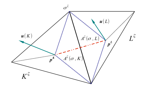
Figure 2: Edge Influence $\&$ Configuration

1.2 The Strain Rate Tensor and Mechanical Energy Loss

For the sake of completeness we recall the definition of strain rate tensor Batchelor . Given a differentiable flow field $\mathbf{v}:G\rightarrow\bm{\mathbbm{R}}^{d}$, $G$ open set in $\bm{\mathbbm{R}}^{d}$, the strain rate tensor $D(\mathbf{v}):G\rightarrow\bm{\mathbbm{R}}^{d\times d}$ is given by

$$D_{j,\ell}(\mathbf{v})\overset{\textbf{def}}{=}\frac{1}{2}\left(\frac{\partial\mathbf{v}_{j}}{\partial x_{\ell}}+\frac{\partial\mathbf{v}_{\ell}}{\partial x_{j}}\right),\quad 1\leq j,\,\ell\leq d$$ (5)

Finally, the internal deformation energy of a viscous fluid is given by Bear

$$E=\frac{2\,\mu}{\rho}\,D(\mathbf{v}):D(\mathbf{v})\overset{\textbf{def}}{=}\frac{2\,\mu}{\rho}\sum_{j,\ell}\left|D_{j,\ell}(\mathbf{v})\right|^{2}$$ (6)

Where $\mu$ represents the viscosity and $\rho$ the density of the fluid.

2 Preferential Flow due to Curvature

2.1 Flow Hypothesis

We want to compute a conservative tangential flow field, hosted within the surface $\Gamma$ and totally defined by its curvature. As already specified in the introduction, this paper will be restricted to the construction of a discretized flow field related to a triangulation $\Gamma_{\scriptscriptstyle\mathcal{H},\,\mathcal{T}}$. The changes on the flow field must be exclusively due to the changes of directions on the elements of the surface $\Gamma_{\scriptscriptstyle\mathcal{H},\,\mathcal{T}}$. Then, for simplicity we choose the following defining properties

1. The velocity must be constant in magnitude and direction within a flat face.

2. The magnitude of the velocity must be constant on every part of the surface.

3. The field must meet the continuity flow condition i.e. on the edge where two different faces intersect the component of the velocities perpendicular to the edge must have the same magnitude.

For the construction of such velocity field we introduce a velocity of reference or master velocity which will be denoted $\mathbf{u}^{\Gamma}$. Since the surface $\Gamma$ is defined by a $C^{1}(G)$ function, no triangulation $\Gamma_{\mathcal{H},\,\mathcal{T}}$ contains vertical faces, i.e. $\bm{\widehat{n}}(K)\cdot\bm{\widehat{k}}\neq 0$ for all $K\in\mathcal{T}$. Hence, whichever tangential flow that the surface $\Gamma_{\mathcal{H},\,\mathcal{T}}$ hosts has a non-null projection onto the plane $\langle\bm{\widehat{k}}\rangle^{\perp}$. Consequently, it is enough to assume that the velocity of reference $\mathbf{u}^{\Gamma}$ is hosted in the horizontal plane.

2.2 Construction of the Velocity Field

Let $\Gamma$ be a piecewise $C^{1}$ surface and $\Gamma_{\scriptscriptstyle\mathcal{H},\mathcal{T}}$ be a triangulation. Given a reference velocity $\mathbf{u}^{\Gamma}$ we are to build the velocity $\mathbf{u}(K)$ on the element $K^{\zeta}$(the lifting of $K$). If $K^{\zeta}$ is horizontal i.e if $\bm{\widehat{n}}(K)\equiv\bm{\widehat{k}}$ we simply set $\mathbf{u}(K)=\mathbf{u}^{\Gamma}$. For the non-trivial case when $K^{\zeta}$ is not horizontal ($\bm{\widehat{n}}(K)\times\bm{\widehat{k}}\neq 0$), we proceed as follows. In the figure 3 below we illustrate the relation between velocities. It depicts the horizontal and vertical view of the intersection between the plane $\langle\bm{\widehat{k}}\rangle^{\perp}$ and the plane containing $K^{\zeta}$ an element of $\Gamma_{\mathcal{H},\,\mathcal{T}}$.

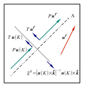
(a) Horizontal View

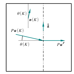
(b) Vertical View

Figure 3: Intersection $K^{\zeta}\cap\langle\bm{\widehat{k}}\rangle^{\perp}$

On the left hand side of figure 3 we have the reference velocity $\mathbf{u}^{\Gamma}$ and a decomposition of the local velocity $\mathbf{u}(K)$. The fine dashed line in the direction of the unitary vector $\xi^{K}\overset{\textbf{def}}{=}|\bm{\widehat{n}}(K)\times\bm{\widehat{k}}|^{-1}\,\bm{\widehat{n}}(K)\times\bm{\widehat{k}}$ represents the intersection line of the plane containing $K^{\zeta}$ and the plane $\langle\bm{\widehat{k}}\rangle^{\perp}$. We decompose $\mathbf{u}^{\Gamma}$ in two vectors lying on the horizontal plane $\langle\bm{\widehat{k}}\rangle^{\perp}$, one parallel to the intersection line $\langle\xi^{K}\rangle$ and the other perpendicular to it i.e.

$$T(K)\,\mathbf{u}^{\Gamma}=T\,\mathbf{u}^{\Gamma}\overset{\textbf{def}}{=}\left(\mathbf{u}^{\Gamma}\cdot\xi^{\,K}\right)\xi^{\,K},\\$$ (7a)

$$P(K)\,\mathbf{u}^{\Gamma}=P\,\mathbf{u}^{\Gamma}\overset{\textbf{def}}{=}\mathbf{u}^{\Gamma}-\left(\mathbf{u}^{\Gamma}\cdot\xi^{\,K}\right)\xi^{\,K},$$ (7b)

$$\mathbf{u}^{\Gamma}=T\,\mathbf{u}^{\Gamma}+P\,\mathbf{u}^{\Gamma}.$$ (7c)

Since the component $T\,\mathbf{u}^{\Gamma}$ belongs to the intersection of both planes $\langle\bm{\widehat{k}}\rangle^{\perp}\cap\langle\bm{\widehat{n}}(K)\rangle^{\perp}$, we set it equal to the component of $\mathbf{u}(K)$ in the same direction i.e.

$$T(K)\,\mathbf{u}(K)\overset{\textbf{def}}{=}T(K)\,\mathbf{u}^{\Gamma}$$ (8)

On the right hand side of figure 3 we depict the trace through the vertical plane $\Lambda\overset{\textbf{def}}{=}\langle\xi^{\,K}\rangle^{\perp}$. Denote $P(K)\,\mathbf{u}(K)$ the component of $\mathbf{u}(K)$ perpendicular to $\xi^{\,K}$, we set this component to be a rotation of $P(K)\,\mathbf{u}^{\Gamma}$ by the angle $\theta(K)$, strictly contained in the plane $\langle\xi^{\,K}\rangle^{\perp}$; where the angle $\theta(K)$ is equal to the angle formed between $\bm{\widehat{k}}$ and $\bm{\widehat{n}}(K)$. Notice that the map $\mathbf{u}^{\Gamma}\in\bm{\mathbbm{R}}^{\!2}\mapsto\mathbf{u}(K)$ for fixed $K^{\zeta}\in\Gamma_{\scriptscriptstyle\mathcal{H},\,\mathcal{T}}$ is linear, therefore writing $\mathbf{u}^{\Gamma}=\alpha_{\,1}\,\bm{\widehat{\imath}}+\alpha_{\,2}\,\contour[2]{black}{$\widehat{\jmath}$}$ a direct calculation yields

$$\mathbf{u}(K)\equiv\left(\begin{array}[]{cc}1-\dfrac{\bm{\widehat{n}}_{1}^{\,2}}{1+\bm{\widehat{n}}_{\,3}}&-\dfrac{\bm{\widehat{n}}_{1}\,\bm{\widehat{n}}_{\,2}}{1+\bm{\widehat{n}}_{\,3}}\\[8.0pt] -\dfrac{\bm{\widehat{n}}_{1}\,\bm{\widehat{n}}_{\,2}}{1+\bm{\widehat{n}}_{\,3}}&1-\dfrac{\bm{\widehat{n}}_{\,2}^{\,2}}{1+\bm{\widehat{n}}_{\,3}}\\[8.0pt] \bm{\widehat{n}}_{1}&\bm{\widehat{n}}_{\,2}\end{array}\right)\left\{\begin{array}[]{c}\alpha_{\,1}\\[20.0pt] \alpha_{\,2}\end{array}\right\}\\ \overset{\textbf{def}}{=}\left(V_{\Gamma_{\mathcal{H},\,\mathcal{T}}}\mathbf{u}^{\Gamma}\right)(K).$$ (9a)

Where $$\bm{\widehat{n}}(K)=\bm{\widehat{n}}_{1}\bm{\widehat{\imath}}+\bm{\widehat{n}}_{2}\contour[2]{black}{$\widehat{\jmath}$}+\bm{\widehat{n}}_{3}\bm{\widehat{k}} V_{\Gamma_{\mathcal{H},\,\mathcal{T}}}\mathbf{u}^{\Gamma}:\mathcal{H}\rightarrow\bm{\mathbbm{R}}^{\!3}$$ . The global velocity field is defined by

$$V_{\Gamma_{\mathcal{H},\,\mathcal{T}}}\mathbf{u}^{\Gamma}(s)\overset{\textbf{def}}{=}\sum_{K\in\mathcal{T}}\mathbf{u}(K)\,\bm{\mathbbm{1}}_{K}(s)\,,\quad s\in\mathcal{H}$$ (9b)

Remark 2.1.

1. By construction it is clear that the field in the expression (9) meets the criteria (i), (ii) and (iii) of the flow hypothesis described at the begining of section 2.1.

2. Observe that if $K^{\zeta}$ is horizontal, then $\mathbf{u}(K)=\mathbf{u}^{\Gamma}$ as expected i.e. the expression (9) covers all the possible cases.

3. Whenever there is no ambiguity we will simply denote $\mathbf{u}=V_{\Gamma_{\mathcal{H},\,\mathcal{T}}}\mathbf{u}^{\Gamma}$.

For the field of velocity given by expression (9) we define the average velocity in the natural way

$$m(V_{\Gamma_{\mathcal{H},\,\mathcal{T}}}\mathbf{b})\overset{\textbf{def}}{=}\sum_{K\,\in\,\mathcal{T}}\frac{|K^{\zeta}|}{|\Gamma_{\mathcal{H},\,\mathcal{T}}|}\,\left(V_{\Gamma_{\mathcal{H},\,\mathcal{T}}}\mathbf{b}\right)(K)$$ (10)

Clearly, the map $m\circ V_{\Gamma_{\mathcal{H},\,\mathcal{T}}}:\bm{\mathbbm{R}}^{2}\rightarrow\bm{\mathbbm{R}}^{3}$ is linear. It is important to stress that $m(V_{\Gamma_{\mathcal{H},\,\mathcal{T}}}\mathbf{b})$ may not be tangential to (or hosted within) $\Gamma_{\mathcal{H},\,\mathcal{T}}$. Another important fact is the following

Lemma 2.2.

Let $\Gamma$ be a piecewise $C^{1}$ surface, $\Gamma_{\scriptscriptstyle\mathcal{H},\mathcal{T}}$ be a triangulation and the average velocity operator $m$ defined by (10), then

1. $\ker(m\circ V_{\Gamma_{\mathcal{H},\,\mathcal{T}}})=\{\bm{0}\}$.

2. The space $(m\circ V_{\Gamma_{\mathcal{H},\,\mathcal{T}}})(\bm{\mathbbm{R}}^{\!2})$ is two dimensional.

Proof 2.3.

1. Let $\mathbf{b}=\alpha_{1}\bm{\widehat{\imath}}+\alpha_{2}\contour[2]{black}{$\widehat{\jmath}$}$ such that $|\mathbf{b}|=1$ and $K\in\mathcal{T}$ be arbitrary, then

   $$\left(V_{\Gamma_{\mathcal{H},\,\mathcal{T}}}\mathbf{b}\right)(K)\cdot\mathbf{b}=\left(1-\frac{\bm{\widehat{n}}_{1}^{\,2}}{1+\bm{\widehat{n}}_{\,3}}\right)\alpha_{1}^{2}-2\,\frac{\bm{\widehat{n}}_{1}\,\bm{\widehat{n}}_{2}}{1+\bm{\widehat{n}}_{\,3}}\,\alpha_{1}\,\alpha_{2}+\left(1-\frac{\bm{\widehat{n}}_{2}^{\,2}}{1+\bm{\widehat{n}}_{\,3}}\right)\alpha_{2}^{2}\\ =(\alpha_{1}^{2}+\alpha_{2}^{2})-\frac{1}{1+\bm{\widehat{n}}_{\,3}}(\bm{\widehat{n}}_{1}\alpha_{1}+\bm{\widehat{n}}_{2}\alpha_{2})^{2}\geq 1-(|\mathbf{b}||\bm{\widehat{n}}|)^{2}=0$$

   Therefore, the horizontal projection of $\left(V_{\Gamma_{\mathcal{H},\,\mathcal{T}}}\mathbf{b}\right)(K)$ makes an angle with $\mathbf{b}$ less or equal than $\frac{\pi}{2}$. This implies that the projection onto $\mathbf{b}$ satisfies

   $$P_{\scriptscriptstyle\mathbf{b}}\,\left(V_{\Gamma_{\mathcal{H},\,\mathcal{T}}}\mathbf{b}\right)(K)=\lambda\,\mathbf{b}\,,\quad\lambda>0\,,\;\forall\,K\in\mathcal{T}.$$

   Finally, since $\mathbf{b}\neq 0$ and the weighting coefficients in (10) multiplying $\left(V_{\Gamma_{\mathcal{H},\,\mathcal{T}}}\mathbf{b}\right)(K)$ are positive for all $K\in\mathcal{T}$, it follows that $P_{\scriptscriptstyle\mathbf{b}}\left(m_{\scriptscriptstyle\Gamma_{\mathcal{H},\,\mathcal{T}}}(\mathbf{b})\right)\neq\bm{0}$; which concludes the first part.

2. Follows immediately from the previous part and the dimension theorem.

2.3 Dissipation of Mechanical Energy Model due to Curvature

The discrete model of mechanical energy dissipation due to change of direction has to be consistent with the expression (6) i.e. we need to generate a discrete field of strain rate tensors using the velocity given in (9). The flow field can change only from one element of the triangulation to another. Consequently, the variations of the flow field across the edges define the strain rate tensor we seek.

Definition 2.4.

Let $\sigma\in\mathcal{E}_{int}$ and $K$, $L$ be the two elements of $\Gamma_{\scriptscriptstyle\mathcal{H},\,\mathcal{T}}$ such that $\sigma=K|L$; denote $\mathbf{p}^{K},\mathbf{p}^{L}$ and $\mathbf{u}(K),\mathbf{u}(L)$ the respective points of control and fluid velocity for each element.

1. Define the strain rate tensor across $\sigma$ by

   $$D_{k,\,\ell}(\sigma)\overset{\textbf{def}}{=}\frac{1}{2}\,\frac{\left[\mathbf{u}(K)-\mathbf{u}(L)\right]\cdot\bm{\widehat{e}}_{k}}{\left[\mathbf{p}^{K}-\mathbf{p}^{L}\right]\cdot\bm{\widehat{e}}_{\ell}}+\frac{1}{2}\,\frac{\left[\mathbf{u}(K)-\mathbf{u}(L)\right]\cdot\bm{\widehat{e}}_{\ell}}{\left[\mathbf{p}^{K}-\mathbf{p}^{L}\right]\cdot\bm{\widehat{e}}_{k}}\,,$$ (11a)

   $$D(\sigma)\overset{\textbf{def}}{=}\left\{D_{k,\,\ell}(\sigma):1\leq k,\ell\leq 3\right\}.$$ (11b)

   Here $\bm{\widehat{e}}_{1}=\bm{\widehat{\imath}}$, $\bm{\widehat{e}}_{\,2}=\contour[2]{black}{$\widehat{\jmath}$}$ and $\bm{\widehat{e}}_{3}=\bm{\widehat{k}}$.

2. The strain tensor is extended to the whole surface $\Gamma_{\scriptscriptstyle\mathcal{H},\,\mathcal{T}}$ by

   $$D(s)\overset{\textbf{def}}{=}\sum_{\sigma\,\in\,\mathcal{E}_{int}}D(\sigma)\left[\bm{\mathbbm{1}}_{A(\sigma,K)}+\bm{\mathbbm{1}}_{A(\sigma,L)}\right](s)\,,\quad s\in\mathcal{H}.$$ (12)

   Where $A(\sigma,K)$ and $A(\sigma,L)$ denote the edge-influence triangles of $K$ and $L$ respectively, incident on $\sigma$ given in (v) definition 1.5. Figure 2 displays a horizontal view of two neighboring elements.

Finally, using (12) to compute (6) we have that the global dissipation of energy on the triangulation $\Gamma_{\scriptscriptstyle\mathcal{H},\,\mathcal{T}}$ under the master velocity $\mathbf{u}^{\Gamma}$ is given by

$$U_{curv}(\mathbf{u}^{\Gamma})\overset{\textbf{def}}{=}\frac{2\,\mu}{\rho}\sum_{\sigma\,\in\,\mathcal{E}_{int}}\left\{|A^{\zeta}(\sigma,K)|+|A^{\zeta}(\sigma,L)|\right\}D(\sigma):D(\sigma).$$ (13)

Here $|A^{\zeta}(\sigma,K)|,|A^{\zeta}(\sigma,L)|$ are the areas of the lifted adjacent triangles $A(\sigma,K)$, $A(\sigma,L)$ respectively. Clearly $U_{curv}$ depends only on the triangulation $\Gamma_{\mathcal{H},\,\mathcal{T}}$ and the master velocity $\mathbf{u}^{\Gamma}$.

Remark 2.5.

Given a triangulation $\Gamma_{\scriptscriptstyle\mathcal{H},\,\mathcal{T}}$ of a piecewise $C^{1}$ surface $\Gamma$, denote by $diam(\Gamma_{\scriptscriptstyle\mathcal{H},\,\mathcal{T}})$ the maximum diameter of its elements $K^{\zeta}$. Letting $diam(\Gamma_{\mathcal{H},\,\mathcal{T}})\rightarrow 0$, on one hand, the map $s\in\mathcal{H}\mapsto\sum_{K\in\mathcal{T}}\bm{\widehat{n}}(K)\,\bm{\mathbbm{1}}_{K}$ converges (non-conformally) to $s\in\mathcal{H}\mapsto\bm{\widehat{n}}(s)$ almost everywhere; on the other hand, the distance $|\mathbf{p}^{K}-\mathbf{p}^{L}|$ tends to zero. Due to the definition of the flow field $V_{\Gamma_{\mathcal{H},\,\mathcal{T}}}\mathbf{u}^{\Gamma}$ given in (9), the expression (11) starts approaching values of a directional derivative of the map $s\in\Gamma\mapsto\bm{\widehat{n}}(s)$ (on the points where is differentiable); and the curvature information of the surface $\Gamma$ is contained in these derivatives. Hence, the tensor proposed in (11) and the mechanical energy dissipation proposed in (13) are heavily defined by the curvature (or rather an approximation of the curvature) of the surface $\Gamma$.

2.4 Minimum and Maximum Mechanical Energy Dissipation due to Curvature

By definition the functional $U_{curv}:\bm{\mathbbm{R}}^{2}\rightarrow\bm{\mathbbm{R}}$ is a quadratic form, then it holds that

$$U_{curv}(\mathbf{b})=\mathbf{b}^{T}\,M_{curv}\,\mathbf{b},$$ (14)

for $M_{curv}$ symmetric, positive semi-definite matrix. Due to the spectral theorem, the matrix $M_{curv}$ is orthogonally diagonalizable. Denote $0\leq\lambda_{1}\leq\lambda_{\,2}$ the eigenvalues and $\{\bm{\widehat{f}}_{\!\!\!1},\bm{\widehat{f}}_{\!\!2}\}$ an associated orthonormal basis of eigenvectors, then

$$\begin{split}U_{curv}(\mathbf{b})&=\lambda_{1}\,(\mathbf{b}\cdot\bm{\widehat{f}}_{\!\!\!1})^{2}+\lambda_{\,2}(\mathbf{b}\cdot\bm{\widehat{f}}_{\!\!2})^{2},\\ \lambda_{1}&=\min\{U_{curv}(\mathbf{b}):|\mathbf{b}|=1\}=U_{curv}(\bm{\widehat{f}}_{\!\!\!1}),\\ \lambda_{2}&=\max\{U_{curv}(\mathbf{b}):|\mathbf{b}|=1\}=U_{curv}(\bm{\widehat{f}}_{\!\!\!2}).\end{split}$$ (15)

i.e. the question of minimum and maximum mechanical energy dissipation due to curvature of the surface is equivalent to an eigenvalue problem of $M_{curv}\in\bm{\mathbbm{R}}^{2\times 2}$.

2.5 Preferential Fluid Flow Directions Due to Curvature and Their Probability Space.

The Preferential Fluid Flow Directions of the surface $\Gamma_{\mathcal{H},\,\mathcal{T}}$ due to Curvature are given by

$$\varpi_{curv}\overset{\textbf{def}}{=}\left\{\frac{m(V_{\Gamma_{\mathcal{H},\,\mathcal{T}}}\mathbf{b})}{|m(V_{\Gamma_{\mathcal{H},\,\mathcal{T}}}\mathbf{b})|}:\mathbf{b}\neq\bm{0},\,U_{curv}(\mathbf{b})=\lambda_{1}|\mathbf{b}|^{\,2}\right\}.$$ (16)

Due to lemma 2.2 part i the set $\varpi_{curv}$ is well-defined. It is direct to see that if $\lambda_{1}<\lambda_{2}$ then $\varpi_{curv}$ will have two elements, namely $|m_{\scriptscriptstyle\Gamma_{\mathcal{H},\,\mathcal{T}}}(\bm{\widehat{f}}_{\!\!\!1})|^{-1}m_{\scriptscriptstyle\Gamma_{\mathcal{H},\,\mathcal{T}}}(\bm{\widehat{f}}_{\!\!\!1})$ and $|m_{\Gamma_{\mathcal{H},\,\mathcal{T}}}(-\bm{\widehat{f}}_{\!\!\!1})|^{-1}m_{\Gamma_{\mathcal{H},\,\mathcal{T}}}(-\bm{\widehat{f}}_{\!\!\!1})$ for $\bm{\widehat{f}}_{\!\!\!1}$ the unitary vector associated to $\lambda_{1}$. On the other hand if $\lambda_{1}=\lambda_{2}$ then $\varpi_{curv}$ has infinitely many elements due to lemma 2.2 part ii. In both cases it can not be chosen which direction within $\varpi_{curv}$ is preferential over the others. Due to the uncertainty of this information we must treat it from a Probabilistic point of view. In order to give a consistent definition for the probability space of preferential directions we need to introduce a previous one for technical reasons.

Definition 2.6.

Let $\Gamma$ be a piecewise $C^{1}$ surface, $\Gamma_{\scriptscriptstyle\mathcal{H},\mathcal{T}}$ be a triangulation and $\omega_{curv}=\{\mathbf{b}\in S^{1}:U_{curv}(\mathbf{b})=\lambda_{1}\}$, consider the surjective function

$$\varphi:\omega_{curv}\rightarrow\varpi_{curv}\,,\quad\varphi(\bm{\widehat{e}})\overset{\textbf{def}}{=}\frac{m(V_{\Gamma_{\mathcal{H},\,\mathcal{T}}}\bm{\widehat{e}})}{|m(V_{\Gamma_{\mathcal{H},\,\mathcal{T}}}\bm{\widehat{e}})|}.$$ (17)

Let $\beta$ be the family of all Borel sets of $S^{1}$ intersected with $\omega_{curv}$, define the following $\sigma$-algebra

$$\tau_{curv}\overset{\textbf{def}}{=}\left\{A\in\wp(\varpi_{curv}):\varphi^{-1}(A)\in\beta\right\}.$$ (18)

Where $\wp(\varpi_{curv})$ is the power set of $\varpi_{curv}$.

Finally, we endow the preferential flow space with the uniform probability distribution.

Definition 2.7.

Let $\Gamma$ be a piecewise $C^{1}$ surface, $\Gamma_{\scriptscriptstyle\mathcal{H},\mathcal{T}}$ be a triangulation and $\varpi_{curv}$ be the associated preferential fluid flow directions defined in (16) then

1. If $\lambda_{1}<\lambda_{\,2}$ then $\#\varpi_{curv}=2$; define

   (19)

   Where $\bm{\widehat{f}}_{\!\!\!1}$ is the eigenvector associated to $\lambda_{1}$.

2. If $\lambda_{1}=\lambda_{\,2}$ define

   (20)

   Here $\mu$ indicates the arc-length measure in $S^{1}$.

3 Preferential Flow Due to Gravity

In the present section we address the question of quantifying the impact of gravity on the preferential flow directions, then we require a flow field generated uniquely due to this effect. The problem is approached with a very similar analysis to the one presented in section 2. An appropriate variation on the flow hypothesis and the same construction of finite volume mesh for the triangulation of a piecewise $C^{1}$ surface will be used.

3.1 Flow Hypothesis

For a given triangulation $\Gamma_{\scriptscriptstyle\mathcal{H},\,\mathcal{T}}$ of the surface $\Gamma$, the idealized flow field must experience changes only due to the relative difference of heights of the flat faces of the elements of the triangulation. Hence, it must satisfy the following conditions

1. The velocity is constant in magnitude and direction within a flat face.

2. The magnitude of the velocity within a flat element $K^{\zeta}$ is given by

   $$\left|\mathbf{u}(K)\right|\overset{\textbf{def}}{=}\sqrt{2\,g\,\left(\frac{1}{2\,g}+z_{\max}-\mathbf{p}^{K}\cdot\bm{\widehat{k}}\right)}.$$ (21a)

   Where $$g$$ is the gravity and

   $$z_{\max}\overset{\textbf{def}}{=}\max\left\{\mathbf{p}^{L}\cdot\bm{\widehat{k}}:L\in\mathcal{T}\right\}.$$ (21b)

   The addition of the quantity $\frac{1}{2\,g}$ to the height of reference in the expression (21a) above is meant to have velocities of magnitude $1$ on the volumes of control $L^{\zeta}$ of highest altitude (where the velocity has minimum magnitude).

3. The field must meet the continuity flow condition, therefore the discharge rate $Q_{0}$ must remain constant. Thus, for all $K,L\in\mathcal{T}$ it must hold

   $$w(K)\left|\mathbf{u}(K)\right|=w(L)\left|\mathbf{u}(L)\right|\equiv Q_{0}\overset{\textbf{def}}{=}1.$$ (22)

   Here $w(K)$ indicates the height of the fluid layer on the element $K^{\zeta}$. For simplicity we defined the discharge rate to be $1$.

Remark 3.1.

Observe that in condition (iii) above we needed to introduce the fluid layer height $w(L)$. However it is the reciprocal of the velocity magnitude $|\mathbf{u}(L)|$ i.e. it is not and independent variable.

3.2 The Velocity Field Due to Gravity

Using the construction of the velocity field presented in section 2.2 we have that for a given master velocity $\mathbf{u}^{\Gamma}=\alpha_{\,1}\,\bm{\widehat{\imath}}+\alpha_{\,2}\,\contour[2]{black}{$\widehat{\jmath}$}$ and $K\in\mathcal{T}$, the velocity at the volume of control $K^{\zeta}$ is given by

$$\mathbf{u}(K)\equiv\sqrt{2\,g\left(\frac{1}{2\,g}+z_{\max}-\mathbf{p}^{L}\cdot\bm{\widehat{k}}\right)}\left(\begin{array}[]{cc}1-\dfrac{\bm{\widehat{n}}_{1}^{\,2}}{1+\bm{\widehat{n}}_{\,3}}&-\dfrac{\bm{\widehat{n}}_{1}\,\bm{\widehat{n}}_{\,2}}{1+\bm{\widehat{n}}_{\,3}}\\[8.0pt] -\dfrac{\bm{\widehat{n}}_{1}\,\bm{\widehat{n}}_{\,2}}{1+\bm{\widehat{n}}_{\,3}}&1-\dfrac{\bm{\widehat{n}}_{\,2}^{\,2}}{1+\bm{\widehat{n}}_{\,3}}\\[8.0pt] \bm{\widehat{n}}_{1}&\bm{\widehat{n}}_{\,2}\end{array}\right)\left\{\begin{array}[]{c}\alpha_{\,1}\\[18.0pt] \alpha_{\,2}\end{array}\right\}\overset{\textbf{def}}{=}\left(\mathcal{G}_{\Gamma_{\mathcal{H},\,\mathcal{T}}}\mathbf{u}^{\Gamma}\right)(K).$$ (23a)

With $$\bm{\widehat{n}}(K)=\bm{\widehat{n}}_{1}\bm{\widehat{\imath}}+\bm{\widehat{n}}_{2}\contour[2]{black}{$\widehat{\jmath}$}+\bm{\widehat{n}}_{3}\bm{\widehat{k}} \mathcal{G}_{\Gamma_{\mathcal{H},\,\mathcal{T}}}\mathbf{u}^{\Gamma}:\mathcal{H}\rightarrow\bm{\mathbbm{R}}^{\!3}$$ . The global velocity field is defined by

$$\mathcal{G}_{\Gamma_{\mathcal{H},\,\mathcal{T}}}\mathbf{u}^{\Gamma}(s)\overset{\textbf{def}}{=}\sum_{K\in\mathcal{T}}\mathbf{u}(K)\,\bm{\mathbbm{1}}_{K}(s)\,,\quad s\in\mathcal{H}.$$ (23b)

Again, the average operator has analogous properties

Lemma 3.2.

Let $\Gamma$ be a piecewise $C^{1}$ surface, $\Gamma_{\scriptscriptstyle\mathcal{H},\mathcal{T}}$ be a triangulation and the average velocity operator $m$ defined by (10), then

1. $\ker(m\circ\mathcal{G}_{\Gamma_{\mathcal{H},\,\mathcal{T}}})=\{\bm{0}\}$.

2. The space $(m\circ\mathcal{G}_{\Gamma_{\mathcal{H},\,\mathcal{T}}})(\bm{\mathbbm{R}}^{\!2})$ is two dimensional.

Proof 3.3.

Identical to the proof of lemma 2.2.

3.3 Dissipation of Mechanical Energy Due to Gravity

We compute the loss of mechanical energy due to gravity applying the procedure presented in section 2.3, but using the flow field defined by the equations (23). It is important to observe that the outcome is not a multiple of the previous case given by the tensor $D(\sigma)$ in (11), because the difference $\mathbf{u}(K)-\mathbf{u}(L)$ has new values of velocity magnitude, although the geometric characteristics of the triangulation are preserved.

3.4 The Related Eigenvalue Problem

The analysis made in section 2.4 is entirely applicable in the current case i.e. for a master velocity $\mathbf{b}\in\bm{\mathbbm{R}}^{\,2}$, the dissipation of mechanical energy due to the induced velocity field is given by

$$U_{grav}(\mathbf{b})=\mathbf{b}^{T}M_{grav}\,\mathbf{b}$$

With $M_{grav}$ symmetric, positive semi-definite matrix. Again, the spectral theorem yields the existence of an orthonormal basis of eigenvectors $\{\bm{\widehat{f}}_{\!\!\!1},\bm{\widehat{f}}_{\!\!2}\}$ such that

$$U_{grav}(\mathbf{b})=\lambda_{1}\left(\mathbf{b}\cdot\bm{\widehat{f}}_{\!\!\!1}\right)^{2}+\lambda_{\,2}\left(\mathbf{b}\cdot\bm{\widehat{f}}_{\!\!2}\right)^{2}.$$ (24)

For $0\leq\lambda_{1}\leq\lambda_{2}$. Define the minimizing set

$$\omega_{grav}\overset{\textbf{def}}{=}\left\{\mathbf{b}\in S^{1}:U_{grav}(\mathbf{b})=\lambda_{1}\right\}.$$ (25)

The set of Preferential Fluid Flow Directions of the surface $\Gamma_{\mathcal{H},\mathcal{T}}$ due to gravity has to be contained in

$$\left\{\frac{m(\mathcal{G}_{\Gamma_{\mathcal{H},\,\mathcal{T}}}\mathbf{b})}{|m(\mathcal{G}_{\Gamma_{\mathcal{H},\,\mathcal{T}}}\mathbf{b})|}:\mathbf{b}\in\omega_{grav}\right\}.$$ (26)

As in section 2.5 there are two possible cases. If $\lambda_{1}<\lambda_{2}$, then $\omega_{grav}$ has only two points, namely $\bm{\widehat{f}}_{\!\!\!1}$ and $-\bm{\widehat{f}}_{\!\!\!1}$ for $\bm{\widehat{f}}_{\!\!\!1}$ the unitary eigenvector associated to $\lambda_{1}$. If $\lambda_{1}=\lambda_{2}$, then the set $\omega_{grav}$ has infinitely many elements. However, in both cases a further analysis has to be made in order to determine the preferential flow directions.

3.5 The External Mechanical Energy of the Fluid and the Entropy Choice Function

So far $U_{grav}(\mathbf{b})$ accounts for the total internal energy dissipation, and due to (24) $U_{grav}(\mathbf{b})=U_{grav}(-\mathbf{b})$ for all $\mathbf{b}\in\bm{\mathbbm{R}}^{2}$, therefore a final criterion needs to be set in order to decide which direction in $\{\mathbf{b},-\mathbf{b}\}$ is preferential over the other, or if none of them is. First we introduce a definition

Definition 3.4.

For any $K^{\zeta}\subset\Gamma_{\scriptscriptstyle\mathcal{H},\,\mathcal{T}}$ we denote $\{\nu^{\,K}_{\ell}:1\leq\ell\leq 3\}\subset\bm{\mathbbm{R}}^{\,3}$ the outward normal vectors of the edges such that $\nu^{\,K}_{\ell}\cdot\bm{\widehat{n}}(K)=0$. If $\sigma$ is an edge of the element $K$ we will use $\nu^{\,K}_{\sigma}$ to designate the outer normal vector perpendicular to $\sigma$ and $\bm{\widehat{n}}(K)$.

The total external energy of the free fluid is given by the algebraic sum of kinetic and potential energies, this is

$$E_{grav}(\mathbf{u}^{\Gamma})\overset{\textbf{def}}{=}\frac{1}{2}\,\rho\sum_{K\,\in\,\mathcal{T}}|K^{\zeta}|\,w(K)\sum_{\begin{subarray}{c}\sigma\,\in\mathcal{E},\,\sigma\subseteq\partial K\\ \nu^{\,K}_{\sigma}\cdot\,\mathbf{u}(K)>\,0\end{subarray}}\frac{\nu^{\,K}_{\sigma}\cdot\,\mathbf{u}(K)}{\sum\{\nu^{\,K}_{\tau}\cdot\,\mathbf{u}(K):\tau\in\partial K,\,\nu^{\,K}_{\tau}\cdot\,\mathbf{u}(K)>\,0\}}\,\left|\nu^{\,K}_{\sigma}\cdot\,\mathbf{u}(K)\right|^{2}\\ +\rho\,g\sum_{K\,\in\,\mathcal{T}}|K^{\zeta}|\,w(K)\sum_{\begin{subarray}{c}\sigma\,=\,K|L\\ \nu^{\,K}_{\sigma}\cdot\,\mathbf{u}(K)>\,0\end{subarray}}\frac{\nu^{\,K}_{\sigma}\cdot\,\mathbf{u}(K)}{\sum\{\nu^{\,K}_{\tau}\cdot\,\mathbf{u}(K):\tau\in\partial K,\,\nu^{\,K}_{\tau}\cdot\,\mathbf{u}(K)>\,0\}}\left(\mathbf{p}^{L}-\mathbf{p}^{K}\right)\cdot\bm{\widehat{k}}\\ +\rho\,g\sum_{K\,\in\,\mathcal{T}}|K^{\zeta}|\,w(K)\sum_{\begin{subarray}{c}\sigma\,\in\mathcal{E}-\mathcal{E}_{int}\\ \sigma\subseteq\partial K,\,\nu^{\,K}_{\sigma}\cdot\,\mathbf{u}(K)>\,0\end{subarray}}\frac{\nu^{\,K}_{\sigma}\cdot\,\mathbf{u}(K)}{\sum\{\nu^{\,K}_{\tau}\cdot\,\mathbf{u}(K):\tau\in\partial K,\,\nu^{\,K}_{\tau}\cdot\,\mathbf{u}(K)>\,0\}}\left(\mathbf{q}^{\sigma}-\mathbf{p}^{K}\right)\cdot\bm{\widehat{k}}.$$ (27)

In the expression above $g$ is the gravity, $\rho$ the fluid density and $\left\{\mathbf{u}(K):K\in\mathcal{T}\right\}$ is the flow field defined by (23a). The approximations for kinetic and potential energy are given by $\frac{1}{2}\,\rho\,|K^{\zeta}|\,w(K)|\nu^{\,K}_{\sigma}\cdot\mathbf{u}(K)|^{2}$ and $\rho\,g\,|K^{\zeta}|\,w(K)\left(\mathbf{p}^{L}-\mathbf{p}^{K}\right)\cdot\bm{\widehat{k}}$ respectively. The condition $\nu^{\,K}_{\sigma}\cdot\mathbf{u}(K)>0$ chooses which edges of the element $K$ are “downstream”. The kinetic energy is quantified only in the summand of the first line of the right hand side in (27). However, the potential energy needs to be quantified using sub-cases, in (27) the second line accounts for the interior edges while the third line for the exterior edges. The latter uses the transmission point $\mathbf{q}^{\sigma}$ defined in (4). All the quantities are weighted by the factor:

$$\left\{\sum_{\begin{subarray}{c}\tau\,\in\,\partial K\\ \nu^{\,K}_{\tau}\cdot\,\mathbf{u}(K)>\,0\end{subarray}}\nu^{\,K}_{\tau}\cdot\,\mathbf{u}(K)\right\}^{-1}\nu^{\,K}_{\sigma}\cdot\,\mathbf{u}(K).$$ (28)

The weight above accounts for the fraction of fluid mass flowing through the edge $\sigma$.

Remark 3.5.

Observe that unlike $U_{grav}$ the function $E_{grav}(\cdot)$ is not even because of the “downstream choice” $\nu^{\,K}_{\sigma}\cdot\mathbf{u}(K)>0$. More precisely since $\#\{\sigma\subseteq K:\nu^{\,K}_{\sigma}\cdot\mathbf{u}(K)>0\}\in\{1,2\}$ we have

$$\begin{split}\text{If}\;\;\#\{\sigma\subseteq K:\nu^{\,K}_{\sigma}\cdot(\mathbf{u}(K))>0\}=2\,,\quad\text{then}\;\;\#\{\sigma\subseteq K:\nu^{\,K}_{\sigma}\cdot(-\mathbf{u}(K))>0\}=1\,.\\ \text{If}\;\;\#\{\sigma\subseteq K:\nu^{\,K}_{\sigma}\cdot(\mathbf{u}(K))>0\}=1\,,\quad\text{then}\;\;\#\{\sigma\subseteq K:\nu^{\,K}_{\sigma}\cdot(-\mathbf{u}(K))>0\}=2.\end{split}$$

Consequently $E_{grav}(-\mathbf{u}^{\Gamma})\notin\{E_{grav}(\mathbf{u}^{\Gamma}),-E_{grav}(\mathbf{u}^{\Gamma})\}$, i.e. $E_{grav}(\cdot)$ is neither even, nor odd.

Finally, we use $E_{grav}$ in (27) to decide the preferential direction

Definition 3.6.

Let $\mathbbm{h}:\bm{\mathbbm{R}}^{\,2}\rightarrow\bm{\mathbbm{R}}^{\,2}$ be the Entropy Choice Function defined as follows

$$\mathbbm{h}(\mathbf{b})=\begin{cases}\mathbf{b}&E_{grav}(\mathbf{b})=\max\left\{E_{grav}(\mathbf{b}),E_{grav}(-\mathbf{b})\right\}^{\prime},,\\ -\mathbf{b}&E_{grav}(\mathbf{b})<\max\left\{E_{grav}(\mathbf{b}),E_{grav}(-\mathbf{b})\right\}\,.\end{cases}$$ (29)

Given the fact that the flow fields induced by $\mathbf{b}$ and $-\mathbf{b}$ satisfy $U_{grav}(\mathbf{b})=U_{grav}(-\mathbf{b})$ as seen in (24), the Entropy Choice Function states the flow occurs Preferentially on one direction over the other. This way, it provides the choice when the Internal Energy States of the flow configurations are identical SearsSalinger .

3.6 Preferential Fluid Flow Directions due to Gravity and Their Probability Space

Having $\mathbbm{h}$ at our disposal we define the preferential directions by

$$\varpi_{grav}\overset{\textbf{def}}{=}\left\{\frac{m(\mathcal{G}_{\mathcal{H},\mathcal{T}}(\mathbf{b}))}{|m(\mathcal{G}_{\mathcal{H},\mathcal{T}}(\mathbf{b}))|}:\mathbf{b}\in\omega_{grav},\,\mathbf{b}=\mathbbm{h}(\mathbf{b})\right\}.$$ (30)

As for the probabilistic distribution we have three possible cases.

Case 1. $\lambda_{1}<\lambda_{\,2}$, $\bm{\widehat{f}}_{\!\!\!1}\neq\mathbbm{h}(\bm{\widehat{f}}_{\!\!\!1})$ or $-\bm{\widehat{f}}_{\!\!\!1}\neq\mathbbm{h}(-\bm{\widehat{f}}_{\!\!\!1})$. In this case the set $\omega_{grav}$ has two points and we can decide between $\bm{\widehat{f}}_{\!\!\!1}$ or $-\bm{\widehat{f}}_{\!\!\!1}$, without loss of generality we assume $\bm{\widehat{f}}_{\!\!\!1}=\mathbbm{h}(\bm{\widehat{f}}_{\!\!\!1})$ then set $\varpi_{grav}$ has only one point and it has Probability 1.

(31)

Case 2. $\lambda_{1}<\lambda_{\,2}$, $\bm{\widehat{f}}_{\!\!\!1}=\mathbbm{h}(\bm{\widehat{f}}_{\!\!\!1})$ and $-\bm{\widehat{f}}_{\!\!\!1}=\mathbbm{h}(-\bm{\widehat{f}}_{\!\!\!1})$. In this case the set $\varpi_{grav}$ has exactly two points and we can not decide between them. Therefore we adopt the Uniform Probabilistic Distribution i.e.

(32)

Case 3. $\lambda_{1}=\lambda_{\,2}$. In this case every $\bm{\widehat{e}}\in S^{\,1}$ minimizes the dissipation of internal mechanical energy of the fluid due to gravity $U_{grav}$, however $\mathbbm{h}(\cdot)$ remains as a criterion to discriminate. In order to define a probability on $\varpi_{grav}$, a couple of previous results are needed

Lemma 3.7.

The function $E_{grav}:S^{1}\rightarrow\bm{\mathbbm{R}}$ is continuous.

Proof 3.8.

Choose $K^{\zeta}\in\Gamma_{\mathcal{H},\mathcal{T}}$, since the map $\mathbf{u}\mapsto\mathbf{u}(K)$ is continuous the following maps are also continuous

$$\mathbf{u}\mapsto\mathbf{u}(K)\cdot\nu_{\sigma}^{K}\,,$$

$$\mathbf{u}\mapsto\nu_{\sigma}^{K}\cdot\mathbf{u}\;\bm{\mathbbm{1}}_{(0,\infty)}(\nu^{\,K}_{\sigma}\cdot\,\mathbf{u}(K))\,,$$

$$\mathbf{u}\mapsto\nu_{\sigma}^{K}\cdot\mathbf{u}\;|\nu_{\sigma}^{K}\cdot\mathbf{u}|^{2}\;\bm{\mathbbm{1}}_{(0,\infty)}(\nu^{\,K}_{\sigma}\cdot\,\mathbf{u}(K))\,,$$

$$\mathbf{u}\mapsto\sum_{\begin{subarray}{c}\sigma\in\mathcal{E},\sigma\subseteq\partial K\\ \nu_{\sigma}^{K}\cdot\mathbf{u}>0\end{subarray}}\nu_{\sigma}^{K}\cdot\mathbf{u}=\sum_{\sigma\in\mathcal{E},\sigma\subseteq\partial K}\nu_{\sigma}^{K}\cdot\mathbf{u}\;\bm{\mathbbm{1}}_{(0,\infty)}(\nu^{\,K}_{\sigma}\cdot\,\mathbf{u}(K)).$$

Moreover the last map above is bounded away from zero, therefore the quotient of the second over the fourth, as well as the quotient of the third over the fourth are continuous. Finally, since $E_{grav}$ is a linear combination of these type of quotients it is also continuous.

Theorem 3.9.

Consider the set

$$R_{grav}\overset{\textbf{def}}{=}\left\{\bm{\widehat{e}}\in\omega_{grav}:\bm{\widehat{e}}=\mathbbm{h}(\bm{\widehat{e}})\right\}.$$ (33)

1. The set $R_{grav}$ is measurable.

2. The set $R_{grav}$ has positive arc-length measure in $S^{\,1}$.

Proof 3.10.

1. First observe that the function $\phi(\mathbf{b})\overset{\textbf{def}}{=}\max\{E_{grav}(\mathbf{b}),E_{grav}(\mathbf{b})\}$ is continuous and the following equality holds

   $$\mathbbm{h}(\mathbf{b})=\mathbf{b}\,\left(\bm{\mathbbm{1}}_{\{0\}}\circ(\phi-E_{grav})\right)(\mathbf{b})-\mathbf{b}\,\left(\bm{\mathbbm{1}}_{(0,\infty)}\circ(\phi-E_{grav})\right)(\mathbf{b})$$

   Then $\mathbbm{h}(\cdot)$ is a measurable function since it is the composition of measurable functions. On the other hand, denoting $id$ the identity function on $S^{1}$, the set $R_{grav}$ can be written as

   $$R_{grav}=(id-\mathbbm{h})^{-1}\{0\}$$

   Since $R_{grav}$ is the inverse image of a Borel set through a measurable function, it is measurable.

2. If $\left\{\bm{\widehat{e}}\in S^{\,1}:\bm{\widehat{e}}=\mathbbm{h}(\bm{\widehat{e}})\right\}=S^{\,1}$ there is nothing to prove. If not, there exists an element in $S^{\,1}$, namely $-\bm{\widehat{e}}_{0}$ such that $-\bm{\widehat{e}}_{0}\neq\mathbbm{h}(-\bm{\widehat{e}}_{0})$ i.e. $E_{grav}(-\bm{\widehat{e}}_{0})<E_{grav}(\bm{\widehat{e}}_{0})$. Notice that $F(\mathbf{b})\overset{\textbf{def}}{=}E_{grav}(\mathbf{b})-E_{grav}(-\mathbf{b})$ is a continuous function, hence, defining $\epsilon\overset{\textbf{def}}{=}F(\bm{\widehat{e}}_{0})>0$ there must exist $\delta>0$ such that $\left|\bm{\widehat{e}}-\bm{\widehat{e}}_{0}\right|<\delta$ implies $\left|F(\bm{\widehat{e}})-F(\bm{\widehat{e}}_{0})\right|<\frac{\epsilon}{2}$. This implies $\frac{\epsilon}{2}<F(\bm{\widehat{e}})$ which gives the inclusion

   $$\{\bm{\widehat{e}}\in S^{\,1}:\left|\bm{\widehat{e}}-\bm{\widehat{e}}_{0}\right|<\delta\}\subseteq R_{grav}.$$

   Since an open non-empty neighborhood of $S^{\,1}$ has positive arc-length measure the result follows.

Now we endow the set $\varpi_{grav}$ with a natural $\sigma$-algebra as in definition 2.6.

Definition 3.11.

Let $\Gamma$ be a piecewise $C^{1}$ surface, $\Gamma_{\scriptscriptstyle\mathcal{H},\mathcal{T}}$ be a triangulation and $R_{grav}$ defined in (33). Consider the surjective function

$$\varphi:R_{grav}\rightarrow\varpi_{grav}\,,\quad\varphi(\bm{\widehat{e}})\overset{\textbf{def}}{=}\frac{m(\mathcal{G}_{\mathcal{H},\mathcal{T}}(\bm{\widehat{e}}))}{|m(\mathcal{G}_{\mathcal{H},\mathcal{T}}(\bm{\widehat{e}}))|}\,.$$ (34)

Let $\beta$ be the family of all Borel sets of $S^{\,1}$ intersected with the set $R_{grav}$, we define the following $\sigma$-algebra

$$\tau_{grav}\overset{\textbf{def}}{=}\left\{A\in\wp(\varpi_{grav}):\varphi^{-1}(A)\in\beta\right\},$$ (35)

where $\wp(\varpi_{grav})$ is the power set of $\varpi_{grav}$.

Finally, the Probabilistic Distribution for the non-discrete case follows in a natural way

Definition 3.12.

Consider the measure space $\left(\varpi_{grav},\tau_{grav}\right)$, for any $A\in\tau_{grav}$ define

(36)

With $\mu$ the arc-length measure in $S^{\,1}$.

4 Preferential Fluid Flow due to Friction

In the present section we address the question of finding a fluid flow configuration that minimizes the mechanical energy dissipation due to friction. To that end we use the same setting: $\Gamma$ a piecewise $C^{1}$ surface and a triangulation $\Gamma_{\mathcal{H},\mathcal{T}}$. We also adopt the same flow hypothesis assumed in section 2.1 leading to the velocity field constructed in section 2.2, equation (9). Hence, the velocity $\mathbf{u}(K)$ within a volume of control $K^{\zeta}$ is constant and depends linearly with respect to a master velocity $\mathbf{u}^{\Gamma}\in\bm{\mathbbm{R}}^{2}$.

4.1 Mechanical Energy Dissipation due to Friction

The dissipation of mechanical energy due to friction is proportional to the magnitude of the velocity and to the length of the path that a fluid particle must travel i.e. it is proportional to the Length of the Stream Lines.

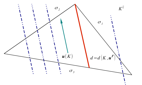
Figure 4: Stream Lines, Volume of Control $K^{\zeta}$, Horizontal View

Figure 4 depicts a fixed volume of control $K^{\zeta}$, the constant velocity $\mathbf{u}(K)$ within and in segmented blue lines the Stream Lines. A simple calculation shows that the Average Length of the Stream Lines is given by $\frac{1}{2}\,d$ where $d=d(K,\mathbf{u}^{\Gamma})$ is the maximum length of the segments parallel to $\mathbf{u}(K)$ contained inside $K^{\zeta}$. Therefore the energy dissipation due to friction is given by

$$\mathcal{F}(\mathbf{u}^{\Gamma})\overset{\textbf{def}}{=}\gamma\;\sum_{K\,\in\,\mathcal{T}}\frac{1}{2}\,|K^{\zeta}|\,d\left(K,\mathbf{u}^{\Gamma}\right)|\mathbf{u}(K)|=\frac{1}{2}\,\gamma\;|\mathbf{u}^{\Gamma}|\sum_{K\,\in\,\mathcal{T}}d\left(K,\mathbf{u}^{\Gamma}\right)|K^{\zeta}|.$$ (37)

In the expression above $\gamma$ is the friction coefficient depending on the material of the walls of the fissure, $|K^{\zeta}|$ is the area of the volume of control $K^{\zeta}$ and $|\mathbf{u}^{\Gamma}|$ is the magnitude of the master velocity $\mathbf{u}^{\Gamma}$. The second equality in (37) uses the fact that, by construction $|\mathbf{u}(K)|=|\mathbf{u}^{\Gamma}|$ for all $K\in\mathcal{T}$. The expression (37) implies that we need to address the question

$$\mathbf{v}^{\Gamma}\in S^{\,1}:\mathcal{F}(\mathbf{v}^{\Gamma})=\min\left\{\mathcal{F}(\mathbf{b}):\mathbf{b}\in S^{\,1}\right\}.$$ (38)

However, the functional $\mathcal{F}\left(\cdot\right)$ does not have the same quadratic structure as $U_{curv}$ or $U_{grav}$ due to the presence of the map $\mathbf{u}^{\Gamma}\mapsto d(K,\mathbf{u}^{\Gamma})$. Although proving the existence of minima is easy to show, characterizing them is extremely difficult. Nevertheless it will be shown that the set of preferential directions can be turned into a suitable probability space. To that end, the function $\mathbf{u}^{\Gamma}\mapsto d(K,\mathbf{u}^{\Gamma})$ needs to be further studied.

4.2 The Minimizing Set of $\mathcal{F}$

We start analyzing a problem closely related to the map $\mathbf{u}^{\Gamma}\mapsto d(K,\mathbf{u}^{\Gamma})$, introducing an auxiliary function

Definition 4.1.

The parametrized inner-segment length function $\chi:\bm{\mathbbm{R}}\rightarrow[0,\infty)$ is defined by

$$\chi(t)\overset{\textbf{def}}{=}d(\cos t,\sin t).$$

It is immediate to see that $\chi$ is $\pi$-periodic. Now consider the following family of particular triangles in $\bm{\mathbbm{R}}^{2}$, see figure 5.

$$\mathcal{C}\overset{\textbf{def}}{=}\{\Delta\subseteq\bm{\mathbbm{R}}^{\!2}:\Delta\;\,\text{is a triangle with one of its sides defined by the unitary vector}\;\,\bm{\widehat{\imath}}\\ \text{ and a second side defined by a vector}\;c\,(\cos\theta,\sin\theta)\text{ for }0<\theta<\pi,\,c>0\}.$$ (39)

With the definition above we have the following result

Proposition 4.2.

Let $\Delta$ be an element of $\mathcal{C}$

1. The parametrized inner-segment length function $\chi:[0,\pi]\rightarrow\bm{\mathbbm{R}}$ is described by the following expression

   $$\chi(t)=\frac{c\,\sin\theta}{c\,\sin(\theta-t)+\sin t}\,\bm{\mathbbm{1}}_{[0,\theta]}+c\,\frac{\sin\theta}{\sin t}\,\bm{\mathbbm{1}}_{[\theta,\,t_{0}]}+\frac{\sin\theta}{\sin(t-\theta)}\bm{\mathbbm{1}}_{[t_{0},\,\pi]}.$$ (40)

   Where $t_{0}\in[0,\pi]$ is such that $(\cos t_{0},\sin t_{0})$ is parallel to the third side $(c\,\cos\theta-1,c\,\sin\theta)$.

2. The function $\chi$ is continuous.

Proof 4.3.

(i) By direct calculation. (ii) Follows directly from the expression (40) in the previous part.

Remark 4.4.

Observe that any triangle in $\Delta\subseteq\bm{\mathbbm{R}}^{2}$ can be reduced to an element of $\mathcal{C}$ by dilation and rotation maps. The first map only amplifies the values of $\chi$, while the second map only shifts the sub-intervals of definition, which will become at most four. In all the cases the function $\chi$ is described by rational trigonometric functions bounded away from singularities.

In order to extend the analysis to the elements of the triangulation we define a new family

$$\mathcal{D}\overset{\textbf{def}}{=}\{\Delta\subseteq\bm{\mathbbm{R}}^{\!3}:\Delta\;\,\text{is a triangle whose orthogonal projection onto the horizontal plane}\,\;\langle\bm{\widehat{k}}\rangle^{\perp},\\ \text{is an element of}\;\,\mathcal{A}\}.$$ (41)

Now we describe the function $\chi$ on the family $\mathcal{D}$.

Proposition 4.5.

Let $\Delta$ be an element of $\mathcal{D}$, $\bm{\widehat{n}}$ be the normal vector orthogonal to $\Delta$ and let $\Delta_{0}$ be the orthogonal projection of $\Delta$ onto the horizontal plane $\langle\bm{\widehat{k}}\rangle^{\perp}$.

1. Let $\chi,\chi_{0}:[0,\pi]\rightarrow\bm{\mathbbm{R}}$ be the respective parametrized inner-segment length functions then, the following relation holds

   $$\chi(t)=\frac{1}{\sqrt{1-(\bm{\widehat{n}}\cdot(\cos t,\sin t,0))^{2}}}\,\chi_{0}(t).$$ (42)

2. The function $\chi:[0,\pi]\rightarrow[0,\infty)$ is continuous.

Proof 4.6.

1. It suffices to observe that the factor affecting $\chi_{0}(t)$ in (42) is the amplification factor on the segment length (or vector norm) due to the “lifting” of the segment $\chi_{0}(t)(\cos t,\sin t)$ contained in $\Delta_{0}$ onto the triangle $\Delta$.

2. Follows immediately from the continuity of $\chi_{0}$ shown in part (ii) of proposition 4.2 and the relation (42) given by the previous part.

Remark 4.7.

Observe that any triangle in $\Delta\subseteq\bm{\mathbbm{R}}^{3}$ can be reduced to an element of $\mathcal{B}$. Denote $\Delta_{0}$ the orthogonal projection of $\Delta$ on the horizontal plane $\langle\bm{\widehat{k}}\rangle^{\perp}$. Then, the dilation and rotation maps that turn $\Delta_{0}$ into an element of $\mathcal{C}$ also turn $\Delta$ into an element of $\mathcal{D}$.

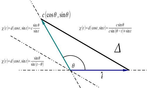
Figure 5: Triangle $\&$ Inner Segments

Theorem 4.8.

Let $\Gamma$ be a piecewise $C^{1}$ surface and $\Gamma_{\scriptscriptstyle\mathcal{H},\mathcal{T}}$ be a triangulation. Then, the functional $\mathcal{F}$ attains its minimum on $S^{1}$.

Proof 4.9.

Using the definition of $\mathcal{F}$, consider the function $X:[0,\pi]\rightarrow[0,\infty)$

$$X(t)\overset{\textbf{def}}{=}\mathcal{F}(\cos t,\sin t)=\frac{1}{2}\,\gamma\sum_{K\,\in\,\mathcal{T}}d\left(K,(\cos t,\sin t)\right)|K^{\zeta}|.$$

Since $X$ is the sum of continuous functions as seen in proposition 4.5 part (ii), the function $X$ is continuous. Since it is defined on the compact set $[0,\pi]$ it must attain its minimum at a point, namely $t_{0}$. Finally, since

$$X(t_{0})=\min\{X(t):t\in[0,\pi]\}\equiv\min\{\mathcal{F}(\mathbf{u}^{\Gamma}):\mathbf{u}^{\Gamma}\in S^{1}\}=\mathcal{F}(\cos t_{0},\sin t_{0}),$$

the result follows.

Lemma 4.10.

Let $\Delta\subseteq\bm{\mathbbm{R}}^{\!3}$ be a triangle, $\chi:[0,\,\pi]\rightarrow[0,\infty)$ its parametrized inner-segment length function and $\{I_{n}:1\leq n\leq N\}$ the disjoint open sub-intervals of piecewise definition, with $N\in\{3,4\}$. Then for each $I_{n}$ the function $\chi|_{I_{n}}$ has an analytic extension to an open connected set $U_{n}$ of the complex plane, containing the closure of $I_{n}$.

Proof 4.11.

Due to propositions 4.2 and 4.5 as well as remarks 4.4, 4.7 we observe that the function $\chi|_{I_{n}}$ is a rational trigonometric function bounded away from singularities. Therefore, the map $z\mapsto\chi(z)$ is well-defined and analytic in a neighborhood of the closure of $I_{n}$ for each $1\leq n\leq N$.

Finally we present the result that will allow us to define the uniform probability on the set of preferential directions.

Theorem 4.12.

Let $\Gamma$ be a piecewise $C^{1}$ surface and $\Gamma_{\scriptscriptstyle\mathcal{H},\mathcal{T}}$ be a triangulation. Then, the minimization set

$$\omega_{friction}\overset{\textbf{def}}{=}\left\{\mathbf{u}^{\Gamma}\in S^{1}:\mathcal{F}(\mathbf{u}^{\Gamma})=\min\left\{\mathcal{F}(\mathbf{v}^{\Gamma}):\mathbf{v}^{\Gamma}\in S^{1}\right\}\right\},$$ (43)

has either a finite number or elements or, it has positive Lebesgue measure.

Proof 4.13.

Let $K$ be an element of $\Gamma_{\mathcal{H},\mathcal{T}}$ and $\chi^{K}:[0,2\,\pi]\rightarrow[0,\infty)$ be its parametrized inner-segment length function, extended by periodicity from $[0,\pi]$ to $[0,2\pi]$. Let $\{t_{j}^{K}:1\leq j\leq J(K)\}$ be the points in $(0,2\,\pi)$ connecting the disjoint sub-intervals $\{I_{n}^{K}:1\leq n\leq N(K)\}$ of definition for $\chi_{K}$; with $J(K)=N(K)-1$ and $N(K)\in\{5,6\}$. Define the set

$$D\overset{\textbf{def}}{=}\{0,\,1\}\bigcup_{K\in\mathcal{T}}\{t_{j}^{K}:1\leq j\leq J(K)\}.$$

This set is finite and therefore it can be ordered monotonically $0=t_{0}<t_{1}<\ldots<t_{J}=2\pi$. Denote $I_{n}\overset{\textbf{def}}{=}(t_{j-1},t_{j})$ for all $1\leq j\leq J$. Let $\{U^{K}_{n}:1\leq n\leq N(K)\}$ be the open sets of analytic extension for $\left.\chi^{K}\right|_{I_{n}}$ such that $cl(I^{K}_{n})\subseteq U^{K}_{n}$. Define the following sets

$$U_{j}\overset{\textbf{def}}{=}\bigcap\{U^{K}_{n}:I_{j}\subseteq I^{K}_{n},\,K\in\mathcal{T}\}\,,\quad 1\leq j\leq J.$$ (44)

The set $U_{j}$ is open connected since it is the finite intersection of open connected sets and since $cl(I_{j})\subseteq cl(I^{K}_{n})\subseteq U^{K}_{n}$ for all the chosen open sets in (44), this implies that $cl(I_{j})\subseteq U_{j}$. Also observe that $\{U_{j}:1\leq j\leq J\}$ is an open covering of the interval $[0,2\,\pi]$. Consider the function $X_{j}:U_{j}\rightarrow\bm{\mathbbm{C}}$

$$X_{j}(z)\overset{\textbf{def}}{=}\frac{1}{2}\,\gamma\sum_{K\,\in\,\mathcal{T}}\left.\chi^{K}\right|_{U_{j}}(z)\;|K^{\zeta}|-\min\{\mathcal{F}(\mathbf{u}^{\Gamma}):\mathbf{u}^{\Gamma}\in S^{1}\}\,,\quad 1\leq j\leq J.$$

This function is also analytic because the map $\left.\chi^{K}\right|_{U_{j}}$ is analytic for all $1\leq j\leq J$. If the minimization set $\omega_{friction}$ defined in (43) contains a finite number of points there is nothing to prove. If it contains infinitely many points, then it has a convergent subsequence to a point $\xi\in[0,2\,\pi]$. Let $U_{j_{0}}$ be one of the sets in the covering $\{U_{j}:1\leq j\leq J\}$ such that $\xi\in U_{j_{0}}$ then, the zeros of the function $X_{j_{0}}$ have a limit point, therefore it must be constant and $\omega_{friction}\supseteq I_{j_{0}}$. Recall that $\omega_{friction}=\mathcal{F}^{-1}(\{\min_{S^{1}}\mathcal{F}\})$ is the inverse image of a point through a continuous function and therefore it is a measurable set. Seeing that the interval $I_{j_{0}}$ is non-degenerate, we conclude that $\omega_{friction}$ has positive Lebesgue measure.

4.3 Probability Space of Preferential Fluid Flow Directions due to Friction

We follow the same reasoning presented in section 2.5. The Preferential Fluid Flow Directions of the surface $\Gamma_{\mathcal{H},\,\mathcal{T}}$ due to Friction are given by

$$\varpi_{friction}\overset{\textbf{def}}{=}\left\{\frac{m(V_{\Gamma_{\mathcal{H},\,\mathcal{T}}}\mathbf{b})}{|m(V_{\Gamma_{\mathcal{H},\,\mathcal{T}}}\mathbf{b})|}:\mathbf{b}\in\omega_{friction}\right\}.$$ (45)

Now we define the natural $\sigma$-algebra on $\varpi_{friction}$.

Definition 4.14.

Let $\Gamma$ be a piecewise $C^{1}$ surface, $\Gamma_{\scriptscriptstyle\mathcal{H},\mathcal{T}}$ be a triangulation and the minimizing set $\omega_{friction}$ defined in (43). Consider the surjective function

$$\varphi:\omega_{friction}\rightarrow\varpi_{curv}\,,\quad\varphi(\bm{\widehat{e}})\overset{\textbf{def}}{=}\frac{m(V_{\Gamma_{\mathcal{H},\,\mathcal{T}}}\bm{\widehat{e}})}{|m(V_{\Gamma_{\mathcal{H},\,\mathcal{T}}}\bm{\widehat{e}})|}.$$ (46)

Let $\beta$ be the Borel tribe in $S^{1}$ intersected with $\omega_{friction}$, define the following $\sigma$-algebra

$$\tau_{friction}\overset{\textbf{def}}{=}\left\{A\in\wp(\varpi_{friction}):\varphi^{-1}(A)\in\beta\right\}.$$ (47)

Where $\wp(\varpi_{friction})$ is the power set of $\varpi_{friction}$.

Finally, we endow the preferential flow space with the uniform probability distribution

Definition 4.15.

Let $\Gamma$ be a piecewise $C^{1}$ surface, $\Gamma_{\scriptscriptstyle\mathcal{H},\mathcal{T}}$ be a triangulation and $\varpi_{friction}$ be the associated preferential fluid flow directions defined in (45) then

1. If $\varpi_{friction}$ is finite, define

   (48)

2. If $\varpi_{friction}$ is infinite, define

   (49)

   Here $\mu$ indicates the arc-length measure in $S^{1}$.

Remark 4.16.

Due to the theorem 4.12 the probability given in the definition above is well-defined. Hence $(\varpi_{friction},\tau_{friction},$ is a probability space.

5 The Global Space of Preferential Fluid Flow Directions and Closing Remarks

In this section we use the Superposition Principle to assemble the effect of the factors analyzed in the previous sections.

5.1 Global Space of Preferential Fluid Flow Directions

In the following assume that $\tau_{curv}$, $\tau_{grav}$ and $\tau_{friction}$ are the $\sigma$-algebras corresponding to each preferential set $\varpi_{curv}$, $\varpi_{grav}$ and $\varpi_{friction}$. If one of the preferential sets is discrete it is assumed that the associated $\sigma$-algebra is its power set. Now we introduce some definitions.

Definition 5.1.

Let $\Gamma$ be a piecewise $C^{1}$ surface and $\Gamma_{\scriptscriptstyle\mathcal{H},\mathcal{T}}$ be a triangulation. The minimizing space associated to the triangulation $\Gamma_{\mathcal{H},\mathcal{T}}$ is defined by

$$\omega\left(\Gamma_{\mathcal{H},\mathcal{T}}\right)\overset{\textbf{def}}{=}\varpi_{curv}\times\ \varpi_{grav}\times\varpi_{friction}\,,$$ (50a)

endowed with the product $$\sigma$$-algebra

$$\tau_{\omega}\overset{\textbf{def}}{=}\tau_{curv}\otimes\tau_{grav}\otimes\tau_{friction}\,,$$ (50b)

and the product probability measure

(50c)

Definition 5.2.

We define the weights of the preferential directions coming from each effect in the following way

$$p_{\,1}\overset{\textbf{def}}{=}\frac{\min U_{curv}}{\min U_{curv}+\min U_{grav}+\min\,\mathcal{F}}\,,$$ (51a)

$$p_{\,2}\overset{\textbf{def}}{=}\frac{U_{width}+\min U_{grav}}{U_{curv}+\min U_{grav}+\min\,\mathcal{F}}\,,$$ (51b)

$$p_{\,3}\overset{\textbf{def}}{=}\frac{\min\,\mathcal{F}}{\min U_{curv}+\min U_{grav}+\min\,\mathcal{F}}\,.$$ (51c)

Next we define the Space of Preferential Directions

Definition 5.3.

Let $\Gamma$ be a piecewise $C^{1}$ surface, $\Gamma_{\scriptscriptstyle\mathcal{H},\mathcal{T}}$ be a triangulation and consider the function $\Phi:\varpi_{curv}\times\varpi_{grav}\times\varpi_{friction}\rightarrow S^{\,2}\cup\{\bm{0}\}$ defined by

$$\Phi(\mathbf{a}_{\,1},\mathbf{a}_{\,2},\mathbf{a}_{\,3})\overset{\textbf{def}}{=}\begin{cases}\dfrac{p_{\,1}\,\mathbf{a}_{\,1}+p_{\,2}\,\mathbf{a}_{\,2}+p_{\,3}\,\mathbf{a}_{\,3}}{\left|p_{\,1}\,\mathbf{a}_{\,1}+p_{\,2}\,\mathbf{a}_{\,2}+p_{\,3}\,\mathbf{a}_{\,3}\right|}&p_{\,1}\,\mathbf{a}_{\,1}+p_{\,2}\,\mathbf{a}_{\,2}+p_{\,3}\,\mathbf{a}_{\,3}\neq\bm{0},\\[8.0pt] \bm{0}&p_{\,1}\,\mathbf{a}_{\,1}+p_{\,2}\,\mathbf{a}_{\,2}+p_{\,3}\,\mathbf{a}_{\,3}=\bm{0}.\end{cases}$$ (52)

The Space of Preferential Directions is given by

$$\varpi\left(\Gamma_{\mathcal{H},\mathcal{T}}\right)\overset{\textbf{def}}{=}\Phi\left(\omega\left(\Gamma_{\mathcal{H},\mathcal{T}}\right)\right)=\Phi\left(\varpi_{curv}\times\ \varpi_{grav}\times\varpi_{friction}\right),$$ (53a)

endowed with the $$\sigma$$-algebra

$$\tau\left(\Gamma_{\mathcal{H},\mathcal{T}}\right)\overset{\textbf{def}}{=}\{A\subseteq\varpi\left(\Gamma_{\mathcal{H},\mathcal{T}}\right):\Phi^{-1}(A)\in\tau_{curv}\otimes\tau_{grav}\otimes\tau_{friction}\,,$$ (53b)

and the probability measure

(53c)

Remark 5.4.

Observe that unlike the previous cases of analysis the direction $\bm{0}$ is actually possible. This would mean that the medium is isotropic: it is the unlikely event that the analyzed effects cancel each other, i.e. they “average out”.

5.2 Entropy of the Preferential Fluid Flow Information

Finally, appealing to Shannon’s information theory Shannon we present a definition of the Geometric Entropy of the triangulation $\Gamma_{\mathcal{H},\mathcal{T}}$, as a measure of the amount of uncertainty in the phenomenon of preferential fluid flow.

Definition 5.5.

Denote $\Sigma\left(\Gamma_{\mathcal{H},\mathcal{T}}\right)$ the family of all countable partitions of $\varpi\left(\Gamma_{\mathcal{H},\mathcal{T}}\right)$ such that each set is $\tau\left(\Gamma_{\mathcal{H},\mathcal{T}}\right)$-measurable.

The concept of entropy on the elements of $\Sigma\left(\Gamma_{\mathcal{H},\mathcal{T}}\right)$ follows naturally Shannon ; Khinchin .

Definition 5.6.

Let $\Gamma$ be a piecewise $C^{1}$ surface, $\Gamma_{\scriptscriptstyle\mathcal{H},\mathcal{T}}$ be a triangulation, $\Sigma\left(\Gamma_{\mathcal{H},\mathcal{T}}\right)$ the family of countable measurable partitions of $\varpi\left(\Gamma_{\mathcal{H},\mathcal{T}}\right)$ and $\mathcal{A}\in\Sigma\left(\Gamma_{\mathcal{H},\mathcal{T}}\right)$.

1. The information function associated to $\mathcal{A}$ is given by

   $$I_{\scriptscriptstyle\mathcal{A}}(x)\overset{\textbf{def}}{=}-\sum_{A\,\in\,\mathcal{A}}\log$$ (54)

2. The Geometric Entropy associated to $\mathcal{A}$ is the expectation of $I_{\mathcal{A}}$, i.e.

   $$\mathbbm{H}\left(\mathcal{A}\right)\overset{\textbf{def}}{=}\int_{\varpi\left(\Gamma_{\mathcal{H},\mathcal{T}}\right)}I_{\scriptscriptstyle\mathcal{A}}(x)d$$ (55)

   In the last expression it is understood that $0\cdot\log 0=0$ in consistency with measure theory.

3. The Geometric Entropy of the triangulation $\Gamma_{\mathcal{H},\mathcal{T}}$ is given by

   $$\mathbbm{H}\left(\Gamma_{\mathcal{H},\mathcal{T}}\right)\overset{\textbf{def}}{=}\sup\{\mathbbm{H}(\mathcal{A}):\mathcal{A}\in\Sigma\left(\Gamma_{\mathcal{H},\mathcal{T}}\right)\}\\ =-\int_{\varpi\left(\Gamma_{\mathcal{H},\mathcal{T}}\right)}p(x)\,\log p(x)\,dx$$ (56)

   Where the last equality holds whenever $d$ has density $p$ with respect to the Lebesgue measure $dx$ in $S^{2}\cup\{\bm{0}\}$. In particular for such density to exist it must hold that .

5.3 Closing Remarks and Future Work

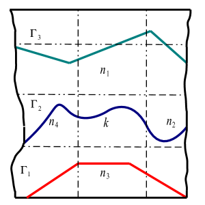
(a) Meshed Fissured Medium

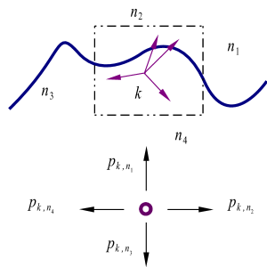
(b) Transmission Probabilities

Figure 6: Meshed Fissured Medium and Transmission Probabilities

Due to analysis exposed, several observations are in order:

1. The method we have presented to determine the probability space of preferential flow directions can be extended to other factors of interest, depending on the framework and available information.

2. The analyzed factors were presented in order of difficulty, not from the mathematical point of view, but from the applicability of its conclusions. Since the curvature effect is reduced to an eigenvalue-eigenvector problem this is the easiest of all. Gravity demands the inclusion of an extra criterion expensive to implement numerically, however, the minimizing set $\omega_{grav}$ is still easy to characterize by an eigenvalue-eigenvector problem. Finally, the friction effect analysis yields results of mere existence, there are no characterizations or constructive clues to find the minimizing set $\omega_{friction}$.

3. The difficulties presented in the analysis by friction come mostly from the non-quadratic structure of the energy dissipation functional $\mathcal{F}$ defined in (37); this makes it highly impractical for applications. In general, whichever considered factor other than the ones presented here, leading to an energy functional whose minimizing set can not be characterized (unlike quadratic or strictly convex functionals) is likely to be impractical for computational purposes.

4. In the aforementioned cases, proving the existence of the associated preferential fluid directions space plays the role of theoretical support for the modeling. However, it may be wiser to use experimental sources of information and incorporate them in the global scheme with the procedure presented in section 5.1 for computational applications.

So far the analysis has been made for a porous medium with one single crack embedded. However, in the future these will be applied to a fissured system, defining a Markov Chain in the following way:

1. Define a grid on the system so that each portion contains at most one crack; see figure 6 (a).

2. On each element the space of preferential fluid flow directions can be defined using the procedure of this work.

3. Let $N$ be the number of elements in the grid. For each element, namely $k$, we define its transmission probabilities $\{p_{k,n}:1\leq k\leq N\}$ as follows. We set $0$ as probability transmission between two elements which do not share a common face. For each face of contact (4 faces on 2-D and 6 faces on 3-D, at most) the transmission probability from the element $k$ to its neighbor is given by the probability that the common face has to be hit by the stream line of a preferential flow direction, starting from the centroid of the element $k$; see 6 (b).

4. Since the transmission probabilities add up to one and they are all non-negative for each element, the procedure described above clearly defines a stochastic matrix. The matrix has null entries on the diagonal. It is also sparse because it has at most 4 non-null entries in 2-D and at most 6 non-null entries in 3-D.

References

- (1) Arbogast, T. & Brunson, D. (2007) A computational method for approximating a Darcy-Stokes system governing a vuggy porous medium. Computational Geosciences, 11, No 3, 207–218.
- (2) Arbogast, T., Douglas, Jr, J. & Hornung, U. (1990) Derivation of the double porosity model of single-phase flow via homogenization theory. SIAM Journal of Mathematical Analysis, 21, 823–836.
- (3) Arbogast, T. & Lehr, H. (2006) Homogenization of a Darcy-Stokes System Modeling Vuggy Porous Media. Computational Geosciences, 10, No 3, 291–302.
- (4) Barenblatt, G., Zheltov, I. & Kochina, I. (1960) Basic concepts in the theory of seepage and homogeneous liquids in fissured rocks. Journal of Applied Mechanics, 24, 1286–1303.
- (5) Batchelor, G. (2002) An Introduction to Fluid Dynamics, Cambridge Mathematical Library. Cambridge University Press, New York.
- (6) Beryland, L. & Golden, K. (1994) Exact results for the effective conductivity of a continuum percolation model. Phys. Rev. B., 50, 2114–2117.
- (7) Bradji, A. & Herbin, R. (2006) On the discretization of the coupled heat and electrical diffusion problems.. Numerical Methods and Applications: 6th International Conference, NMA 2006, Borovets, Bulgaria, Revised Papers. Springer, pp. 1–15.
- (8) Coffield, Jr, D. J. & Spagnuolo, A. M. (2003) Analysis of a multiple-porosity model for a single-phase flow through naturally fractured porous media. Journal of Applied Mathematics, 2003:7, 327–364. dx.doi.org/10.1155/S1110757X03205143.
- (9) Fiori, A. & Jankovic, I. (2012) On preferential flow, channeling and connectivity in heterogeneous poros formations. Mathematical Geosciences, 44, No 2, 133–145. dx.doi.org/10.1007/s11004–011–9365–2.
- (10) Gallouët, T. & Herbin, R. (2000) Finite Volume Methods, vol. 7 of Handbook of Numerical Analysis. P.G. Ciarlet and J.L. Lions (eds.). North-Holland; 1 edition, Amsterdam, The Netherlands.
- (11) Golden, K. (1994) Scaing law for conduction in partially connected systems. Physica A, 207, 213–218.
- (12) Hagerdorn, F., Mohn, J., Schleppi, P. & Flühler, H. (1998) The Role of Rapid Flow Paths for Nitrogen Transformation in a Forest Soil A Field Study with Micro Suction Cups. Soil Science Society of America Journal, 63 (6), 1915–1923. dx.doi.org/10.2136/sssaj1999.6361915x.
- (13) Jacob, B. (1988) Dynamics of Fluids in Porous Media. Dover Publications Inc., New York.
- (14) Jensen, M. B., Hansen, H. C. B. & Magid, J. (2002) Phosphate Sorption to Macropore Wall Materials and Bulk Soil. Water, Air, and Soil Pollution, 137: 1–4, 141–148. dx.doi.org/10.1023/A:1015589011729.
- (15) Khinchin, A. I. (1957) Mathematical foundations of Information Theory, Dover Books on Mathematics. Dover Publications, New York.
- (16) Lesinigo, M., D’Angelo, C. & Quarteroni, A. (2011) A multiscale Darcy-Brinkman model for fluid flow in fractured media. Numerische Mathematik, 117, 717–752. dx.doi.org/10.1007/s00211–010–0343–2.
- (17) McLaren, R., Forsyth, P., Sudicky, E., VanderKwaak, J., Schwarts, F. & Kessler, J. (2000) Flow and transport in fractured tuff at Yucca Mountain: numerical experiments on fast preferential flow mechanisms. Journal of Contaminant Hydrology, 43(3-4), 211–238. dx.doi.org/10.1016/S0169–7722(00)00085–1.
- (18) Morales, F. A. (2013) On the homogenization of geological fissured systems with curved nonn-periodic cracks. arXiv:1312.4033v1.
- (19) Morales, F. A. & Showalter, R. (2012) Interface Approximation of Darcy Flow in a Narrow Channel. Mathematical Methods in the Applied Sciences, 35, 182–195.
- (20) Sears, F. W. & Salinger, G. L. (1975) Thermodynamics, Kinetic Theory, and Statistical Thermodynamics (3rd Edition), Principles of Physics Series. Addison-Wesley Publishing Company, Inc., Reading, Massachusetts, USA.
- (21) Shannon, C. E. (1971) The mathematical theory of communication. University of Illinois Press; First Edition, Il.
- (22) Showalter, R. (1997) Microstructure Models of Porous Media. In Ulrich Hornung editor Homogenization and Porous Media, vol. 6 of Interdisciplinary Applied Mathematics. Springer-Verlag, New York.
- (23) Showalter, R. E. & Walkington, N. J. (1991) Micro-structure models of diffusion in fissured media. Journal of Mathematical Analysis and Applications, 155, 1–20.
- (24) Spagnuolo, A. M. & Wright, S. (2003) Analysis of a multiple-porosity model for a single-phase flow through naturally fractured porous media. Journal of Applied Mathematics, 2003:7, 327–364. dx.doi.org/10.1155/S1110757X03205143.
- (25) Visarraga, D. & Showalter, R. (2004) Double-diffusion models from a highly-heterogeneous medium. Jour. Math. Anal. Appl, 295(4), 191–210.
- (26) Wang, S., Feng, Q. & Han, X. (2013) A Hybrid Analytical/Numerical Model for the Characterization of Preferential Flow Path with Non-Darcy Flow. PLoS ONE, 8(12), e83536. doi:10.1371/journal.pone.0083536.